A robust optimization approach to synchromodal container transportation I. Chiscop Graduation thesis MSc Applied Mathematics

Welcome message from author
This document is posted to help you gain knowledge. Please leave a comment to let me know what you think about it! Share it to your friends and learn new things together.
Transcript

A robust optimization approachto synchromodal containertransportation
I. Chiscop
Graduation thesisMSc Applied Mathematics

A robust optimization approachto synchromodal container
transportationby
I. Chiscop
to obtain the degree of Master of Scienceat the Delft University of Technology,
to be defended publicly on Friday August 31, 2018 at 10:00 AM.
Student number: 4540107Project duration: January 5, 2018 – August 25, 2018Thesis committee: Prof. dr. E. de Klerk, TU Delft, supervisor
Dr. ir. G. F. Nane, TU DelftDr. F. Phillipson, TNOIr. A. Sangers, TNO
An electronic version of this thesis is available at http://repository.tudelft.nl/.


AbstractThis thesis addresses synchromodal planning at operational level from the perspective of a logisticsservice provider. The existing infrastructure and the transportation activities are studied and modeledas an optimization problem with simultaneous vehicle routing and container-to-mode assignment. Aspecial characteristic of this problem is the uncertain data. In other words, it is assumed that the re-lease times of the containers belong to an uncertainty interval, and no further statistical information isavailable. The problem is then classified according to an extensive framework previously developedwithin the project. An extensive body of literature is reviewed to identify current modeling approachesand their theoretical and practical limitations. This literature study shows that, although discrete timemodels have been intensively investigated, there are few studies which propose continuous model-ing of time. The container routing problem is modeled as a mixed integer program with explicit timevariables and lateness penalties. A robust formulation is then proposed to eliminate the uncertain pa-rameters from the objective function and constraints. By solving the new model exactly, with the aidof an optimization solver, robust solutions are obtained corresponding to transportation plans whichremain feasible for any realization of the release times within the pre-specified uncertainty interval. Inorder to introduce some flexibility in the transportation plan, the continuous time variables are modeledas affine functions of the uncertain parameters. The resulting two-stage decision model is tested for asmall-sized instance in both situations, with high and low lateness penalties. The computational resultsshow that the adjustable robust model yields on the one hand, route-dependent adjusted solutions forthe case of penalized lateness, and on the other hand, a direct improvement of the objective function forthe case of tolerated lateness. The results suggest that the adjustable robust optimization frameworkhas sufficient potential to model the synchromodal container routing problem. This thesis concludeswith addressing some of the limitations of the proposed model and indicating concrete approaches forcountering them.
iii


PrefaceThis thesis report is the final step towards obtaining my master’s degree at Delft University of Technol-ogy. Carrying out this project has been an interesting and eventful journey, and I would like to addressa few words of thanks to those who have helped me along the way.
First of all I would like to express my gratitude to my supervisors Etienne de Klerk (TU Delft), FrankPhillipson (TNO) and Alex Sangers (TNO) for providing the guidance, interest and knowledge that wereso needed in my project, and for allowing me to pursue my ideas freely. Moreover, I would like to thankTina Nane for her willingness to be part of my thesis committee.
Special thanks go to the entire Cybersecurity and Robustness department at TNO for providing a greatwork environment. I would like to thank Kishan and Lianne, my closest collaborators in the project, andthe rest of the interns for the very happy and friendly atmosphere.
Now that my studies have come to an end, I realize that moving to Delft was probably one of thebest decisions I ever made. Besides getting a good education, I had the chance of meeting so manyspecial people to whom I greatly owe my happiness. I am grateful to my best friend Elena for the con-tinuous support, to Piotr, Dennis, and the guys, for kindly adopting me in their group, to Beatrice andBlane, for the laughs and the home-cooked dinners. I have also been most fortunate to cross pathswith Tom, to whom I would like to thank for all the love and encouragement.
Finally, my outmost gratitude goes to my parents and little brother, who have managed to supportme in every way, despite the few thousands kilometers between us. This thesis is dedicated to them.
I. ChiscopDelft, August 2018
v

Contents
1 Introduction 11.1 Synchromodality context . . . . . . . . . . . . . . . . . . . . . . . . . . . . . . . . . . . . 11.2 Problem description . . . . . . . . . . . . . . . . . . . . . . . . . . . . . . . . . . . . . . 2
1.2.1 Practical setting. . . . . . . . . . . . . . . . . . . . . . . . . . . . . . . . . . . . . 31.2.2 Base instance. . . . . . . . . . . . . . . . . . . . . . . . . . . . . . . . . . . . . . 5
1.3 Research question . . . . . . . . . . . . . . . . . . . . . . . . . . . . . . . . . . . . . . . 71.4 Report structure . . . . . . . . . . . . . . . . . . . . . . . . . . . . . . . . . . . . . . . . 7
2 Literature review 92.1 A look towards synchromodality . . . . . . . . . . . . . . . . . . . . . . . . . . . . . . . . 92.2 Intermodal transportation. . . . . . . . . . . . . . . . . . . . . . . . . . . . . . . . . . . . 11
2.2.1 Strategic planning problems . . . . . . . . . . . . . . . . . . . . . . . . . . . . . . 112.2.2 Tactical planning problems . . . . . . . . . . . . . . . . . . . . . . . . . . . . . . . 122.2.3 Operational planning problems . . . . . . . . . . . . . . . . . . . . . . . . . . . . 12
2.3 Contribution made by this work . . . . . . . . . . . . . . . . . . . . . . . . . . . . . . . . 14
3 Overview of existing models 153.1 Discrete-time multicommodity flow problems . . . . . . . . . . . . . . . . . . . . . . . . . 15
3.1.1 The minimum cost multicommodity flow problem on a space-time network . . . . . 153.1.2 The minimum cost multicommodity flow problem with stochastic elements . . . . . 18
3.2 Multicommodity flow problems with continuous time variables . . . . . . . . . . . . . . . . 203.2.1 Multicommodity scheduled service network design. . . . . . . . . . . . . . . . . . 203.2.2 Multicommodity bulk shipping . . . . . . . . . . . . . . . . . . . . . . . . . . . . . 24
4 Deterministic problem formulation 274.1 Deterministic model . . . . . . . . . . . . . . . . . . . . . . . . . . . . . . . . . . . . . . 274.2 Additional remarks . . . . . . . . . . . . . . . . . . . . . . . . . . . . . . . . . . . . . . . 30
5 Robust problem formulation 315.1 Robust optimization paradigm . . . . . . . . . . . . . . . . . . . . . . . . . . . . . . . . . 31
5.1.1 The robust counterpart . . . . . . . . . . . . . . . . . . . . . . . . . . . . . . . . . 325.1.2 Adjustable robust optimization . . . . . . . . . . . . . . . . . . . . . . . . . . . . . 335.1.3 Robust optimization for mixed integer programs . . . . . . . . . . . . . . . . . . . 34
5.2 Robust model . . . . . . . . . . . . . . . . . . . . . . . . . . . . . . . . . . . . . . . . . . 35
6 Computational results 396.1 Instance generation . . . . . . . . . . . . . . . . . . . . . . . . . . . . . . . . . . . . . . 396.2 Results of deterministic model . . . . . . . . . . . . . . . . . . . . . . . . . . . . . . . . . 406.3 Results of robust model . . . . . . . . . . . . . . . . . . . . . . . . . . . . . . . . . . . . 41
6.3.1 High lateness penalties . . . . . . . . . . . . . . . . . . . . . . . . . . . . . . . . 416.3.2 Low lateness penalties . . . . . . . . . . . . . . . . . . . . . . . . . . . . . . . . . 43
6.4 Discussion . . . . . . . . . . . . . . . . . . . . . . . . . . . . . . . . . . . . . . . . . . . 44
7 Conclusion 477.1 Conclusions. . . . . . . . . . . . . . . . . . . . . . . . . . . . . . . . . . . . . . . . . . . 477.2 Recommendations . . . . . . . . . . . . . . . . . . . . . . . . . . . . . . . . . . . . . . . 48
A Distance matrix and cost derivation for base instance 49
Bibliography 51
vii

1Introduction
1.1. Synchromodality contextFreight transportation plays an essential role in supply chains by providing the efficient movement offeedstock, goods and finished products between producers and consumers. In the European Union(EU) particularly, freight transport accounts for almost 4.5% of the gross domestic product (GDP), whilstthe shipping carries 90% of the EU’s foreign trade [10]. However, freight transport also raises a num-ber of issues such as pollutant emissions, noise and congestion, which are mainly due to the roadtransport. A few figures illustrate this assertion. In 2014 about 49% of the total freight transportationin EU countries was done via road, 11.7% via rail, 4.3% via inland waterways and 31.8% by sea1 [29].In terms of pollution, 72.9% of Greenhouse gas (GHG) emissions are due to road transport, 12.8% tomaritime and 0.5% due to railways [2]. To address both the issues of congestion and polluting emis-sions, a modal shift has become desirable [48]. In order to explain this concept, we will briefly reviewthe existing transport modes.
Nowadays freight transport is mostly carried out using containers of standardized dimensions. Thesecan be loaded and unloaded, stacked, transported efficiently over long distances, and transferred fromone mode of transport to another (container ships, rail transport flatcars, and semi-trailer trucks) with-out being opened. The handling system is completely mechanized such that all handling is done withcranes and special forklift trucks. All containers have their own identification number and are trackedusing computerized systems. These aspects make containers a preferable choice for goods trans-portation. The transportation chain of such containers is partitioned in three different segments [44]:pre-haul (first mile for the pickup process at the customer’s warehouse for instance), long-haul (transitof containers between different ports) and end-haul (last mile for the delivery process at the distributioncenter). In most cases, the origin or destination of containers is located in the hinterland and thereforethe pre-haul and end-haul transportation is carried out by road. For the long-haul however, multipletransportation modes are available such as road, rail and waterways. In this scenario, we distinguishseveral types of transportation whose terminology is well-established in literature. We distinguish be-tween unimodal transportation (transporting load by means of only one transportation mode) and mul-timodal transportation (using multiple modes). We further elaborate on different types of multimodaltransportation. In intermodal freight transportation a load is transported from origin to destination inone transportation unit without handling the goods themselves when changing modes [44]. The threesegment container transport chain previously described is an example of intermodal transport. Co-modal transportation as defined in [50], is the intelligent use of two or more modes of transport by a(group of) shipper(s) in a distribution system, either on their own or in combination, in order to obtainthe best benefit from each mode, in terms of overall sustainability. Synchromodal freight transportationis the next step in terms of development, based on an efficient combination of intermodal and co-modaltransportation. The Platform Synchromodality provides the following definition: ”Synchromodality isthe optimally flexible and sustainable deployment of different modes of transport in a network under1There is a certain amount of freight transport carried out by cargo aircrafts. However this is not relevant for the scope of thisthesis.
1
2 1. Introduction
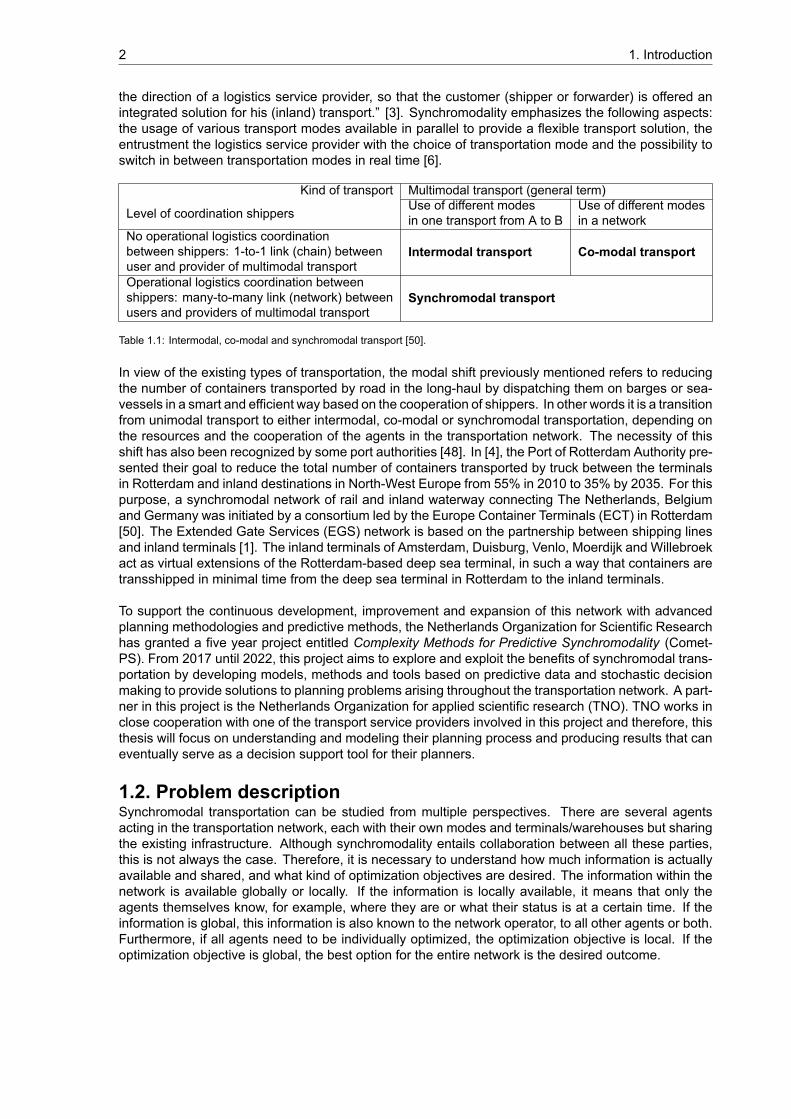
the direction of a logistics service provider, so that the customer (shipper or forwarder) is offered anintegrated solution for his (inland) transport.” [3]. Synchromodality emphasizes the following aspects:the usage of various transport modes available in parallel to provide a flexible transport solution, theentrustment the logistics service provider with the choice of transportation mode and the possibility toswitch in between transportation modes in real time [6].
Kind of transport Multimodal transport (general term)
Level of coordination shippers Use of different modesin one transport from A to B
Use of different modesin a network
No operational logistics coordinationbetween shippers: 1-to-1 link (chain) betweenuser and provider of multimodal transport
Intermodal transport Co-modal transport
Operational logistics coordination betweenshippers: many-to-many link (network) betweenusers and providers of multimodal transport
Synchromodal transport
Table 1.1: Intermodal, co-modal and synchromodal transport [50].
In view of the existing types of transportation, the modal shift previously mentioned refers to reducingthe number of containers transported by road in the long-haul by dispatching them on barges or sea-vessels in a smart and efficient way based on the cooperation of shippers. In other words it is a transitionfrom unimodal transport to either intermodal, co-modal or synchromodal transportation, depending onthe resources and the cooperation of the agents in the transportation network. The necessity of thisshift has also been recognized by some port authorities [48]. In [4], the Port of Rotterdam Authority pre-sented their goal to reduce the total number of containers transported by truck between the terminalsin Rotterdam and inland destinations in North-West Europe from 55% in 2010 to 35% by 2035. For thispurpose, a synchromodal network of rail and inland waterway connecting The Netherlands, Belgiumand Germany was initiated by a consortium led by the Europe Container Terminals (ECT) in Rotterdam[50]. The Extended Gate Services (EGS) network is based on the partnership between shipping linesand inland terminals [1]. The inland terminals of Amsterdam, Duisburg, Venlo, Moerdijk and Willebroekact as virtual extensions of the Rotterdam-based deep sea terminal, in such a way that containers aretransshipped in minimal time from the deep sea terminal in Rotterdam to the inland terminals.
To support the continuous development, improvement and expansion of this network with advancedplanning methodologies and predictive methods, the Netherlands Organization for Scientific Researchhas granted a five year project entitled Complexity Methods for Predictive Synchromodality (Comet-PS). From 2017 until 2022, this project aims to explore and exploit the benefits of synchromodal trans-portation by developing models, methods and tools based on predictive data and stochastic decisionmaking to provide solutions to planning problems arising throughout the transportation network. A part-ner in this project is the Netherlands Organization for applied scientific research (TNO). TNO works inclose cooperation with one of the transport service providers involved in this project and therefore, thisthesis will focus on understanding and modeling their planning process and producing results that caneventually serve as a decision support tool for their planners.
1.2. Problem descriptionSynchromodal transportation can be studied from multiple perspectives. There are several agentsacting in the transportation network, each with their own modes and terminals/warehouses but sharingthe existing infrastructure. Although synchromodality entails collaboration between all these parties,this is not always the case. Therefore, it is necessary to understand how much information is actuallyavailable and shared, and what kind of optimization objectives are desired. The information within thenetwork is available globally or locally. If the information is locally available, it means that only theagents themselves know, for example, where they are or what their status is at a certain time. If theinformation is global, this information is also known to the network operator, to all other agents or both.Furthermore, if all agents need to be individually optimized, the optimization objective is local. If theoptimization objective is global, the best option for the entire network is the desired outcome.
1.2. Problem description 3
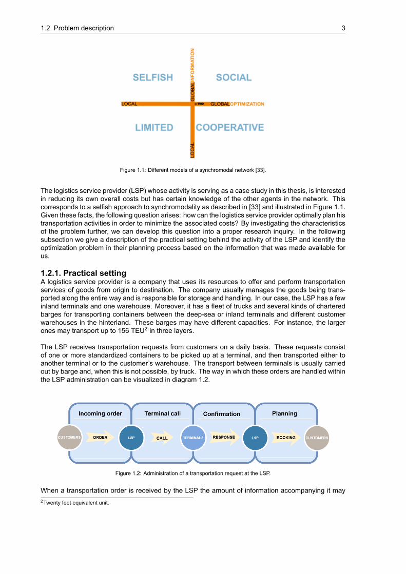
Figure 1.1: Different models of a synchromodal network [33].
The logistics service provider (LSP) whose activity is serving as a case study in this thesis, is interestedin reducing its own overall costs but has certain knowledge of the other agents in the network. Thiscorresponds to a selfish approach to synchromodality as described in [33] and illustrated in Figure 1.1.Given these facts, the following question arises: how can the logistics service provider optimally plan histransportation activities in order to minimize the associated costs? By investigating the characteristicsof the problem further, we can develop this question into a proper research inquiry. In the followingsubsection we give a description of the practical setting behind the activity of the LSP and identify theoptimization problem in their planning process based on the information that was made available forus.
1.2.1. Practical settingA logistics service provider is a company that uses its resources to offer and perform transportationservices of goods from origin to destination. The company usually manages the goods being trans-ported along the entire way and is responsible for storage and handling. In our case, the LSP has a fewinland terminals and one warehouse. Moreover, it has a fleet of trucks and several kinds of charteredbarges for transporting containers between the deep-sea or inland terminals and different customerwarehouses in the hinterland. These barges may have different capacities. For instance, the largerones may transport up to 156 TEU2 in three layers.
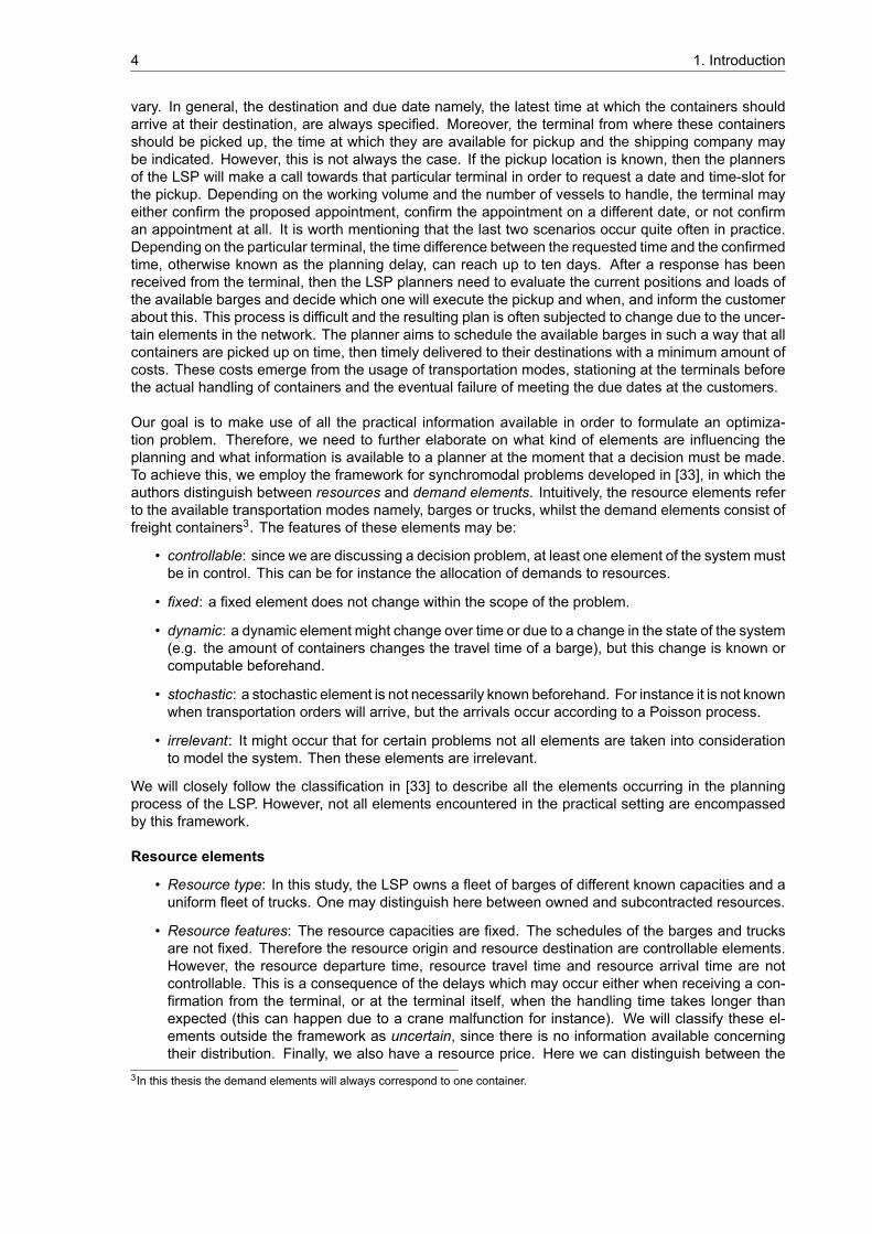
The LSP receives transportation requests from customers on a daily basis. These requests consistof one or more standardized containers to be picked up at a terminal, and then transported either toanother terminal or to the customer’s warehouse. The transport between terminals is usually carriedout by barge and, when this is not possible, by truck. The way in which these orders are handled withinthe LSP administration can be visualized in diagram 1.2.
Figure 1.2: Administration of a transportation request at the LSP.
When a transportation order is received by the LSP the amount of information accompanying it may2Twenty feet equivalent unit.
4 1. Introduction
vary. In general, the destination and due date namely, the latest time at which the containers shouldarrive at their destination, are always specified. Moreover, the terminal from where these containersshould be picked up, the time at which they are available for pickup and the shipping company maybe indicated. However, this is not always the case. If the pickup location is known, then the plannersof the LSP will make a call towards that particular terminal in order to request a date and time-slot forthe pickup. Depending on the working volume and the number of vessels to handle, the terminal mayeither confirm the proposed appointment, confirm the appointment on a different date, or not confirman appointment at all. It is worth mentioning that the last two scenarios occur quite often in practice.Depending on the particular terminal, the time difference between the requested time and the confirmedtime, otherwise known as the planning delay, can reach up to ten days. After a response has beenreceived from the terminal, then the LSP planners need to evaluate the current positions and loads ofthe available barges and decide which one will execute the pickup and when, and inform the customerabout this. This process is difficult and the resulting plan is often subjected to change due to the uncer-tain elements in the network. The planner aims to schedule the available barges in such a way that allcontainers are picked up on time, then timely delivered to their destinations with a minimum amount ofcosts. These costs emerge from the usage of transportation modes, stationing at the terminals beforethe actual handling of containers and the eventual failure of meeting the due dates at the customers.
Our goal is to make use of all the practical information available in order to formulate an optimiza-tion problem. Therefore, we need to further elaborate on what kind of elements are influencing theplanning and what information is available to a planner at the moment that a decision must be made.To achieve this, we employ the framework for synchromodal problems developed in [33], in which theauthors distinguish between resources and demand elements. Intuitively, the resource elements referto the available transportation modes namely, barges or trucks, whilst the demand elements consist offreight containers3. The features of these elements may be:
• controllable: since we are discussing a decision problem, at least one element of the systemmustbe in control. This can be for instance the allocation of demands to resources.
• fixed: a fixed element does not change within the scope of the problem.
• dynamic: a dynamic element might change over time or due to a change in the state of the system(e.g. the amount of containers changes the travel time of a barge), but this change is known orcomputable beforehand.
• stochastic: a stochastic element is not necessarily known beforehand. For instance it is not knownwhen transportation orders will arrive, but the arrivals occur according to a Poisson process.
• irrelevant: It might occur that for certain problems not all elements are taken into considerationto model the system. Then these elements are irrelevant.
We will closely follow the classification in [33] to describe all the elements occurring in the planningprocess of the LSP. However, not all elements encountered in the practical setting are encompassedby this framework.
Resource elements
• Resource type: In this study, the LSP owns a fleet of barges of different known capacities and auniform fleet of trucks. One may distinguish here between owned and subcontracted resources.
• Resource features: The resource capacities are fixed. The schedules of the barges and trucksare not fixed. Therefore the resource origin and resource destination are controllable elements.However, the resource departure time, resource travel time and resource arrival time are notcontrollable. This is a consequence of the delays which may occur either when receiving a con-firmation from the terminal, or at the terminal itself, when the handling time takes longer thanexpected (this can happen due to a crane malfunction for instance). We will classify these el-ements outside the framework as uncertain, since there is no information available concerningtheir distribution. Finally, we also have a resource price. Here we can distinguish between the
3In this thesis the demand elements will always correspond to one container.
1.2. Problem description 5
price for employing a certain resource which is a fixed amount (per day for instance) and the pricefor handling services provided at the terminals. The latter depends on the load to be handled,which is an uncertain element at the beginning of the planning period.
• Terminal Handling time: This refers to time required to handle different types of modes at theterminal. It includes both the waiting time and the time allocated for loading/unloading containers.This is also an uncertain element since there exist incoming orders which do not specify the pickuptime or locations. For instance, it may be the case that a barge is waiting at a terminal to pick upsome containers which have not arrived there yet.
Demand elements
• Demand type: The LSP under study can transport containers of different sizes, of either 1 TEUor 2 TEU in load. Therefore, this element is fixed.
• Demand-to-Resource allocation: The assignment of containers to barges is essentially a decisionthat a planners have to make. Therefore, it is a controlled element.
• Demand features: The destination of a container, as well as its volume (in TEU) and due dateat the customer to whom it belongs, are fixed elements. The demand origin (pick up terminalof a container) and its release date (moment in time at which it can be loaded on a barge) areuncertain elements. This uncertainty emerges from the missing data in the transportation order,as customers simply do not specify it.
• Demand Penalty: This term refers to costs that are incurred when the due date at the destinationfor a container is not met. Since these costs are in general customer-dependent, we can classifythis element as dynamic.
The resource and demand elements described are the main input for creating a schedule for the bargesand trucks. However, the planning process does not only rely on the information that is available, butalso on the moment at which this information becomes available. At the beginning of the planning pe-riod, the planner knows the exact locations of all the barges and trucks in the fleet, their capacity, andhas a list of orders with specified destinations and due dates to be picked up sometime in the next ninedays. Moreover, at every moment in time, a planner has an estimation of the maximum and average de-lay of the deep sea terminals (based on historic data in the last thirty days). This is the initial amount ofknowledge. As time progresses, more information becomes available. That is, pickup locations alongwith release times of containers are revealed, and terminals send confirmation for appointment times.Moreover, new transportation orders may come in, which are also required to be executed within thenext 9 days. This information can become available at any time so the planner must create a schedulethat can handle real-time switches.
Given this practical setting, one may formulate the decision making of the LSP planners as an opti-mization problem in which a routing of transportation modes and an assignment of the containers tomodes must be provided under uncertain data in such a way that the total delay and costs are mini-mized.
1.2.2. Base instanceIn order to be able to develop a mathematical model and later on explore solution methods, we considerthe following simplified instance obtained by reducing the size of the real-life problem and introducingsome assumptions. The network comprises of the following elements:
• 2 customers denoted 𝐶 , 𝐶 : their physical location is known and it is accesible only by truck.
• 2 deep-sea terminals denoted 𝑇 , 𝑇 : deep-sea vessel arrive here and unload the containers thatbelong to the two customers.
• 1 container terminal operated by the LSP denoted 𝑇: barges leave from here and go to the deep-sea terminals to pick up containers.
• 1 hinterland terminal operated by the LSP denoted 𝐷: it is the central terminal of the LSP, closestin distance to any customer.
6 1. Introduction
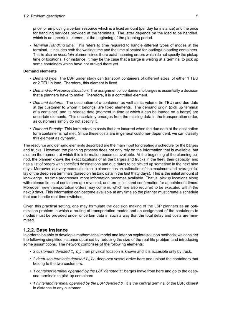
We notice here that there is one main difference between the container terminal and the hinterlandterminal of the LSP. The container terminal is the located in the port, nearby deep-sea terminals. Onthe other hand, the hinterland terminal is situated further away on the continent, in the proximity ofcustomers. This is illustrated in Figure 1.3.
Figure 1.3: Geographical display of the network.
The LSP has the following resources:
• 3 barges: all with capacity of 20 units. Two of the barges at the terminal 𝑇 whilst the other one issituated at the central terminal 𝐷. There is a fixed cost per kilometer4 traveled by a barge.
• unlimited trucks: all with capacity 1. There is a fixed cost per kilometer traveled by a truck.
Suppose we are given two transportation orders with the following specifications:
1. Customer 𝐶 asked the LSP to pickup 30 containers from 𝑇 . The terminal has confirmed a timewindow for the pickup: [10, 11]5. These containers have an uncertain release time. They willbe simultaneously released sometime in the interval [10, 11]. This order needs to arrive at thecustomer by time unit 20.
2. Customer 𝐶 has 10 containers to be picked up from terminal 𝑇 . This terminal has also confirmeda time window for the pickup: [15, 16]. All 10 containers are already available. This order needsto arrive at the customer warehouse by time unit 20.
When developing this base model we have made several assumptions. We discuss them and theirrelation with the real practical setting below.
• The planning period starts at midnight or otherwise interpreted, at time step 0 and covers one fullday, until time step 24 respectively.
• We assume fixed time windows at the deep-sea terminals. In practice we saw that a terminal caneither answer an appointment call or not. In this scenario, we assume that we have confirmedappointment calls at the beginning of the planning period.
• If a barge arrives either too early or too late at a deep-sea terminal, it can be handled right away.So we assume that there is no waiting time involved.
• We assume that there is no handling time.
• Once it has been loaded, a barge may leave the deep-sea terminal right away.
• At any point in time, there are trucks available at every terminal, which can transport the releasedcontainers to other locations.
4We will elaborate on transportation costs of barges and trucks later in the thesis.5We will take a time unit as being one hour. Therefore, regard this interval as the time between 10:00 and 11:00.
1.3. Research question 7
• There is a waterway connecting the terminals. The customers’ warehouses can only be reachedby truck.
• The travel times in between any two locations of the barges and trucks are known.
Given this simple instance, we are interested in minimizing the overall costs and the total delay at thecustomers. In order to maintain a uniform objective, we can associate costs with the delay in such away that the final objective will represents the costs overall. This simple instance will serve as a start-ing point in developing a mathematical model that determines an assignment of containers to transportmodes, and also a specific routing of the containers. Whilst this base model is not of any practical rel-evance, it will serve as a basic tool to understand, and later on, to incorporate more complex featuresof the transport network.
After analyzing the base instance, we understand that our choice for modeling approaches is some-what restricted by the lack of probabilistic knowledge. In this case, we will study the container routingproblem from a robust perspective. In other words, since we cannot employ stochastic models, we willlook at robust optimization techniques.
1.3. Research questionIn view of the instance example introduced in the previous section, we can formulate the following re-search question:How can we simultaneously provide a container-to-mode assignment and a routing of modali-ties under uncertain data and with the objective of minimizing the total costs?We can provide an answer by first tackling these sub-questions:
1. How can we model the simple instance described in Section 1.2.2 in order to encompass all theassumptions?
2. What solution methods can be used to obtain a schedule and container assignment for everymodality?
3. What can be said about the quality and practical relevance of our solution?
4. Does the chosen approach successfully incorporate elements of synchromodality?
1.4. Report structureThis report has been organized in the following way. Chapter 1 gives an introduction into synchromodalcontainer transport and presents a simplified instance of the general problem under study. The relevantliterature concerning synchromodal and intermodal transport planning at different levels is reviewed inChapter 2. Chapter 3 gives an overview of the most common modeling approaches for container trans-port encountered in literature. A deterministic problem formulation is presented in the fourth chapter,followed by the robust approach in Chapter 5. The results of our computational study are summa-rized and discussed in Chapter 6. The final part of this report, namely Chapter 7, is dedicated to theconclusions and some recommendations for related future work.

2Literature review
In this chapter we review some of the existing literature on synchromodal problems in order to presentthe current state of the research progress in this field. As discussed in the previous chapter, synchro-modality is a relatively new concept which aims to enhance the efficiency of intermodal and unimodaltransport networks. Therefore, developing methods for a synchromodal planning relies heavily on ad-vancing and refining the existing approaches to well-studied intermodal and unimodal problems. Due tothis fact, we will include in our summary not only literature which relates to synchromodality directly, butalso papers that tackle freight transportation problems in a more general perspective, without focusingon the real-time switching or cooperation between the agents present in the transportation network.
Synchromodal transportation problems can be classified according to the time span of the decisionswhich must be made. Crainic and Laporte [28] describe three levels of decision problems: strategic(long term), tactical (medium term) and operational (short term) decisions. Strategic planning at acompany level refers to decision taken by the highest level of management, involving a large capitalinvestment over a long period of time. Examples of strategic decisions include the design of the phys-ical network, the location of main facilities (terminals, rail yards etc.) and resource acquisition (fleet ofbarges and trucks). Tactical planning problems refer to the rational and efficient allocation and use ofthe existing resources over a medium term horizon. Tactical decisions concern aspects such as thegeneral operating rules for each terminal, the work allocation among terminals and the choice of routeand service to operate. Finally, operational planning is performed by local management and concernsactivities which are about to take place. The most important operational decisions relate to schedulingthe transport and maintenance services, routing and dispatching of vehicles and allocating resources(freight) to transport modes. These three types of decisions can be visualized in Figure 2.1. We willuse this distinction to further structure our literature survey.
2.1. A look towards synchromodalityTavasszy, Behdani and Konings [47] give a first outlook upon synchromodality. They provide a de-tailed description of the trends in intermodal European transportation from the beginning of container-ized barge transport on the river Rhyne in the 1960’s to present. To keep up with the growing trend offreight demand, the number of barge and rail terminals in ports is increasing. The authors regard thisas the main cause for fragmented container flows and transport inefficiency, as a barge needs to loadfreight at multiple terminals. In this scenario, they highlight the necessity for an integrated view in theplanning and management of different modalities. This refers to the combination of transport serviceson different modalities to provide a customized service to a shipper with a particular type of product totransport and a specific set of logistics requirements. Integrated service planning along with the sub-sequent real-time switching between modalities are the two elements of synchromodality discussed indetail in this paper.
Van Riessen, Negenborn and Dekker [49] provide an overview of relevant topics and research op-portunities in synchromodal container transport. This overview is however limited in the sense that the
9
10 2. Literature review
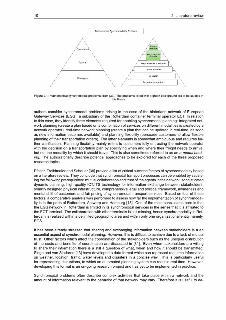
Figure 2.1: Mathematical synchromodal problems, from [33]. The problems listed with a green background are to be studied inthis thesis.
authors consider synchromodal problems arising in the case of the hinterland network of EuropeanGateway Services (EGS), a subsidiary of the Rotterdam container terminal operator ECT. In relationto this case, they identify three elements required for enabling synchromodal planning: integrated net-work planning (create a plan based on a combination of services on different modalities is created by anetwork operator), real-time network planning (create a plan that can be updated in real-time, as soonas new information becomes available) and planning flexibility (persuade customers to allow flexibleplanning of their transportation orders). The latter elements is somewhat ambiguous and requires fur-ther clarification. Planning flexibility mainly refers to customers fully entrusting the network operatorwith the decision on a transportation plan by specifying when and where their freight needs to arrive,but not the modality by which it should travel. This is also sometimes referred to as an a-modal book-ing. The authors briefly describe potential approaches to be explored for each of the three proposedresearch topics.
Pfoser, Treiblmaier and Schauer [38] provide a list of critical success factors of synchromodality basedon a literature review. They conclude that synchromodal transport processes can be enabled by satisfy-ing the following prerequisites: mutual collaboration and trust of the agents in the network, sophisticateddynamic planning, high quality ICT/ITS technology for information exchange between stakeholders,smartly designed physical infrastructure, comprehensive legal and political framework, awareness andmental shift of customers and fair pricing of synchromodal transport services. Based on four of thesefactors, a comparative analysis was performed to assess how far the implementation of synchromodal-ity is in the ports of Rotterdam, Antwerp and Hamburg [18]. One of the main conclusions here is thatthe EGS network in Rotterdam is limited in its synchromodal services in the sense that it is affiliated tothe ECT terminal. The collaboration with other terminals is still missing, hence synchromodality in Rot-terdam is realized within a delimited geographic area and within only one organizational entity namely,EGS.
It has been already stressed that sharing and exchanging information between stakeholders is a anessential aspect of synchromodal planning. However, this is difficult to achieve due to a lack of mutualtrust. Other factors which affect the coordination of the stakeholders such as the unequal distributionof the costs and benefits of coordination are discussed in [31]. Even when stakeholders are willingto share their information there is a still a question of what, when and how it should be transmitted.Singh and van Sinderen [43] have developed a data format which can represent real-time informationon weather, location, traffic, water levels and disasters in a concise way. This is particularly usefulfor representing disruptions, to which an automated planning system can react in real-time. However,developing this format is an on-going research project and has yet to be implemented in practice.
Synchromodal problems often describe complex activities that take place within a network and theamount of information relevant to the behavior of that network may vary. Therefore it is useful to de-
2.2. Intermodal transportation 11
scribe these problems in a comprehensive and consistent way. In [33] a framework is proposed to bothclassify the problems and ease the search for solution methods. We have already made use of thisframework in Chapter 1, to describe the elements in our problem.
This is a brief overview of the most relevant papers in which synchromodality is the main topic. Amore extended literature review, also including a categorization of papers according to pre-requisites,activities and effects of synchromodality can be found in [42]. For a more general literature review onmultimodal freight transport planning, concerning both planning problems and solution methods, thereader is referred to [44].
2.2. Intermodal transportationAs mentioned earlier in this chapter, synchromodal problems can be seen as a further extension orenhancement of the intermodal problems which do not incorporate cooperation between stakeholders,real-time switching and a-modal booking. Therefore, it is worthwhile noting relevant papers coveringintermodal transportation.
The article by Bektas and Crainic [26], gives an overview of an intermodal network together with a de-tailed description of its main agents. They discuss the perspective of shippers, who generate demandfor transportation. Although intermodal services are composed of both the combination of transporta-tion modes and the transfer facilities, a shipper regards this as one integrated service and has thesame expectations in terms of speed, reliability and availability as from an unimodal service. The au-thors explain that this represents a major challenge for the carriers, who need to provide cost-effectiveand potentially customized services to the shippers. Some of planning issues that carriers need tosolve are discussed here namely, the design of the physical infrastructure (at the strategic level) andthe allocation of resources and routing of vehicles (at the operational level). Container terminals arealso discussed as a transfer service provider in the network.
Crainic and Kim [27] address several problems arising in intermodal transportation and classify themaccording to the strategic, tactical and operational level of planning. Port dimensioning is discussed asan important strategic problem. Within tactical planning, they investigate system and service networkdesign for carriers and seaport container terminals. The operational planning issues are focused onrepositioning of the empty containers. The authors review several models for these problems, incor-porating the particular features one at a time.
2.2.1. Strategic planning problemsStrategic planning problems concern decisions over long time horizons. In the context of intermodaltransportation, these refer to infrastructure design and placement of terminals, warehouses or yards.In practice, intermodal transport networks function as a consolidation system in order to maximize theutilization of modalities [44]. This means that instead of shipping every cargo directly from origin todestination, low volume cargo is placed in a handling center where it is bundled into larger freight flowsand only then further transported to its destination. Such a handling center is called a hub and routingcargo through a hub enables the usage of higher capacity modalities. Deciding on where to locatesuch hubs is the main strategic planning problem studied in literature. A detailed review of hub loca-tions problems is given in [30]. The authors classify hub network design problems according to thenumber of hub nodes, the capacity of the hubs, the cost of locating the hub nodes, the allocation of anon-hub node to hub-nodes and the cost of connecting non-hub nodes to hub nodes. Mathematicalmodels are presented for each considered problem and an overview of exact and heuristic methods isprovided a the end of their paper.
As expected, we could find no literature on strategical planning problems which also incorporates el-ements of synchromodality. Synchromodal transport requires adjusting the planning as soon as newinformation becomes available whilst strategic planning involves long term decisions whose result isnot subjected to change. Therefore, it is understandable that analyzing strategical problems in syn-chromodal transportation is practically the same as in intermodal transportation. However, strategicplanning problems remain outside the scope of this thesis and will not be further mentioned in this
12 2. Literature review
work.
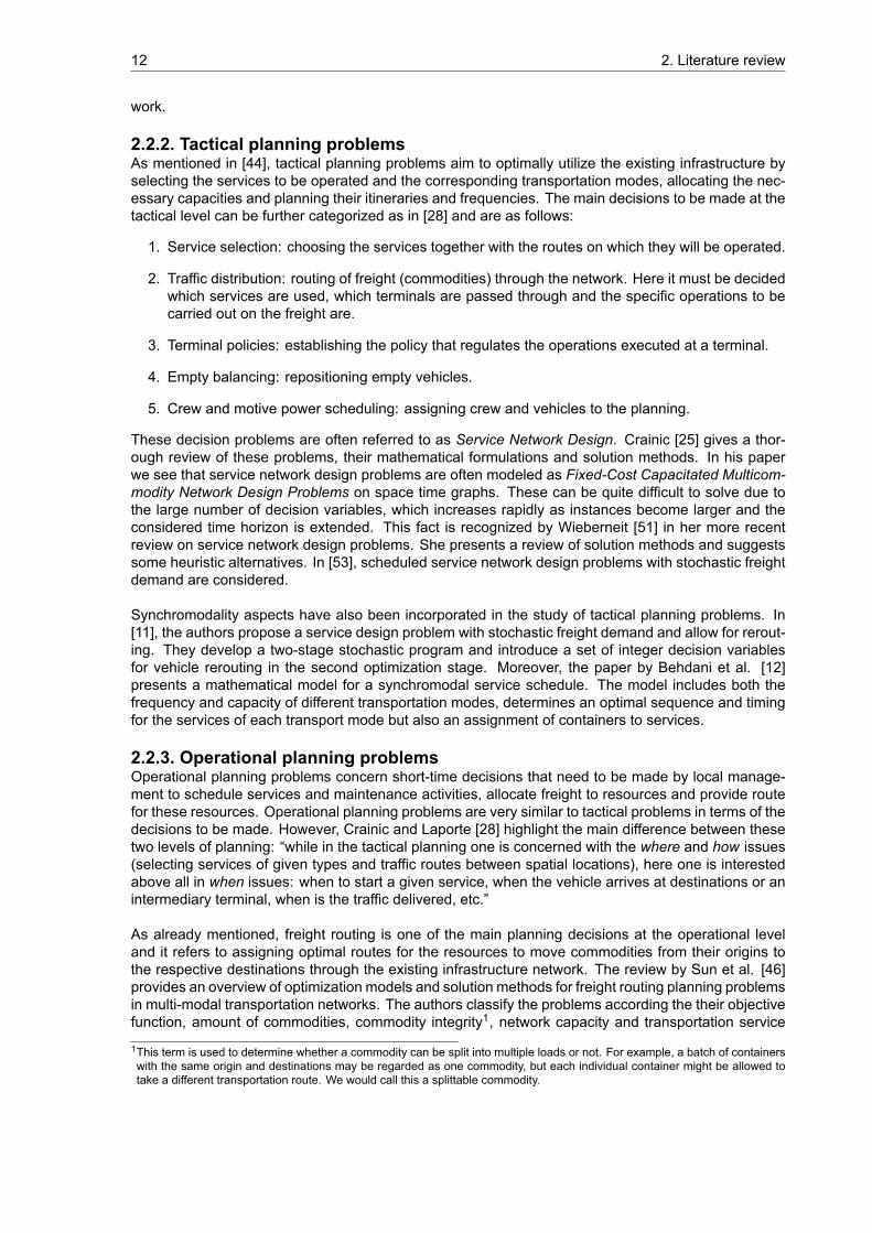
2.2.2. Tactical planning problemsAs mentioned in [44], tactical planning problems aim to optimally utilize the existing infrastructure byselecting the services to be operated and the corresponding transportation modes, allocating the nec-essary capacities and planning their itineraries and frequencies. The main decisions to be made at thetactical level can be further categorized as in [28] and are as follows:
1. Service selection: choosing the services together with the routes on which they will be operated.
2. Traffic distribution: routing of freight (commodities) through the network. Here it must be decidedwhich services are used, which terminals are passed through and the specific operations to becarried out on the freight are.
3. Terminal policies: establishing the policy that regulates the operations executed at a terminal.
4. Empty balancing: repositioning empty vehicles.
5. Crew and motive power scheduling: assigning crew and vehicles to the planning.
These decision problems are often referred to as Service Network Design. Crainic [25] gives a thor-ough review of these problems, their mathematical formulations and solution methods. In his paperwe see that service network design problems are often modeled as Fixed-Cost Capacitated Multicom-modity Network Design Problems on space time graphs. These can be quite difficult to solve due tothe large number of decision variables, which increases rapidly as instances become larger and theconsidered time horizon is extended. This fact is recognized by Wieberneit [51] in her more recentreview on service network design problems. She presents a review of solution methods and suggestssome heuristic alternatives. In [53], scheduled service network design problems with stochastic freightdemand are considered.
Synchromodality aspects have also been incorporated in the study of tactical planning problems. In[11], the authors propose a service design problem with stochastic freight demand and allow for rerout-ing. They develop a two-stage stochastic program and introduce a set of integer decision variablesfor vehicle rerouting in the second optimization stage. Moreover, the paper by Behdani et al. [12]presents a mathematical model for a synchromodal service schedule. The model includes both thefrequency and capacity of different transportation modes, determines an optimal sequence and timingfor the services of each transport mode but also an assignment of containers to services.
2.2.3. Operational planning problemsOperational planning problems concern short-time decisions that need to be made by local manage-ment to schedule services and maintenance activities, allocate freight to resources and provide routefor these resources. Operational planning problems are very similar to tactical problems in terms of thedecisions to be made. However, Crainic and Laporte [28] highlight the main difference between thesetwo levels of planning: “while in the tactical planning one is concerned with the where and how issues(selecting services of given types and traffic routes between spatial locations), here one is interestedabove all in when issues: when to start a given service, when the vehicle arrives at destinations or anintermediary terminal, when is the traffic delivered, etc.”
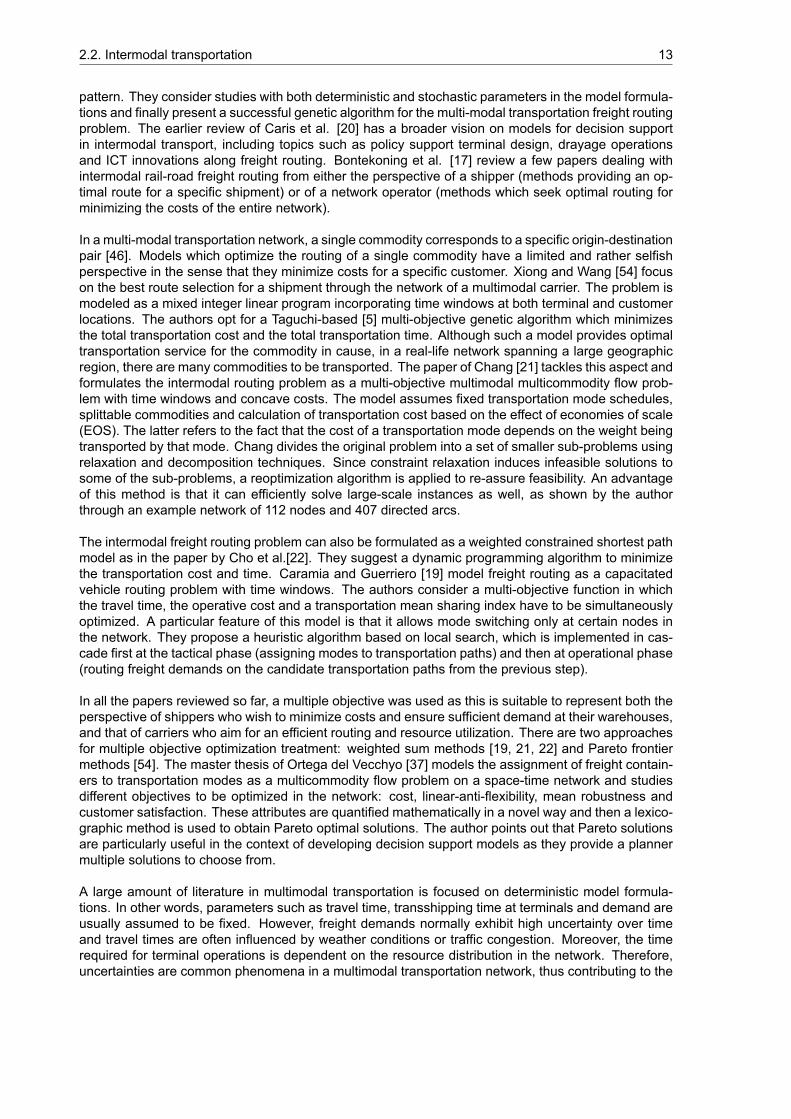
As already mentioned, freight routing is one of the main planning decisions at the operational leveland it refers to assigning optimal routes for the resources to move commodities from their origins tothe respective destinations through the existing infrastructure network. The review by Sun et al. [46]provides an overview of optimization models and solution methods for freight routing planning problemsin multi-modal transportation networks. The authors classify the problems according the their objectivefunction, amount of commodities, commodity integrity1, network capacity and transportation service
1This term is used to determine whether a commodity can be split into multiple loads or not. For example, a batch of containerswith the same origin and destinations may be regarded as one commodity, but each individual container might be allowed totake a different transportation route. We would call this a splittable commodity.
2.2. Intermodal transportation 13
pattern. They consider studies with both deterministic and stochastic parameters in the model formula-tions and finally present a successful genetic algorithm for the multi-modal transportation freight routingproblem. The earlier review of Caris et al. [20] has a broader vision on models for decision supportin intermodal transport, including topics such as policy support terminal design, drayage operationsand ICT innovations along freight routing. Bontekoning et al. [17] review a few papers dealing withintermodal rail-road freight routing from either the perspective of a shipper (methods providing an op-timal route for a specific shipment) or of a network operator (methods which seek optimal routing forminimizing the costs of the entire network).
In a multi-modal transportation network, a single commodity corresponds to a specific origin-destinationpair [46]. Models which optimize the routing of a single commodity have a limited and rather selfishperspective in the sense that they minimize costs for a specific customer. Xiong and Wang [54] focuson the best route selection for a shipment through the network of a multimodal carrier. The problem ismodeled as a mixed integer linear program incorporating time windows at both terminal and customerlocations. The authors opt for a Taguchi-based [5] multi-objective genetic algorithm which minimizesthe total transportation cost and the total transportation time. Although such a model provides optimaltransportation service for the commodity in cause, in a real-life network spanning a large geographicregion, there are many commodities to be transported. The paper of Chang [21] tackles this aspect andformulates the intermodal routing problem as a multi-objective multimodal multicommodity flow prob-lem with time windows and concave costs. The model assumes fixed transportation mode schedules,splittable commodities and calculation of transportation cost based on the effect of economies of scale(EOS). The latter refers to the fact that the cost of a transportation mode depends on the weight beingtransported by that mode. Chang divides the original problem into a set of smaller sub-problems usingrelaxation and decomposition techniques. Since constraint relaxation induces infeasible solutions tosome of the sub-problems, a reoptimization algorithm is applied to re-assure feasibility. An advantageof this method is that it can efficiently solve large-scale instances as well, as shown by the authorthrough an example network of 112 nodes and 407 directed arcs.
The intermodal freight routing problem can also be formulated as a weighted constrained shortest pathmodel as in the paper by Cho et al.[22]. They suggest a dynamic programming algorithm to minimizethe transportation cost and time. Caramia and Guerriero [19] model freight routing as a capacitatedvehicle routing problem with time windows. The authors consider a multi-objective function in whichthe travel time, the operative cost and a transportation mean sharing index have to be simultaneouslyoptimized. A particular feature of this model is that it allows mode switching only at certain nodes inthe network. They propose a heuristic algorithm based on local search, which is implemented in cas-cade first at the tactical phase (assigning modes to transportation paths) and then at operational phase(routing freight demands on the candidate transportation paths from the previous step).
In all the papers reviewed so far, a multiple objective was used as this is suitable to represent both theperspective of shippers who wish to minimize costs and ensure sufficient demand at their warehouses,and that of carriers who aim for an efficient routing and resource utilization. There are two approachesfor multiple objective optimization treatment: weighted sum methods [19, 21, 22] and Pareto frontiermethods [54]. The master thesis of Ortega del Vecchyo [37] models the assignment of freight contain-ers to transportation modes as a multicommodity flow problem on a space-time network and studiesdifferent objectives to be optimized in the network: cost, linear-anti-flexibility, mean robustness andcustomer satisfaction. These attributes are quantified mathematically in a novel way and then a lexico-graphic method is used to obtain Pareto optimal solutions. The author points out that Pareto solutionsare particularly useful in the context of developing decision support models as they provide a plannermultiple solutions to choose from.
A large amount of literature in multimodal transportation is focused on deterministic model formula-tions. In other words, parameters such as travel time, transshipping time at terminals and demand areusually assumed to be fixed. However, freight demands normally exhibit high uncertainty over timeand travel times are often influenced by weather conditions or traffic congestion. Moreover, the timerequired for terminal operations is dependent on the resource distribution in the network. Therefore,uncertainties are common phenomena in a multimodal transportation network, thus contributing to the
14 2. Literature review
complexity of freight routing problems. Uncertain parameters are often modeled as random variableswhich may have different realizations. Kooiman et. al [35] study the problem of assigning containershaving stochastic release dates to barges with fixed schedules. The release dates are assumed tohave a known uniform distribution which is dependent on their fixed due date. The authors presentpropose rule based decision making algorithms and a simulation approach. They conclude that forlarge instances, the simulation outperforms the rule based methods. The master thesis of Huizing [32]also explores the container-to-mode assignment problem assuming fixed schedules for the barges. Heformulates a multicommodity flow problem in which the travel times of the modes are assumed to benormally distributed. Two classical methods are used for removing the uncertainty from the proposedstochastic linear program namely, replacing the random variables first by their expected values andthen by pessimistic estimates of their values [36]. The results obtained were satisfactory as the solu-tions were within roughly 5% of the optimum value.
Sumalee et al. [45] study a multimodal transport network assignment with stochastic demand and sup-ply in the context of urban public transportation. Although their model might not be suitable for freighttransport, the authors describe mathematically the relationship between passengers’ waiting times atstations and weather conditions. This dependence might potentially be used for modeling terminalwaiting times. Moreover, the travel demands are assumed to follow independent Poisson distributions.The authors suggest that Lognormal andNormal distributionsmight be equally or more suitable choices.
Stochastic freight routing or more specifically, stochastic container-to-mode assignment, has alreadybeen studied in synchromodal context. Zhang and Pel [56] develop a model consisting of four com-ponents: a demand generator, a super-network processor, a schedule-based flow assignment moduleand a system performance evaluator. Transport demand is generated for a 24-hour period by randomsampling from the annual transport demand (which is known). The super-network is used to repre-sent the entire available infrastructure and schedules of transportation modes. A container-to-modeassignment is obtained by repeatedly solving a cheapest route problem. Rivera and Mes [40] study theproblems of selecting services and transfers in a synchromodal network over a multi-period horizon.The synchromodality factor is introduced here by the assumption that every transportation order canbe re-routed at any moment. Moreover, new transportation requests can enter the system during theplanning horizon. This means that new information might become available to the planner at all times.It is assumed that the planner has probabilistic knowledge about the arrival of new transportation re-quests. The authors propose a Markov Decision Process model to represent his scenario and minimizethe costs for the entire planning horizon using an approximate dynamic programming approach.
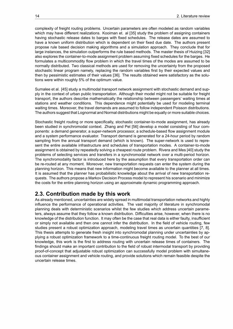
2.3. Contribution made by this workAs already mentioned, uncertainties are widely spread in multimodal transportation networks and highlyinfluence the performance of operational activities. The vast majority of literature in synchromodalplanning deals with deterministic scenarios whilst the few studies which address uncertain parame-ters, always assume that they follow a known distribution. Difficulties arise, however, when there is noknowledge of the distribution function. It may often be the case that real data is either faulty, insufficientor simply not available and then one cannot infer the distribution. In the field of vehicle routing, fewstudies present a robust optimization approach, modeling travel times as uncertain quantities [7, 8].This thesis attempts to generate fresh insight into synchromodal planning under uncertainties by ap-plying a robust optimization framework to a time-continuous freight routing model. To the best of ourknowledge, this work is the first to address routing with uncertain release times of containers. Thefindings should make an important contribution to the field of robust intermodal transport by providingproof-of-concept that adjustable robust optimization can successfully model problem with simultane-ous container assignment and vehicle routing, and provide solutions which remain feasible despite theuncertain release times.
3Overview of existing models
This chapter provides an overview of the most commonly used formulations and methods for multi-modal freight routing at operational level. One approach seems to be particularly popular namely,multicommodity flow problems. We will present our base instance in these different formulations inorder to argue how suitable they are for further encompassing more complex (uncertain) aspects.
3.1. Discrete-time multicommodity flow problemsThe studies which model multimodal freight routing as multicommodity flow problems follow either adiscrete [32] or a continuous time step approach [21]. Each of these approaches comes with its ownadvantages and drawbacks. Whilst a continuous time model enables straightforward modeling of timewindows, waiting and service time, lateness etc., a discrete approach might yield a simpler and easierto solve model since the succession of activities in time is already embodied in the network structure.We illustrate and discuss both approaches using the instance presented in section 1.2.2. Some simpli-fications or additional assumptions will be made whenever the chosen formulation cannot encompassthe complete scenario described by our base instance.
3.1.1. Theminimum costmulticommodity flow problem on a space-time networkWhen the transportation modes follow a fixed schedule and all the parameters in the network are fixed,the freight routing problem can be modeled as a minimum cost multicommodity flow problem on aspace-time graph. We provide the definition as given in [37]:
Definition 1. We call a graph 𝐺 = (𝑉, 𝐴) a space-time network (or space-time graph) if its node set 𝑉 isof the form 𝑆 × {1, 2, ..., 𝑇}, where 𝑆 represents a set of distinct locations, 𝑇 ∈ ℤ represents the amountof time steps, and every arc ((𝑎, 𝑝), (𝑏, 𝑞)) ∈ 𝐴 satisfies 𝑝 < 𝑞. We refer to the node (𝑎, 𝑝) as location𝑎 at time 𝑝, and to 𝑇 as the time horizon of 𝐺.
We can represent the available infrastructure and the fixed routes of the barges by directed arcs whichtraverse nodes describing physical locations at a particular point in time. In order to be able to furthermodel our instance as a space-time network we allow the following simplifications:
1. Assume that there is no waiting nor handling time at a terminal, namely a barge can be loadedand leave right away.
2. Assume that all containers will become available at fixed points in time.
3. Suppose that the barges will follow a fixed schedule. That is, for each barge, there is a sequenceof terminals to be visited at particular times.
4. Assume that the appointment times at customer are fixed and must always be met.
We incorporate these simplifications into our instance and model it as a space-time graph, as it canbe seen in Figure 3.1. We further elaborate on the cost structure of the network. Since barges are
15
16 3. Overview of existing models
10:00 12:30 15:00 17:30 20:00
𝐶
𝐶
𝐷
𝑇
𝑇
𝑇
𝑡
10𝑡
5
100
5
125
𝑠10
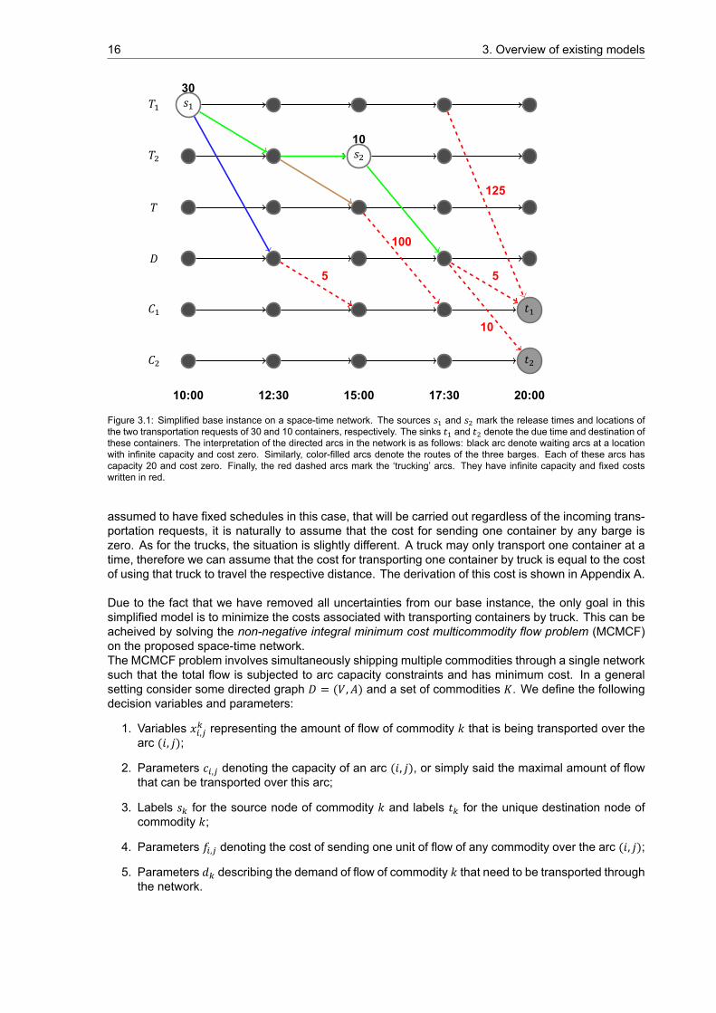
𝑠30
Figure 3.1: Simplified base instance on a space-time network. The sources and mark the release times and locations ofthe two transportation requests of 30 and 10 containers, respectively. The sinks and denote the due time and destination ofthese containers. The interpretation of the directed arcs in the network is as follows: black arc denote waiting arcs at a locationwith infinite capacity and cost zero. Similarly, color-filled arcs denote the routes of the three barges. Each of these arcs hascapacity 20 and cost zero. Finally, the red dashed arcs mark the ‘trucking’ arcs. They have infinite capacity and fixed costswritten in red.
assumed to have fixed schedules in this case, that will be carried out regardless of the incoming trans-portation requests, it is naturally to assume that the cost for sending one container by any barge iszero. As for the trucks, the situation is slightly different. A truck may only transport one container at atime, therefore we can assume that the cost for transporting one container by truck is equal to the costof using that truck to travel the respective distance. The derivation of this cost is shown in Appendix A.
Due to the fact that we have removed all uncertainties from our base instance, the only goal in thissimplified model is to minimize the costs associated with transporting containers by truck. This can beacheived by solving the non-negative integral minimum cost multicommodity flow problem (MCMCF)on the proposed space-time network.The MCMCF problem involves simultaneously shipping multiple commodities through a single networksuch that the total flow is subjected to arc capacity constraints and has minimum cost. In a generalsetting consider some directed graph 𝐷 = (𝑉, 𝐴) and a set of commodities 𝐾. We define the followingdecision variables and parameters:
1. Variables 𝑥 , representing the amount of flow of commodity 𝑘 that is being transported over thearc (𝑖, 𝑗);
2. Parameters 𝑐 , denoting the capacity of an arc (𝑖, 𝑗), or simply said the maximal amount of flowthat can be transported over this arc;
3. Labels 𝑠 for the source node of commodity 𝑘 and labels 𝑡 for the unique destination node ofcommodity 𝑘;
4. Parameters 𝑓 , denoting the cost of sending one unit of flow of any commodity over the arc (𝑖, 𝑗);
5. Parameters 𝑑 describing the demand of flow of commodity 𝑘 that need to be transported throughthe network.
3.1. Discrete-time multicommodity flow problems 17
The MCMCF problem can then be described by the following integer linear program:
min ∑( , )∈ ∑ ∈ 𝑓 , 𝑥 ,𝑠.𝑡. ∑ ∈ 𝑥 , ≤ 𝑐 , ∀(𝑖, 𝑗) ∈ 𝐴 (3.1)
∑( , )∈ 𝑥 , = 𝑑 ∀𝑘 ∈ 𝐾 (3.2)∑( , )∈ 𝑥 , = 𝑑 ∀𝑘 ∈ 𝐾 (3.3)
∑( , )∈ 𝑥 , = ∑( , )∈ 𝑥 , (∀𝑘 ∈ 𝐾)(∀𝑣 ∈ 𝑉\{𝑠 , 𝑡 }) (3.4)
𝑥 , ∈ ℕ (∀(𝑖, 𝑗) ∈ 𝐴)(∀𝑘 ∈ 𝐾) (3.5)
Constraints (3.1) assert that the total flow of commodities on any arc cannot exceed the arc capacity.Equality (3.2) states that 𝑑 units of flow of commodity 𝑘 must leave the source. Analogously, equality(3.3) assert that the total demand of commodity 𝑘 will reach its prescribed destination. Constraints (3.4)ensure flow conservation at every node in the network. Finally, the last set of constraints require thatany amount of flow of any commodity to be transported must be a positive integer. These constraintsemerge from the fact that we identify one unit of flow with one container. One can now understand thatthe optimal container-to-mode assignment is an instance of the MCMCF problem and its correspond-ing integer linear program can be solved with the aid of a solver. The solution thus obtained for thesimplified base instance is shown in Figure 3.2.
10:00 12:30 15:00 17:30 20:00
𝐶
𝐶
𝐷
𝑇
𝑇
𝑇
𝑡
10𝑡
5
100
5
125
𝑠10
𝑠30
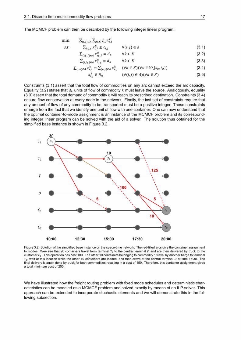
Figure 3.2: Solution of the simplified base instance on the space-time network. The red-filled arcs give the container assignmentto modes. Wee see that 20 containers travel from terminal to the central terminal and are then delivered by truck to thecustomer . This operation has cost 100. The other 10 containers belonging to commodity 1 travel by another barge to terminal, wait at this location while the other 10 containers are loaded, and then arrive at the central terminal at time 17:30. The
final delivery is again done by truck for both commodities resulting in a cost of 150. Therefore, this container assignment givesa total minimum cost of 250.
We have illustrated how the freight routing problem with fixed mode schedules and deterministic char-acteristics can be modeled as a MCMCF problem and solved exactly by means of an ILP solver. Thisapproach can be extended to incorporate stochastic elements and we will demonstrate this in the fol-lowing subsection.
18 3. Overview of existing models
3.1.2. Theminimumcostmulticommodity flow problemwith stochastic elementsThe previous arc-based formulation of the MCMCF problem on a space-time network may also includeuncertainty in the transportation data in the form of stochastic parameters. As a simple example, weconsider an incoming order of containers at a deep-sea terminal, that needs to be picked up by oneof the barges of the logistics service provider. The exact time at which these containers will becomeavailable for pick-up is not known. However, the planner has some probabilistic knowledge of theserelease times. Therefore, one needs to address the problem of assigning containers to barges whichfollow fixed schedules, given that the release times of these containers follow known distributions. Weillustrate this scenario in Figure 3.3, with the aid of a slightly adjusted version of the instance shown inFigure 3.1. Since the source node of commodity 1 is essentially modeled as a random variable with
7:30 10:00 12:30 15:00 17:30 20:00
𝐶
𝐶
𝐷
𝑇
𝑇
𝑇
𝑡
10𝑡
5
100
5
125
𝑠10
𝑠30?
𝑠30?
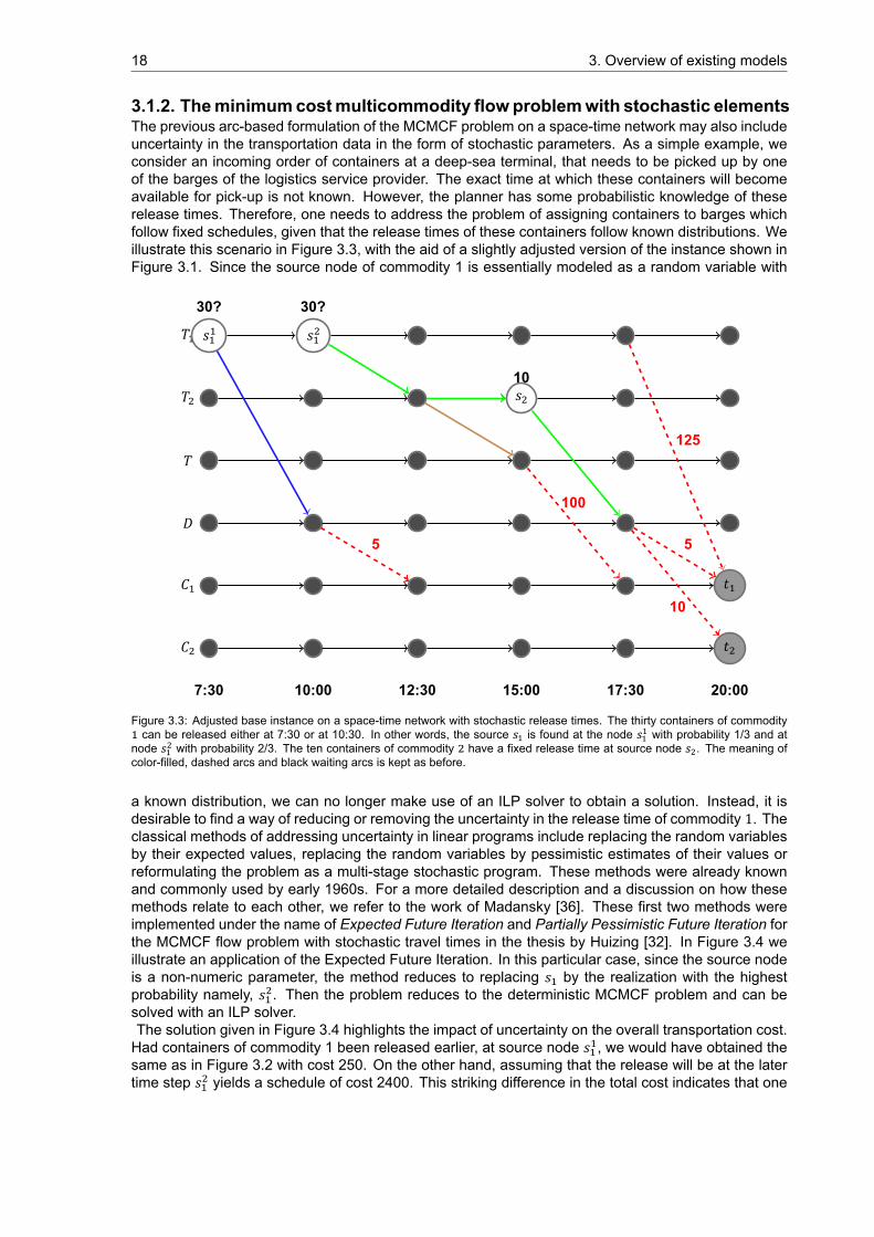
Figure 3.3: Adjusted base instance on a space-time network with stochastic release times. The thirty containers of commoditycan be released either at 7:30 or at 10:30. In other words, the source is found at the node with probability 1/3 and at
node with probability 2/3. The ten containers of commodity have a fixed release time at source node . The meaning ofcolor-filled, dashed arcs and black waiting arcs is kept as before.
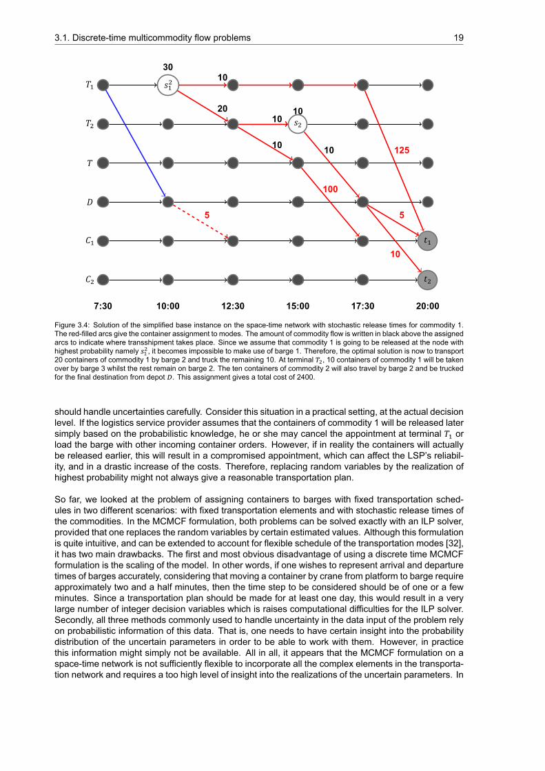
a known distribution, we can no longer make use of an ILP solver to obtain a solution. Instead, it isdesirable to find a way of reducing or removing the uncertainty in the release time of commodity 1. Theclassical methods of addressing uncertainty in linear programs include replacing the random variablesby their expected values, replacing the random variables by pessimistic estimates of their values orreformulating the problem as a multi-stage stochastic program. These methods were already knownand commonly used by early 1960s. For a more detailed description and a discussion on how thesemethods relate to each other, we refer to the work of Madansky [36]. These first two methods wereimplemented under the name of Expected Future Iteration and Partially Pessimistic Future Iteration forthe MCMCF flow problem with stochastic travel times in the thesis by Huizing [32]. In Figure 3.4 weillustrate an application of the Expected Future Iteration. In this particular case, since the source nodeis a non-numeric parameter, the method reduces to replacing 𝑠 by the realization with the highestprobability namely, 𝑠 . Then the problem reduces to the deterministic MCMCF problem and can besolved with an ILP solver.The solution given in Figure 3.4 highlights the impact of uncertainty on the overall transportation cost.Had containers of commodity 1 been released earlier, at source node 𝑠 , we would have obtained thesame as in Figure 3.2 with cost 250. On the other hand, assuming that the release will be at the latertime step 𝑠 yields a schedule of cost 2400. This striking difference in the total cost indicates that one
3.1. Discrete-time multicommodity flow problems 19
7:30 10:00 12:30 15:00 17:30 20:00
𝐶
𝐶
𝐷
𝑇
𝑇
𝑇
𝑡
10𝑡
5
100
5
10 125
𝑠1010
10
10
20
𝑠30
Figure 3.4: Solution of the simplified base instance on the space-time network with stochastic release times for commodity 1.The red-filled arcs give the container assignment to modes. The amount of commodity flow is written in black above the assignedarcs to indicate where transshipment takes place. Since we assume that commodity 1 is going to be released at the node withhighest probability namely , it becomes impossible to make use of barge 1. Therefore, the optimal solution is now to transport20 containers of commodity 1 by barge 2 and truck the remaining 10. At terminal , 10 containers of commodity 1 will be takenover by barge 3 whilst the rest remain on barge 2. The ten containers of commodity 2 will also travel by barge 2 and be truckedfor the final destination from depot . This assignment gives a total cost of 2400.
should handle uncertainties carefully. Consider this situation in a practical setting, at the actual decisionlevel. If the logistics service provider assumes that the containers of commodity 1 will be released latersimply based on the probabilistic knowledge, he or she may cancel the appointment at terminal 𝑇 orload the barge with other incoming container orders. However, if in reality the containers will actuallybe released earlier, this will result in a compromised appointment, which can affect the LSP’s reliabil-ity, and in a drastic increase of the costs. Therefore, replacing random variables by the realization ofhighest probability might not always give a reasonable transportation plan.
So far, we looked at the problem of assigning containers to barges with fixed transportation sched-ules in two different scenarios: with fixed transportation elements and with stochastic release times ofthe commodities. In the MCMCF formulation, both problems can be solved exactly with an ILP solver,provided that one replaces the random variables by certain estimated values. Although this formulationis quite intuitive, and can be extended to account for flexible schedule of the transportation modes [32],it has two main drawbacks. The first and most obvious disadvantage of using a discrete time MCMCFformulation is the scaling of the model. In other words, if one wishes to represent arrival and departuretimes of barges accurately, considering that moving a container by crane from platform to barge requireapproximately two and a half minutes, then the time step to be considered should be of one or a fewminutes. Since a transportation plan should be made for at least one day, this would result in a verylarge number of integer decision variables which is raises computational difficulties for the ILP solver.Secondly, all three methods commonly used to handle uncertainty in the data input of the problem relyon probabilistic information of this data. That is, one needs to have certain insight into the probabilitydistribution of the uncertain parameters in order to be able to work with them. However, in practicethis information might simply not be available. All in all, it appears that the MCMCF formulation on aspace-time network is not sufficiently flexible to incorporate all the complex elements in the transporta-tion network and requires a too high level of insight into the realizations of the uncertain parameters. In
20 3. Overview of existing models
the next subsection, we look into time-continuous models in order to allow for a better representationof the time parameters in the transportation network.
3.2. Multicommodity flow problemswith continuous time variablesWe have already established that the treatment of time is an important aspect in container routingproblems. As the discrete-time models presented in the previous section were shown to be too limitedto exploit in the context of a transportation network with uncertainties, we will now focus on findingtime-continuous approaches, which are expected to be more suitable for modeling our base instance.
3.2.1. Multicommodity scheduled service network designIn her doctoral thesis, Sharypova [41] studies the problem of scheduled service network design forcontainer freight transportation along inland waterways. She proposes a continuous-time mixed in-teger linear programming model which takes as input the transportation network, the available fleetof vehicles, the demand and supply of containers, the sailing time of vehicles, and the structure ofcosts, and provides a minimum cost container distribution plan together with a vehicle and containerrouting schedule. This service design formulation is intended for usage at a tactical level but can bere-interpreted to also serve short-term planning at operational level. We will present a slightly adjustedversion of the model as given in [41], with the exception that some of the additional costs for vehicleutilization and handling activities at terminals have been removed.
Let 𝐺 = (𝑉, 𝐴) denote a directed graph describing the transportation network. The vertex set 𝑉 corre-sponds to the set of physical locations in our base instance namely {𝑇 , 𝑇 , 𝑇, 𝐷, 𝐶 , 𝐶 }, whilst and arc(𝑖, 𝑗) in the set 𝐴 marks a direct1 trip between the physical locations 𝑖 and 𝑗. We denote by 𝑀 the setof vehicles and by 𝐾 the set of commodities. It is important to mention that a commodity is defined asa set of containers which have the same origin, destination, release time at the origin and due time atdestination. We let 𝐷 represent the number of containers in commodity 𝑘 that need to be transportedfrom the node of its origin the its destination. Furthermore, consider the following input parameters:
• 𝑐 , : unit transportation cost paid to transport one container by vehicle 𝑚 ∈ 𝑀;
• ℎ : unit handling cost at location 𝑖 ∈ 𝑉;
• 𝑠 : service time at node 𝑖 ∈ 𝑉;
• 𝑑 : demand of commodity 𝑘 ∈ 𝐾 at node 𝑖 ∈ 𝑉;
• (𝑜(𝑘), 𝑑(𝑘)): origin-destination node pair of commodity 𝑘 ∈ 𝐾;
• 𝑟 : release time of commodity 𝑘 ∈ 𝐾 at its origin;
• 𝑑𝑢𝑒 : due time of commodity 𝑘 ∈ 𝐾 at its final destination;
• 𝑡 , : traveling time of vehicle 𝑚 ∈ 𝑀 from node 𝑖 ∈ 𝑉 to node 𝑗 ∈ 𝑉;
• 𝑐 : maximum capacity of vehicle 𝑚 ∈ 𝑀.
In particular, we define the demand of commodity 𝑘 at node 𝑖 in the following way:
𝑑 = {𝐷 if 𝑖 = 𝑜(𝑘)−𝐷 if 𝑖 = 𝑑(𝑘)0 otherwise
All the parameters described above will have a known fixed value except for the release times 𝑟 . Weassume that for every commodity 𝑘 ∈ 𝐾, its release time lies in a bounded interval, namely 𝑟 ∈ [𝑙 , 𝑢 ]where the values of the bounds 𝑙 and 𝑢 are known. The set 𝑉 ⊂ 𝑉 represents the subset of locationswhich are accessible by vehicle 𝑚.
1We refer to a trip of a vehicle with no intermediate stops as a direct trip.
3.2. Multicommodity flow problems with continuous time variables 21
The following decision variables are introduced:
• 𝑥 ,, : integer variable describing number of containers of commodity 𝑘 ∈ 𝐾 transported from
location 𝑖 ∈ 𝑉 to location 𝑗 ∈ 𝑉 by vehicle 𝑚 ∈ 𝑀;
• 𝑦 , : binary variable which takes value 1 if vehicle 𝑚 ∈ 𝑀 travels from location 𝑖 ∈ 𝑉 to location𝑗 ∈ 𝑉 and 0 otherwise;
• 𝑧 : binary variable which takes value 1 is vehicle 𝑚 ∈ 𝑀 is used in the transportation plan and 0otherwise;
• 𝐴 : continuous variable describing the arrival time of vehicle 𝑚 ∈ 𝑀 at location 𝑖 ∈ 𝑉;
• 𝐷 : continuous variable describing the departure time of vehicle 𝑚 ∈ 𝑀 from location 𝑖 ∈ 𝑉;
• 𝑞 , , : continuous variable describing the amount of containers of commodity 𝑘 ∈ 𝐾 moved fromvehicle 𝑚 ∈ 𝑀 to vehicle 𝑙 ∈ 𝑀 at location 𝑖 ∈ 𝑉 ∩ 𝑉 ;
• 𝜃 , : binary variable which takes value 1 if a transshipment occurs between vehicle 𝑚 ∈ 𝑀 andvehicle 𝑙 ∈ 𝑀 at location 𝑖 ∈ 𝑉 ∩ 𝑉 ;
• 𝜏 , : binary variable which takes value 1 if any container of commodity 𝑘 ∈ 𝐾 is loaded on vehicle𝑚 ∈ 𝑀 at node 𝑖 ∈ {𝑜(𝑘), 𝑑(𝑘)}.
We further denote the set of outgoing arcs from node 𝑖 ∈ 𝑉 by 𝑉 (𝑖), and the set of ingoing arcs by𝑉 (𝑖). Given these parameters and decision variables, the container routing problem can be formulatedas the following mixed integer program:
min ∑ ∈ ∑ ∈ ∑( , )∈ 𝑐 , 𝑥 ,,
𝑠.𝑡. ∑( )∈ ( ) 𝑦 , − ∑ ∈ ( ) 𝑦 , = 0 ∀𝑚 ∈ 𝑀,∀𝑖 ∈ 𝑉 (3.6)
∑ ∈ ∑ ∈ ( ) 𝑥 ,, − ∑ ∈ ∑ ∈ ( ) 𝑥 ,
, = 𝑑 ∀𝑖 ∈ 𝑉, ∀𝑘 ∈ 𝐾 (3.7)
∑ ∈ 𝑥 ,, ≤ 𝑐 𝑦 , ∀𝑚 ∈ 𝑀,∀(𝑖, 𝑗) ∈ 𝐴 (3.8)
∑ ∈ 𝑞 , , > 0 ⟺ 𝜃 , = 1 ∀𝑚, 𝑙 ∈ 𝐾, ∀𝑖 ∈ 𝑉 ∩ 𝑉 (3.9)∑ ∈ ( ) 𝑥 ,
, = ∑ ∈ 𝑞 , , ∀𝑚 ∈ 𝑀,∀𝑘 ∈ 𝐾, ∀𝑖 ∈ 𝑉 ⧵ {𝑑(𝑘)} (3.10)
∑ ∈ ( ) 𝑥 ,, = ∑ ∈ 𝑞 , , ∀𝑚 ∈ 𝑀,∀𝑘 ∈ 𝐾, ∀𝑖 ∈ 𝑉 ⧵ {𝑜(𝑘)} (3.11)
∑ ∈ 𝑞 , , = 0 ∀𝑚 ∈ 𝑀,∀𝑘 ∈ 𝐾, ∀𝑖 ∈ {𝑜(𝑘), 𝑑(𝑘)} (3.12)∑ ∈ ( ) 𝑥 ,
, > 0 ⟺ 𝜏 , = 1 ∀𝑚 ∈ 𝑀,∀𝑘 ∈ 𝐾, ∀𝑖 ∈ {𝑜(𝑘)} (3.13)
∑ ∈ ( ) 𝑥 ,, > 0 ⟺ 𝜏 , = 1 ∀𝑚 ∈ 𝑀,∀𝑘 ∈ 𝐾, ∀𝑖 ∈ {𝑑(𝑘)} (3.14)
𝜃 , = 1 ⇒ 𝐷 − 𝐴 − 𝑠 ≥ 0 ∀𝑚, 𝑙 ∈ 𝑀, ∀𝑖 ∈ 𝑉 ∩ 𝑉 (3.15)𝑦 , ⇒ 𝐷 + 𝑡 , − 𝐴 ≤ 0 ∀𝑚 ∈ 𝑀,∀(𝑖, 𝑗) ∈ 𝐴 (3.16)
𝐷 ≥ 𝐴 + 𝑠 ∀𝑚 ∈ 𝑀,∀𝑖 ∈ 𝑉 (3.17)𝐷 ≥ 𝑟 𝜏 , ∀𝑘 ∈ 𝐾, ∀𝑖 ∈ {𝑜(𝑘)}, ∀𝑚 ∈ 𝑀 (3.18)
𝜏 , ⇒ 𝐴 ≤ 𝑑𝑢𝑒 ∀𝑘 ∈ 𝐾, ∀𝑖 ∈ {𝑑(𝑘)}, ∀𝑚 ∈ 𝑀 (3.19)∑ ∈ ( ) 𝑦 , ≤ 𝑧 ∀𝑚 ∈ 𝑀,∀𝑖 ∈ 𝑉 (3.20)
𝑥 ,, ∈ ℕ ∀𝑚 ∈ 𝑀,∀(𝑖, 𝑗) ∈ 𝐴, ∀𝑘 ∈ 𝐾 (3.21)
𝑞 , , ∈ ℕ ∀𝑚, 𝑙 ∈ 𝑀, ∀𝑖 ∈ 𝑉 ∩ 𝑉, ∀𝑘 ∈ 𝐾 (3.22)𝐴 ,𝐷 ≥ 0 ∀𝑚 ∈ 𝑀,∀𝑖 ∈ 𝑉 (3.23)𝑦 , ∈ {0, 1} ∀𝑚 ∈ 𝑀, ∀(𝑖, 𝑗) ∈ 𝐴 (3.24)
𝜃 , ∈ {0, 1} ∀𝑚, 𝑙 ∈ 𝑀, ∀𝑖 ∈ 𝑉 ∩ 𝑉 (3.25)𝜏 , ∈ {0, 1} ∀𝑘 ∈ 𝐾, ∀𝑚 ∈ 𝑀, ∀𝑖 ∈ {𝑜(𝑘), 𝑑(𝑘)} (3.26)𝑧 ∈ {0, 1} ∀𝑚 ∈ 𝑀 (3.27)
22 3. Overview of existing models
In order to describe the practical meaning of the (in)equalities above in a more efficient way, we willcategorize them.
Objective function: The sum of transportation costs for all the containers is to be minimized.
Flow conservation constraints: Constraints (3.6) assert that a vehicle which is arriving at a locationin the network, should also leave that location afterwards. Constraints (3.7) ensure that the demand ofcommodities is satisfied at every node in the network.
Vehicle capacity: Constraints (3.8) indicate that the amount of flow transported by a vehicle on anyarc should not exceed the maximum capacity of the vehicle.
Transshipment conditions: Constraints (3.9) assert that there is transshipment from vehicle 𝑚 tovehicle 𝑙 if only only if there exist some containers to be moved from vehicle 𝑚 to vehicle 𝑙. Theseconstraints can be written in the following linearized form:
∑∈𝑞 , , ≥ 𝑀 (1 − 𝜃 , ) + 𝜖 ∀𝑚, 𝑙 ∈ 𝐾, ∀𝑖 ∈ 𝑉 ∩ 𝑉 (3.28)
∑∈𝑞 , , ≤ 𝑀 𝜃 , ∀𝑚, 𝑙 ∈ 𝐾, ∀𝑖 ∈ 𝑉 ∩ 𝑉 (3.29)
with 𝑀 being a large positive integer and 𝜖 a small positive constant. Typically, one may consider𝑀 = 1000 and 𝜖 = 10 . The equality in (3.10) describe what happens to containers of a certaincommodity once they arrive at a location (which logically should not be their final destination since theirtrip ends here). That is, all containers of the same commodity 𝑘 brought by vehicle 𝑚 to location 𝑖should either be moved to other vehicles (𝑚 ≠ 𝑙) or remain on board of vehicle 𝑚 (𝑚 = 𝑙). Similarly,constraints (3.11) guarantee that upon their departure from node 𝑖, all containers of the same commod-ity are either transshipped to another vehicle, or continue their journey on the same vehicle 𝑚 whichoriginally brought them to 𝑖. Constraints (3.12) enforce that there is no transshipment possible at theorigin and destination node of any commodity.
Commodity flow at origin and destination: Constraints (3.13) describe the fact that a container ofcommodity 𝑘 can be on board of vehicle𝑚 at its origin node 𝑜(𝑘) if and only if the amount of containerswhich have left this node on board of vehicle 𝑚 is positive. Analogously, constraints (3.14) states thatif there is a positive flow of commodity 𝑘 arriving at their destination on vehicle 𝑚, then this commodityis on board of vehicle 𝑚 at node 𝑑(𝑘). We can linearize these conditions by the following inequalities:
∑∈ ( )
𝑥 ,, ≥ 𝑀 (𝜏 , − 1) + 𝜖 ∀𝑚 ∈ 𝑀,∀𝑘 ∈ 𝐾, ∀𝑖 ∈ {𝑜(𝑘)} (3.30)
∑∈ ( )
𝑥 ,, ≤ 𝑀 𝜏 , ∀𝑚 ∈ 𝑀,∀𝑘 ∈ 𝐾, ∀𝑖 ∈ {𝑜(𝑘)} (3.31)
∑∈ ( )
𝑥 ,, ≥ 𝑀 (𝜏 , − 1) + 𝜖 ∀𝑚 ∈ 𝑀,∀𝑘 ∈ 𝐾, ∀𝑖 ∈ {𝑑(𝑘)} (3.32)
∑∈ ( )
𝑥 ,, ≤ 𝑀 𝜏 , ∀𝑚 ∈ 𝑀,∀𝑘 ∈ 𝐾, ∀𝑖 ∈ {𝑑(𝑘)}, (3.33)
where 𝑀 and 𝜖 have the same meaning as before.
Vehicle synchronization for transshipment: Constraints (3.15) indicate that if there is a movementof containers from vehicle 𝑚 to vehicle 𝑙 at node 𝑖, then vehicle 𝑙 may only depart with the loaded com-modity if this has been already brought to node 𝑖 by vehicle 𝑚. The linear version of this constraints isas follows:
𝐷 − 𝐴 − 𝑠 ≥ 𝑀 (𝜃 , − 1) ∀𝑚, 𝑙 ∈ 𝑀, ∀𝑖 ∈ 𝑉 ∩ 𝑉. (3.34)
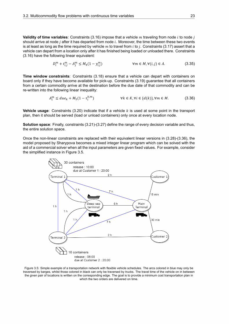
3.2. Multicommodity flow problems with continuous time variables 23
Validity of time variables: Constraints (3.16) impose that a vehicle 𝑚 traveling from node 𝑖 to node 𝑗should arrive at node 𝑗 after it has departed from node 𝑖. Moreover, the time between these two eventsis at least as long as the time required by vehicle𝑚 to travel from 𝑖 to 𝑗. Constraints (3.17) assert that avehicle can depart from a location only after it has finished being loaded or unloaded there. Constraints(3.16) have the following linear equivalent:
𝐷 + 𝑡 , − 𝐴 ≤ 𝑀 (1 − 𝑦 , ) ∀𝑚 ∈ 𝑀, ∀(𝑖, 𝑗) ∈ 𝐴. (3.35)
Time window constraints: Constraints (3.18) ensure that a vehicle can depart with containers onboard only if they have become available for pick-up. Constraints (3.19) guarantee that all containersfrom a certain commodity arrive at the destination before the due date of that commodity and can bere-written into the following linear inequality:
𝐴 ≤ 𝑑𝑢𝑒 +𝑀 (1 − 𝜏 , ) ∀𝑘 ∈ 𝐾, ∀𝑖 ∈ {𝑑(𝑘)}, ∀𝑚 ∈ 𝑀. (3.36)
Vehicle usage: Constraints (3.20) indicate that if a vehicle 𝑘 is used at some point in the transportplan, then it should be served (load or unload containers) only once at every location node.
Solution space: Finally, constraints (3.21)-(3.27) define the range of every decision variable and thus,the entire solution space.
Once the non-linear constraints are replaced with their equivalent linear versions in (3.28)-(3.36), themodel proposed by Sharypova becomes a mixed integer linear program which can be solved with theaid of a commercial solver when all the input parameters are given fixed values. For example, considerthe simplified instance in Figure 3.5.
Figure 3.5: Simple example of a transportation network with flexible vehicle schedules. The arcs colored in blue may only betraversed by barges, whilst those colored in black can only be traversed by trucks. The travel time of the vehicle on in betweenthe given pair of locations is written on the corresponding edge. The goal is to provide a minimum cost transportation plan in
which the two orders are delivered on time.

24 3. Overview of existing models
In this example, there are two transportation requests that must be carried out from their origin to theirdestination before their due time. There are three barges of capacity 20 situated at the Deep sea termi-nal, along with a sufficiently large number of trucks with capacity 1 available at both the Main Terminaland the Deep sea terminal. We assume that all vehicles are available for utilization well before the firstcontainers are released and that at every location there is a uniform service time of one hour. Thereare no costs for traveling by barge. However, every truck-arc has a cost associated which is definedas follows: the two arcs from the Main Terminal to the Customers have costs equal to 5. Each of therest of the truck arcs has a cost of 10. Solving the mixed integer linear program described earlier withthis particular set of parameters yields an optimal schedule of total cost equal to 200. The assignmentof containers is as follows: twenty containers from Terminal 1 are carried by one barge to the MainTerminal and further trucked to Customer 1. Another barge will handle the ten remaining containersand bring them to the Main Terminal, from which they will be trucked. Finally, a third barge will transportthe ten containers released at Terminal 2, bringing them to the Main Terminal. Again, the last leg ofthe trip to the final customer destination is done by trucks. As a result of this transportation plan, allthirty containers of the first order arrive at their destination at 18:15, whilst the rest of ten containerscorresponding to the second order, reach their destination at 18:30.
We observe that in the optimal solution three barges must be used to meet the strict deadlines ofthe transportation orders. Had these deadlines been scheduled at a later moment, one could havecarried the total load of forty containers with only two barges. Although in our base instance this aspectgoes unnoticed since we have not defined arc costs for the barges, using one vehicle less can yielda big cost reduction in practice. Moreover, in the logistics reality, it may often occur that the penaltyinquired for being late with servicing a customer is not nearly as high as the cost incurred for utilizingmore vehicles. Therefore, it is important to allow for flexibility in meeting the appointment times at thedestinations of shipments and to model overall costs appropriately, seeking to reflect as much as pos-sible their impact in a real transportation network.
Although the model proposed by Sharypova includes fixed deadlines at customers and does not al-low for multiple visits of a vehicle at a location, it incorporates flexible schedules for the transportationmodes and time variables which record the start and end time of all the transport activities in the net-work. Aspects such as service time at a location, waiting time, and actual travel time are very easy tomodel with this approach. Moreover, within the larger scope of dealing with uncertainty in the trans-port parameters, there is a great body of literature related to solution methods for mixed integer linearprograms with uncertain data. Concerning scalability, this mixed integer program can solve exactlyinstances with up to fifty commodities. All in all, it appears that this model is a suitable choice fordescribing our base instance, possibly extending it and solving it to obtain a transportation plan.
3.2.2. Multicommodity bulk shippingWhen studying modeling approaches for freight transportation, it is worthwhile to also consider liquidbulk logistics. This refers to the problem of routing a fleet of vessels engaged in the pick-up anddelivery of different liquid bulk products, which is often encountered by oil companies. Liquids areconsidered bulk cargo, and can be described as commodities that cannot be handled as individualpieces. Although in terms of capacity, handling of commodities and overall objective, these problemsare very different from freight routing, some aspects of the transport network still remain very similar,and as a consequence, the models are often built on the same kind of networks and impose the sameconstraints (flow conservation, timely arrival at customer locations etc.). In essence, liquid bulk routingproblems can give new insights into modeling techniques that might counter some assumptions in thefreight routing formulations. In this regard, we recall that the model of Sharypova did not allow formultiple visits of a vehicle at a location. However, this assumption is not realistic and is discussed byAl-Khayyal and Hwang [9]. They propose a model for finding a minimum cost routing in a network for afleet of vessels carrying liquid products. The highlight of their work is the actual design of the networknamely, a node (𝑖,𝑚) in the network, where 𝑖 denotes the location and 𝑚 marks the arrival number ofthat location within the planning horizon. An example is shown in Figure 3.6.
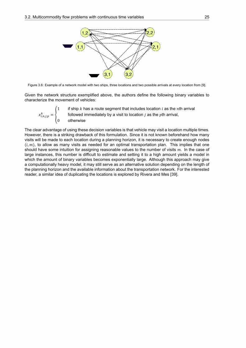
3.2. Multicommodity flow problems with continuous time variables 25
Figure 3.6: Example of a network model with two ships, three locations and two possible arrivals at every location from [9].
Given the network structure exemplified above, the authors define the following binary variables tocharacterize the movement of vehicles:
𝑥 , , , = {1 if ship 𝑘 has a route segment that includes location 𝑖 as the 𝑛th arrival
followed immediately by a visit to location 𝑗 as the 𝑝th arrival,0 otherwise
The clear advantage of using these decision variables is that vehicle may visit a location multiple times.However, there is a striking drawback of this formulation. Since it is not known beforehand how manyvisits will be made to each location during a planning horizon, it is necessary to create enough nodes(𝑖,𝑚), to allow as many visits as needed for an optimal transportation plan. This implies that oneshould have some intuition for assigning reasonable values to the number of visits 𝑚. In the case oflarge instances, this number is difficult to estimate and setting it to a high amount yields a model inwhich the amount of binary variables becomes exponentially large. Although this approach may givea computationally heavy model, it may still serve as an alternative solution depending on the length ofthe planning horizon and the available information about the transportation network. For the interestedreader, a similar idea of duplicating the locations is explored by Rivera and Mes [39].


4Deterministic problem formulation
In this chapter we present a mathematical model for the freight routing problem described as our baseinstance. We will use Sharypova’s model [41] as the basis of our research and further develop it toincorporate all aspects which are of interest in the context of uncertain parameters in the transportationnetwork. In Section 4.1 we describe all the modifications brought to the original mixed integer linearprogram. In Section 4.2 we elaborate on a further extension of themodel that can be used to incorporatemultiple trips of a vehicle to a certain location.
4.1. Deterministic modelSharypova’s model [41] serves as a starting point in our problem formulation. This model provides atransportation schedule of minimum cost which meets the strict delivery deadlines at the destinationsof commodities. Since our goal is to investigate the impact of uncertainty on the transportation plan,it is reasonable to allow for more flexibility in the network namely, replace the strict deadlines of com-modities by the so-called soft due times. This implies that a commodity may arrive later than its duedate at its destination, in which case a penalty cost is incurred. To model this aspect, we introducelateness decision variables 𝐿 , describing how late vehicle 𝑚 is at location 𝑖. Clearly, these variablesare only defined when location 𝑖 is a destination node for some commodity. Moreover, in our baseinstance described in section 1.2.2, we assumed that a barge arriving at a deep-sea terminal must waita certain amount of time before it starts being loaded or unloaded. Thus, we will incorporate a terminalspecific parameter 𝑤 , representing the amount of time that a barge has to wait at terminal 𝑖. Finally,the components of the objective function must be addressed.
Whilst in Chapter 3 we discussed an objective function related to vehicle utilization, transportationand handling costs, in our case the focus will be on time related components. Generally speaking,we are interested in minimizing the utilization of trucks. However, in practice it is often the case thattrucks and trails are rented by the hour and motivated by this, we will aim for minimizing the truckinghours. A trucking hour is one hour in which a truck has been utilized for transportation purposes. It isimportant to remark here that the amount of trucks used overall or the time traveled by a truck withoutbeing loaded are not important quantities in this setting. Moreover, we complete our multi-objectivefunction by incorporating the total lateness recorded in the planning. This term quantifies by how muchtime container arrivals differ from their specified due date. Weights are associated with each of the twoobjectives for scaling purposes. These weights allow us to prioritize one objective over the other one,as in practice one might often find that arriving an hour late at a location might be preferable to rentinga truck for another hour. A thorough discussion on these weights will follow in Chapter 6.
27
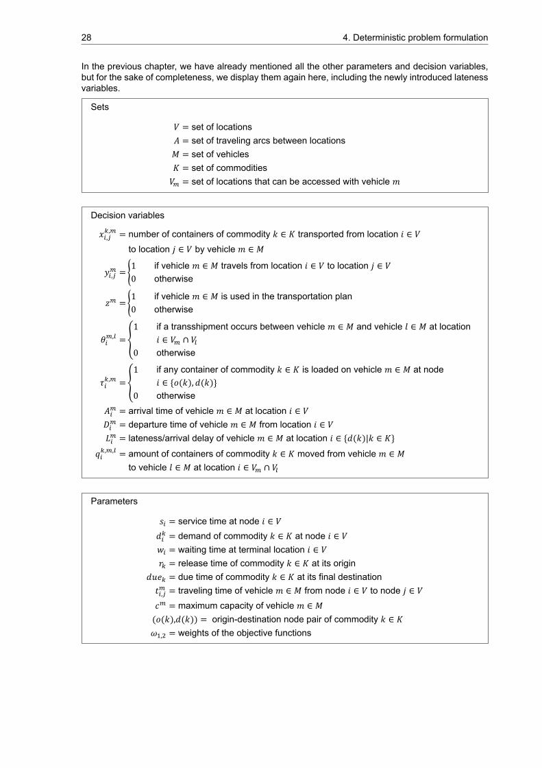
28 4. Deterministic problem formulation
In the previous chapter, we have already mentioned all the other parameters and decision variables,but for the sake of completeness, we display them again here, including the newly introduced latenessvariables.
Sets
𝑉 = set of locations𝐴 = set of traveling arcs between locations𝑀 = set of vehicles𝐾 = set of commodities𝑉 = set of locations that can be accessed with vehicle 𝑚
Decision variables
𝑥 ,, = number of containers of commodity 𝑘 ∈ 𝐾 transported from location 𝑖 ∈ 𝑉
to location 𝑗 ∈ 𝑉 by vehicle 𝑚 ∈ 𝑀
𝑦 , ={1 if vehicle 𝑚 ∈ 𝑀 travels from location 𝑖 ∈ 𝑉 to location 𝑗 ∈ 𝑉0 otherwise
𝑧 = {1 if vehicle 𝑚 ∈ 𝑀 is used in the transportation plan0 otherwise
𝜃 , ={1 if a transshipment occurs between vehicle 𝑚 ∈ 𝑀 and vehicle 𝑙 ∈ 𝑀 at location
𝑖 ∈ 𝑉 ∩ 𝑉0 otherwise
𝜏 , ={1 if any container of commodity 𝑘 ∈ 𝐾 is loaded on vehicle 𝑚 ∈ 𝑀 at node
𝑖 ∈ {𝑜(𝑘), 𝑑(𝑘)}0 otherwise
𝐴 = arrival time of vehicle 𝑚 ∈ 𝑀 at location 𝑖 ∈ 𝑉𝐷 = departure time of vehicle 𝑚 ∈ 𝑀 from location 𝑖 ∈ 𝑉𝐿 = lateness/arrival delay of vehicle 𝑚 ∈ 𝑀 at location 𝑖 ∈ {𝑑(𝑘)|𝑘 ∈ 𝐾}
𝑞 , , = amount of containers of commodity 𝑘 ∈ 𝐾 moved from vehicle 𝑚 ∈ 𝑀to vehicle 𝑙 ∈ 𝑀 at location 𝑖 ∈ 𝑉 ∩ 𝑉
Parameters
𝑠 = service time at node 𝑖 ∈ 𝑉𝑑 = demand of commodity 𝑘 ∈ 𝐾 at node 𝑖 ∈ 𝑉𝑤 = waiting time at terminal location 𝑖 ∈ 𝑉𝑟 = release time of commodity 𝑘 ∈ 𝐾 at its origin
𝑑𝑢𝑒 = due time of commodity 𝑘 ∈ 𝐾 at its final destination𝑡 , = traveling time of vehicle 𝑚 ∈ 𝑀 from node 𝑖 ∈ 𝑉 to node 𝑗 ∈ 𝑉𝑐 = maximum capacity of vehicle 𝑚 ∈ 𝑀(𝑜(𝑘),𝑑(𝑘)) = origin-destination node pair of commodity 𝑘 ∈ 𝐾𝜔 , = weights of the objective functions
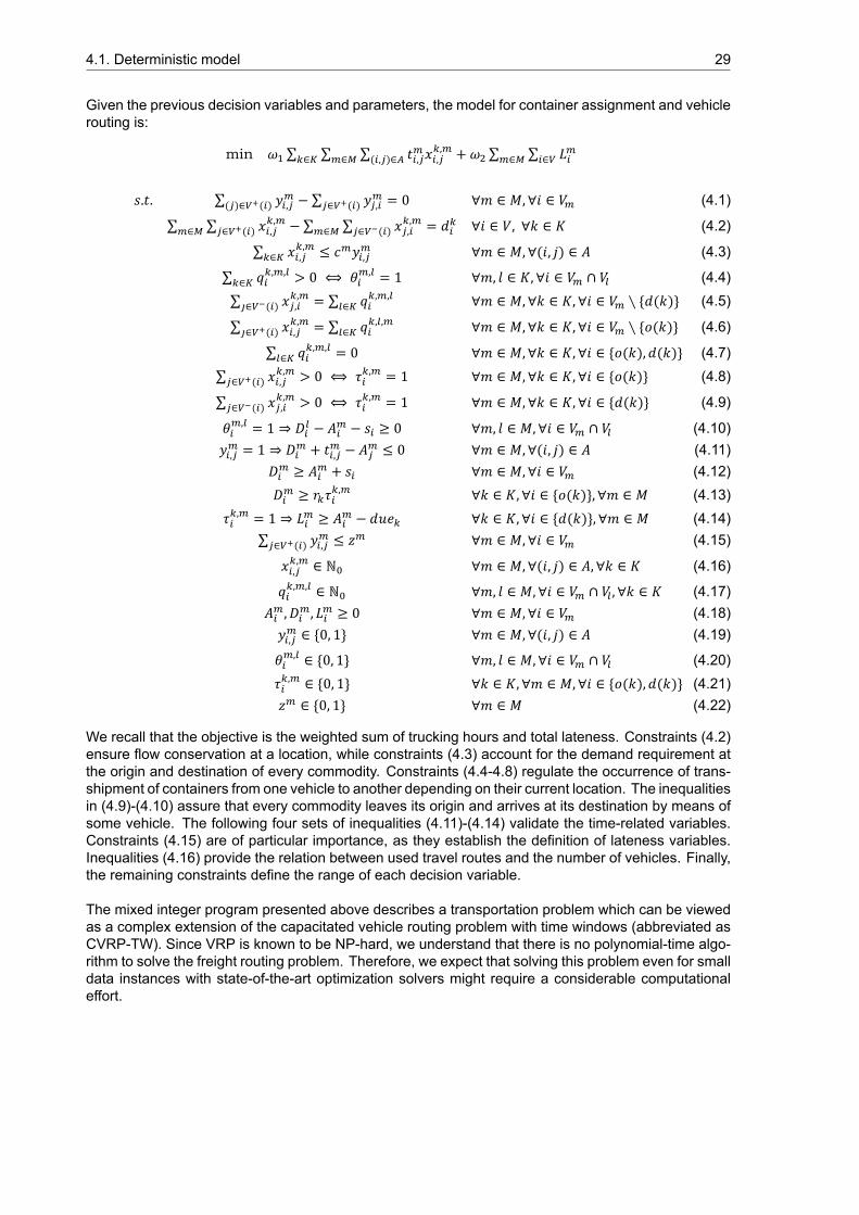
4.1. Deterministic model 29
Given the previous decision variables and parameters, the model for container assignment and vehiclerouting is:
min 𝜔 ∑ ∈ ∑ ∈ ∑( , )∈ 𝑡 , 𝑥 ,, + 𝜔 ∑ ∈ ∑ ∈ 𝐿
𝑠.𝑡. ∑( )∈ ( ) 𝑦 , − ∑ ∈ ( ) 𝑦 , = 0 ∀𝑚 ∈ 𝑀,∀𝑖 ∈ 𝑉 (4.1)
∑ ∈ ∑ ∈ ( ) 𝑥 ,, − ∑ ∈ ∑ ∈ ( ) 𝑥 ,
, = 𝑑 ∀𝑖 ∈ 𝑉, ∀𝑘 ∈ 𝐾 (4.2)
∑ ∈ 𝑥 ,, ≤ 𝑐 𝑦 , ∀𝑚 ∈ 𝑀,∀(𝑖, 𝑗) ∈ 𝐴 (4.3)
∑ ∈ 𝑞 , , > 0 ⟺ 𝜃 , = 1 ∀𝑚, 𝑙 ∈ 𝐾, ∀𝑖 ∈ 𝑉 ∩ 𝑉 (4.4)∑ ∈ ( ) 𝑥 ,
, = ∑ ∈ 𝑞 , , ∀𝑚 ∈ 𝑀,∀𝑘 ∈ 𝐾, ∀𝑖 ∈ 𝑉 ⧵ {𝑑(𝑘)} (4.5)
∑ ∈ ( ) 𝑥 ,, = ∑ ∈ 𝑞 , , ∀𝑚 ∈ 𝑀,∀𝑘 ∈ 𝐾, ∀𝑖 ∈ 𝑉 ⧵ {𝑜(𝑘)} (4.6)
∑ ∈ 𝑞 , , = 0 ∀𝑚 ∈ 𝑀,∀𝑘 ∈ 𝐾, ∀𝑖 ∈ {𝑜(𝑘), 𝑑(𝑘)} (4.7)∑ ∈ ( ) 𝑥 ,
, > 0 ⟺ 𝜏 , = 1 ∀𝑚 ∈ 𝑀,∀𝑘 ∈ 𝐾, ∀𝑖 ∈ {𝑜(𝑘)} (4.8)
∑ ∈ ( ) 𝑥 ,, > 0 ⟺ 𝜏 , = 1 ∀𝑚 ∈ 𝑀,∀𝑘 ∈ 𝐾, ∀𝑖 ∈ {𝑑(𝑘)} (4.9)
𝜃 , = 1 ⇒ 𝐷 − 𝐴 − 𝑠 ≥ 0 ∀𝑚, 𝑙 ∈ 𝑀, ∀𝑖 ∈ 𝑉 ∩ 𝑉 (4.10)𝑦 , = 1 ⇒ 𝐷 + 𝑡 , − 𝐴 ≤ 0 ∀𝑚 ∈ 𝑀,∀(𝑖, 𝑗) ∈ 𝐴 (4.11)
𝐷 ≥ 𝐴 + 𝑠 ∀𝑚 ∈ 𝑀,∀𝑖 ∈ 𝑉 (4.12)𝐷 ≥ 𝑟 𝜏 , ∀𝑘 ∈ 𝐾, ∀𝑖 ∈ {𝑜(𝑘)}, ∀𝑚 ∈ 𝑀 (4.13)
𝜏 , = 1 ⇒ 𝐿 ≥ 𝐴 − 𝑑𝑢𝑒 ∀𝑘 ∈ 𝐾, ∀𝑖 ∈ {𝑑(𝑘)}, ∀𝑚 ∈ 𝑀 (4.14)∑ ∈ ( ) 𝑦 , ≤ 𝑧 ∀𝑚 ∈ 𝑀,∀𝑖 ∈ 𝑉 (4.15)
𝑥 ,, ∈ ℕ ∀𝑚 ∈ 𝑀,∀(𝑖, 𝑗) ∈ 𝐴, ∀𝑘 ∈ 𝐾 (4.16)
𝑞 , , ∈ ℕ ∀𝑚, 𝑙 ∈ 𝑀, ∀𝑖 ∈ 𝑉 ∩ 𝑉, ∀𝑘 ∈ 𝐾 (4.17)𝐴 ,𝐷 , 𝐿 ≥ 0 ∀𝑚 ∈ 𝑀,∀𝑖 ∈ 𝑉 (4.18)𝑦 , ∈ {0, 1} ∀𝑚 ∈ 𝑀, ∀(𝑖, 𝑗) ∈ 𝐴 (4.19)
𝜃 , ∈ {0, 1} ∀𝑚, 𝑙 ∈ 𝑀, ∀𝑖 ∈ 𝑉 ∩ 𝑉 (4.20)𝜏 , ∈ {0, 1} ∀𝑘 ∈ 𝐾, ∀𝑚 ∈ 𝑀, ∀𝑖 ∈ {𝑜(𝑘), 𝑑(𝑘)} (4.21)𝑧 ∈ {0, 1} ∀𝑚 ∈ 𝑀 (4.22)
We recall that the objective is the weighted sum of trucking hours and total lateness. Constraints (4.2)ensure flow conservation at a location, while constraints (4.3) account for the demand requirement atthe origin and destination of every commodity. Constraints (4.4-4.8) regulate the occurrence of trans-shipment of containers from one vehicle to another depending on their current location. The inequalitiesin (4.9)-(4.10) assure that every commodity leaves its origin and arrives at its destination by means ofsome vehicle. The following four sets of inequalities (4.11)-(4.14) validate the time-related variables.Constraints (4.15) are of particular importance, as they establish the definition of lateness variables.Inequalities (4.16) provide the relation between used travel routes and the number of vehicles. Finally,the remaining constraints define the range of each decision variable.
The mixed integer program presented above describes a transportation problem which can be viewedas a complex extension of the capacitated vehicle routing problem with time windows (abbreviated asCVRP-TW). Since VRP is known to be NP-hard, we understand that there is no polynomial-time algo-rithm to solve the freight routing problem. Therefore, we expect that solving this problem even for smalldata instances with state-of-the-art optimization solvers might require a considerable computationaleffort.
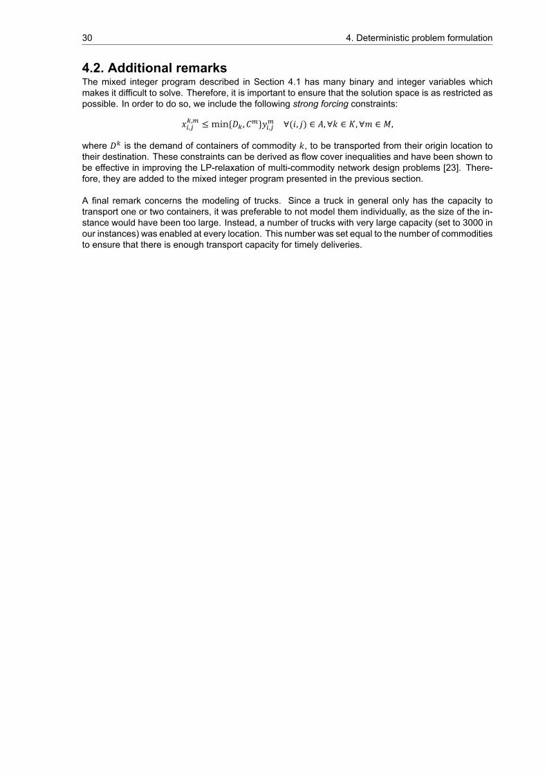
30 4. Deterministic problem formulation
4.2. Additional remarksThe mixed integer program described in Section 4.1 has many binary and integer variables whichmakes it difficult to solve. Therefore, it is important to ensure that the solution space is as restricted aspossible. In order to do so, we include the following strong forcing constraints:
𝑥 ,, ≤min{𝐷 , 𝐶 }𝑦 , ∀(𝑖, 𝑗) ∈ 𝐴, ∀𝑘 ∈ 𝐾, ∀𝑚 ∈ 𝑀,
where 𝐷 is the demand of containers of commodity 𝑘, to be transported from their origin location totheir destination. These constraints can be derived as flow cover inequalities and have been shown tobe effective in improving the LP-relaxation of multi-commodity network design problems [23]. There-fore, they are added to the mixed integer program presented in the previous section.
A final remark concerns the modeling of trucks. Since a truck in general only has the capacity totransport one or two containers, it was preferable to not model them individually, as the size of the in-stance would have been too large. Instead, a number of trucks with very large capacity (set to 3000 inour instances) was enabled at every location. This number was set equal to the number of commoditiesto ensure that there is enough transport capacity for timely deliveries.
5Robust problem formulation
In Chapter 4 we have presented a deterministic model for the freight routing problem which gives opti-mal solutions if the input data is assumed to be fully correct. However, in practice, this is almost neverthe case, as perturbations in data occur due to estimation, prediction or implementation errors. This sortof uncertainty may drastically affect the quality of the solution and it is not considered in deterministicoptimization. Nevertheless, it can be handled by stochastic optimization (SO) and robust optimization(RO). Stochastic programming is a commonly used method which optimizes the problem by makinguse of the parameters’ expected value. This approach generates a number of scenarios that representthe possible realizations of the stochastic parameters, assigns a probability to each of these scenariosand finally, creates a model optimizing over all scenarios. Stochastic programming cannot be usedwhen detailed statistical information is missing or when the number of scenarios becomes too large,making the problem intractable. In [32], it was shown that already for a small instance the freight routingproblem with fixed vehicle routes and stochastic travel times, the scenario tree becomes prohibitivelylarge. Although we will not investigate stochastic programming further, we refer the interested readerto [16].The robust optimization framework on the other hand, is based on obtaining solutions which re-main feasible for any realization of the parameters within a pre-defined uncertainty set. For this reason,we will explore in this chapter how can the adjustable robust optimization be used in order to deal withthe uncertainty in the release times of the containers. In Section 5.1 we present the robust optimizationparadigm and explain how to formulate and solve the robust counterpart. The robust mathematicalformulation of the freight routing problem is given in Section 5.2.
5.1. Robust optimization paradigmRobust optimization is an increasingly popular methodology to model mathematical optimization pro-grams with uncertain data. Instead of assuming a known probability distribution, the uncertain data ispresumed to reside in a user-specified set of realizations, called the uncertainty set. We consider ageneral formulation of an uncertain linear optimization problem:
min{𝑐 𝑥 ∶ 𝐴𝑥 ≤ 𝑏}, (P )
where 𝑐 ∈ ℝ , 𝐴 ∈ ℝ × and 𝑏 ∈ ℝ . Suppose that the matrix 𝐴 is uncertain and it belongs to abounded uncertainty set 𝒰 ⊂ ℝ × . In a similar fashion we assume that right hand side vector 𝑏belongs to uncertainty set 𝒰 ⊂ ℝ , whilst the objective coefficients 𝑐 reside in the uncertainty set𝒰 ⊂ ℝ . The sets 𝒰 , 𝒰 and 𝒰 specify all possible realizations of the uncertain data and arecollectively referred to as the uncertainty set 𝒰. The robust optimization paradigm as described byBen-Tal et al. [14] relies on the following assumptions:
A.1 All decision variables 𝑥 ∈ ℝ represent here-and-now decisions: they should be assigned specificnumerical values as a result of solving the problem before the actual data ‘reveals itself’.
A.2 The decision maker is fully responsible for consequences of the decisions to be made when, andonly when, the actual data is within the prespecified uncertainty set 𝒰.
31
32 5. Robust problem formulation
A.3 All the constraints of the uncertain problem in case are ‘hard’: we cannot tolerate violations ofconstraints when the data is in the uncertainty set 𝒰.
These assumptions indicate what are the relevant feasible solutions of the linear uncertain problemP . The first assumption A.1 asserts that the solution vector should have fixed values or otherwisesaid, it should not contain any components to which there has not been assigned a numerical value.By assumptions A.2 and A.3 this solution vector should satisfy all the constraints, regardless of therealization of the data in the uncertainty set 𝒰. Such a solution is called robust feasible [14]. Thuswe understand that robust optimization is concerned with finding robust feasible solutions for problemswith a predefined uncertainty set.
5.1.1. The robust counterpartWe observe that the linear uncertain problem P exhibits uncertainty in all parameters. In fact, one canshow that this problem can be reformulated in such a way that only the matrix 𝐴 will contain uncertainentries. Firstly, the uncertainty in the objective function can be removed by introducing an additionalcontinuous decision variable 𝑡 ∈ ℝ. Problem P is then equivalent to:
min,{𝑡 ∶ 𝑐 𝑥 − 𝑡 ≤ 0 ∀𝑐 ∈ 𝒰 , 𝐴𝑥 ≤ 𝑏 ∀𝐴 ∈ 𝒰 , ∀𝑏 ∈ 𝒰 }.
Secondly, the uncertain components of vector 𝑏 can be transferred to the matrix 𝐴 in the following way:vector 𝑏 is added as a column of 𝐴 and value 𝑥 = −1 is added as an extra component to the vector𝑥. Then the problem P can be written as:
min,{𝑡 ∶ 𝑐 𝑥 − 𝑡 ≤ 0 ∀𝑐 ∈ 𝒰 , 𝐴𝑥 ≤ 0 ∀𝐴 ∈ 𝒰 ∪ 𝒰 },
Given these two reformulations, we conclude that it is always safe to assume that uncertain quantitiesoccur only in the matrix of coefficients. This being said, we can finally give a most general form of theuncertain linear problem as:
min{𝑐 𝑥 ∶ 𝐴𝑥 ≤ 𝑏 ∀𝐴 ∈ 𝒰} (P)
The robust reformulation of problem P is referred to as the robust counterpart (RC) problem [14] andwe will present it as given in [55]. We assume that the coefficient matrix 𝐴(𝜁) is an affine1 function ofthe uncertain parameter 𝜁:
min{𝑐 𝑥 ∶ 𝐴(𝜁)𝑥 ≤ 𝑏 ∀𝜁 ∈ 𝒵}, (RC)
where 𝒵 ⊂ ℝ denotes the user defined uncertainty set. Recall that a solution 𝑥 is robust feasible if theconstraints 𝐴(𝜁)𝑥 ≤ 𝑏 are satisfied for every value of 𝜁 ∈ 𝒵. As discussed in [14], the robust counterpartof an uncertain linear optimization problem with a certain objective is a ‘constraint-wise’ construction. Inother words, the original 𝑖th row constraint (𝐴𝑥) ≤ 𝑏 ⇔ 𝑎 𝑥 ≤ 𝑏 , (with 𝑎 being the 𝑖th row in 𝐴) fromthe nominal problem is replaced by 𝑎 𝑥 ≤ 𝑏 ∀[𝑎 ; 𝑏 ] ∈ 𝒰 , where 𝒰 is the projection of 𝒰 on thespace of data of 𝑖th constraint: 𝒰 = {[𝑎 ; 𝑏 ] ∶ [𝐴, 𝑏] ∈ 𝒰}. Therefore, we can address the uncertaintyby a single constraint. For instance, we extract one constraint from the robust counterpart problem RCmodeled as an affine expression in terms of 𝜁:
(𝑎 + 𝑃𝜁) 𝑥 ≤ 𝑏 ∀𝜁 ∈ 𝒵, (5.1)
where 𝑎 ∈ ℝ is interpreted as the nominal value of the data, 𝑃 ∈ ℝ × and 𝑏 ∈ ℝ. The idea behindthis process is to reformulate the robust counter part constraint-wise in such a way that it becomescomputationally tractable. The expression in (5.1) has infinitely many constraints due to the for all (∀)quantifier and it is thus intractable in general. In [55] the authors provide a compact overview of thesteps to be followed in order to remove this quantifier. We will closely follow their approach. Considera polyhedral uncertainty set defined as:
𝒵 = {𝜁 ∶ 𝐷𝜁 + 𝑞 ≥ 0}, (5.2)
where 𝐷 ∈ ℝ × , 𝜁 ∈ ℝ and 𝑞 ∈ ℝ .1A function ∶ → is affine if and only if the mapping ↦ ( ) ( ) is linear.
5.1. Robust optimization paradigm 33
In a worst case reformulation, when the realization of the uncertain data yields the largest objectivevalue, one can re-write the nominal problem P as:
𝑎 𝑥 +max{(𝑃 𝑥) 𝜁 ∶ 𝐷𝜁 + 𝑞 ≥ 0} ≤ 𝑏 . (5.3)
By strong duality, the inner maximization problem in the expression above can be replaced by its dual.Therefore, expression (5.3) is equivalent to:
𝑎 𝑥 +min{𝑞 𝑤 ∶ 𝐷 𝑤 = −𝑃 𝑥, 𝑤 ≥ 0} ≤ 𝑏 . (5.4)
We see that in order to satisfy inequality (5.4), it suffices to find at least one 𝑤. Hence, the finalformulation of the RC is given by:
∃𝑤 ∶ 𝑎 𝑥 + 𝑞 𝑥 ≤ 𝑏 , 𝐷 𝑤 = −𝑃 𝑥, 𝑤 ≥ 0, (5.5)
which is an LP feasibility problem.From everything that we have done so far, we conclude that solving the robust counterpart of a generallinear optimization problem with continuous variables and a polyhedral uncertainty set reduces to find-ing a feasible solution to the linear problem described in (5.5). Therefore, the robust counterpart of anuncertain linear program (LP) with a polyhedral uncertainty set is in fact a computationally tractable LP.Moreover, this property also holds for the so-called box uncertainty set of the form: 𝒵 = {𝜁 ∶ ‖𝜁‖ ≤ 1},since the robust counter part in this case is simply given by 𝑎 𝑥 + ‖𝑃 𝑥‖ ≤ 𝑏 [55]. For a thoroughmathematical discussion on tractability properties of the robust counterpart for various uncertainty sets,the reader is referred to the book of Ben-Tal et al. [14].
5.1.2. Adjustable robust optimizationThe robust optimization formulation given in Section 5.1.1 is static in the sense that the numerical valuesof all decision variables must be determined before the uncertain quantities reveal their true value. Forthis reason, the solutions obtained by solving the robust counterpart are indeed robust feasible butsometimes very conservative: they are only optimal for the worst case realizations of the uncertain data.With this static approach it may often be the case that the objective function of the solution becomesunnecessarily high given the actual data realizations attained in practice. This concept is also knownas the price of robustness, described by Bertsimas and Sim [15] as the trade-off between the optimalsolution and robustness. In order to achieve a reasonable price of robustness, the adjustable robustoptimization framework has been proposed [13]. In this framework, assumption A.1 from the robustoptimization paradigm is relaxed, meaning that we allow for some wait-and-see decision variables. Inother words, some decision variables can be adjusted at a later point in time according to the realizationof the data. Most commonly, these adjustable decisions are modeled as functions of the uncertain data.In view of this, the adjustable robust counterpart (ARC) can be formulated as:
min, (⋅){𝑐 𝑥 ∶ 𝐴(𝜁)𝑥 + 𝐵𝑦(𝜁) ≤ 𝑏} ∀𝜁 ∈ 𝒵, (ARC)
where 𝑥 ∈ ℝ represents a first-stage here-and-now decision vector that is made before 𝜁 ∈ ℝ isrealized, 𝑦 ∈ ℝ denotes the second-stage wait-and-see decision vector that can be computed accord-ing to the realization of 𝜁, and 𝐵 ∈ ℝ × is a given coefficient matrix. For the scope of this thesis it issufficient to assume that the matrix 𝐵 does not contain any uncertain elements. In general, it is difficultto optimize over functions, so a commonly used approach is to express the the adjustable decisionvariables as affine functions of the uncertain data namely:
𝑦(𝜁) = 𝑦 + 𝑄𝜁. (5.6)
In the expression above, 𝑦 ∈ ℝ and 𝑄 ∈ ℝ × are here-and-now decisions to be optimized by themodel in the first stage. Substituting the expression for 𝑦 given in equation (5.6) into the ARC we obtainthe affinely adjustable robust counterpart (AARC):
min, ,
{𝑐 𝑥 ∶ 𝐴(𝜁)𝑥 + 𝐵𝑦 + 𝐵𝑄𝜁 ≤ 𝑏 ∀𝜁 ∈ 𝒵}. (AARC)
34 5. Robust problem formulation
Since the AARC is linear in both the decision variables and the uncertain parameter, it can be solved byfollowing the same reformulation steps as in the previous section. Therefore, the AARC has the sametractability as the original robust counter part, regardless of the uncertainty set chosen. Two importantremarks are required here. First of all, the AARC might contain many more decision variables than theRC due to the size of matrix 𝑄. Secondly, although the AARC will likely require more computationaleffort, the solution thus obtained will be at least as good as the one given by solving the RC.
Up to this point, we have presented both the static and the affinely adjustable robust counterpart prob-lems and showed that in the case of linear programs with polyhedral or box uncertainty, both formula-tions are tractable. The fact that we can provide adjustable robust feasible solutions, makes the robustoptimization approach extremely appealing for further applying it to our freight routing problem. Nev-ertheless, as shown in Chapter 4, the model developed includes many binary and integer variablesfor which the mathematical treatment in sections 5.1.1 and 5.1.2 is not directly applicable. Therefore,we will further discuss how robust optimization techniques can be used in the context of mixed integerprograms.
5.1.3. Robust optimization for mixed integer programsA mixed integer program is a mathematical program which contains both real valued decision variablesand variables restricted to take integer values. It is well known that determining whether a feasiblesolution of a given mixed integer program with rational coefficients exists is in the class of NP-completeproblems [24]. As such, we expect that a robust counterpart of a mixed integer linear program is alsointractable. Consider the general form of a mixed integer program:
min,{𝑐 𝑥 + 𝑑 𝑦 ∶ 𝐴𝑥 + 𝐺𝑦 ≤ 𝑝, 𝑥 ∈ ℤ , 𝑦 ∈ ℝ }, (MIP)
where 𝑐 ∈ ℚ and 𝑑 ∈ ℚ are given cost vectors, 𝐴 ∈ ℚ × and 𝐺 ∈ ℚ × are coefficients matricesand 𝑝 ∈ ℚ . We assume that the matrix 𝐴 is the only element affected by uncertainty. This assumptionis motivated by our deterministic model in Chapter 4, in which the uncertain release time is multipliedwith a binary variable in constraints (4.14). Thus we consider a model of the form:
min∈ℤ , ∈ℝ
{𝑐 𝑥 + 𝑑 𝑦 ∶ 𝐴(𝜁)𝑥 + 𝐺𝑦 ≤ 𝑝, ∀𝜁 ∈ 𝒵}. (RC-MIP)
Since uncertainty was showed to appear constraint-wise in a general linear program, we can once againmodel uncertainty affected constraints by an affine transformation of the uncertainty term 𝜁 ∈ 𝒵 namely,every element of 𝐴 can be written as a summation between a linear combination of the components ofvector 𝜁 and a constant:
𝐴(𝜁) = [𝑎 (𝜁) 𝑎 (𝜁) … 𝑎 (𝜁)] = [𝑎 𝑎 … 𝑎 ] + [𝑃 𝜁 𝑃 𝜁 … 𝑃 𝜁] . (5.7)
The robust counterpart then contains constraints of the form:
min∈ℤ , ∈ℝ
{𝑐 𝑥 + 𝑑 𝑦 ∶ (𝑎 + 𝑃𝜁) 𝑥 + 𝑔 𝑦 ≤ 𝑝 , ∀𝑖 ∈ 1,… , 𝑙 ∀𝜁 ∈ 𝒵}, (5.8)
where 𝑎 ∈ ℚ is the nominal value, 𝑃 ∈ ℝ × is the matrix with vectors 𝑃 , 𝑃 ,… , 𝑃 ∈ ℝ as columns,𝑔 is a vector corresponding to the 𝑖th row of matrix 𝐺 and 𝑝 is the 𝑖th entry of vector 𝑝. Just as in thecase of a general linear program, we now wish to bring the RC-MIP problem into a reasonable form,removing the ‘for all’ (∀) operator. The uncertainty set to be considered is the simple box uncertainty:
𝒵 = {‖𝜁‖ ≤ 1}. (5.9)
This kind of uncertainty set is the most intuitive for the freight routing problem, since the release timeof a container is assumed to belong to a certain bounded interval of time. Using the worst-case valuesof the uncertain parameter 𝜁, the robust counter part RC-MIP is re-formulated as:
min∈ℤ , ∈ℝ
{𝑐 𝑥 + 𝑑 𝑦 ∶ 𝑎 𝑥 + ‖𝑃 𝑥‖ + 𝑔 𝑦 ≤ 𝑝 ∀𝑖 ∈ 1,… , 𝑙}. (5.10)
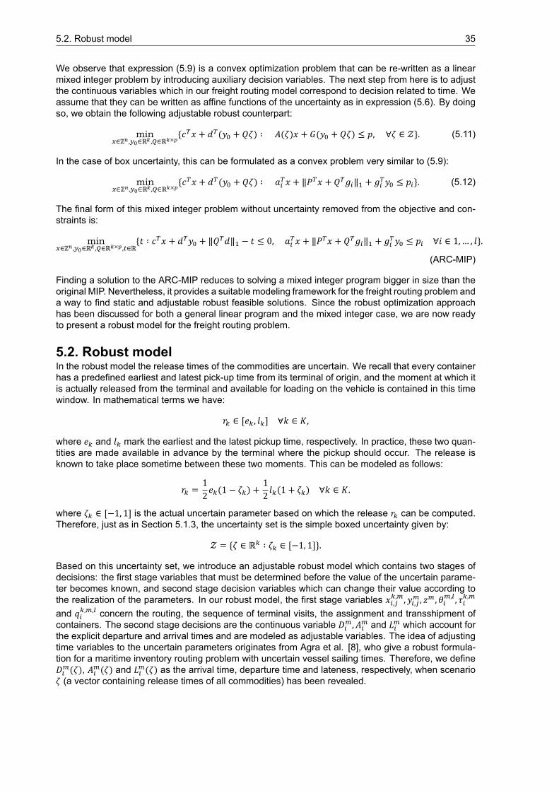
5.2. Robust model 35
We observe that expression (5.9) is a convex optimization problem that can be re-written as a linearmixed integer problem by introducing auxiliary decision variables. The next step from here is to adjustthe continuous variables which in our freight routing model correspond to decision related to time. Weassume that they can be written as affine functions of the uncertainty as in expression (5.6). By doingso, we obtain the following adjustable robust counterpart:
min∈ℤ , ∈ℝ , ∈ℝ × {𝑐 𝑥 + 𝑑 (𝑦 + 𝑄𝜁) ∶ 𝐴(𝜁)𝑥 + 𝐺(𝑦 + 𝑄𝜁) ≤ 𝑝, ∀𝜁 ∈ 𝒵}. (5.11)
In the case of box uncertainty, this can be formulated as a convex problem very similar to (5.9):
min∈ℤ , ∈ℝ , ∈ℝ × {𝑐 𝑥 + 𝑑 (𝑦 + 𝑄𝜁) ∶ 𝑎 𝑥 + ‖𝑃 𝑥 + 𝑄 𝑔 ‖ + 𝑔 𝑦 ≤ 𝑝 }. (5.12)
The final form of this mixed integer problem without uncertainty removed from the objective and con-straints is:
min∈ℤ , ∈ℝ , ∈ℝ × , ∈ℝ
{𝑡 ∶ 𝑐 𝑥 + 𝑑 𝑦 + ‖𝑄 𝑑‖ − 𝑡 ≤ 0, 𝑎 𝑥 + ‖𝑃 𝑥 + 𝑄 𝑔 ‖ + 𝑔 𝑦 ≤ 𝑝 ∀𝑖 ∈ 1,… , 𝑙}.
(ARC-MIP)
Finding a solution to the ARC-MIP reduces to solving a mixed integer program bigger in size than theoriginal MIP. Nevertheless, it provides a suitable modeling framework for the freight routing problem anda way to find static and adjustable robust feasible solutions. Since the robust optimization approachhas been discussed for both a general linear program and the mixed integer case, we are now readyto present a robust model for the freight routing problem.
5.2. Robust modelIn the robust model the release times of the commodities are uncertain. We recall that every containerhas a predefined earliest and latest pick-up time from its terminal of origin, and the moment at which itis actually released from the terminal and available for loading on the vehicle is contained in this timewindow. In mathematical terms we have:
𝑟 ∈ [𝑒 , 𝑙 ] ∀𝑘 ∈ 𝐾,
where 𝑒 and 𝑙 mark the earliest and the latest pickup time, respectively. In practice, these two quan-tities are made available in advance by the terminal where the pickup should occur. The release isknown to take place sometime between these two moments. This can be modeled as follows:
𝑟 = 12𝑒 (1 − 𝜁 ) +
12𝑙 (1 + 𝜁 ) ∀𝑘 ∈ 𝐾.
where 𝜁 ∈ [−1, 1] is the actual uncertain parameter based on which the release 𝑟 can be computed.Therefore, just as in Section 5.1.3, the uncertainty set is the simple boxed uncertainty given by:
𝒵 = {𝜁 ∈ ℝ ∶ 𝜁 ∈ [−1, 1]}.
Based on this uncertainty set, we introduce an adjustable robust model which contains two stages ofdecisions: the first stage variables that must be determined before the value of the uncertain parame-ter becomes known, and second stage decision variables which can change their value according tothe realization of the parameters. In our robust model, the first stage variables 𝑥 ,
, , 𝑦 , , 𝑧 , 𝜃 , , 𝜏 ,
and 𝑞 , , concern the routing, the sequence of terminal visits, the assignment and transshipment ofcontainers. The second stage decisions are the continuous variable 𝐷 , 𝐴 and 𝐿 which account forthe explicit departure and arrival times and are modeled as adjustable variables. The idea of adjustingtime variables to the uncertain parameters originates from Agra et al. [8], who give a robust formula-tion for a maritime inventory routing problem with uncertain vessel sailing times. Therefore, we define𝐷 (𝜁), 𝐴 (𝜁) and 𝐿 (𝜁) as the arrival time, departure time and lateness, respectively, when scenario𝜁 (a vector containing release times of all commodities) has been revealed.
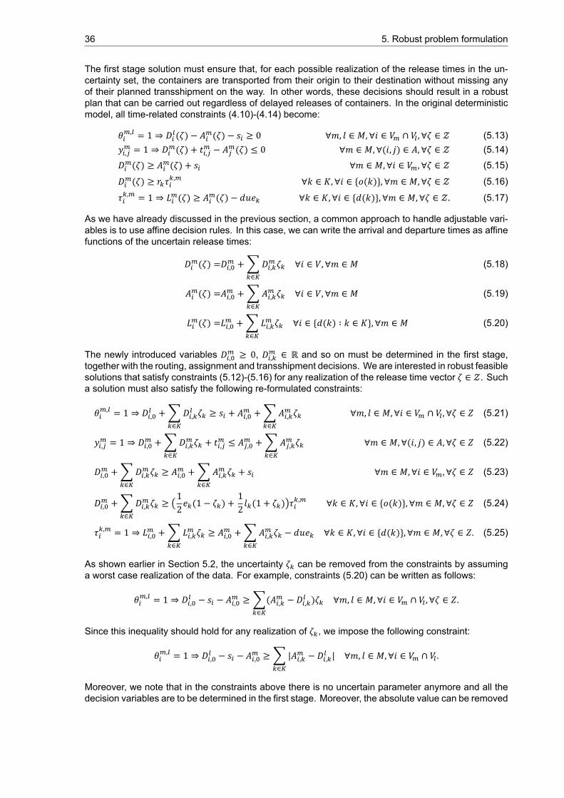
36 5. Robust problem formulation
The first stage solution must ensure that, for each possible realization of the release times in the un-certainty set, the containers are transported from their origin to their destination without missing anyof their planned transshipment on the way. In other words, these decisions should result in a robustplan that can be carried out regardless of delayed releases of containers. In the original deterministicmodel, all time-related constraints (4.10)-(4.14) become:
𝜃 , = 1 ⇒ 𝐷 (𝜁) − 𝐴 (𝜁) − 𝑠 ≥ 0 ∀𝑚, 𝑙 ∈ 𝑀, ∀𝑖 ∈ 𝑉 ∩ 𝑉, ∀𝜁 ∈ 𝒵 (5.13)𝑦 , = 1 ⇒ 𝐷 (𝜁) + 𝑡 , − 𝐴 (𝜁) ≤ 0 ∀𝑚 ∈ 𝑀,∀(𝑖, 𝑗) ∈ 𝐴, ∀𝜁 ∈ 𝒵 (5.14)𝐷 (𝜁) ≥ 𝐴 (𝜁) + 𝑠 ∀𝑚 ∈ 𝑀,∀𝑖 ∈ 𝑉 , ∀𝜁 ∈ 𝒵 (5.15)
𝐷 (𝜁) ≥ 𝑟 𝜏 , ∀𝑘 ∈ 𝐾, ∀𝑖 ∈ {𝑜(𝑘)}, ∀𝑚 ∈ 𝑀, ∀𝜁 ∈ 𝒵 (5.16)
𝜏 , = 1 ⇒ 𝐿 (𝜁) ≥ 𝐴 (𝜁) − 𝑑𝑢𝑒 ∀𝑘 ∈ 𝐾, ∀𝑖 ∈ {𝑑(𝑘)}, ∀𝑚 ∈ 𝑀, ∀𝜁 ∈ 𝒵. (5.17)
As we have already discussed in the previous section, a common approach to handle adjustable vari-ables is to use affine decision rules. In this case, we can write the arrival and departure times as affinefunctions of the uncertain release times:
𝐷 (𝜁) =𝐷 , +∑∈𝐷 , 𝜁 ∀𝑖 ∈ 𝑉, ∀𝑚 ∈ 𝑀 (5.18)
𝐴 (𝜁) =𝐴 , +∑∈𝐴 , 𝜁 ∀𝑖 ∈ 𝑉, ∀𝑚 ∈ 𝑀 (5.19)
𝐿 (𝜁) =𝐿 , +∑∈𝐿 , 𝜁 ∀𝑖 ∈ {𝑑(𝑘) ∶ 𝑘 ∈ 𝐾}, ∀𝑚 ∈ 𝑀 (5.20)
The newly introduced variables 𝐷 , ≥ 0, 𝐷 , ∈ ℝ and so on must be determined in the first stage,together with the routing, assignment and transshipment decisions. We are interested in robust feasiblesolutions that satisfy constraints (5.12)-(5.16) for any realization of the release time vector 𝜁 ∈ 𝒵. Sucha solution must also satisfy the following re-formulated constraints:
𝜃 , = 1 ⇒ 𝐷 , +∑∈𝐷 , 𝜁 ≥ 𝑠 + 𝐴 , +∑
∈𝐴 , 𝜁 ∀𝑚, 𝑙 ∈ 𝑀, ∀𝑖 ∈ 𝑉 ∩ 𝑉, ∀𝜁 ∈ 𝑍 (5.21)
𝑦 , = 1 ⇒ 𝐷 , +∑∈𝐷 , 𝜁 + 𝑡 , ≤ 𝐴 , +∑
∈𝐴 , 𝜁 ∀𝑚 ∈ 𝑀,∀(𝑖, 𝑗) ∈ 𝐴, ∀𝜁 ∈ 𝑍 (5.22)
𝐷 , +∑∈𝐷 , 𝜁 ≥ 𝐴 , +∑
∈𝐴 , 𝜁 + 𝑠 ∀𝑚 ∈ 𝑀,∀𝑖 ∈ 𝑉 , ∀𝜁 ∈ 𝑍 (5.23)
𝐷 , +∑∈𝐷 , 𝜁 ≥ (12𝑒 (1 − 𝜁 ) +
12𝑙 (1 + 𝜁 ))𝜏
, ∀𝑘 ∈ 𝐾, ∀𝑖 ∈ {𝑜(𝑘)}, ∀𝑚 ∈ 𝑀, ∀𝜁 ∈ 𝑍 (5.24)
𝜏 , = 1 ⇒ 𝐿 , +∑∈𝐿 , 𝜁 ≥ 𝐴 , +∑
∈𝐴 , 𝜁 − 𝑑𝑢𝑒 ∀𝑘 ∈ 𝐾, ∀𝑖 ∈ {𝑑(𝑘)}, ∀𝑚 ∈ 𝑀, ∀𝜁 ∈ 𝑍. (5.25)
As shown earlier in Section 5.2, the uncertainty 𝜁 can be removed from the constraints by assuminga worst case realization of the data. For example, constraints (5.20) can be written as follows:
𝜃 , = 1 ⇒ 𝐷 , − 𝑠 − 𝐴 , ≥ ∑∈(𝐴 , − 𝐷 , )𝜁 ∀𝑚, 𝑙 ∈ 𝑀, ∀𝑖 ∈ 𝑉 ∩ 𝑉, ∀𝜁 ∈ 𝑍.
Since this inequality should hold for any realization of 𝜁 , we impose the following constraint:
𝜃 , = 1 ⇒ 𝐷 , − 𝑠 − 𝐴 , ≥ ∑∈|𝐴 , − 𝐷 , | ∀𝑚, 𝑙 ∈ 𝑀, ∀𝑖 ∈ 𝑉 ∩ 𝑉.
Moreover, we note that in the constraints above there is no uncertain parameter anymore and all thedecision variables are to be determined in the first stage. Moreover, the absolute value can be removed
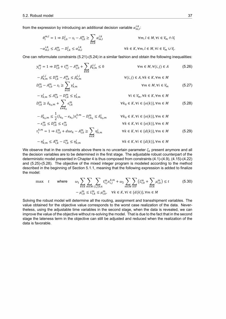
5.2. Robust model 37
from the expression by introducing an additional decision variable 𝛼 ,, :
𝜃 , = 1 ⇒ 𝐷 , − 𝑠 − 𝐴 , ≥ ∑∈𝛼 ,
, ∀𝑚, 𝑙 ∈ 𝑀, ∀𝑖 ∈ 𝑉 ∩ 𝑉
−𝛼 ,, ≤ 𝐴 , − 𝐷 , ≤ 𝛼 ,
, ∀𝑘 ∈ 𝐾, ∀𝑚, 𝑙 ∈ 𝑀, ∀𝑖 ∈ 𝑉 ∪ 𝑉.
One can reformulate constraints (5.21)-(5.24) in a similar fashion and obtain the following inequalities:
𝑦 , = 1 ⇒ 𝐷 , + 𝑡 , − 𝐴 , +∑∈𝛽 ,, ≤ 0 ∀𝑚 ∈ 𝑀,∀(𝑖, 𝑗) ∈ 𝐴 (5.26)
− 𝛽 ,, ≤ 𝐷 , − 𝐴 , ≤ 𝛽
,, ∀(𝑖, 𝑗) ∈ 𝐴, ∀𝑘 ∈ 𝐾, ∀𝑚 ∈ 𝑀
𝐷 , − 𝐴 , − 𝑠 ≥ ∑∈𝛾 , ∀𝑚 ∈ 𝑀,∀𝑖 ∈ 𝑉 (5.27)
− 𝛾 , ≤ 𝐴 , − 𝐷 , ≤ 𝛾 , ∀𝑖 ∈ 𝑉 , ∀𝑘 ∈ 𝐾, ∀𝑚 ∈ 𝑀
𝐷 , ≥ 𝛿 , + ∑ 𝜖 , ∀𝑘 ∈ 𝐾, ∀𝑖 ∈ {𝑜(𝑘)}, ∀𝑚 ∈ 𝑀 (5.28)
− 𝛿 , ≤ 12(𝑙 − 𝑒 )𝜏 , − 𝐷 , ≤ 𝛿 , ∀𝑘 ∈ 𝐾, ∀𝑖 ∈ {𝑜(𝑘)}, ∀𝑚 ∈ 𝑀
− 𝜖 , ≤ 𝐷 , ≤ 𝜖 , ∀𝑘 ∈ 𝐾, ∀𝑖 ∈ {𝑜(𝑘)}, ∀𝑚 ∈ 𝑀
𝜏 , = 1 ⇒ 𝐿 , + 𝑑𝑢𝑒 − 𝐴 , ≥ ∑∈𝜂 , ∀𝑘 ∈ 𝐾, ∀𝑖 ∈ {𝑑(𝑘)}, ∀𝑚 ∈ 𝑀 (5.29)
− 𝜂 , ≤ 𝐴 , − 𝐿 , ≤ 𝜂 , ∀𝑘 ∈ 𝐾, ∀𝑖 ∈ {𝑑(𝑘)}, ∀𝑚 ∈ 𝑀
We observe that in the constraints above there is no uncertain parameter 𝜁 present anymore and allthe decision variables are to be determined in the first stage. The adjustable robust counterpart of thedeterministic model presented in Chapter 4 is thus composed from constraints (4.1)-(4.9), (4.15)-(4.22)and (5.25)-(5.28). The objective of the mixed integer program is modeled according to the methoddescribed in the beginning of Section 5.1.1, meaning that the following expression is added to finalizethe model:
max 𝑡 where 𝜔 ∑∈∑∈
∑( , )∈
𝑡 , 𝑥 ,, + 𝜔 ∑
∈∑∈(𝐿 , +∑
∈𝜇 , ) ≤ 𝑡 (5.30)
− 𝜇 , ≤ 𝐿 , ≤ 𝜇 , , ∀𝑘 ∈ 𝐾, ∀𝑖 ∈ {𝑑(𝑘)}, ∀𝑚 ∈ 𝑀
Solving the robust model will determine all the routing, assignment and transshipment variables. Thevalue obtained for the objective value corresponds to the worst case realization of the data. Never-theless, using the adjustable time variables in the second stage, when the data is revealed, we canimprove the value of the objective without re-solving the model. That is due to the fact that in the secondstage the lateness term in the objective can still be adjusted and reduced when the realization of thedata is favorable.

6Computational results
In this chapter, we report on the solutions found for the deterministic and robust formulations of thefreight routing problem and compare them to past approaches. In Section 6.1. it is explained how thetest instances were generated. Section 6.2 contains the results for the deterministic model, whilst thefindings for the robust approach are shown in Section 6.3. All results are interpreted and discussed inSection 6.4.
6.1. Instance generationIn order to test the models that were given in chapters 4 and 5, we generated multiple instances. Thesewere inspired from the work of Kishan Kalicharan [34], a project colleague from TNO who has designeda transport network of eight terminal locations based on Google Maps data. Since some of these loca-tions represented clustered terminals, the original instances were modified to include only nodes whichcorrespond to actual physical locations in real life. For comparison purposes, the number of locationswas kept the same. The barge travel times on waterways were assumed to be fixed and their valueswere approximated using online tools which compute sea distances based on the speed of the vessel.In our transport infrastructure, we assume that some of the locations are terminals, where containerscan be transshiped, and some of them are customers, serving as end-locations for the containers.There is also direct connection between every pait of locations in our model. Furthermore, we assumethat the service time is the same at every location. There is a set of commodities (bookings with one ormore containers) that need to be transported from the terminals to the customer locations. As in [34],the demand value of each commodity is randomly chosen in the interval [0, 125].
Barges and trucks are available for container transport. The capacity of barges is assumed to beof 100 containers. These barges always start at a particular terminal which in real-life interpretation ina hub-location. We assume that there is an infinite amount of trucks of large capacity available at everylocation. To ensure that all containers can be transported, the total capacity of all vehicles is alwayslarger than the total demand of all commodities [41]. Finally, the due dates and release times of thecontainers are chosen in such a way that the difference between them is strictly larger than the timerequired by barge to travel on the direct connection arc from the origin of the containers to the theirdestination.
To assess the computational difficulty of our models we create instances with 8 nodes, 6 and 12 barges,and 5, 10, 20 and 30 commodities. In total, we generate 10 instances which are tested for three differ-ent objective functions by varying the values of the weights 𝜔 and 𝜔 . We denote a problem instanceby 𝑘𝑚, where 𝑘 the number of commodities and 𝑚 the number of available barges. Both the deter-ministic and the robust model were implemented in AIMMS Developer version 4.53, a mathematicaloptimization modeling tool, and solved with CPLEX optimization solver (Version 12.8, 32-bit). Numeri-cal experiments were carried out on a DELL Latitude E7240 laptop with an Intel(R) Core(TM) i5-4310UCPU 2.00 GHz 2.60 GHz processor and 8 GB RAM memory. This laptop is operational on a 64-bitoperating system.
39
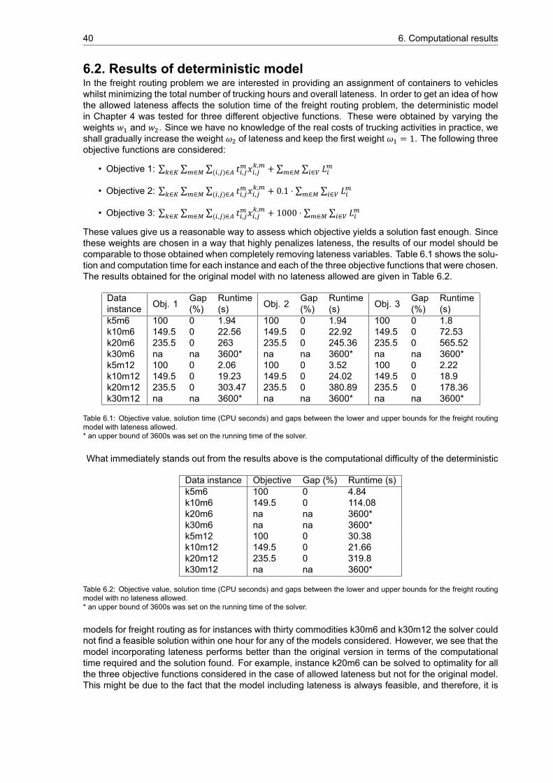
40 6. Computational results
6.2. Results of deterministic modelIn the freight routing problem we are interested in providing an assignment of containers to vehicleswhilst minimizing the total number of trucking hours and overall lateness. In order to get an idea of howthe allowed lateness affects the solution time of the freight routing problem, the deterministic modelin Chapter 4 was tested for three different objective functions. These were obtained by varying theweights 𝑤 and 𝑤 . Since we have no knowledge of the real costs of trucking activities in practice, weshall gradually increase the weight 𝜔 of lateness and keep the first weight 𝜔 = 1. The following threeobjective functions are considered:
• Objective 1: ∑ ∈ ∑ ∈ ∑( , )∈ 𝑡 , 𝑥 ,, + ∑ ∈ ∑ ∈ 𝐿
• Objective 2: ∑ ∈ ∑ ∈ ∑( , )∈ 𝑡 , 𝑥 ,, + 0.1 ⋅ ∑ ∈ ∑ ∈ 𝐿
• Objective 3: ∑ ∈ ∑ ∈ ∑( , )∈ 𝑡 , 𝑥 ,, + 1000 ⋅ ∑ ∈ ∑ ∈ 𝐿
These values give us a reasonable way to assess which objective yields a solution fast enough. Sincethese weights are chosen in a way that highly penalizes lateness, the results of our model should becomparable to those obtained when completely removing lateness variables. Table 6.1 shows the solu-tion and computation time for each instance and each of the three objective functions that were chosen.The results obtained for the original model with no lateness allowed are given in Table 6.2.
Datainstance Obj. 1 Gap
(%)Runtime(s) Obj. 2 Gap
(%)Runtime(s) Obj. 3 Gap
(%)Runtime(s)
k5m6 100 0 1.94 100 0 1.94 100 0 1.8k10m6 149.5 0 22.56 149.5 0 22.92 149.5 0 72.53k20m6 235.5 0 263 235.5 0 245.36 235.5 0 565.52k30m6 na na 3600* na na 3600* na na 3600*k5m12 100 0 2.06 100 0 3.52 100 0 2.22k10m12 149.5 0 19.23 149.5 0 24.02 149.5 0 18.9k20m12 235.5 0 303.47 235.5 0 380.89 235.5 0 178.36k30m12 na na 3600* na na 3600* na na 3600*
Table 6.1: Objective value, solution time (CPU seconds) and gaps between the lower and upper bounds for the freight routingmodel with lateness allowed.* an upper bound of 3600s was set on the running time of the solver.
What immediately stands out from the results above is the computational difficulty of the deterministic
Data instance Objective Gap (%) Runtime (s)k5m6 100 0 4.84k10m6 149.5 0 114.08k20m6 na na 3600*k30m6 na na 3600*k5m12 100 0 30.38k10m12 149.5 0 21.66k20m12 235.5 0 319.8k30m12 na na 3600*
Table 6.2: Objective value, solution time (CPU seconds) and gaps between the lower and upper bounds for the freight routingmodel with no lateness allowed.* an upper bound of 3600s was set on the running time of the solver.
models for freight routing as for instances with thirty commodities k30m6 and k30m12 the solver couldnot find a feasible solution within one hour for any of the models considered. However, we see that themodel incorporating lateness performs better than the original version in terms of the computationaltime required and the solution found. For example, instance k20m6 can be solved to optimality for allthe three objective functions considered in the case of allowed lateness but not for the original model.This might be due to the fact that the model including lateness is always feasible, and therefore, it is
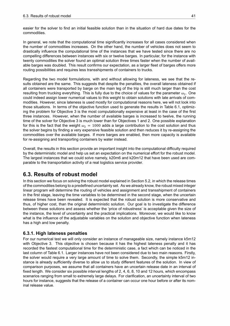
6.3. Results of robust model 41
easier for the solver to find an initial feasible solution than in the situation of hard due dates for thecommodities.
In general, we note that the computational time significantly increases for all cases considered whenthe number of commodities increases. On the other hand, the number of vehicles does not seem todrastically influence the computational time of the instances that we have tested since there are nocompelling differences between instances with six or twelve barges. In particular, for the instance withtwenty commodities the solver found an optimal solution three times faster when the number of avail-able barges was doubled. This result confirms our expectation, as a larger fleet of barges offers morerouting possibilities and requires less transshipments of containers to trucks.
Regarding the two model formulations, with and without allowing for lateness, we see that the re-sults obtained are the same. This suggests that despite the penalties, the overall lateness obtained ifall containers were transported by barge on the main leg of the trip is still much larger than the costresulting from trucking everything. This is fully due to the choice of values for the parameter 𝜔 . Onecould indeed assign lower numerical values to this weight to obtain solutions with late arrivals of com-modities. However, since lateness is used mostly for computational reasons here, we will not look intothose situations. In terms of the objective function used to generate the results in Table 6.1, optimiz-ing the problem for Objective 3 is the most computationally expensive at least in the case of the firstthree instances. However, when the number of available barges is increased to twelve, the runningtime of the solver for Objective 3 is much lower than for Objectives 1 and 2. One possible explanationfor this is the fact that the weight 𝜔 = 1000 adds a large contribution to the cost solution and thusthe solver begins by finding a very expensive feasible solution and then reduces it by re-assigning thecommodities over the available barges. If more barges are enabled, then more capacity is availablefor re-assigning and transporting containers by water instead.
Overall, the results in this section provide an important insight into the computational difficulty requiredby the deterministic model and help us set an expectation on the numerical effort for the robust model.The largest instances that we could solve namely, k20m6 and k20m12 that have been used are com-parable to the transportation activity of a real logistics service provider.
6.3. Results of robust modelIn this section we focus on solving the robust model explained in Section 5.2, in which the release timesof the commodities belong to a predefined uncertainty set. As we already know, the robust mixed integerlinear program will determine the routing of vehicles and assignment and transshipment of containersin the first stage, leaving the time variables to be determined in the second stage, when the uncertainrelease times have been revealed. It is expected that the robust solution is more conservative andthus, of higher cost, than the original deterministic solution. Our goal is to investigate the differencebetween these solutions and assess whether the ‘price of robustness’ is acceptable given the size ofthe instance, the level of uncertainty and the practical implications. Moreover, we would like to knowwhat is the influence of the adjustable variables on the solution and objective function when latenesshas a high and low penalty.
6.3.1. High lateness penaltiesFor our numerical test we will only consider an instance of manageable size, namely instance k5m12with Objective 3. This objective is chosen because it has the highest lateness penalty and it hasrecorded the fastest computational time for the deterministic case, a fact which can be noticed in thelast column of Table 6.1. Larger instances have not been considered due to two main reasons. Firstly,the solver would require a very large amount of time to solve them. Secondly, the simple k5m12 in-stance is already sufficiently diverse to allow us to study different features of the solution. In view ofcomparison purposes, we assume that all containers have an uncertain release date in an interval offixed length. We consider six possible interval lengths of 2, 4, 6, 8, 10 and 12 hours, which encompassscenarios ranging from small to extremely large delays. For clarification, an uncertainty interval of twohours for instance, suggests that the release of a container can occur one hour before or after its nom-inal release value.
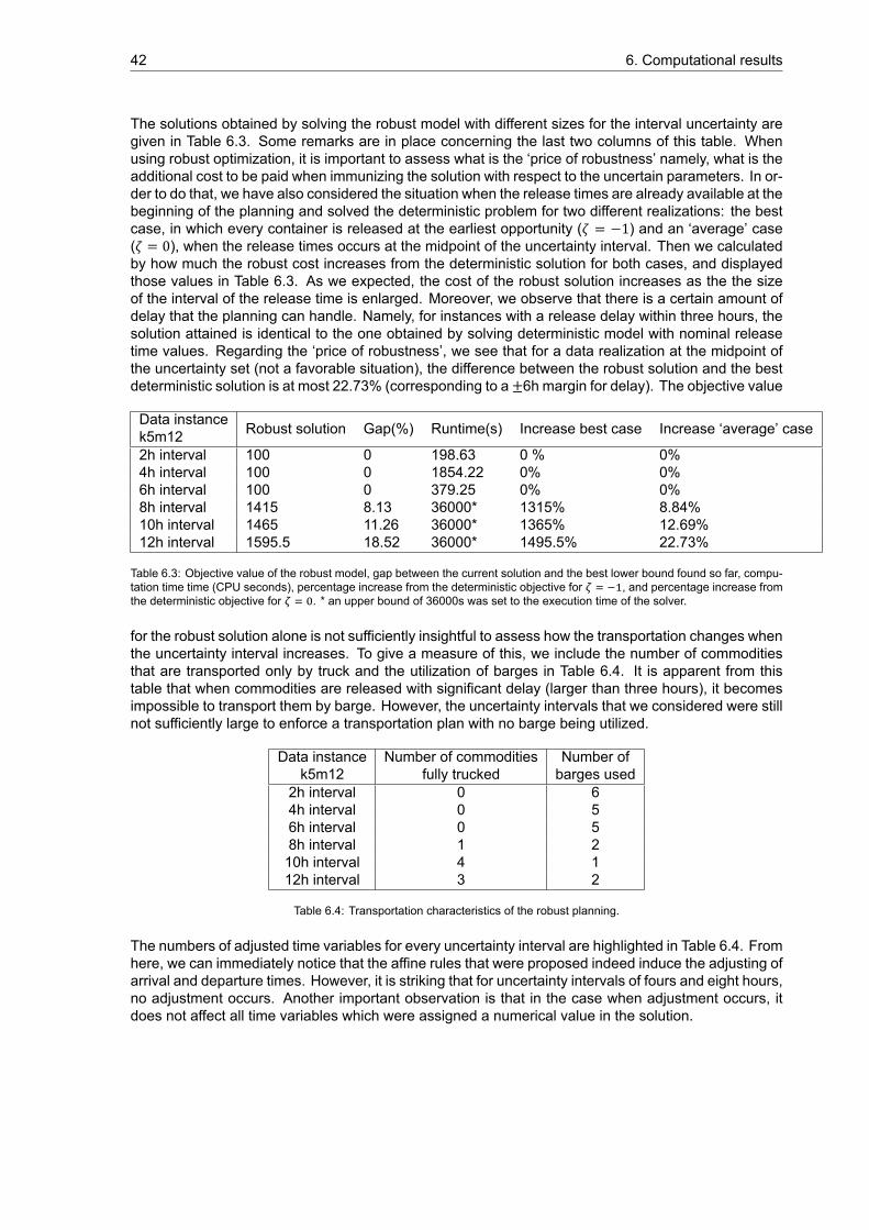
42 6. Computational results
The solutions obtained by solving the robust model with different sizes for the interval uncertainty aregiven in Table 6.3. Some remarks are in place concerning the last two columns of this table. Whenusing robust optimization, it is important to assess what is the ‘price of robustness’ namely, what is theadditional cost to be paid when immunizing the solution with respect to the uncertain parameters. In or-der to do that, we have also considered the situation when the release times are already available at thebeginning of the planning and solved the deterministic problem for two different realizations: the bestcase, in which every container is released at the earliest opportunity (𝜁 = −1) and an ‘average’ case(𝜁 = 0), when the release times occurs at the midpoint of the uncertainty interval. Then we calculatedby how much the robust cost increases from the deterministic solution for both cases, and displayedthose values in Table 6.3. As we expected, the cost of the robust solution increases as the the sizeof the interval of the release time is enlarged. Moreover, we observe that there is a certain amount ofdelay that the planning can handle. Namely, for instances with a release delay within three hours, thesolution attained is identical to the one obtained by solving deterministic model with nominal releasetime values. Regarding the ‘price of robustness’, we see that for a data realization at the midpoint ofthe uncertainty set (not a favorable situation), the difference between the robust solution and the bestdeterministic solution is at most 22.73% (corresponding to a ±6h margin for delay). The objective value
Data instancek5m12 Robust solution Gap(%) Runtime(s) Increase best case Increase ‘average’ case
2h interval 100 0 198.63 0 % 0%4h interval 100 0 1854.22 0% 0%6h interval 100 0 379.25 0% 0%8h interval 1415 8.13 36000* 1315% 8.84%10h interval 1465 11.26 36000* 1365% 12.69%12h interval 1595.5 18.52 36000* 1495.5% 22.73%
Table 6.3: Objective value of the robust model, gap between the current solution and the best lower bound found so far, compu-tation time time (CPU seconds), percentage increase from the deterministic objective for , and percentage increase fromthe deterministic objective for . * an upper bound of 36000s was set to the execution time of the solver.
for the robust solution alone is not sufficiently insightful to assess how the transportation changes whenthe uncertainty interval increases. To give a measure of this, we include the number of commoditiesthat are transported only by truck and the utilization of barges in Table 6.4. It is apparent from thistable that when commodities are released with significant delay (larger than three hours), it becomesimpossible to transport them by barge. However, the uncertainty intervals that we considered were stillnot sufficiently large to enforce a transportation plan with no barge being utilized.
Data instancek5m12
Number of commoditiesfully trucked
Number ofbarges used
2h interval 0 64h interval 0 56h interval 0 58h interval 1 210h interval 4 112h interval 3 2
Table 6.4: Transportation characteristics of the robust planning.
The numbers of adjusted time variables for every uncertainty interval are highlighted in Table 6.4. Fromhere, we can immediately notice that the affine rules that were proposed indeed induce the adjusting ofarrival and departure times. However, it is striking that for uncertainty intervals of fours and eight hours,no adjustment occurs. Another important observation is that in the case when adjustment occurs, itdoes not affect all time variables which were assigned a numerical value in the solution.
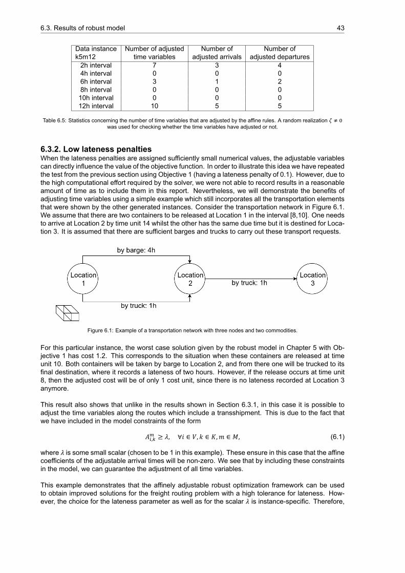
6.3. Results of robust model 43
Data instancek5m12
Number of adjustedtime variables
Number ofadjusted arrivals
Number ofadjusted departures
2h interval 7 3 44h interval 0 0 06h interval 3 1 28h interval 0 0 010h interval 0 0 012h interval 10 5 5
Table 6.5: Statistics concerning the number of time variables that are adjusted by the affine rules. A random realizationwas used for checking whether the time variables have adjusted or not.
6.3.2. Low lateness penaltiesWhen the lateness penalties are assigned sufficiently small numerical values, the adjustable variablescan directly influence the value of the objective function. In order to illustrate this idea we have repeatedthe test from the previous section using Objective 1 (having a lateness penalty of 0.1). However, due tothe high computational effort required by the solver, we were not able to record results in a reasonableamount of time as to include them in this report. Nevertheless, we will demonstrate the benefits ofadjusting time variables using a simple example which still incorporates all the transportation elementsthat were shown by the other generated instances. Consider the transportation network in Figure 6.1.We assume that there are two containers to be released at Location 1 in the interval [8,10]. One needsto arrive at Location 2 by time unit 14 whilst the other has the same due time but it is destined for Loca-tion 3. It is assumed that there are sufficient barges and trucks to carry out these transport requests.
Figure 6.1: Example of a transportation network with three nodes and two commodities.
For this particular instance, the worst case solution given by the robust model in Chapter 5 with Ob-jective 1 has cost 1.2. This corresponds to the situation when these containers are released at timeunit 10. Both containers will be taken by barge to Location 2, and from there one will be trucked to itsfinal destination, where it records a lateness of two hours. However, if the release occurs at time unit8, then the adjusted cost will be of only 1 cost unit, since there is no lateness recorded at Location 3anymore.
This result also shows that unlike in the results shown in Section 6.3.1, in this case it is possible toadjust the time variables along the routes which include a transshipment. This is due to the fact thatwe have included in the model constraints of the form
𝐴 , ≥ 𝜆, ∀𝑖 ∈ 𝑉, 𝑘 ∈ 𝐾,𝑚 ∈ 𝑀, (6.1)
where 𝜆 is some small scalar (chosen to be 1 in this example). These ensure in this case that the affinecoefficients of the adjustable arrival times will be non-zero. We see that by including these constraintsin the model, we can guarantee the adjustment of all time variables.
This example demonstrates that the affinely adjustable robust optimization framework can be usedto obtain improved solutions for the freight routing problem with a high tolerance for lateness. How-ever, the choice for the lateness parameter as well as for the scalar 𝜆 is instance-specific. Therefore,
44 6. Computational results
at this stage of the research, it is difficult to make assertions about how the robust model in Chapter 5can be used for any general instance.
6.4. DiscussionIn this section, we discuss the most important findings from the numerical experiments and where nec-essary, provide more insight into the results obtained by closely inspecting the solutions.
The deterministic formulation of the freight routing can be successfully solved exactly with the branch-and-bound method for instances as large in size as those including twelve vehicles and twenty com-modities. These instances are comparable to what is encountered in practice. However, the relativelylarge computational time require by the solver is likely due to two main factors namely, the large amountof (binary) decision variables in the model as well the many symmetries of the problem. Given the re-sults in Table 6.1, we see that allowing for lateness with high penalties yields a model which can besolved faster than the original version with hard deadlines.
First of all, the computational results of the simple instance showed that we can obtain robust feasiblesolutions for the container freight routing problem by solving exactly the robust counterpart. These so-lutions correspond to transportation plans that can be carried whenever the release time of a containerfalls withing a prespecified interval. An increase in the size of this uncertainty interval induces highersolution costs, since containers which have a short delivery span will not be transported by barge. Thisresults is fully confirmed by the data in Table 6.2. However, we see that the price to be paid for therobustness of solutions is quite high. As an example we consider the k5m12 case with an 8h interval.When we assume that the release times of the containers can deviate from their nominal value by fourhours, and they in fact are released on the earliest time possible, the transportation plan obtained is1315% more expensive than the plan that could have been achieved if all data was known beforehand.If we assume a less favorable realization, in which half of the commodities are released at their nominalvalue, and the other half at the latest time possible, the increase is only of 8.84%. Given the lack ofinformation on the real-life situation, therefore difficult to assess if the price of robustness is acceptablewhen modeling highly uncertain releases for the containers. However, we can state that in a practicalinstance in which one can infer from historic data that parameters often attain ’bad realizations’, therobust transport plan can be employed in exchange for a reasonable cost increase.
The price of robustness can also be regarded from a slightly different perspective. We consider asituation in which given some uncertainty intervals, one makes a deterministic plan assuming a certainnominal value for the releases. If the actual realization of the parameters is worse than the nominalvalues, then the deterministic solution is likely to be infeasible. This enforces re-planning of the cur-rent vehicles and container assignment. Although there are many ways in which one can re-route, thenewly obtained transportation solution might have a higher cost than the robust solution that could haveprevailed over the delays.
We have applied the affinely adjustable robust optimization framework in order to allow the arrivaland departure times of the vehicle to change according to the realization of the container release andinduce some degree of flexibility in the planning. Whilst the objective value of a solution remained un-changed, due to very high lateness penalties, some vehicles might be able to arrive or depart earlierat certain locations. Concerning the actual adjustment of variables, it was at first surprising to noticethe low proportion of time variables are affected by the changes in data realization. However, at acloser inspection of the container routes given by the solutions we were able to find a possible expla-nation for this. We have found that adjustment is only effective for arrival and departure times on aparticular kind of route. In other words, for direct routes, on which a commodity is shipped from itsorigin location to their destination by means of a single vehicle, adjustment takes place. Otherwise, if aswitch of vehicle, transshipment or additional commodity pickup occurs on the way, then only arrivalsand departures that can be adjusted are those at the beginning location of the route. When inspect-ing the solution, we have found that the instances k5m12 with 4h, 8h and 10h intervals, in which noadjustment took place, indeed included no direct routes. Moreover, adjustment seemed to be partic-ularly successful for the case with the highest uncertainty interval. Essentially, since all commodities
6.4. Discussion 45
are directly trucked from origin and destination in this case, all the arrivals and departures are adjusted.
It is difficult to further explain why adjustment only affects direct routes, but it might be related to thefact that the vehicle synchronization and transshipment constraints in the robust model force the affinecoefficients of the adjustable variables to take the value zero. This suggests that on non-direct routesit is difficult to ensure adjustment with respect to all the decisions made on that route: transshipment,vehicle switch, loading or unloading of commodities. Another factor which may influence adjustmentis the symmetry of solutions and the fact that the same objective can be achieved by many differentroutes. For instance, there are solutions in which a barge is assigned for every commodity, result-ing in significantly less transshipments, which have the same objective as a solution with a smallerbarge utilization. Nevertheless, we were able to produce an example in which the robust model withan additional sets of constraints gives a fully adjusted solution, which is cheaper than the worst-casescenario, if the data assumes a favorable realization. Therefore, we have shown that the adjustment ofvariables can result in a direct improvement of the objective function. For a generalization of this result,a sensitivity analysis of the instance parameters on the lateness term in the objective is required.

7Conclusion
This chapter provides complete answers to the research questions addressed in this study, and sum-marizes the recommendations for future work concerning robust techniques applied to synchromodaltransport.
7.1. ConclusionsThis study set out to answer the following research question:
How can we simultaneously provide a container-to-mode assignment and a routing of modali-ties under uncertain data and with the objective of minimizing the total costs?
In order to answer this question, we proposed four sub-questions, which will be answered below.
1. How can we model the simple instance described in Section 1.2.2 in order to encompass all theassumptions?In this thesis we have formulated a robust model for the freight routing problem with uncertain releasetimes of the containers. As described in Chapter 5, the model minimizes the total costs due to truckingactivities and lateness penalties whereby all the commodities are transported from their origin locationto their destination. To allow for more flexibility in the resulting transport plan, the arrival times, depar-ture times and lateness variables have been modeled as affine adjustable functions of the uncertainrelease times.
2. What solution methods can be used to obtain a schedule and container assignment for every modal-ity?To solve both the deterministic model and the robust counterpart, we have used an exact solver whichimplements the branch-and-bound method. Multiple instances were tested for the deterministic model,whilst the robust counterpart was only tested for an instance of manageable size.
3. What can be said about the quality and practical relevance of our solution?All the solutions available for the deterministic model were optimal. This means that the freight rout-ing problem with no uncertain elements can be optimally solved in a reasonable amount of time forinstances encompassing at at most twelve barges and twenty commodities. For the robust model im-plemented for the simple instance with twelve barges and five commodities the results were at mostwithin 20% of the best found lower bound. Although not optimal, these solutions have an immediateinterpretation as decisions in the robust transportation plan. They dictate a container assignment andvehicle routing obtained in the first stage, followed by an associated time schedule in the second stage,after uncertain data is revealed.The practical application of the robust model in this thesis is restricted in the sense that the modelis built on the assumption that all uncertain release times are revealed simultaneously in the secondstage. This fact however, is not always true in practical settings. Moreover, the sizes of the instances
47
48 7. Conclusion
in real life might be larger than the ones considered here. Finally, due to lack of information on real-world data, we cannot asses if the ’price of robustness’ is an accurate measure for the additional costsinquired for a robust transportation plan.
4. Does the chosen approach successfully incorporate elements of synchromodality?The robust optimization approach that we have chosen currently incorporates two characteristics ofsynchromodal transport namely, the ability of the planner to choose the appropriate transport meansfor delivering the containers, and the capacity of the transport plan to handle uncertain release times.There is some flexibility in the planning induced by the adjustment of time variables. This adjustmentwas found to be route dependent, and for a particular example, we were able to counter it by introducingadditional constraints into the robust model. However, given the lack of a general result we are reticentin classifying it as a successful description of a synchromodal aspect.
7.2. RecommendationsThis research has thrown up many questions and topics in need of further investigation. In this section,we discuss further research directions that we deem to be potentially fruitful.
First of all, the results for both the deterministic and robust model can be improved in both qualityand in the size of the instances that can actually be solved. Several MIP based heuristics can be usedhere to explore the branch-and-bound tree more effectively. Examples of such heuristics include sim-ple local branching, and variable neighborhood branching. We expect that the effectiveness of suchapproximation algorithms highly depends on the choice of binary variables for branching.
Secondly, one of our main result was that the time variables only get adjusted for direct routes in therobust solution. This can possibly be countered by a different description of the uncertainty set (for in-stance a polyhedral uncertainty set), or by decisions rules more developed than the affine dependenceon uncertainty. Modifying these however is likely to results in a problem formulation more complex thana mixed integer program, which is inherently more difficult to solve.
Finally, we found that robust optimization can successfully model transportation problemswith uncertainparameter data. However, the two-stage approach is too restrictive to fully encompass synchromodalelements such real-time vehicle switching. Therefore, we believe that a multi-stage approach, in whichdecisions are made on the short-term and adjusted continuously from one stage to another, has a greatpotential in describing synchromodal problems. Nevertheless, a multi-stage approach would also re-quire significant theoretical developments since one would then be interested in adjusting binary andinteger variables, along with the continuous ones.
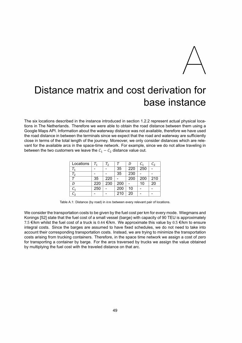
ADistance matrix and cost derivation for
base instanceThe six locations described in the instance introduced in section 1.2.2 represent actual physical loca-tions in The Netherlands. Therefore we were able to obtain the road distance between them using aGoogle Maps API. Information about the waterway distance was not available, therefore we have usedthe road distance in between the terminals since we expect that the road and waterway are sufficientlyclose in terms of the total length of the journey. Moreover, we only consider distances which are rele-vant for the available arcs in the space-time network. For example, since we do not allow traveling inbetween the two customers we leave the 𝐶 − 𝐶 distance value out.
Locations 𝑇 𝑇 𝑇 𝐷 𝐶 𝐶𝑇 - - 35 220 250 -𝑇 - - 35 230 - -𝑇 35 220 - 200 200 210𝐷 220 230 200 - 10 20𝐶 250 - 200 10 - -𝐶 - - 210 20 - -
Table A.1: Distance (by road) in between every relevant pair of locations.
We consider the transportation costs to be given by the fuel cost per km for every mode. Wiegmans andKonings [52] state that the fuel cost of a small vessel (barge) with capacity of 90 TEU is approximately7.5 €/km whilst the fuel cost of a truck is 0.44 €/km. We approximate this value by 0.5 €/km to ensureintegral costs. Since the barges are assumed to have fixed schedules, we do not need to take intoaccount their corresponding transportation costs. Instead, we are trying to minimize the transportationcosts arising from trucking containers. Therefore, in the space time network we assign a cost of zerofor transporting a container by barge. For the arcs traversed by trucks we assign the value obtainedby multiplying the fuel cost with the traveled distance on that arc.
49


Bibliography[1] European Gateway Services. URL http://www.europeangatewayservices.com/en/
about-egs/company-profile/. Accessed: 2018-02-08.
[2] Greenhouse gas emissions from transport. URL https://www.eea.europa.eu/data-and-maps/indicators/transport-emissions-of-greenhouse-gases/transport-emissions-of-greenhouse-gases-10/. Accessed: 2018-02-07.
[3] Platform Synchromodaliteit. URL http://www.synchromodaliteit.nl/. Accessed : 2018-02-06.
[4] Port Vision 2030. URL https://www.portofrotterdam.com/sites/default/files/upload/Port-Vision/Port-Vision-2030.pdf. Accessed: 2018-02-06.
[5] Elson Agastra, Giuseppe Pelosi, Stefano Selleri, and Ruggero Taddei. Taguchi's method formulti-objective optimization problems. International Journal of RF and Microwave Computer-Aided Engineering, 23(3):357–366, oct 2012. doi: 10.1002/mmce.20680. URL https://doi.org/10.1002/mmce.20680.
[6] Aaron Agbenyegah Agbo and Yanwei Zhang. Sustainable freight transport optimisation throughsynchromodal networks. Cogent Engineering, 4(1), dec 2017. doi: 10.1080/23311916.2017.1421005. URL https://doi.org/10.1080/23311916.2017.1421005.
[7] Agostinho Agra, Marielle Christiansen, Rosa Figueiredo, Lars Magnus Hvattum, Michael Poss,and Cristina Requejo. The robust vehicle routing problem with time windows. Computers &Operations Research, 40(3):856–866, mar 2013. doi: 10.1016/j.cor.2012.10.002. URLhttps://doi.org/10.1016/j.cor.2012.10.002.
[8] Agostinho Agra, Marielle Christiansen, Lars Magnus Hvattum, and Filipe Rodrigues. Robust op-timization for a maritime inventory routing problem. Transportation Science, 52(3):509–525, jun2018. doi: 10.1287/trsc.2017.0814. URL https://doi.org/10.1287/trsc.2017.0814.
[9] Faiz Al-Khayyal and Seung-June Hwang. Inventory constrained maritime routing and schedulingfor multi-commodity liquid bulk, part i: Applications and model. European Journal of OperationalResearch, 176(1):106–130, jan 2007. doi: 10.1016/j.ejor.2005.06.047. URL https://doi.org/10.1016/j.ejor.2005.06.047.
[10] Anonymous. EUROPA - EU transport policy, June 2016. URL https://europa.eu/european-union/topics/transport_en. Accessed: 2018-02-07.
[11] Ruibin Bai, SteinW.Wallace, Jingpeng Li, and Alain Yee-LoongChong. Stochastic service networkdesign with rerouting. Transportation Research Part B: Methodological, 60:50–65, feb 2014. doi:10.1016/j.trb.2013.11.001. URL https://doi.org/10.1016/j.trb.2013.11.001.
[12] Behzad Behdani, Yun Fan, Bart Wiegmans, and Rob Zuidwijk. Multimodal schedule design forsynchromodal freight transport systems. SSRN Electronic Journal, 2014. doi: 10.2139/ssrn.2438851. URL https://doi.org/10.2139/ssrn.2438851.
[13] A. Ben-Tal, A. Goryashko, E. Guslitzer, and A. Nemirovski. Adjustable robust solutions of un-certain linear programs. Mathematical Programming, 99(2):351–376, mar 2004. doi: 10.1007/s10107-003-0454-y. URL https://doi.org/10.1007/s10107-003-0454-y.
[14] Aharon Ben-Tal, Laurent El Ghaoui, and Arkadi Nemirovski. Robust Op-timization (Princeton Series in Applied Mathematics). Princeton Univer-sity Press, 2009. ISBN 0691143684. URL https://www.amazon.com/
51
52 Bibliography
Robust-Optimization-Princeton-Applied-Mathematics/dp/0691143684?SubscriptionId=0JYN1NVW651KCA56C102&tag=techkie-20&linkCode=xm2&camp=2025&creative=165953&creativeASIN=0691143684.
[15] Dimitris Bertsimas and Melvyn Sim. The price of robustness. Operations Research, 52(1):35–53,feb 2004. doi: 10.1287/opre.1030.0065. URL https://doi.org/10.1287/opre.1030.0065.
[16] John R. Birge and François Louveaux. Introduction to Stochastic Programming (Springer Series inOperations Research and Financial Engineering). Springer, 2011. URL https://www.amazon.com/Introduction-Stochastic-Programming-Operations-Engineering-ebook/dp/B00FBQZ2ZQ?SubscriptionId=AKIAIOBINVZYXZQZ2U3A&tag=chimbori05-20&linkCode=xm2&camp=2025&creative=165953&creativeASIN=B00FBQZ2ZQ.
[17] Y.M. Bontekoning, C. Macharis, and J.J. Trip. Is a new applied transportation research fieldemerging?––A review of intermodal rail–truck freight transport literature. Transportation ResearchPart A: Policy and Practice, 38(1):1–34, jan 2004. doi: 10.1016/j.tra.2003.06.001. URLhttps://doi.org/10.1016/j.tra.2003.06.001.
[18] Katrin Brümmerstedt, Hendrik Meyer-Van Beek, and Torsten Münsterberg. Comparative analysisof synchromodality in major european seaports. 2017. doi: 10.15480/882.1477.
[19] M. Caramia and F. Guerriero. A heuristic approach to long-haul freight transportation with multipleobjective functions. Omega, 37(3):600–614, jun 2009. doi: 10.1016/j.omega.2008.02.001.URL https://doi.org/10.1016/j.omega.2008.02.001.
[20] An Caris, CathyMacharis, andGerrit K. Janssens. Decision support in intermodal transport: A newresearch agenda. Computers in Industry, 64(2):105–112, feb 2013. doi: 10.1016/j.compind.2012.12.001. URL https://doi.org/10.1016/j.compind.2012.12.001.
[21] Tsung-Sheng Chang. Best routes selection in international intermodal networks. Computers &Operations Research, 35(9):2877–2891, sep 2008. doi: 10.1016/j.cor.2006.12.025. URLhttps://doi.org/10.1016/j.cor.2006.12.025.
[22] Jae Hyung Cho, Hyun Soo Kim, and Hyung RimChoi. An intermodal transport network planning al-gorithm using dynamic programming—a case study: from busan to rotterdam in intermodal freightrouting. Applied Intelligence, 36(3):529–541, mar 2010. doi: 10.1007/s10489-010-0223-6.URL https://doi.org/10.1007/s10489-010-0223-6.
[23] Mervat Chouman, Teodor Gabriel Crainic, and Bernard Gendron. Commodity representations andcut-set-based inequalities for multicommodity capacitated fixed-charge network design. Trans-portation Science, 51(2):650–667, may 2017. doi: 10.1287/trsc.2015.0665. URL https://doi.org/10.1287/trsc.2015.0665.
[24] Michele Conforti. Integer programming. Springer International Publishing Imprint Springer, 2014.ISBN 978-3-319-11008-0.
[25] Teodor Gabriel Crainic. Service network design in freight transportation. European Journal ofOperational Research, 122(2):272–288, apr 2000. doi: 10.1016/s0377-2217(99)00233-7.URL https://doi.org/10.1016/s0377-2217(99)00233-7.
[26] Teodor Gabriel Crainic and Tolga Bektas. Brief overview of intermodal transportation. In Lo-gistics Engineering Handbook, pages 28–1–28–16. CRC Press, dec 2007. doi: 10.1201/9780849330537.ch28. URL https://doi.org/10.1201/9780849330537.ch28.
[27] Teodor Gabriel Crainic and Kap Hwan Kim. Chapter 8 Intermodal Transportation. In Trans-portation, pages 467–537. Elsevier, 2007. doi: 10.1016/s0927-0507(06)14008-6. URLhttps://doi.org/10.1016/s0927-0507(06)14008-6.
[28] Teodor Gabriel Crainic and Gilbert Laporte. Planning models for freight transportation. Europeanjournal of operational research, 97(3):409–438, 1997.
Bibliography 53
[29] Union Européenne and Commission Européenne. EU transport in figures 2016. Publicationsoffice of the European Union, Luxembourg, 2016. ISBN 978-92-79-51528-6. OCLC: 960914234.
[30] Reza Zanjirani Farahani, Masoud Hekmatfar, Alireza Boloori Arabani, and Ehsan Nikbakhsh. Hublocation problems: A review of models, classification, solution techniques, and applications. Com-puters & Industrial Engineering, 64(4):1096–1109, apr 2013. doi: 10.1016/j.cie.2013.01.012.URL https://doi.org/10.1016/j.cie.2013.01.012.
[31] Martijn R. van der Horst and Peter W. de Langen. Coordination in hinterland transport chains:A major challenge for the seaport community. Maritime Economics & Logistics, 10(1-2):108–129, mar 2008. doi: 10.1057/palgrave.mel.9100194. URL https://doi.org/10.1057/palgrave.mel.9100194.
[32] Dylan Huizing. General methods for synchromodal planning of freight containers and transports.Master’s thesis, Delft University of Technology, 2017.
[33] M. A. M. De Juncker, D. Huizing, M. R. Ortega del Vecchyo, F. Phillipson, and A. Sangers. Frame-work of synchromodal transportation problems. In Lecture Notes in Computer Science, pages383–403. Springer International Publishing, 2017. doi: 10.1007/978-3-319-68496-3_26. URLhttps://doi.org/10.1007/978-3-319-68496-3_26.
[34] Kishan Kalicharan. Intermodal transport: Routing vehicles and scheduling containers. Master’sthesis, Delft University of Technology, 2018.
[35] Kees Kooiman, Frank Phillipson, and Alex Sangers. Planning inland container shipping:A stochastic assignment problem. In Analytical and Stochastic Modelling Techniques andApplications, pages 179–192. Springer International Publishing, 2016. doi: 10.1007/978-3-319-43904-4_13. URL https://doi.org/10.1007/978-3-319-43904-4_13.
[36] Albert Madansky. Methods of solution of linear programs under uncertainty: notes on linear pro-gramming and extensions-part 56. Technical report, Santa Monica, CA: RAND Corporation. URLhttps://www.rand.org/pubs/research_memoranda/RM2752.html.
[37] Max Roberto Ortega Del Vecchyo. Container-to-mode assignment on a synchromodal transporta-tion network: a multi-objective approach. Master’s thesis, Delft University of Technology, 2017.
[38] Sarah Pfoser, Horst Treiblmaier, and Oliver Schauer. Critical Success Factors of Synchromodality:Results from a Case Study and Literature Review. Transportation Research Procedia, 14:1463–1471, 2016. ISSN 23521465. doi: 10.1016/j.trpro.2016.05.220. URL http://linkinghub.elsevier.com/retrieve/pii/S2352146516302228.
[39] Arturo E. Pérez Rivera and Martijn R. K. Mes. Scheduling drayage operations in synchromodaltransport. In Lecture Notes in Computer Science, pages 404–419. Springer International Pub-lishing, 2017. doi: 10.1007/978-3-319-68496-3_27. URL https://doi.org/10.1007/978-3-319-68496-3_27.
[40] Arturo Pérez Rivera and Martijn Mes. Service and transfer selection for freights in a synchromodalnetwork. In Lecture Notes in Computer Science, pages 227–242. Springer International Pub-lishing, 2016. doi: 10.1007/978-3-319-44896-1_15. URL https://doi.org/10.1007/978-3-319-44896-1_15.
[41] K. Sharypova. Optimization of hinterland intermodal container transportation. PhD thesis, TUE :Department of Industrial Engineering and Innovation Sciences, 2014.
[42] P.M. Singh, M.J van Sinderen, and R.J Wieringa. Synchromodal transport: Pre-requisites, ac-tivities and effects. In Informations Systems, Logistics, and Supply Chain. Springer InternationalPublishing, 2016.
[43] Prince Mayurank Singh and Marten J. van Sinderen. Interoperability challenges for context awarelogistics services - the case of synchromodal logistics, page 9. CEUR Workshop Proceedings.CEUR-WS.org, 2015. Interoperability, Context-aware, Logistics, Synchromodal.
54 Bibliography
[44] M. SteadieSeifi, N.P. Dellaert, W. Nuijten, T. Van Woensel, and R. Raoufi. Multimodal freighttransportation planning: A literature review. European Journal of Operational Research, 233(1):1–15, February 2014. ISSN 03772217. doi: 10.1016/j.ejor.2013.06.055. URL http://linkinghub.elsevier.com/retrieve/pii/S0377221713005638.
[45] Agachai Sumalee, Kenetsu Uchida, and William H.K. Lam. Stochastic multi-modal trans-port network under demand uncertainties and adverse weather condition. Transportation Re-search Part C: Emerging Technologies, 19(2):338–350, April 2011. ISSN 0968090X. doi:10.1016/j.trc.2010.05.018. URL http://linkinghub.elsevier.com/retrieve/pii/S0968090X10001026.
[46] Yan Sun, Maoxiang Lang, and Danzhu Wang. Optimization models and solution algorithmsfor freight routing planning problem in the multi-modal transportation networks: A review of thestate-of-the-art. The Open Civil Engineering Journal, 9(1):714–723, sep 2015. doi: 10.2174/1874149501509010714. URL https://doi.org/10.2174/1874149501509010714.
[47] Lorant A. Tavasszy, Behzad Behdani, and Rob Konings. Intermodality and synchromodality. SSRNElectronic Journal, 2015. doi: 10.2139/ssrn.2592888. URL https://doi.org/10.2139/ssrn.2592888.
[48] Roy Van den Berg and Peter W. De Langen. An exploratory analysis of the effects of modalsplit obligations in terminal concession contracts. International Journal of Shipping and TransportLogistics, 6(6):571–592, 2014.
[49] Bart van Riessen, Rudy R. Negenborn, and Rommert Dekker. Synchromodal Container Trans-portation: An Overview of Current Topics and Research Opportunities. In Francesco Corman,Stefan Voß, and Rudy R. Negenborn, editors, Computational Logistics, volume 9335, pages386–397. Springer International Publishing, Cham, 2015. ISBN 978-3-319-24263-7 978-3-319-24264-4. URL http://link.springer.com/10.1007/978-3-319-24264-4_27. DOI:10.1007/978-3-319-24264-4_27.
[50] Kees Verweij. Synchronic modalities - critical success factors. Logistics Handbook 2011, 2011.
[51] Nicole Wieberneit. Service network design for freight transportation: a review. OR Spectrum,30(1):77–112, mar 2007. doi: 10.1007/s00291-007-0079-2. URL https://doi.org/10.1007/s00291-007-0079-2.
[52] Bart Wiegmans and Rob Konings. Intermodal inland waterway transport: Modelling conditionsinfluencing its cost competitiveness. The Asian Journal of Shipping and Logistics, 31(2):273–294,jun 2015. doi: 10.1016/j.ajsl.2015.06.006. URL https://doi.org/10.1016/j.ajsl.2015.06.006.
[53] Wang X., Crainic T. G., and Wallace S. Stochastic scheduled service network design: the valueof deterministic solutions. Technical report, CIRRELT, CIRRELT-2016-14, 2016.
[54] Guiwu Xiong and Yong Wang. Best routes selection in multimodal networks using multi-objectivegenetic algorithm. Journal of Combinatorial Optimization, 28(3):655–673, dec 2012. doi: 10.1007/s10878-012-9574-8. URL https://doi.org/10.1007/s10878-012-9574-8.
[55] İhsan Yanıkoğlu, Bram L. Gorissen, and Dick den Hertog. A Survey of Adjustable Robust Opti-mization. European Journal of Operational Research, (to appear), 2017.
[56] M. Zhang and A.J. Pel. Synchromodal hinterland freight transport: Model study for the port ofrotterdam. Journal of Transport Geography, 52:1–10, apr 2016. doi: 10.1016/j.jtrangeo.2016.02.007. URL https://doi.org/10.1016/j.jtrangeo.2016.02.007.
Related Documents


![Low Cost, Robust and Real Time System for Detecting …-Robust-and-Real-Time...2 DATMO System for Automatic Cargo Handling in Port Terminals terminals [13]. Therefore, Automated Container](https://static.cupdf.com/doc/110x72/5ae651d17f8b9a9e5d8d91c6/low-cost-robust-and-real-time-system-for-detecting-robust-and-real-time2.jpg)