A Robust Algorithm for A Robust Algorithm for Approximate Compatible Approximate Compatible Observability Don’t Care Observability Don’t Care (CODC) Computation (CODC) Computation Nikhil S. Saluja University of Colorado Boulder, CO Sunil P. Khatri Texas A&M University, College Station, TX

A Robust Algorithm for Approximate Compatible Observability Don’t Care (CODC) Computation Nikhil S. Saluja University of Colorado Boulder, CO Sunil P.
Dec 19, 2015
Welcome message from author
This document is posted to help you gain knowledge. Please leave a comment to let me know what you think about it! Share it to your friends and learn new things together.
Transcript

A Robust Algorithm for A Robust Algorithm for Approximate Compatible Approximate Compatible Observability Don’t Care Observability Don’t Care
(CODC) Computation(CODC) Computation
Nikhil S. SalujaUniversity of Colorado
Boulder, CO
Sunil P. KhatriTexas A&M University,
College Station, TX

OutlineOutline
Motivation Computation of Don’t Cares ACODC Algorithm
Proof of correctness
Experimental Results Possible extensions Conclusions

MotivationMotivation
…
…..
…..
z1 z2 z3 zp
x1 x2 x3 xn
yj = Fj
y1 y2yw
n mSDC B ( )
( )jj INT
SDC SDC
( )j j jSDC y F ( )k kXDC G x
( )k PO
( )k
k PO
XDC XDC
( )k
jkj
zODC
y
( )j jk
k PO
ODC ODC
Technology independent logic optimization Typically compute Don’t Cares after a higher level description of a design is encoded and translated into gate level description. Don’t Cares (DCs)
eXternal Don’t Cares (XDCs) Satisfiability Don’t Cares (SDCs) Observability Don’t Cares (ODCs)
1
( )p
j j jk kk
DC SDC ODC XDC

Motivation - 2Motivation - 2
The DCs computed are a function of the PIs and internal variables of the Boolean network Image computation used to express the DCs in
terms of node fanins ROBDD based operation
Finally, the node function is minimized (using ESPRESSO) with respect to the computed (local) DCs
Literal count reduction is the figure of merit

Don’t CaresDon’t Cares ODC based
Very powerful, represent maximum flexibility Minimizing a node j with respect to its ODC requires recomputation of other nodes’ ODCs
Compatible ODC (CODC) based Subset of ODC, requires ordering of fanins Recomputation not required, useful in many cases
In either case, image computation required To obtain DCs in the fanin support of the node Involves ROBDD computation
Not robust

Note that is the consensus operator The first fanin has
which is the maximum flexibility A new edge eik should have its CODC as the conjunction of with the condition that other inputs j < i are not insensitive to input yj ( ) or are independent of yj ( )
CODC ComputationCODC Computation Traverse circuit in reverse topological order
CODC of primary output z initialized to its XDC
Computation performed in 2 phases for each node Phase 1
11
kk k
fCODC CODC
y
yk
fk
y1
y2yi-1
yi
y1 < y2 < … < yi
k
i
ky
i
ky
kik CODC
y
fC
y
fC
y
fCODC
i
))...((11
11
iFOk
iki CODCCODC
jyC
k
i
f
y
k
j
f
y
jyC

CODC ComputationCODC Computation Phase 2 - image computation using ROBDDs
Build global BDDs of each node in the network, including POs
For large circuits this step fails This is the main weakness of the CODC computation
Next compute CODCs of node k in terms of PIs Substitute each internal node literal by its global BDD
Compute image of this function in the space of local fanins of node k
Yields CODC in terms of local fanins of node k
Finally, call ESPRESSO on the cover of node k, with the newly computed CODC as don’t care

Contributions of this Contributions of this WorkWork
Perform CODC based Don’t Care computation approximately Yields 25X speedup Yields 33X reduction in memory utilization Obtains 80% of the literal reduction of the full
CODC computation Handles large circuits extremely fast (circuits
which CODC based computation times out on) Formal proof of correctness of the approximate
CODC technique

Approximate CODCsApproximate CODCs
Consider a sub-network rooted at the node j of interest
Sub-network can have user defined topological depth k
Compute the CODC of j in the sub-network (called ACODC)
This ACODC is a subset of the CODC of j
jjjj
j

AlgorithmAlgorithm
Traverse η in reverse topological order
for (each node j in network η) do
ηj = extract_subnetwork(j,k)
ACODC(j) = compute_acodc(ηj,j)
optimize(j,ACODC(j))
end for

Proof of CorrectnessProof of Correctness
Terminology Boolean network ηxz X primary inputs Z primary outputs W and V are two cuts ηxw, ηvz and ηvw define sub-networks is the CODC of yk where P is either X
or V and Q is either W or Z is the CODC of yk mapped back to its
fanin support after image computation
PQkCODC
FIPQkCODC ,
v wx z
y1
y2
yi-1yi
ykfk

Cutset as Primary Cutset as Primary OutputOutput
To show ≥ For any PO z, = ø For , ≠ ø For W nodes as POs, = ø CODC computation of yk is identical for both
cases except last term in equation
In general, the last term for a node in first case, contains last term for same node in latter case since ≥
Hence ≥
FIXZzCODC ,
FIXZwCODC ,Ww
FIXWwCODC ,
k
i
ky
i
ky
kik CODC
y
fC
y
fC
y
fCODC
i
))...((11
11
FIXZwCODC , FIXW
wCODC ,
FIXWkCODC ,FIXZ
kCODC ,
w
x
z
yk
fk
y1
y2yi-1
yi
FIXWkCODC ,FIXZ
kCODC ,

Cutset as Primary InputCutset as Primary Input Define To compute ACODC at yk, compute ,
then compute image I1 of this on the V space, and then project the result back to local fanins of yk
The full CODC is .We then compute the image I2 of this on the X space, and next project the result back to local fanins of yk
I3 is projection of I2 on V
Hence Therefore I3 ≥ I1
Finally, ≥
v
x
z
yk
fk
y1
y2yi-1
yi
Vi ii XvvXVR )(),(
VZkCODC
XZkCODC
3 1 2( ( , ) ( ))XI I R V X I X
FIVZkCODC ,FIXZ
kCODC ,
I1
I2
I3
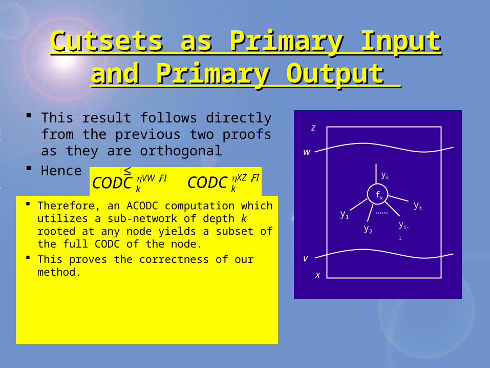
Cutsets as Primary Input Cutsets as Primary Input and Primary Output and Primary Output
This result follows directly from the previous two proofs as they are orthogonal
Hence ≤
w
x
z
yk
fk
y1
y2yi-1
yi
v
FIVWkCODC , FIXZ
kCODC ,
Therefore, an ACODC computation which utilizes a sub-network of depth k rooted at any node yields a subset of the full CODC of the node.
This proves the correctness of our method.
Experimental ResultsExperimental Results Implemented in SIS Used mcnc91 and itc99 benchmark circuits Run on IBM IntelliStation (1.7 GHz Pentium-
4 with 1 GB RAM) running Linux Our algorithm is built as a replacement to
full_simplify Read design and run ACODC algorithm followed
by sweep Compare our method by running full_simplify
followed by sweep

Metrics for ComparisonMetrics for Comparison 3 measures of effectiveness for comparison with
full_simplify Effectiveness #1 compares the ratio of the number of minterms
computed by our technique compared to that for full_simplify
Effectiveness #2 compares the number of nodes for which ACODCs and CODCs are identical
We also compare the literal count reduction obtained by both techniques
| ( ) |
#1| ( ) |
j
j
ACODC j
effectivenessCODC j
##2
#
equaleffectiveness
total

Effectiveness ResultsEffectiveness ResultsCircuit Eff1 (k=4) Eff1 (k=6) Eff2 (k=4) Eff2 (k=6) Lits-original Lits % (fs) Lits % (k=4) Lits % (k=6)
C1355 98.04 98.04 98.34 98.34 1032 4.65 3.88 3.88
C1908 81.56 84.69 87.13 88.89 1497 37.14 30.66 31.46
C2670 94.13 94.13 86.79 86.79 2043 39.30 32.94 32.94
C432 71.43 71.43 92.81 92.81 372 19.89 9.95 9.95
C499 98.56 98.56 97.34 97.34 616 7.79 6.50 6.50
C880 80.00 84.44 94.56 95.77 703 11.10 9.67 10.38
C3540 85.43 97.81 84.15 97.51 2934 33.78 26.89 28.42
dalu 78.00 79.86 75.78 79.55 3588 39.68 9.70 9.70
i10 99.34 99.34 85.45 85.45 5376 29.55 27.47 27.47
b01_C 92.68 92.68 83.33 83.33 80 45.00 43.75 43.75
b03_C 68.89 75.56 87.23 89.43 254 60.00 39.37 41.34
b04_C 63.42 63.42 85.35 85.35 1267 31.96 28.65 28.65
b05_C 74.70 84.85 76.38 88.02 1858 45.80 14.96 14.96
b06_C 92.11 92.11 87.10 87.10 83 51.80 45.78 45.78
b07_C 69.52 81.90 91.02 95.21 749 11.88 11.08 11.08
b08_C 98.33 98.33 96.09 96.09 306 9.80 9.48 9.48
b09_C 79.00 95.00 83.04 90.18 277 61.00 44.04 45.85
b10_C 80.65 83.87 92.90 94.19 353 12.39 11.05 11.05
b11_C 83.44 85.94 89.50 91.65 1378 22.71 14.36 14.36
b12_C 67.10 79.04 87.17 90.92 1967 24.05 5.80 5.80
b13_C 65.08 65.08 91.53 91.53 558 18.81 10.57 10.57
AVG 81.97 85.52 87.85 89.52 - 28.36 22.34 22.82
Literal reduction about 80% of full_simplify Very little improvement from k=4 to k=6

Runtime is about 25X better than full_simplify Memory utilization is about 33X better than full_simplify
Runtime and Memory Runtime and Memory ResultsResults
Circuit Time (fs) Time % (k=4) Time % (k=6)
C1355 39.28 1.66 1.80
C1908 54.68 2.40 2.50
C2670 11.77 4.20 4.66
C432 4.91 1.25 1.45
C499 2.41 1.20 1.31
C880 2.05 0.70 0.72
C3540 835.64 25.25 27.45
dalu 210.09 6.23 7.12
i10 332.22 8.56 9.21
b01_C 0.03 0.05 0.05
b03_C 0.19 0.20 0.20
b04_C 12.15 1.47 1.66
b05_C 24.50 2.43 2.50
b06_C 0.04 0.04 0.04
b07_C 4.04 0.84 0.86
b08_C 0.30 0.30 0.30
b09_C 0.37 0.26 0.27
b10_C 0.40 0.30 0.32
b11_C 9.97 0.26 0.34
b12_C 81.72 3.23 3.55
b13_C 0.28 0.20 0.21
AVG - 0.037 0.041
Mem (fs) Mem (k=4) Mem (k=6)
312732 3066 3066
106288 3066 3066
172718 4088 4088
289226 6132 6132
99134 8176 8176
73584 2044 3066
321746 8176 8176
499758 11242 12264
507934 4088 4088
1022 1022 1022
1022 1022 1022
117530 2044 3066
25550 5110 5110
1022 1022 1022
26572 2044 2044
2044 2044 2044
1022 1022 1022
2044 1022 1022
22484 2044 2044
15330 4088 4088
2044 1022 1022
- 0.028 0.032

Circuit #Nodes #Literals Node% Lit% Time(s) Mem
C6288 2416 4800 4.39 3.69 3.65 1022
C7552 3466 6098 40.68 26.15 6.11 9198
b14 9768 18917 17.15 10.12 117.60 105582
b14_1 6570 12886 20.03 9.56 19.04 50078
b20 19683 38213 18.64 8.68 65.39 69496
b20_1 13900 27074 18.96 8.95 39.34 34748
b21 20028 38993 17.91 8.48 66.37 65408
b21_1 13899 27164 17.56 9.45 38.32 34748
AVG - - 18.77 9.49 - -
Results for Large Results for Large CircuitsCircuits
full_simplify did not complete for all the examples below k = 4 for these experiments
Maximum runtime < 2 minutes
Peak memory utilization < 106K BDD nodes

Possible ExtensionsPossible Extensions
Can compute AODCs in a similar fashion Yields more flexibility at a node However, each node must be minimized after
its AODC computation Compatibility not maintained
Useful if only node minimization is desired Compatibility is useful if the nodes are to be
optimized simultaneously at a later stage
Proof of correctness is similar

ConclusionsConclusions
Presented a robust technique for ACODC computation
Dynamic extraction of sub-networks to compute CODCs
ACODCs computed exactly once for a node 19% reduction in node count and 9.5% reduction
in literal count (large circuits) 23% reduction in literal count as compared to
28.5% for full_simplify (medium circuits) 25X better run-time than full_simplify 33X better memory utilization than full_simplify
Related Documents