A revised hydrology for the ECMWF model: Verification from field ...

563

A revised hydrology for the ECMWFmodel: Verification from field site toterrestrial water storage and impact

in the Integrated Forecast System

G. Balsamo1, P. Viterbo2, A. Beljaars1,B. van den Hurk3, M. Hirschi4,

A. K. Betts5, K. Scipal1

Research Department

1ECMWF, UK, 2IM, Lisbon, Portugal,3 KNMI, DeBilt, The Netherlands, 4ETH-Zurich, Switzerland,

5Atmospheric Research, Pittsford, Vermont, USA

submitted to Journal of Hydrometeorology

April 2008

Series: ECMWF Technical Memoranda

A full list of ECMWF Publications can be found on our web site under:http://www.ecmwf.int/publications/

Contact: [email protected]

c©Copyright 2008

European Centre for Medium-Range Weather ForecastsShinfield Park, Reading, RG2 9AX, England

Literary and scientific copyrights belong to ECMWF and are reserved in all countries. This publication is notto be reprinted or translated in whole or in part without the written permission of the Director. Appropriatenon-commercial use will normally be granted under the condition that reference is made to ECMWF.

The information within this publication is given in good faith and considered to be true, but ECMWF acceptsno liability for error, omission and for loss or damage arising from its use.

http://www.ecmwf.int/publications/

A revised hydrology for the ECMWF model

Abstract

The Tiled ECMWF Scheme for Surface Exchanges over Land (TESSEL) is used operationally in the Inte-grated Forecast System (IFS) for describing the evolution of soil, vegetation and snow over the continents atdiverse spatial resolutions. A revised land surface hydrology (HTESSEL) is introduced in the ECMWF op-erational model, to address shortcomings of the land surface scheme, specifically the lack of surface runoffand the choice of a global uniform soil texture. New infiltration and runoff schemes are introduced with adependency on the soil texture and standard deviation of orography. A set of experiments in stand-alonemode is used to assess the improved prediction of soil moisture at local scale against field site observations.Comparison with Basin-Scale Water Budget (BSWB) and Global Runoff Data Centre (GRDC) datasets indi-cates a consistently larger dynamical range of land water mass over large continental areas, and an improvedprediction of river runoff, while the impact on atmospheric fluxes is fairly small. Finally the ECMWF dataassimilation and prediction systems are used to verify the impact on surface and near-surface quantities inatmospheric-coupled mode. A mid-latitude error reduction is seen both in soil moisture and in 2m tempera-ture.

1. Introduction

A correct representation of the soil water buffering in land surface schemes used for weather and climateprediction is essential to accurately simulate surface water fluxes both towards the atmosphere and rivers (vanden Hurk et al., 2005; Hirschi et al., 2006a). Moreover the energy repartition at the surface is largely driven bythe soil moisture which influences directly the Bowen ratio.

The introduction of a revised hydrology in the Tiled ECMWF Scheme for Surface Exchanges over Land (TES-SEL) has been investigated by van den Hurk and Viterbo (2003) for the Baltic basin. These model developmentswere a response to known weaknesses of the TESSEL hydrology: specifically the choice of a single global soiltexture, which does not characterize different soil moisture regimes, and a Hortonian runoff scheme whichproduces hardly any surface runoff. A revised formulation of the soil hydrological conductivity and diffusivity,spatially variable according to a global soil texture map, and surface runoff based on the variable infiltrationcapacity approach, are the proposed remedies.

Offline (or stand-alone) verification is a convenient framework for isolating the benefits of a given land surfaceparameterization. A set of field site experiments and two land surface intercomparison experiments over largedomains are considered. A Sahelian site and a Boreal forest site have been chosen to show relevant effectsof the new hydrology. Two major land surface intercomparison experiments, the Global Soil Wetness Project,Second initiative, GSWP-2 (Dirmeyer et al., 1999, 2002; Gao et al., 2004) and the Rhone Aggregation Project,RhoneAgg (Boone et al., 2004), provided spatialized near-surface forcing for land surface models, and havebeen re-run with the new scheme to evaluate the water budget for accumulated quantities. In the GSWP-2 simulations, both terrestrial water storage estimates and the river discharge are examined on a number ofbasins. Hydrological consistency on the monthly time-scale is verified. The RhoneAgg simulation are used toexamine the fast component of runoff at the daily time-scale.

The coupling between the land surface and the atmosphere is then also evaluated. This is an essential step,since Koster et al. (2004) indicated a strong inter-model variability in coupling between soil moisture andprecipitation over large continental areas, generalizing the studies of Beljaars et al. (1996).

In order to assess the impact of the new parameterization, a set of long-term atmospheric coupled integrations(13-month) with specified Sea-Surface-Temperature is produced. This configuration, named climate simulationallows evaluating surface-atmosphere feedbacks and focusing on the impact of the land surface modification.Annual and seasonal averages are compared to a number of independent datasets with a focus on boreal summermonths when a larger impact of the soil hydrology is expected. Finally, since in the NWP application the

Technical Memorandum No. 563 1


coupled system is subject to cyclic correction by data assimilation, an overall assessment is provided by thecomparison of the land surface analysis increments in the old and new version of the land surface model. Areduction of increments between the two model versions can be interpreted as an overall improvement of theland surface representation. In this case the soil moisture increments are considered in a long (7-month) dataassimilation experiment.

In section 2 the hydrology of the TESSEL land surface scheme and the HTESSEL (Hydrology TESSEL)revision are illustrated. Sensitivity experiments are realized to show the impact of the new parameterizationon surface runoff and soil water transfer. Section 3 evaluates the soil moisture range associated with the newphysiographic values (for the permanent wilting point and the soil field capacity) for a number of sites andpresents the validation results at two contrasting field sites that illustrate the main behaviour of the HTESSELand TESSEL scheme. In section 4, the regional to global offline simulations are introduced, together withthe main verification datasets provided by the Basin-Scale Water Budget, BSWB (Seneviratne et al., 2004)the Global Runoff Data Centre, GRDC (Fekete et al., 2000) and the ERA-40 reanalysis (Uppala et al., 2005)datasets.

Results of atmospheric-coupled simulations and data assimilation experiments are presented and discussed insection 5 together with the relevant lessons learnt from the ERA-40 reanalysis. A summary of the changes andthe conclusions are then provided in the last section, while the datasets for the global implementation of therevised hydrology scheme are presented in the Appendix.

2. TESSEL hydrology

The TESSEL scheme (Tiled ECMWF Scheme for Surface Exchanges over Land) is shown schematically inFigure 1a. Up to six tiles are present over land (bare ground, low and high vegetation, intercepted water, shadedand exposed snow) and 2 over water (open and frozen water) with separate energy and water balances. The

Schematics of the land surface

a)

b)

interceptionreservoir

lowvegetation

bareground

snow onground & low

vegetationhigh

vegetationsnow under

high vegetation

ra

rc1 rc1rc2 rasrs

ra ra ra ra

Figure 1: Schematic representation of the structure of (a) TESSEL land-surface scheme and (b) spatial structure addedin HTESSEL (for a given precipitation P1 = P2 the scheme distributes the water as surface runoff and drainage withfunctional dependencies on orography and soil texture respectively).

2 Technical Memorandum No. 563


vertical discretization considers a four-layer soil that can be covered by a single layer of snow. The depthsof the soil layers are in an approximate geometric relation, as suggested in Deardorff (1978). Warrilow et al.(1986) have shown that four layers provide a reasonable compromise between computational cost and theability to represent all timescales between one day and a year. The soil heat budget follows a Fourier diffusionlaw, modified to take into account soil water freezing/melting according to Viterbo et al. (1999). The energyequation is solved with a net ground heat flux as the top boundary condition and a zero-flux at the bottom. Aninterception layer accumulates precipitation until it is saturated, and the remaining precipitation (throughfall)is partitioned between surface runoff and infiltration. Subsurface water fluxes are determined by Darcy’s law,used in a soil water equation solved with a four-layer discretization shared with the heat budget equation. Thetop boundary condition is infiltration plus surface evaporation, free drainage is assumed at the bottom and eachlayer has an additional sink of water in the form of root extraction over vegetated areas.

In each grid box two vegetation types are present: a high and a low vegetation type. An external climatedatabase is used to obtain the vegetation characteristics, based on the Global Land Cover Characteristics(GLCC) data (Loveland et al., 2000), http://edcsns17.cr.usgs.gov/glcc/. The nominal reso-lution is 1 km. The data provides for each pixel a biome classification based on the Biosphere-AtmosphereTransfer Scheme (BATS) model (Dickinson et al., 1993), and four parameters have been derived for each gridbox: dominant vegetation type, TH and TL, and the area fraction, AH and AL, for each of the high- and low-vegetation components, respectively.

The vertical movement of water in the unsaturated zone of the soil matrix obeys the following equation(Richards, 1931; Philip, 1957; Hillel, 1982; Milly, 1982) for the volumetric water content θ :

ρw∂θ

∂ t=−∂Fw

∂ z+ρwSθ (1)

where ρw is the water density (kg m−3),Fw is the water flux in the soil (positive downwards, kg m−2s−1), and Sθ

is a volumetric sink term associated to root uptake (m3m−3s−1), which depends on the surface energy balanceand the root profile (Viterbo and Beljaars, 1995).

The liquid water flow, Fw, obeys Darcy’s law, written as

Fw =−ρw

(λ

∂θ

∂ z− γ

)(2)

where λ (m2 s−1) and γ (m s−1) are the hydraulic diffusivity and hydraulic conductivity, respectively.

Replacing (2) in (1), and defining parametric relations for λ and γ as functions of soil water, a partial differentialequation for θ is obtained:

∂θ

∂ t=

∂

∂ z

(λ

∂θ

∂ z− γ

)+Sθ (3)

The top boundary condition is given by precipitation plus snow melt minus bare ground evaporation minus sur-face runoff. The bottom boundary condition assumes free drainage. Abramopoulos et al. (1988) specified freedrainage or no drainage, depending on a comparison of a specified geographical distribution of bedrock depth,with a model-derived water-table depth. For the sake of simplicity the assumption of no bedrock everywherehas been adopted.

TESSEL adopts the Clapp and Hornberger (1978) formulation of hydraulic conductivity and diffusivity as afunction of soil-water content (see also Mahrt and Pan 1984 for a comparison of several formulations and


http://edcsns17.cr.usgs.gov/glcc/


Cosby et al. 1984 for further analysis)

γ = γsat

(θ

θsat

)2bc+3

λ =bcγsat(−ψsat)

θsat

(θ

θsat

)bc+2 (4)

where bc is a non-dimensional exponent, γsat and ψsat are the values of the hydraulic conductivity and matricpotential at saturation. A minimum value is assumed for λ and γ corresponding to permanent wilting-pointwater content.

Cosby et al. (1984) tabulate best estimates of bc, γsat, ψsat and θsat, for the 11 soil classes of the US Departmentof Agriculture (USDA) soil classification, based on measurements over large samples. Viterbo and Beljaars(1995) adopted an averaging procedure to calculate for a medium-textured (loamy) soil used in TESSEL thevalues of γsat = 0.57×10−6 m s−1, bc = 6.04, and ψsat =−0.338 m, compatible with the Clapp and Hornbergerexpression for the matric potential

ψ = ψsat

(θ

θsat

)−bc

(5)

with ψ(θpwp) =−153 m (−15 bar) and ψ(θcap) =−3.37 m (−0.33 bar) (following Hillel 1982 and Jacqueminand Noilhan 1990).

The water transport in frozen soil is limited in the case of a partially frozen soil, by considering the effectivehydraulic conductivity and diffusivity to be a weighted average of the values for total soil water and a verysmall value (for convenience, taken as the value of (Eq. 4) at the permanent wilting point) for frozen wateras detailed in Viterbo et al. (1999). The soil properties, as defined above, also imply a maximum infiltrationrate at the surface defined by the maximum downward diffusion from a saturated surface. In general when thewater flux at the surface exceeds the maximum infiltration rate, the excess water is put into surface runoff. Thegeneral formulation of surface runoff can be written as:

R = T +M− Imax (6)

where Imax is the maximum infiltration rate, T the throughfall precipitation and M the snow melting. Differentrunoff schemes differ in the formulation of the infiltration. The maximum infiltration or Hortonian runoff,represent the runoff process at local scales. In TESSEL the maximum infiltration rate Imax is calculated as

Imax = ρw

(bcγsat(−ψsat)

θsat

θsat −θ1

z1/2+ γsat

)(7)

where ρw is the water density, and z1 is the depth of the first soil model layer (7 cm). At typical NWP modelresolutions this scheme is active only in the presence of frozen soil, when downward soil water transfer isinhibited, otherwise it hardly ever produces runoff, as shown in Boone et al. (2004).

a. The HTESSEL revision

The HTESSEL scheme includes the following revisions to the soil hydrology: (i) a spatially varying soil typereplacing the single loamy soil, (ii) the Van Genuchten (VG) formulation of soil hydraulic properties replacingthe Clapp and Hornberger (CH) scheme, and (iii) the surface runoff generation changing according to a variableinfiltration capacity based on soil type and local topography.



Table 1: Van Genuchten soil parameters.Texture α l n γsatUnits m−1 - - 10−6m/sCoarse 3.83 1.250 1.38 6.94Medium 3.14 -2.342 1.28 1.16Medium-Fine 0.83 -0.588 1.25 0.26Fine 3.67 -1.977 1.10 2.87Very Fine 2.65 2.500 1.10 1.74Organic 1.30 0.400 1.20 0.93

Table 2: Values for the volumetric soil moisture in Van Genuchten and Clapp-Hornberger (CH, loamy; bottom row),at saturation, θsat , field capacity, θcap, and permanent wilting point, θpwp. Last column reports the plant available soilmoisture. Units are [m3m−3].

Texture θsat θcap θpwp θcap−θpwp

Coarse 0.403 0.244 0.059 0.185Medium 0.439 0.347 0.151 0.196Medium-Fine 0.430 0.383 0.133 0.251Fine 0.520 0.448 0.279 0.170Very Fine 0.614 0.541 0.335 0.207Organic 0.766 0.663 0.267 0.396Loamy (CH) 0.472 0.323 0.171 0.151

In Figure 1b the HTESSEL changes are illustrated: in two adjacent model grid-points with the same land surfaceconditions and receiving an equal amount of precipitation the surface runoff will be different and proportionalto the terrain complexity while the soil water drainage will depend on the soil texture class.

The van Genuchten (1980) formulation provides a closed-form analytical expression for the conductivity, givenas a function of the pressure head, h, as

γ = γsat[(1+αhn)1−1/n−αhn−1]2

(1+αhn)(1−1/n)(l+2) (8)

where α , n and l are soil-texture dependent parameters. Pressure head h is linked to the soil moisture by theexpression

θ(h) = θr +θsat −θr

(1+αh)1−1/n (9)

The VG scheme is recognized among soil physicists as capable of reproducing both the soil water retention andthe hydraulic conductivity, and has shown good agreement with observations in intercomparison studies (Shaoand Irannejad, 1999). Table 1 lists parameter values for six soil textures for the VG scheme. HTESSEL usesthe dominant soil texture class for each gridpoint. This information is taken from the FAO (FAO, 2003) datasetas detailed in the Appendix. The permanent wilting point and the soil field capacity are obtained by a specifiedmatric potential of ψ(θpwp) = −15bar and ψ(θcap) = −0.10bar, respectively. In Table 2 the volumetric soilmoistures associated with each soil class are shown for saturation, field capacity and wilting point. Also shownis the plant available water content and the percentage of land points in each class. The last row shows thecorresponding values for the single loamy soil used in the CH formulation in TESSEL. Note that the plantavailable soil water is greater for all the new soil classes in HTESSEL. Figure 2 shows the soil hydraulicdiffusivity and conductivity for the TESSEL CH formulation and the six VG soil texture classes in HTESSEL.In TESSEL those were not allowed to fall below their wilting point values. At saturation, TESSEL has thehighest diffusivity and conductivity. The reduced values for fine soils in HTESSEL reduces the infiltration ofwater and consequently the baseflow.



0 0.1 0.2 0.3 0.4 0.5 0.6 0.7 0.8 0 0.1 0.2 0.3 0.4 0.5 0.6 0.7 0.8Volumetric soil moisture, [m3m–3] Volumetric soil moisture, [m3m–3]

10–1

10–2

10–3

10–4

10–5

10–6

10–7

10–8

10–9

10–10

10–11

10–12

10–13

10–14

10–15

10–1

10–2

10–3

10–4

10–5

10–6

10–7

10–8

10–9

10–10

10–11

10–12

10–13

10–16

10–1810–17

10–1510–14

Soil

Diff

usi

vity

[m2 s-1

]

CoarseMediumMedium FineFineVery FineOrganicMedium (CH)

Soil

Co

nd

uct

ivit

y [m

s-1

]

a) b)

Figure 2: Hydraulic properties of TESSEL and HTESSEL: (a) Diffusivity and (b) conductivity. The (+) symbols on thecurves highlight (from high to low values) saturation, field capacity permanent wilting point.

A variable infiltration rate, first introduced in the so-called Arno scheme by Dumenil and Todini (1992), ac-counts for the sub-grid variability related to orography and considers that the runoff can (for any precipitationamount and soil condition) occur on a fraction s of the grid-point area S.

sS

= 1−(

1− WWsat

)b

b =σor−σmin

σor +σmax(10)

where W and Wsat are vertically integrated soil water contents (θ and θsat) over the first 50cm of soil definedas an effective depth for surface runoff. Parameter b is spacially variable, depends on standard deviation oforography (σor), and is allowed to vary between 0.01 and 0.5. The parameters σmin and σmax are set to 100mand 1000m respectively as in van den Hurk and Viterbo (2003).

The surface runoff is obtained by the Hortonian runoff formulation by integrating Eq. 10 over the gridbox.

Imax = (Wsat −W )+max[

0,Wsat

[(1− W

Wsat

) 1b+1

−(

T +M(b+1)Wsat

)]b+1](11)

Whenever rain or snow melt occurs, a fraction of the water is removed as surface runoff. The ratio runoff/precipitationscales with the standard deviation of orography, and therefore depends on the complexity represented in thegridbox, as well as on soil texture and soil water content via W and Wsat . In Figure 3 the response to a 10mm/h

0 0.1 0.2 0.3 0.4 0.5b parameter [ ]

0.0

1.0

2.0

3.0

4.0

5.0

Surf

ace

Run

off

Rat

e [ m

m/h

]

Soil at field capacity with a precipitation rate of 10 mm/h

CoarseMediumMedium FineFineVery FineOrganicMedium (CH)

Figure 3: Surface runoff generation (rate mm/h) as a function of the b parameter (accounting for sub-grid effects oforography), when exposed to a precipitation rate of 10mm/h.



rain rate for the six VG soil types and for the CH case in TESSEL is shown as a function of the b parameter.At field capacity, the surface runoff may vary from roughly 1% to 50% of the rainfall (snow melting) rate,generally increasing with finer textures and orographic complexity.

3. Field site experiments

a. Soil properties

In order to evaluate the specified values for the permanent wilting point and field capacity used in HTESSEL,we considered field observations of an agrometeorological network (Robock et al., 2000). These thresholds arein fact crucial to capture the seasonal and synoptic variability of soil moisture. The agrometeorologic networksoperated by Russia (63 stations) and Ukraine (96 stations), as plotted in Figure 4, are used for a field-site basedverification of the physiographic properties. Measurements of physical soil properties are made at a depth of

Figure 4: Geographic location of agrometeorologic stations used to evaluate soil properties.

20 cm and 100 cm and comprise the volumetric density, total water holding capacity, field capacity and levelof wilting. Vegetation cover includes maize, winter wheat and spring wheat fields. Measurements are takenperiodically during the agricultural season which starts at the beginning of the field work (April) and lasts untilharvest time. In fields with a spatially inhomogeneous soil structure, several cross-sections are made to get areliable estimate of these quantities.

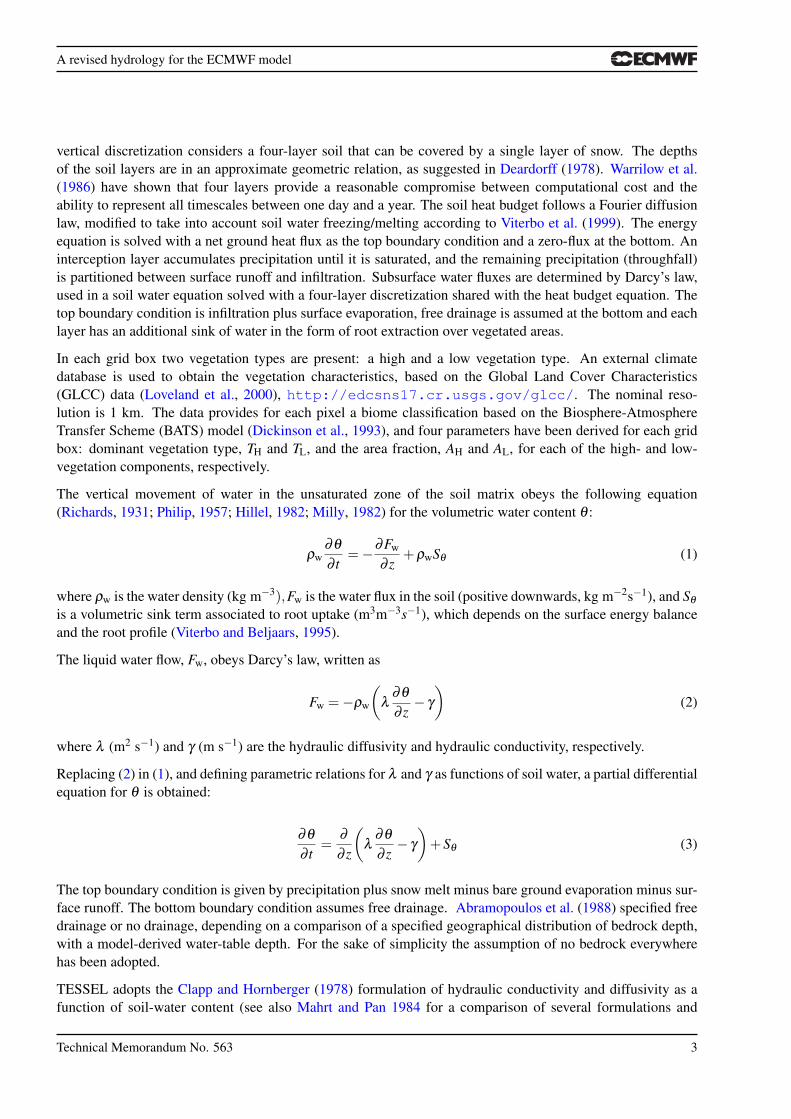
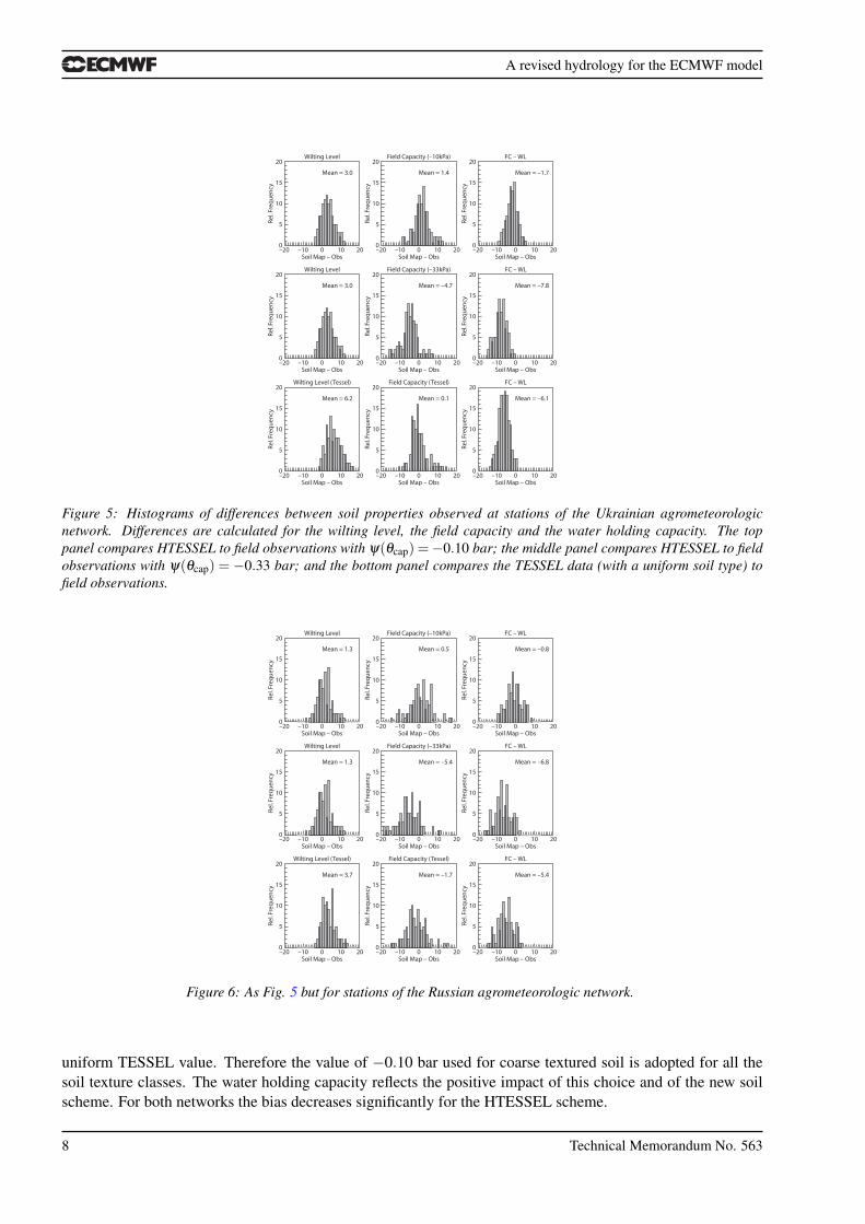
Figures 5 and 6 show the histogram of differences between the wilting level, the field capacity and the waterholding capacity (i.e. the difference between field capacity and wilting level) based on the field observationsat 20cm depth. The first panel (top) shows the histograms for the FAO soil texture derived values for the fieldcapacity calculated by setting ψ(θcap) = −0.10 bar (top panel). The second panel (middle) shows the samedata, but the field capacity was set to ψ(θcap) = −0.33 bar. The bottom panel shows the histograms for theuniform soil parameters used in the TESSEL scheme. The bias observed in the wilting point of the FAO soilmap is clearly substantially smaller than the bias of the uniform value used for the wilting point in TESSEL.For both networks the bias decreases by 50% or more when considering HTESSEL, with values 3.0 vol% and1.1 vol% for Ukraine and Russia respectively (for TESSEL the bias is 6.2 vol% and 3.4 vol%). For the fieldcapacity the results depend largely on the setting of ψ(θcap). Setting the value to−0.10 bar leads to differencessimilar to those observed for TESSEL. For the Ukrainian data the absolute bias slightly increases by 1.3 vol%;for Russia the absolute bias decreases by 1.2 vol%. Although Hillel (1982) indicate a matric potential ψ(θcap)of−0.33 bar as a common value for medium-textured soil field capacity, this leads in HTESSEL to a substantialdegradation when compared to the field capacity estimates. The bias increases to a high value of -4.7 vol% and-5.4 vol% for Ukraine and Russia respectively. These biases are significantly larger than those observed for the



Figure 5: Histograms of differences between soil properties observed at stations of the Ukrainian agrometeorologicnetwork. Differences are calculated for the wilting level, the field capacity and the water holding capacity. The toppanel compares HTESSEL to field observations with ψ(θcap) =−0.10 bar; the middle panel compares HTESSEL to fieldobservations with ψ(θcap) = −0.33 bar; and the bottom panel compares the TESSEL data (with a uniform soil type) tofield observations.

Figure 6: As Fig. 5 but for stations of the Russian agrometeorologic network.

uniform TESSEL value. Therefore the value of −0.10 bar used for coarse textured soil is adopted for all thesoil texture classes. The water holding capacity reflects the positive impact of this choice and of the new soilscheme. For both networks the bias decreases significantly for the HTESSEL scheme.



b. Soil moisture and fluxes

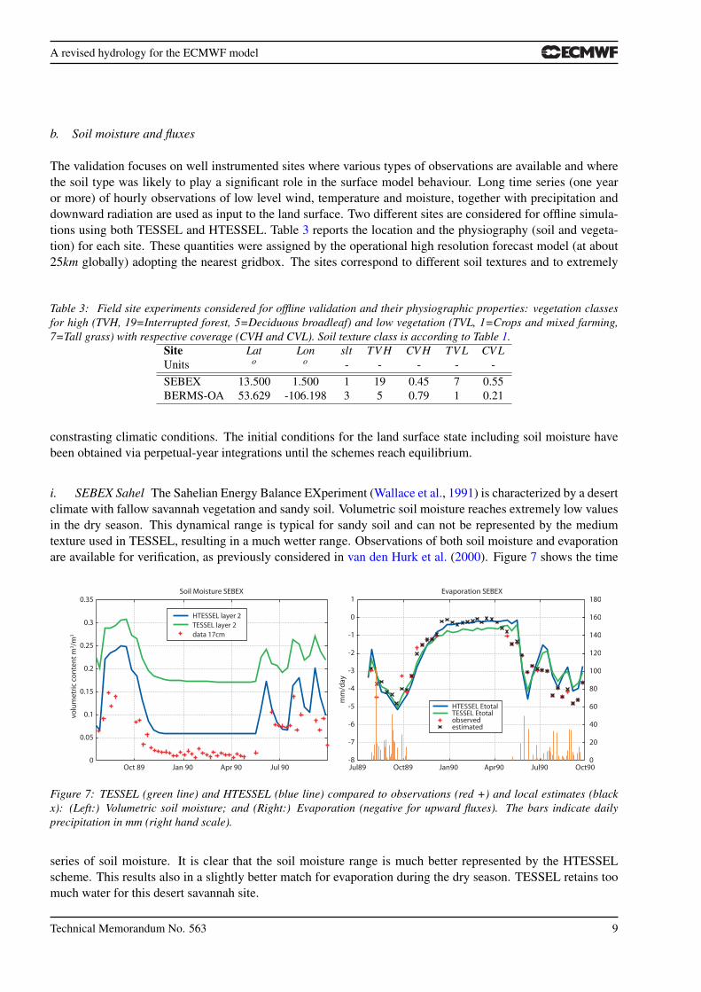
The validation focuses on well instrumented sites where various types of observations are available and wherethe soil type was likely to play a significant role in the surface model behaviour. Long time series (one yearor more) of hourly observations of low level wind, temperature and moisture, together with precipitation anddownward radiation are used as input to the land surface. Two different sites are considered for offline simula-tions using both TESSEL and HTESSEL. Table 3 reports the location and the physiography (soil and vegeta-tion) for each site. These quantities were assigned by the operational high resolution forecast model (at about25km globally) adopting the nearest gridbox. The sites correspond to different soil textures and to extremely

Table 3: Field site experiments considered for offline validation and their physiographic properties: vegetation classesfor high (TVH, 19=Interrupted forest, 5=Deciduous broadleaf) and low vegetation (TVL, 1=Crops and mixed farming,7=Tall grass) with respective coverage (CVH and CVL). Soil texture class is according to Table 1.

Site Lat Lon slt TV H CV H TV L CV LUnits o o - - - - -SEBEX 13.500 1.500 1 19 0.45 7 0.55BERMS-OA 53.629 -106.198 3 5 0.79 1 0.21

constrasting climatic conditions. The initial conditions for the land surface state including soil moisture havebeen obtained via perpetual-year integrations until the schemes reach equilibrium.

i. SEBEX Sahel The Sahelian Energy Balance EXperiment (Wallace et al., 1991) is characterized by a desertclimate with fallow savannah vegetation and sandy soil. Volumetric soil moisture reaches extremely low valuesin the dry season. This dynamical range is typical for sandy soil and can not be represented by the mediumtexture used in TESSEL, resulting in a much wetter range. Observations of both soil moisture and evaporationare available for verification, as previously considered in van den Hurk et al. (2000). Figure 7 shows the time

0

0.05

0.1

0.15

0.2

0.25

0.3

0.35

Oct 89 Jan 90 Apr 90 Jul 90

volu

met

ric

con

ten

t m

3 /m3

Soil Moisture SEBEX

-8

-7

-6

-5

-4

-3

-2

-1

0

1

Jul89 Oct89 Jan90 Apr90 Jul90 Oct900

20

40

60

80

100

120

140

160

180

mm

/day

Evaporation SEBEX

HTESSEL layer 2TESSEL layer 2data 17cm

HTESSEL EtotalTESSEL Etotalobservedestimated

Figure 7: TESSEL (green line) and HTESSEL (blue line) compared to observations (red +) and local estimates (blackx): (Left:) Volumetric soil moisture; and (Right:) Evaporation (negative for upward fluxes). The bars indicate dailyprecipitation in mm (right hand scale).

series of soil moisture. It is clear that the soil moisture range is much better represented by the HTESSELscheme. This results also in a slightly better match for evaporation during the dry season. TESSEL retains toomuch water for this desert savannah site.



ii. BERMS Boreal Forest The BERMS Old Aspen site located in Canadian Boreal forest (central Saskatchewan)has a high soil water retention. The data have been used for the validation of fluxes from ERA-40 in Betts et al.(2006). BERMS data represents one of the longest comprehensive time-series available for land surface modelverification. It has a marked interannual variability, allowing the evaluation of multiple time scales. Comparedto the SEBEX site, TESSEL soil texture (medium) properties are closer to HTESSEL (medium-fine, accordingto FAO). Still, both the absolute values and the interannual variability of soil moisture are better captured bythe HTESSEL as shown in Figure 8. This is explained by a more appropriate soil texture and by the increased

0

0.05

0.1

0.15

0.2

0.25

0.3

0.35

Jul 97 Jul 98 Jul 99 Jul 00 Jul 01 Jul 02 Jul 03 Jul 04

Soil Moisture BERMS-OA

volu

met

ric

con

ten

t m

3 /m3

HTESSEL 0-1mTESSEL 0-1m

data 0-1m

Figure 8: Volumetric soil moisture in TESSEL (green line) and HTESSEL (blue line) compared to observations (red +)for BERMS Old Aspen Boreal forest Canada.

memory in the Van Genuchten hydrology scheme. In fact according to Figure 2 , the conductivity is greatlyreduced for all the soil texture classes except coarse textured soils, leading to a much longer recharge/dischargeperiod.

4. Offline regional and global simulations

The verification of the models’ hydrology for large domains is a complex task. This is due both to the lackof direct observations and to a composite effect of shortcomings in land surface parametrizations, which pro-duce errors not easily traced to a single process. Global atmospheric re-analyses (ECMWF Re-Analysis se-ries, ERA15, ERA-40, ERA-Interim, National Centers for Environmental Predictions-Department of Energy,NCEP-DOE Reanalysis, Japanese Re-Analysis, JRA25) offer an estimate of water budgets on the global do-main. However, those estimates are heavily model-dependent and known to have deficiencies either in theland surface scheme or in the surface fluxes. This limits the validity for quantitative estimates. Seneviratneet al. (2004) and Hirschi et al. (2006a) bypassed the strong dependence on the land surface model formulationused in the reanalysis system by considering the water budget of large basins using both atmospheric moistureconvergence fields derived from reanalysis and observed river-discharge. Water balance closure can be thuscalculated without the use of atmospheric model precipitation and evaporation from the land surface model. ABasin Scale Water Budget (BSWB) dataset has been gathered for major World river catchments. Consideringhydrology over large domains allows the verification of subgrid-scale parameterizations (e.g. runoff) that cannot be evaluated at single instrumented sites, and the assessment of the overall behaviour of the scheme, whichmay be hidden in field site experiments (lack of representativity). We focus essentially on runoff and terrestrialwater storage changes to validate the performance of HTESSEL and TESSEL. Monthly time-scales are consid-ered for the largest catchments (mainly in the Northern hemisphere). Runoff at daily time-scales is evaluatedon a well-known catchment experiment, RhoneAgg (Boone et al., 2004).



a. The GSWP-2 experiment

The Global Soil Wetness Project, Second initiative, GSWP-2 (Dirmeyer et al., 1999, 2002; Gao et al., 2004)provides a set of near-surface forcing to drive land surface schemes offline. GSWP-2 covers the period July1982 to December 1995. The atmospheric forcing data are provided at a resolution of 1o globally on a domainof 360×150 grid-points and does not consider latitudes south of 60oS. The GSWP-2 data were originally basedon atmospheric reanalyses (NCEP-DOE Reanalysis) at 3-hour intervals, corrected using observational data asdetailed in (Dirmeyer et al., 2002). For the current experiments we have used the latest release of GSWP-2 atmospheric forcing based on ERA-40 where only precipitation is corrected using the Global PrecipitationClimatology Project (GPCP) dataset. These fields are labelled ERAGSWP. Temperature and pressure fields arerescaled according to elevation differences between the reanalysis model topography and that used in GSWP-2,while surface radiation and wind fields are unchanged. The state variables of surface pressure, air temperatureand specific humidity at 2m, as well as wind at 10m are provided as instantaneous values. The surface radiationand precipitation flux represent 3-hour averages. The GSWP-2 forcings are linearly interpolated in time to theintegration timestep of 30 minutes. The 10-year runs are aggregated into monthly climatologies and consideredover large catchments.

i. Terrestrial water storage The variation of the terrestrial water storage (TWS) can be expressed as:

dTWSdt

= P+E +R (12)

where P, E, R are the precipitation, evapotranspiration and runoff respectively. TWS accounts from both snow-pack and soil moisture variations. As previously mentioned, Eq. 12 can be combined with the atmosphericwater balance to eliminate the P and E terms which in atmospheric reanalysis are only indirectly constrainedby observations and strongly rely on model estimates. The expression obtained is

dTWSdt

=−dWdt−∇Q+R (13)

where the terms dWdt (atmospheric total column water variations), and −∇Q (atmospheric moisture conver-

gence), are taken from ERA-40 reanalysis and are thus directly constrained by assimilated observations (e.g.radiosondes). The runoff R is obtained by the observed river discharge from the Global Runoff Data Centre(GRDC) divided by the basin area.

The TWS estimates in the BSWB dataset, obtained from Eq. 13, are shown to correlate well with land surfacesoil moisture observations averaged on large domains. Moreover, mass variations detected from the GRACEsatellite mission correlate reasonably well with TWS (Hirschi et al., 2006b). In the GSWP-2 simulations, theTWS variations are computed directly from the monthly means of total column soil moisture variations and thesnow water equivalent variations. A number of Central European catchments are selected to show the effect ofthe revised hydrology. An improved description of the TWS change in HTESSEL-offline can be seen in Figure9, both when compared to ERA-40 (in which TESSEL is used in a coupled mode) and TESSEL-offline (drivenby ERAGSWP forcing). The reason for this improvement with respect to ERA-40 TWS is discussed in Section5.3. The slightly larger amplitude of TWS annual cycle in HTESSEL is mostly associated to the increasedwater holding capacity, as reported in Table 2.



1 2 3 4 5 6 7 8 9 10 11 12Time (months)

−3

−2

−1

0

1

2

3Te

rres

tria

l Sto

rag

e V

aria

tio

ns

[ mm

/d ]

TESSELHTESSELBSWB dataTESSEL (ERA−40)

FRACTION OF 1×1 GRID-BOX (central_europe) on Europe Domain0 - 0.1 0.1 - 0.2 0.2 - 0.3 0.3 - 0.5 0.5 - 0.7 0.7 - 0.9 0.9 - 1.01

Figure 9: Monthly Terrestrial Water Storage (TWS) changes (a) on Central European catchments (b): Wisla, Odra, Elbe,Weser, Rhine, Seine, Rhone, Po, North-Danube) for TESSEL (GSWP-2-driven, green line), HTESSEL (GSWP-2-driven,blue line), TESSEL in ERA-40 (black dashed line) and BSWB data (red diamonds) for 1986-1995.

-0.1 - 0.1

2.5 - 3

0.1 - 0.2

3 - 4

0.2 - 0.5

4 - 5

0.5 - 1

5 - 7

1 - 1.5

7 - 10

1.5 - 2

10 - 15

2 - 2.5

15 - 20

-0.1 - 0.1

2.5 - 3

0.1 - 0.2

3 - 4

0.2 - 0.5

4 - 5

0.5 - 1

5 - 7

1 - 1.5

7 - 10

1.5 - 2

10 - 15

2 - 2.5

15 - 20

Total Runoff [mm/day] (GRDC) on Globe Domain-0.1 - 0.1

2.5 - 3

0.1 - 0.2

3 - 4

0.2 - 0.5

4 - 5

0.5 - 1

5 - 7

1 - 1.5

7 - 10

1.5 - 2

10 - 15

2 - 2.5

15 - 20

Total Runoff [mm/day] (HTESSEL_GSWP2_1986_1995) on Globe Domain

Total Runoff [mm/day] (TESSEL_GSWP2_1986_1995) on Globe Domain

Figure 10: Total runoff from GRDC composite (top panel) HTESSEL (middle) and TESSEL (bottom) for the decade1986-1995



ii. Monthly runoff The Global Runoff Data Centre operates under the auspice of the World MeteorologicalOrganization and provides data for verification of atmospheric and hydrologic models. The GRDC databaseis updated continuously, and contains daily and monthly discharge data information for over 3000 hydrologicstations in river basins located in 143 countries. Over the GSWP-2 period the runoff data for 1352 dischargegauging stations were available. A 0.5o regular-grid mean annual runoff product is provided by the GRDC(http://www.grdc.sr.unh.edu/). This product is produced with an underlying precipitation climatology (Feketeet al., 2000), which is readjusted whenever the observed runoff exceeds the input precipitation. Given the largenumber of assumptions involved in the production of a global runoff climatology and particularly for precip-itation in ungauged basins, only a qualitative comparison is appropriate. Figure 10 shows the comparison ofHTESSEL and TESSEL with the GRDC product. Improvements are mainly visible in the Northern Hemi-sphere, where the non-zero runoff area is significantly increased in HTESSEL, consistent with GRDC. Thelimitations of ERA-GPCP precipitation dataset (used to force the stand-alone simulations) are clearly visible inthe tropical belt. In fact, a strong underestimation of rainfall (as reported in Betts et al. 2005 for Amazon basin)produces noticeable effects on the simulated annual runoff: both HTESSEL and TESSEL greatly underestimatethe GRDC runoff rates in this areas.

A basin-scale evaluation is considered as well. It is appropriate for large basins which are reasonably wellgauged and where the time-delay of the water path (routing) does not limit the validity of the comparison(e.g. excluding therefore the Amazon where the routing plays a major role in timing the runoff). Figure 11shows the errors of the monthly runoff evaluated on 41 different basins, listed in Table 4. RMSE and BIAS arecalculated on the (TESSEL and HTESSEL) monthly runoff against the GRDC monthly runoff estimates. The

1 3 5 7 9 11 13 15 17 19 21 23 25 27 29 31 33 35 37 39 41basin n.

0.0

0.2

0.4

0.6

0.8

1.0

1.2

1.4

1.6

1.8

2.0

Tot

al R

unof

f RM

SE

[ m

m/d

ay ]

1 3 5 7 9 11 13 15 17 19 21 23 25 27 29 31 33 35 37 39 41−1.3

−1.1

−0.9

−0.7

−0.5

−0.3

−0.1

0.1

0.3

0.5

Tot

al R

unof

f BIA

S [

mm

/day

]

Figure 11: Total runoff verification on basins against GRDC river discharge: BIAS (top) and RMSE (bottom). Shown areHTESSEL (black line) and TESSEL (grey shading).



Table 4: List of basins considered for the runoff verificationN. Basin N. Basin1 Ob 22 Volga2 Tura 23 Don3 Tom 24 Dnepr4 Podkamennaya-Tunguska 25 Neva5 Irtish 26 Baltic6 Amudarya 27 Elbe7 Amur 28 Odra8 Lena 29 Wisla9 Yenisei 30 Danube10 Syrdarya 31 Northeast-Europe11 Yukon 32 Po12 Mackenzie 33 Rhine13 Mississippi 34 Weser14 Ohio 35 Ebro15 Columbia 36 Garonne16 Missouri 37 Rhone17 Arkansas 38 Loire18 Xhangjiang 39 Seine19 Murray-darling 40 France20 Selenga 41 Central-Europe21 Vitim

HTESSEL simulation shows an overall reduction of the mean BIAS for most basins (with the Ohio river basin,n. 14 in Figure 11, being a noticable exception). For RMSE, roughly a third of the basins (N. 1-14) registera net deterioration, while the majority shows a marked improvement. This behaviour can be explained fromthe effect of snow ablation. The TESSEL snow treatment (not modified in HTESSEL scheme) suffers from thelack of a refreezing mechanism for water in the snow-pack, which activates the runoff too quickly and producesa pronounced peak.

Although the RMSE of the monthly runoff has deteriorated for snow-dominated basins, the BIAS is generallyreduced. The magnitude of the spring runoff peak is also in a better agreement with observations for HTESSELas shown in Figure 12 for the Yenisei Siberian basin (n. 9 in Figure 11). The correct timing will only beachieved by a revision of the snow scheme. The link between snow and soil moisture errors is discussed furtherin Section 5.3.



FRACTION OF 1x1 GRID-BOX (yenisei) on Globe Domain

0 - 0.1 0.1 - 0.2 0.2 - 0.3 0.3 - 0.5 0.5 - 0.7 0.7 - 0.9 0.9 - 1.01

−5

−4

−3

−2

−1

0

1

2

3

4

5

mm

/day

yenisei_HTESSEL

GPCP PrecipOffline Evap

ERA-40 POffline Runoff

ERA-40 EvapGRDC Runoff

yenisei_HTESSEL

Offline TWSBSWB TWS

1 2 3 4 5 6 7 8 1211109months

−5

−4

−3

−2

−1

0

1

2

3

4

5

mm

/day

1 2 3 4 5 6 7 8 1211109months

GPCP PrecipOffline Evap

ERA-40 POffline Runoff

ERA-40 EvapGRDC Runoff

Offline TWSBSWB TWS

1 2 3 4 5 6 7 8 1211109months

−5

−4

−3

−2

−1

0

1

2

3

4

5

mm

/day

1 2 3 4 5 6 7 8 1211109months

−5

−4

−3

−2

−1

0

1

2

3

4

5

mm

/day

yenisei_TESSEL yenisei_TESSEL

Figure 12: Yenisei water budget for HTESSEL and TESSEL during the GSWP-2 period (1986-1995) compared withBSWB, GRDC and ERA-40 estimates.



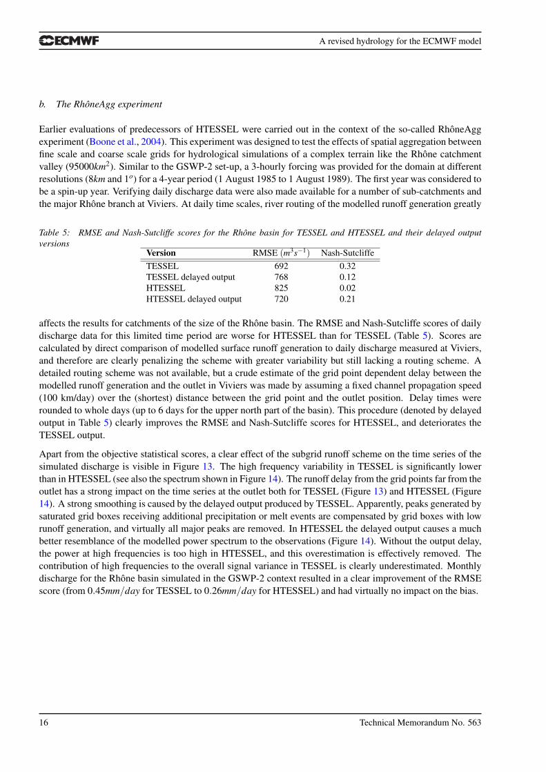
b. The RhoneAgg experiment

Earlier evaluations of predecessors of HTESSEL were carried out in the context of the so-called RhoneAggexperiment (Boone et al., 2004). This experiment was designed to test the effects of spatial aggregation betweenfine scale and coarse scale grids for hydrological simulations of a complex terrain like the Rhone catchmentvalley (95000km2). Similar to the GSWP-2 set-up, a 3-hourly forcing was provided for the domain at differentresolutions (8km and 1o) for a 4-year period (1 August 1985 to 1 August 1989). The first year was considered tobe a spin-up year. Verifying daily discharge data were also made available for a number of sub-catchments andthe major Rhone branch at Viviers. At daily time scales, river routing of the modelled runoff generation greatly

Table 5: RMSE and Nash-Sutcliffe scores for the Rhone basin for TESSEL and HTESSEL and their delayed outputversions

Version RMSE (m3s−1) Nash-SutcliffeTESSEL 692 0.32TESSEL delayed output 768 0.12HTESSEL 825 0.02HTESSEL delayed output 720 0.21

affects the results for catchments of the size of the Rhone basin. The RMSE and Nash-Sutcliffe scores of dailydischarge data for this limited time period are worse for HTESSEL than for TESSEL (Table 5). Scores arecalculated by direct comparison of modelled surface runoff generation to daily discharge measured at Viviers,and therefore are clearly penalizing the scheme with greater variability but still lacking a routing scheme. Adetailed routing scheme was not available, but a crude estimate of the grid point dependent delay between themodelled runoff generation and the outlet in Viviers was made by assuming a fixed channel propagation speed(100 km/day) over the (shortest) distance between the grid point and the outlet position. Delay times wererounded to whole days (up to 6 days for the upper north part of the basin). This procedure (denoted by delayedoutput in Table 5) clearly improves the RMSE and Nash-Sutcliffe scores for HTESSEL, and deteriorates theTESSEL output.

Apart from the objective statistical scores, a clear effect of the subgrid runoff scheme on the time series of thesimulated discharge is visible in Figure 13. The high frequency variability in TESSEL is significantly lowerthan in HTESSEL (see also the spectrum shown in Figure 14). The runoff delay from the grid points far from theoutlet has a strong impact on the time series at the outlet both for TESSEL (Figure 13) and HTESSEL (Figure14). A strong smoothing is caused by the delayed output produced by TESSEL. Apparently, peaks generated bysaturated grid boxes receiving additional precipitation or melt events are compensated by grid boxes with lowrunoff generation, and virtually all major peaks are removed. In HTESSEL the delayed output causes a muchbetter resemblance of the modelled power spectrum to the observations (Figure 14). Without the output delay,the power at high frequencies is too high in HTESSEL, and this overestimation is effectively removed. Thecontribution of high frequencies to the overall signal variance in TESSEL is clearly underestimated. Monthlydischarge for the Rhone basin simulated in the GSWP-2 context resulted in a clear improvement of the RMSEscore (from 0.45mm/day for TESSEL to 0.26mm/day for HTESSEL) and had virtually no impact on the bias.



0

1000

2000

3000

4000

5000

6000

7000

0786 1086 0187 0487 0787 1087 0188 0488 0788 1088 0189 0489 0789 1089

Dai

ly d

isch

arg

e (m

3 /s)

Date

Rhone at Viviers

obsHTESSEL (delayed)TESSEL (without delay)TESSEL (delayed)

Figure 13: Simulated and observed daily discharge at Viviers. Shown are model results for HTESSEL (with the delayedoutput being effective) and TESSEL both with and without the delayed output.

0.1

1

10

100

1000

10000

100000

1e+06

1e+07

0.001 0.01 0.1 1

Spec

tral

den

sity

Frequency [days^-1]

Rhone at Viviers

obsTESSELHTESSEL undelayedHTESSEL

Figure 14: Power spectrum of the observed and modelled daily discharge of the Rhone basin for the entire simulationperiod.



-1 -1

-1

1 -1

1

1

1

60°S

30°S

0°

30°N

60°N

135°W 90°W 45°W 0° 45°E 90°E 135°E

135°W 90°W 45°W 0° 45°E 90°E 135°E

135°W 90°W 45°W 0° 45°E 90°E 135°E

135°W 90°W 45°W 0° 45°E 90°E 135°E

Difference TESSEL – ERA40 global Mean err 0.065 rms 1.19

[K]

-13

-11

-9

-7

-5

-3

-1

1

3

5

7

60°S

30°S

0°

30°N

60°N

Difference HTESSEL – ERA40 global Mean err 0.0123 rms 1.08a) b)

c) d)

60°S

30°S

0°

30°N

60°N

Difference TESSEL – ERA40 global Mean err -0.362 rms 1.55

1

60°S

30°S

0°

30°N

60°N

Difference HTESSEL – ERA40 global Mean err -0.387 rms 1.52

Figure 15: Climate experiments, impact on 2m temperature (upper panels) and 2m dew point temperature (lower panels):(a, c) TESSEL, (b, d) HTESSEL. Shown are the mean 2m errors for JJA model climate evaluated against ERA-40.

5. Atmospheric-coupled simulations

Global atmospheric coupled experiments are used to evaluate the land-atmosphere feedback especially on near-surface atmospheric quantities. Various ensemble sets of multi-month integrations are performed. We refer tothese integrations as climate simulations. Short term predictions (12-hour) embedded in long data assimilationcycles (several months) are also used to evaluate the analysis increments, as a measure of model improvements.

a. Climate simulations

Two sets of climate simulations have been performed, using an atmospheric model configuration with 91 ver-tical layers and a grid-point resolution of about 120km (truncation T159 of a gaussian reduced grid). A 13-month 4-member ensemble for the period 01/08/2000 to 31/08/2001, and a multi-year 10-member ensemble of7-month runs (starting April 1 each year from 1991 to 1999) were executed. The experiments showed a verysmall atmospheric response to the land surface scheme modifications. A slightly positive impact is seen in tem-perature at 2m compared with ERA-40 climatology as shown in Figure 15. The 2m temperature RMSE erroris reduced from 1.19K to 1.08K, while the 2m dew-point temperature error is unchanged. The error patternsare similar for both 2m temperatures, and the error reduction in the HTESSEL simulation (Figure 15b and d) ismostly concentrated in Northern Hemisphere continental areas.

b. Extended Data Assimilation experiments

Considering the land surface water budget during a data assimilation cycle, Eq. 12 becomes

dTWSdt

= P+E +R+δA (14)



where δA represents the analysis increments (in snow δSn and soil moisture δθ ) added for each cycle of thedata assimilation system. It is assumed that a better land surface hydrology will lead to smaller systematicincrements δA. We compared the increments for two data assimilation cycles with TESSEL and HTESSEL asland surface schemes. For HTESSEL, the Optimum Interpolation (OI) soil moisture analysis (Mahfouf, 1991;Douville et al., 2000; Mahfouf et al., 2000) has also been revised for consistency. The OI coefficients have beenrescaled according to the ratio of water holding capacity in HTESSEL, a function of local soil texture, to theconstant value in TESSEL (see Table 2).

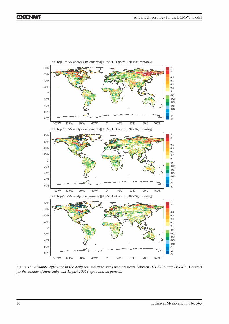
In order to focus on timescales relevant for the land-surface processes, we considered a 7-month period cover-ing the boreal summer (01/04/2006 to 31/10/2006). The analysis makes use of short-term forecast errors in 2mtemperature and relative humidity to correct soil moisture errors via a set of (OI) coefficients (see Douville et al.2000 for the detailed formulation). The absolute difference (HTESSEL - TESSEL) of the soil moisture analysisincrements over summer (JJA) is shown in Figure 16. Generally, a reduction of the mean daily soil moisture in-crements is observed at mid-latitudes, particularly over Europe and the central U.S. where the SYNOP networkis dense and the OI analysis most effective. This signal confirms the positive impact of HTESSEL over theseareas, certainly when we recall that the dynamical range of soil moisture is greatly increased. Northern regions,show larger SM analysis increments in HTESSEL for the month of June, associated with land surface spin-upfrom previous snow-cover, frozen soil conditions. Increments are mostly reduced in August (Figure 16c).

c. ERA-40 analysis increments and lesson learnt

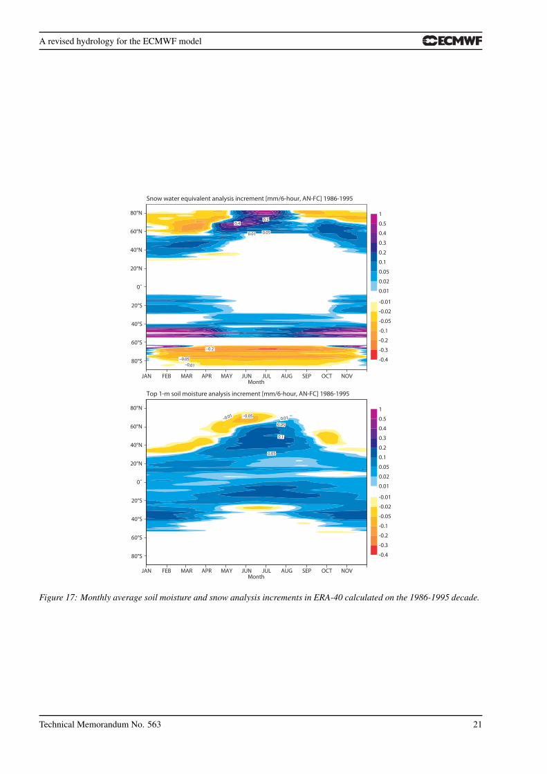
The long ERA-40 dataset with a frozen configuration of the data assimilation and modelling systems, providesthe opportunity to produce valuable diagnostics on data assimilation increments. It turns out that the soilmoisture and snow mass errors are tightly coupled at high latitudes. In ERA-40, the snow mass is analysedfrom SYNOP snow depth observations, with relaxation to climatology (12-day time scale) as a constraint indata-sparse areas. Systematic soil moisture/snow mass analysis increments indicate deficiencies in the system,which can be due to data or model errors, or due to a suboptimal data assimilation. Figure 17 shows the monthlymean data assimilation increments (expressed in mm/day) for snow and soil moisture, calculated from ERA-40and evaluated for the decade 1986-1995 (consistent with the GSWP-2 period). Results are presented in the formof a Hovmoller diagram (land-only zonal means as a function of latitude and month of the year). Focusing onnorthern latitudes, the snow analysis increments moving from 40oN in winter to 70− 80oN in June indicate apersistent positive correction which is attributed to the early melting of snow. This pattern is mirrored in thesoil moisture analysis which removes the water supply. The snow depth increments and the associated soilmoisture increments clearly suggest that the model is melting the snow too early, which is consistent with theoffline simulations as shown in Figure 12. In the latter case, the snow melt results in a runoff peak which is onemonth too early compared to the observations.

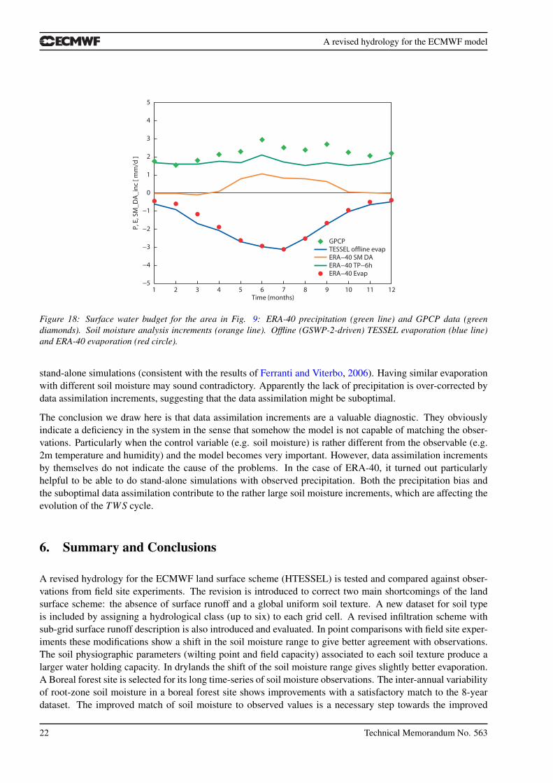
At mid-latitudes during the boreal summer months, positive soil moisture analysis increments are systematic(Figure 17), which suggests that the land surface model has a tendency of running dry in summer. From budgetdiagnostic on the European basins we know that the amplitude of the seasonal cycle of TWS-change in ERA-40is much smaller than observed (Figure 9). This is also concluded by Drusch and Viterbo (2007) by comparinganalysed soil moisture with in situ observations. More insight can be gained by considering, for the same basin,the water budget terms of Eq. 14 in stand-alone simulations with GSWP2 forcing and in ERA-40 (Figure 18).It is shown that much of the summer increments (up to 1 mm/day) in ERA-40 are a response to the precipitationdeficit in the short range forecasts of ERA-40 (also confirmed by van den Hurk et al., 2008). It is interestingthat both systems, i.e. ERA-40 affected by biased precipitation and with large data assimilation increments,and the stand-alone simulation with more realistic precipitation and no data assimilation, simulate very similarevaporation. Still the amplitude of the seasonal cycle of TWS is smaller in the ERA-40 system than in the



80°S

60°S

40°S

20°S

0°

20°N

40°N

60°N

80°N

160°W 120°W 80°W 40°W 0° 40°E 80°E 120°E 160°E

Diff. Top-1m-SM analysis increments [|HTESSEL|-|Control|, 200606, mm/day]

80°S

60°S

40°S

20°S

0°

20°N

40°N

60°N

80°N

160°W 120°W 80°W 40°W 0° 40°E 80°E 120°E 160°E

80°S

60°S

40°S

20°S

0°

20°N

40°N

60°N

80°N

160°W 120°W 80°W 40°W 0° 40°E 80°E 120°E 160°E



-5-2-1-0.8-0.5-0.3-0.2-0.1

0.10.20.30.50.8125

-5-2-1-0.8-0.5-0.3-0.2-0.1

0.10.20.30.50.8125

-5-2-1-0.8-0.5-0.3-0.2-0.1

0.10.20.30.50.8125

Figure 16: Absolute difference in the daily soil moisture analysis increments between HTESSEL and TESSEL (Control)for the months of June, July, and August 2006 (top to bottom panels).



Snow water equivalent analysis increment [mm/6-hour, AN-FC] 1986-1995

JANMonth

FEB MAR APR MAY JUN JUL AUG SEP OCT NOV

JANMonth

FEB MAR APR MAY JUN JUL AUG SEP OCT NOV

80°N

60°N

40°N

20°N

0˚

20°S

40°S

60°S

80°S

80°N

60°N

40°N

20°N

0˚

20°S

40°S

60°S

80°S

–0.01

–0.01

–0.2

–0.05

–0.05

Top 1-m soil moisture analysis increment [mm/6-hour, AN-FC] 1986-1995

-0.4

-0.3

-0.2

-0.1

-0.05

-0.02

-0.01

0.01

0.02

0.05

0.1

0.2

0.3

0.4

0.5

1

-0.4

-0.3

-0.2

-0.1

-0.05

-0.02

-0.01

0.01

0.02

0.05

0.1

0.2

0.3

0.4

0.5

1

0.01

0.05

0.05

0.1

0.01 0.05

0.20.4

Figure 17: Monthly average soil moisture and snow analysis increments in ERA-40 calculated on the 1986-1995 decade.



−5

−4

−3

−2

−1

0

1

2

3

4

5

P, E

, SM

_DA

_in

c [ m

m/d

]

GPCPTESSEL offline evapERA−40 SM DAERA−40 TP−6hERA−40 Evap

1 2 3 4 5 6 7 8 9 10 11 12Time (months)

Figure 18: Surface water budget for the area in Fig. 9: ERA-40 precipitation (green line) and GPCP data (greendiamonds). Soil moisture analysis increments (orange line). Offline (GSWP-2-driven) TESSEL evaporation (blue line)and ERA-40 evaporation (red circle).

stand-alone simulations (consistent with the results of Ferranti and Viterbo, 2006). Having similar evaporationwith different soil moisture may sound contradictory. Apparently the lack of precipitation is over-corrected bydata assimilation increments, suggesting that the data assimilation might be suboptimal.

The conclusion we draw here is that data assimilation increments are a valuable diagnostic. They obviouslyindicate a deficiency in the system in the sense that somehow the model is not capable of matching the obser-vations. Particularly when the control variable (e.g. soil moisture) is rather different from the observable (e.g.2m temperature and humidity) and the model becomes very important. However, data assimilation incrementsby themselves do not indicate the cause of the problems. In the case of ERA-40, it turned out particularlyhelpful to be able to do stand-alone simulations with observed precipitation. Both the precipitation bias andthe suboptimal data assimilation contribute to the rather large soil moisture increments, which are affecting theevolution of the TWS cycle.

6. Summary and Conclusions

A revised hydrology for the ECMWF land surface scheme (HTESSEL) is tested and compared against obser-vations from field site experiments. The revision is introduced to correct two main shortcomings of the landsurface scheme: the absence of surface runoff and a global uniform soil texture. A new dataset for soil typeis included by assigning a hydrological class (up to six) to each grid cell. A revised infiltration scheme withsub-grid surface runoff description is also introduced and evaluated. In point comparisons with field site exper-iments these modifications show a shift in the soil moisture range to give better agreement with observations.The soil physiographic parameters (wilting point and field capacity) associated to each soil texture produce alarger water holding capacity. In drylands the shift of the soil moisture range gives slightly better evaporation.A Boreal forest site is selected for its long time-series of soil moisture observations. The inter-annual variabilityof root-zone soil moisture in a boreal forest site shows improvements with a satisfactory match to the 8-yeardataset. The improved match of soil moisture to observed values is a necessary step towards the improved



assimilation of satellite data such as microwave radiances. In conclusion, the proposed changes to the ECMWFscheme address known short-comings without affecting the generally good performance of the land surfacemodel in providing the lower boundary conditions to the atmospheric model.

A set of regional stand-alone experiments (GSWP-2, 1986-1995) is used to evaluate the terrestrial water stor-age variations over the Central European river-basins in comparison with independent estimates based on at-mospheric moisture convergence data and river discharge observations. The model global annual runoff mapshows some small improvement when compared with the river discharge product. Quantitative evaluation ofthe runoff at monthly time-scales shows a net improvement of runoff timing in relevant catchments. In basinsdominated by snow, spring snow melt is still too early, because of errors in the snow scheme. The annual BIASin runoff is reduced for most of the basins considered. Errors in snow-melt are combined with a more activesurface runoff generation in HTESSEL, and therefore lead to increased RMSE in runoff. Daily time-scale forthe runoff are studied in the RhoneAgg experiment (1985-1989) where the main improvement is a spectrum ofriver discharge values closer to observations.

Atmospheric coupled verification is carried out using climate runs and long data assimilation experiments toevaluate the ensemble of changes in the land surface scheme and in the soil moisture analysis. At global scales,precipitation, snow and soil water errors are tightly coupled to water budget issues. Stand-alone integrationsallow one to separate errors in ERA-40 terrestrial water storage largely due to precipitation deficits in the 0-6hforecast (and to a suboptimal soil moisture correction) from snow related errors which remain a feature of thenew land surface scheme. The new soil hydrology appears to clearly benefit runoff and terrestrial water storagein snow-free areas. The operational implementation of a revised hydrology scheme is presented in Appendix.Future efforts to improve the annual terrestrial water balance will include adding a seasonal vegetation cycleand improving the snow scheme.

Acknowledgements

The authors wish to thank Adrian Tompkins, Thomas Jung, Paco Doblas-Reyes, Antje Weisheimer, for the helpwith climate runs, Matthias Drusch and Jean-Francois Mahfouf for discussions on the OI data assimilation.Emanuel Dutra and Patricia de Rosnay were helpful with independent evaluation of HTESSEL and valuablediscussions. Deborah Salmond, Mats Hamrud and Nils Wedi are thanked for help with IFS code, Jan Haselerand Joerg Urban for help with the scripts. Aaron Boone and Joel Noilhan are acknowledged for providingthe RhoneAgg dataset and for valuable discussions. We would like to thank the UK Centre for Ecology andHydrology, and the Fluxnet-Canada Research Network for making available the SEBEX and BERMS datasetsrespectively. Freddy Nachtergaele and Attila Nemes are acknowledged for help with soil texture data andvaluable discussions on soil properties aggregation. Alan Betts acknowledges support from NSF through grantATM-0529797. Rob Hine and Anabel Bowen are thanked for improving the figures appearance.



Appendix: Global scale implementation

The Integrated Forecast System (IFS) at ECMWF include the same land surface scheme which has to operateat various spatial resolutions, conserving the main features and most importantly the same water and energybudgets. Conservation of water storage when moving across resolution is a desirable property although noscheme can easily achieve this since averaging soil (as well as vegetation) properties lead to creation/destructionof information. As illustrated, the new parameterizations proposed for the soil hydrology consider a soil type(texture) which is used to assign hydrological properties and an orographic parameter which accounts for theterrain complexity.

The FAO/UNESCO Digital Soil Map of the World, DSMW (FAO, 2003) is available at the resolution of 5′×5′

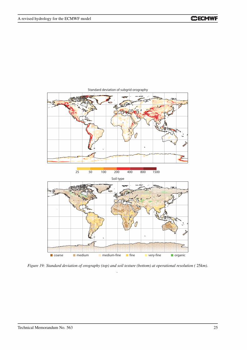
(about 10km). The FAO DSMW provides the information on two levels of soil depth 0−30cm and 30−100cm.The deep-soil layer (30−100cm) is used to prescribe the soil texture on the soil column. when moving acrossresolution. The orographic runoff parameter which determines the response of surface runoff to precipitationas a function of the complexity of the terrain uses the standard deviation of orography. This quantity is alreadyevaluated at high resolution and used in the turbulent orographic form drag (Beljaars et al., 2004). In Figure 19the soil texture map and the standard deviation of orography are reported for the 10-day forecast operationalresolution.

The soil texture and the standard deviation of orography are interpolated at various model resolutions. Thestandard deviation of orography can be interpolated bilinearly without special treatment. For the soil textureclass interpolation, the choice of a dominant soil texture aggregation is adopted since it largely preserves theoverall number of grid-points in each class. Thus water storage properties when moving across resolutions

Table 6: Percentage of soil texture class at T799 and T159 resolutions.Texture T 799 T 159Units % %Coarse 25.4 26.7Medium 38.7 40.2Medium-Fine 16.5 15.4Fine 16.5 15.3Very Fine 0.3 0.2Organic 2.6 2.2

is also preserved without creation of information. Sand and clay percentages, often used in place of texturalclasses, do not conserve hydraulic properties when moving across resolutions. Table 6 shows the percentage ofland points in each soil texture class at T159 (about 100km) and T799 (about 25km) resolution.

The adoption of a dominant soil texture permits an easy transition between TESSEL and HTESSEL soil mois-ture, which can be obtained by a linear rescale procedure taking into account field capacity and permanent wilt-ing point as detailed in http://www.ecmwf.int/products/changes/soil_hydrology_cy32r3/.The soil moisture rescale between TESSEL and HTESSEL is introduced to preserve atmospheric impact interms of evaporation.


http://www.ecmwf.int/products/changes/soil_hydrology_cy32r3/


Standard deviation of subgrid orography

25 50 100 200 400 800 1500

Soil type

coarse medium medium-fine fine very-fine organic

Figure 19: Standard deviation of orography (top) and soil texture (bottom) at operational resolution ( 25km)..



References

Abramopoulos, F., C. Rosenzweig, and B. Choudury, 1988: Improved ground hydrology calculations for globalclimate models (GCMs): Soil water movement and evapotranspiration. J. Climate, 1, 921–941.

Beljaars, A., P. Viterbo, M. Miller, and A. Betts, 1996: The anomalous rainfall over the United States duringJuly 1993: Sensitivity to land surface parameterization and soil moisture anomalies. Mon. Weather Rev., 124,362–382.

Beljaars, A. C. M., A. R. Brown, and N. Wood, 2004: A new parameterization of turbulent orographic formdrag. Q. J. R. Meteorol. Soc., 130, 1327–1347.

Betts, A. K., J. H. Ball, A. G. Barr, T. A. Black, J. H. McCaughey, and P. Viterbo, 2006: Assessing land-surface-atmosphere coupling in the ERA-40 reanalysis with boreal forest data. Agric. For. Meteorol., 140,365–382.

Betts, A. K., J. H. Ball, P. Viterbo, A. Dai, and J. Marengo, 2005: Hydrometeorology of the Amazon in ERA-40.J. Hydromet., 6, 764–774.

Boone, A., et al., 2004: The Rhone-aggregation land surface scheme intercomparison project: An overview. J.Climate, 17(1), 187–208.

Clapp, R. B. and G. M. Hornberger, 1978: Empirical equations for some soil hydraulic properties. WaterResources Res., 14, 601–604.

Cosby, B. J., G. M. Hornberger, R. B. Clapp, and T. Ginn, 1984: A statistical exploration of the relationshipsof soil moisture characteristics to the physical properties of soils. Water Resources Res., 20, 682–690.

Deardorff, J. W., 1978: Efficient prediction of ground surface temperature and moisture, with inclusion of alayer of vegetation. J. Geophys. Res., 83C, 1889–1903.

Dickinson, R., A. Henderson-Sellers, and P. Kennedy, 1993: Biosphere-atmosphere transfer scheme (BATS)version 1e as coupled to the NCAR community climate model. Technical Report NCAR/TN-387 + STR,NCAR Boulder, Colorado.

Dirmeyer, P., A. Dolman, and N. Sato, 1999: The pilot phase of the global soil wetness project. Bull. Am.Meteorol. Soc., 80, 851–878.

Dirmeyer, P., X. Gao, and T. Oki, 2002: The second global soil wetness project science and implementationplan. IGPO Int. GEWEX Project Office Publ. Series, 37, 75 pp.

Douville, H., P. Viterbo, J.-F. Mahfouf, and A. C. M. Beljaars, 2000: Evaluation of the optimum interpolationand nudging techniques for soil moisture analysis using FIFE data. Mon. Wea. Rev., 128, 1733–1756.

Drusch, M. and P. Viterbo, 2007: Assimilation of screen-level variables in ECMWF’s integrated forecast sys-tem: A study on the impact on the forecast quality and analysed soil moisture. Mon. Weather Rev., 135,300–314.

Dumenil, L. and E. Todini, 1992: A rainfall-runoff scheme for use in the hamburg climate model. Advancesin theoretical hydrology, A tribute to James Dooge. P. O’Kane, European Geophysical Society Series onHydrological Sciences 1, Elsevier, Amsterdam.

FAO, 2003: Digital soil map of the world (DSMW). Tech. rep., Food and Agriculture Organization of theUnited Nations. Re-issued version.



Fekete, B., C. Vorosmarty, and W. Grabs, 2000: Global, composite runoff fields based onobserved river discharge and simulated water balance. GRDC Report, available at htt p ://www.grdc.sr.unh.edu/html/paper/ReportA4.pd f .

Ferranti, L. and P. Viterbo, 2006: The European summer of 2003: Sensitivity to soil water initial conditions. J.Climate, 19, 3659–3680.

Gao, X., P. Dirmeyer, and T. Oki, 2004: Update on the second global soil wetness project (GSWP-2). GEWEXNewsletter, 14, 10.

Hillel, D., 1982: Introduction to Soil Physics. Academic Press.

Hirschi, M., S. Seneviratne, and C. Schar, 2006a: Seasonal variations in terrestrial water storage for majormid-latitude river basins. J. Hydromet., 7, 39–60.

Hirschi, M., P. Viterbo, and S. Seneviratne, 2006b: Basin-scale water-balance estimates of terrestrial waterstorage variations from ECMWF operational forecast analysis. Geophys. Res. Letters, 33, L21 401.

Jacquemin, B. and J. Noilhan, 1990: Sensitivity study and validation of a land-surface parameterization usingthe HAPEX-MOBILHY data set. Boundary-Layer Meteorol., 52, 93–134.

Koster, R. D., et al., 2004: Regions of strong coupling between soil moisture and precipitation. Science, 305,1138–1140.

Loveland, T. R., B. C. Reed, J. F. Brown, D. O. Ohlen, Z. Zhu, L. Youing, and J. W. Merchant, 2000: Devel-opment of a global land cover characteristics database and IGBP DISCover from the 1km AVHRR data. Int.J. Remote Sensing, 21, 1303–1330.

Mahfouf, J.-F., 1991: Analysis of soil moisture from near-surface parameters: A feasibility study. J. Appl.Meteorol., 30, 1534–1547.

Mahfouf, J.-F., P. Viterbo, H. Douville, A. Beljaars, and S. Saarinen, 2000: A revised land-surface analysisscheme in the integrated forecasting system. ECMWF Newsletter, 88, 8–13.

Mahrt, L. and H.-L. Pan, 1984: A two-layer model of soil hydrology. Boundary-Layer Meteorol., 29, 1–20.

Milly, P. C. D., 1982: Moisture and heat transport of hyseretic, inhomogeneous porous media: A matric head-based formulation and a numerical model. Water Resources Res., 18, 489–498.

Philip, J. R., 1957: Evaporation and moisture and heat fields in the soil. J. Meteorol., 14, 354–366.

Richards, L. A., 1931: Capillary conduction of liquids through porous mediums. Physics, 1, 318–333.

Robock, A., K. Y. Vinnikov, G. Srinivasan, J. K. Entin, S. E. Hollinger, N. A. Speranskaya, S. Liu, andA. Namkhai, 2000: The global soil moisture data bank. Bull. Am. Meteorol. Soc., 81, 1281–1299.

Seneviratne, S., P. Viterbo, D. Luthi, and C. Schar, 2004: Inferring changes in terrestrial water storage usingERA-40 reanalysis data: The Mississippi river basin. J. Climate, 17, 2039–2057.

Shao, Y. and P. Irannejad, 1999: On the choice of soil hydraulic models in land-surface schemes. Bound. LayerMeteor., 90, 83–115.

Uppala, S., et al., 2005: The ERA-40 re-analysis. Q. J. R. Meteorol. Soc., 131, 2961–3012.



van den Hurk, B., J. Ettema, and P. Viterbo, 2008: Analysis of soil moisture changes in Europe during a singlegrowing season in a new ECMWF soil moisture assimilation system. J. Hydromet., 9, 116–131.

van den Hurk, B. and P. Viterbo, 2003: The Torne-Kalix PILPS 2(e) experiment as a test bed for modificationsto the ECMWF land surface scheme. Global and Planetary Change, 38, 165–173.

van den Hurk, B., et al., 2005: Soil control on runoff response to climate change in regional climate modelsimulations. J. Climate, 18, 3536–3551.

van den Hurk, B. J. J. M., P. Viterbo, A. C. M. Beljaars, and A. K. Betts, 2000: Offline validation of the ERA-40surface scheme. ECMWF Tech. Memo. No. 295.

van Genuchten, M., 1980: A closed form equation for predicting the hydraulic conductivity of unsaturatedsoils. Soil Science Society of America Journal, 44, 892–898.

Viterbo, P. and A. C. M. Beljaars, 1995: An improved land surface parametrization scheme in the ECMWFmodel and its validation. J. Climate, 8, 2716–2748.

Viterbo, P., A. C. M. Beljaars, J.-F. Mahfouf, and J. Teixeira, 1999: The representation of soil moisture freezingand its impact on the stable boundary layer. Q. J. R. Meteorol. Soc., 125, 2401–2426.

Wallace, J. S., I. R. Wright, J. B. Stewart, and C. J. Holwill, 1991: The Sahelian Energy Balance EXperiment(SEBEX): ground based measurements and their potential for spatial extrapolation using satellite data. Adv.Space Res., 11, 31–41.

Warrilow, D. L., A. B. Sangster, and A. Slingo, 1986: Modelling of land-surface processes and their influenceon European climate. UK Met Office Report, Met O 20, Tech Note 38.


A revised hydrology for the ECMWF model: Verification from field ...

Documents