Imperial College Department of Physics MSc QFFF Dissertation A Review of the N =4 Super Yang-Mills/Type IIB AdS/CFT Correspondence Author: Peter Jones Supervisor: Professor Daniel Waldram Abstract The original AdS/CFT correspondence relating N =4 super Yang-Mills to Type IIB string theory in AdS 5 × S 5 is discussed. The necessary background is first reviewed, with the relevance to the conjecture emphasised throughout. The correspondence is then moti- vated via two arguments (the large N limit of gauge theories and the decoupling argument), and stated in three different forms of varying strength. A precise mapping between the observables of the two theories is then provided, and some simple checks of the weakest form of the correspondence (relating classical supergravity to strongly-coupled gauge theory) are discussed. Finally, extensions of the correspondence beyond the original case are briefly considered. Submitted in partial fulfilment of the requirements for the degree of Master of Science of Imperial College London. 20th September 2013

Welcome message from author
This document is posted to help you gain knowledge. Please leave a comment to let me know what you think about it! Share it to your friends and learn new things together.
Transcript

Imperial College Department of Physics
MSc QFFF Dissertation
A Review of the N=4 Super Yang-Mills/TypeIIB AdS/CFT Correspondence
Author:Peter Jones
Supervisor:Professor Daniel Waldram
Abstract
The original AdS/CFT correspondence relating N = 4 super Yang-Mills to Type IIBstring theory in AdS5 × S5 is discussed. The necessary background is first reviewed, withthe relevance to the conjecture emphasised throughout. The correspondence is then moti-vated via two arguments (the large N limit of gauge theories and the decoupling argument),and stated in three different forms of varying strength. A precise mapping between theobservables of the two theories is then provided, and some simple checks of the weakestform of the correspondence (relating classical supergravity to strongly-coupled gauge theory)are discussed. Finally, extensions of the correspondence beyond the original case are brieflyconsidered.
Submitted in partial fulfilment of the requirements for the degree of Master of Science ofImperial College London.
20th September 2013

Declaration
The following dissertation is my own work; the structure and manner in which concepts areexplained is my own, though numerous resources have been used in forming that understanding,and references are given where appropriate. Some sections follow closely the work of others, andare always indicated as such.
Acknowledgements
I would like to thank Professor Waldram for his help in supervising this dissertation, and for theuseful discussions we had regarding it.
2

Contents
Declaration 2
Acknowledgements 2
1 Introduction 5
I Ingredients of the Correspondence 7
2 Conformal Field Theory 82.1 Conformal Transformations . . . . . . . . . . . . . . . . . . . . . . . . . . . . . 82.2 The Conformal Algebra . . . . . . . . . . . . . . . . . . . . . . . . . . . . . . . 92.3 Aspects of Conformal Field Theory . . . . . . . . . . . . . . . . . . . . . . . . . 10
3 Supersymmetry and N = 4 Super Yang-Mills 143.1 The Super-Poincare Algebra and its Representations . . . . . . . . . . . . . . . . 143.2 The N = 4 Super Yang-Mills Theory . . . . . . . . . . . . . . . . . . . . . . . . 153.3 The Superconformal Group SU(2, 2|4) and its Representations . . . . . . . . . . 16
4 Superstrings and Supergravity 194.1 Review of the Bosonic String . . . . . . . . . . . . . . . . . . . . . . . . . . . . 194.2 Coupling the Bosonic String to a Background and Effective Spacetime Actions . 224.3 Superstrings and Type IIB Theory . . . . . . . . . . . . . . . . . . . . . . . . . 234.4 Branes in Supergravity and Superstring Theory . . . . . . . . . . . . . . . . . . 25
5 Anti-de Sitter Space 285.1 Definition of Anti-de Sitter Space . . . . . . . . . . . . . . . . . . . . . . . . . . 285.2 Coordinate Systems on AdSd . . . . . . . . . . . . . . . . . . . . . . . . . . . . 295.3 The Conformal Boundary of AdSd . . . . . . . . . . . . . . . . . . . . . . . . . 305.4 Poincare Coordinates . . . . . . . . . . . . . . . . . . . . . . . . . . . . . . . . 31
II The N = 4 SYM/Type IIB AdS/CFT Correspondence 32
6 Motivating the AdS/CFT Correspondence 336.1 Motivation: The Large N Limit of Gauge Theories . . . . . . . . . . . . . . . . 336.2 Motivation: The Decoupling Argument . . . . . . . . . . . . . . . . . . . . . . . 366.3 Statement of the Correspondence . . . . . . . . . . . . . . . . . . . . . . . . . . 386.4 First Check: Correspondence of the Global Symmetries . . . . . . . . . . . . . . 39
7 The Field/Operator Map and the Witten Prescription 40
3

CONTENTS 4
7.1 The Field/Operator Map . . . . . . . . . . . . . . . . . . . . . . . . . . . . . . 407.2 The Witten Prescription for Mapping Correlators . . . . . . . . . . . . . . . . . 427.3 Example: Calculation of the 2-point Function for Scalars . . . . . . . . . . . . . 437.4 Example: The 3-point Function for the R-Symmetry Currents and its Anomaly . 45
III Conclusion: Beyond the Original Conjecture 49
8 Conclusion 508.1 Extensions of the Correspondence . . . . . . . . . . . . . . . . . . . . . . . . . . 508.2 Closing Remarks . . . . . . . . . . . . . . . . . . . . . . . . . . . . . . . . . . . 51
References 52

Chapter 1
Introduction
The Anti-de Sitter/Conformal Field Theory (AdS/CFT) correspondence, otherwise known as thegauge/gravity duality, is one of the major breakthroughs to arise from string theory in recentyears. The correspondence is significant from both a conceptual and practical point of view;not only does it shed valuable physical insight into both sides of the correspondence, but it alsoprovides new ways of performing calculations where more conventional methods are intractable.
The correspondence, roughly speaking, states the equivalence between a string theory con-taining gravity living in a certain geometry, and a gauge theory living on the boundary of thatgeometry. More precisely, the strongest form of the original correspondence due to Maldacena[MAL] states that the 10-dimensional Type IIB superstring theory on the product space AdS5×S5
(with 5-form flux N) is equivalent to N = 4 super Yang-Mills (SYM) theory with gauge groupSU(N), living on the flat 4-dimensional boundary of AdS5. What one means by ‘equivalence’ inthis context is something that will be clarified throughout this dissertation; essentially it meansthat there is a one-to-one correspondence between all aspects of the theories including the globalsymmetries, observables, and correlation functions. The theories are thus considered to be dualdescriptions of each other; this notion of duality is an interesting one because it turns out thatthe regimes within which it is possible to perform calculations easily do not coincide on thetwo sides of the correspondence. Indeed, the correspondence comes in several forms of differentstrengths, related to which restrictions are imposed on the various parameters in the theories;depending on the form of the correspondence, calculations on either side are possible to differingextents. No form of the correspondence has been proven in a rigorous manner (leading it to beknown also as the AdS/CFT conjecture), though considerable evidence has been offered in theirsupport, some of which we shall discuss in the present dissertation.
As we shall see, the correspondence can be motivated by an argument which itself restsfundamentally on a duality; namely, a dual interpretation of objects in string theory known asD-branes. On the one hand, these objects are considered to be dynamical hyperplanes uponwhich the endpoints of open strings are fixed (but are free to move parallel to the brane); suchobjects arise naturally in the analysis of the open string as we shall see. On the other hand,D-branes can be considered as background solutions (with particular symmetries) to the lowenergy effective spacetime theory of string theory known as supergravity ; one can then considerclosed strings propagating in such a background. That these points of view are equivalent is ofgreat importance, since by considering a particular physical set-up from each in turn, we shall seethat (in certain limits) there are two decoupled theories in both interpretations; by recognising acommon theory present, we are then led to identify the other two theories as equivalent or dualdescriptions, which is exactly the AdS/CFT correspondence mentioned above. This decouplingargument will be described in detail in chapter 6.
The fact that the information of the 10-dimensional dynamics (compactified onto a 5-dimensional space) can somehow be encoded in a 4-dimensional theory has led to the conjecturebeing known as the holographic principle, in analogy to the way in which conventional hologramsencode the information about a 3-dimensional object in a 2-dimensional surface. Indeed, thequestion of whether holography may play a role in a theory of quantum gravity has been enter-
5

CHAPTER 1. INTRODUCTION 6
tained for sometime, originating in the crucial result that black holes have an entropy proportionalto the area of their horizon [BEK]; this is in contrast to familiar thermodynamic systems for whichthe entropy is an extensive property that scales with the volume of the system. Since the originalMaldacena conjecture the AdS/CFT correspondence has been extended to other cases, contain-ing, for example, field theories with less supersymmetry or no conformal symmetry on the gaugeside, and different string theories and geometries on the gravity side; in all cases there remainsthis holographic aspect, equating two theories in spacetimes of different dimensions. Further-more, recently there has been considerable work into investigating a possible de Sitter/ConformalField Theory (dS/CFT) correspondence [STR], something that would perhaps attract even moreinterest considering the positiveness of the experimentally observed cosmological constant.
In addition to these conceptual curiosities, the correspondence is computationally very pow-erful by virtue of the fact that non-perturbative problems in super Yang-Mills theory can bestudied using perturbative string theory. In fact, in certain limits (to be discussed in more de-tail later) Type IIB string theory reduces to a classical supergravity theory, and so one mayuse the correspondence to study strongly-coupled gauge theories simply using classical gravitytheory. Although the gauge theories in question (e.g. N = 4 SYM with a large number ofcolours N) are quite remote from those we believe to be realised in nature (e.g. QCD whichis neither supersymmetric nor conformal and has N = 3), the correspondence is continuallybeing extended to new cases, and valuable general properties of strongly-coupled gauge theoriesare being learnt from these studies. The correspondence has also recently been greatly usedin the field of condensed matter physics, and has led to the creation of a subject now knownas the Anti-de Sitter/Condensed Matter Theory (AdS/CMT) correspondence (see [HAR]). Weshall not discuss such applications in the present dissertation however, and our focus shall bepredominantly on the original Maldacena correspondence; it is nevertheless interesting to notethat a correspondence that appears so fundamental has found application to the physics of largesystems.
The AdS/CFT correspondence brings together many areas of modern theoretical physics. Forexample, on one side of the correspondence one has the N = 4 SYM theory; this is a supersym-metric but also a conformal field theory, which in fact combine to form a larger superconformalsymmetry. On the other side of the correspondence one must study superstring and supergravitytheory (including the properties of D-branes), in addition to the properties of a maximally sym-metric spacetime known as anti-de Sitter space. In Part 1 of this dissertation I will thus introducethe different components of the correspondence, all of which must be adequately tackled in orderto understand the conjecture; considerable time will thus be devoted to this purpose, and therelevance to the correspondence will be emphasised throughout. In Part 2 I will then motivate(via two arguments) and state the original AdS/CFT conjecture in its different forms; I will thendescribe the precise mapping between the observables on the two sides, and perform some simplechecks of the correspondence. Finally, in Part 3 I will briefly describe some extensions of thecorrespondence to cases other than the original Maldacena conjecture.

Part I
Ingredients of the Correspondence
7

Chapter 2
Conformal Field Theory
The study of conformal field theory (CFT) will be crucial in the following since, in addition tothe fact that string theory can be described as a 2-dimensional CFT, the gauge theory in thecorrespondence (N = 4 SYM) exhibits conformal invariance. A CFT is simply a quantum fieldtheory (QFT) that has conformal invariance; however, this turns out to be a very strict condition,greatly restricting the QFT and its correlation functions, and requiring the introduction of newconcepts not present in other field theories. In this chapter we will first introduce conformaltransformations and the conformal algebra, and then proceed to review the key features of CFTrelevant for the AdS/CFT correspondence.
2.1 Conformal Transformations
A conformal transformation in R1,d−1 is a local transformation xµ → xµ(x) such that the lineelement changes by a scaling:
ηµνdxµdxν = Ω(x)2ηρσdx
ρdxσ (2.1)
for some function Ω(x) i.e. angles, but not necessarily distances, are preserved by the transfor-mation. From the chain rule dxµ = (∂xµ/∂xσ)dxσ one then trivially derives:
ηµν∂xµ
∂xσ∂xν
∂xρ= Ω(x)2ηρσ (2.2)
and we see clearly that Poincare transformations, for which Ω(x) = 1 (forming the isometrygroup of R1,d−1), are a subset of conformal transformations. By considering infinitesimal trans-formations of the form xµ = xµ + vµ(x) and Ω(x) = 1 +ω(x) it is easy to derive from (2.2), byworking to first order in vµ and ω, the equation:
∂µvν + ∂νvµ = 2ω(x)ηµν (2.3)
Taking the trace one finds that ω(x) = (∂ · v(x))/d and thus we obtain the conformal Killingequation:
∂µvν + ∂νvµ =2
d(∂ · v)ηµν (2.4)
Note that in a general spacetime this equation changes by replacing ηµν → gµν and ∂ → ∇,though our case of interest will be that of flat spacetime above.
One must solve (2.4) for v(x) to obtain the infinitesimal conformal transformations. Ford = 2, it is very easy to show by considering the different possible values of µ and ν that equation(2.4) is equivalent to the Cauchy-Riemann equations, and thus conformal transformations aregenerated by all holomorphic functions v(x) ≡ v1(x) + iv2(x). For d > 2 the general solution to(2.4) is (see [GOM]):
vµ(x) = aµ + ωµνxν + λxµ + bµx
2 − 2(b · x)xµ (2.5)
8

CHAPTER 2. CONFORMAL FIELD THEORY 9
where ωµν = −ωνµ but aµ, bµ and λ are arbitrary. The parameters aµ, ωµν , λ and bµ correspondto translations, rotations, scale transformations (or dilatations), and special conformal transfor-mations respectively, giving a total of d+ d(d− 1)/2 + 1 + d = (d+ 1)(d+ 2)/2 parameters.
In addition to the above continuous transformations generated by infinitesimal Killing vectors,one can consider a discrete conformal transformation, known as inversion, defined by:
xµ → xµ = xµ/x2 (2.6)
which is clearly a conformal transformation with Ω(x) = 1/x2. Note that the term ‘conformaltransformations’ usually refers to the continuous transformations generated by infinitesimal con-formal Killing vectors as in (2.5) and so does not include inversions (much in the same way thatthe term ‘Lorentz transformations’ usually only refers to the proper (orthochronous) subgroup ofthe Lorentz group). Importantly, the special conformal transformations can be constructed byperforming a translation, preceded and proceeded by an inversion:
xµ → xµ
x2→ xµ
x2+bµ →
xµ
x2 + bµ
(xµ
x2 + bµ)2=
xµ + bµx2
1 + b2x2 + 2b · x=bµ→0 xµ+(bµx2−2 (b · x)xµ) (2.7)
which is exactly the infinitesimal form of a special conformal transformation as contained withinequation (2.5).
2.2 The Conformal Algebra
The conformal transformations form a group known as the conformal group. Denoting thegenerators of translations, rotations, scale transformations, and special conformal transformationsrespectively as Pµ,Mµν , D and Kµ, we may use the infinitesimal transformations contained in(2.5) to easily find the following differential operator representations:
Pµ ≡ −i∂µ (2.8)
Mµν ≡ −i(xµ∂ν − xν∂µ) (2.9)
D ≡ ixµ∂µ (2.10)
Kµ ≡ −i(x2∂µ − 2xµx · ∂) (2.11)
We can then easily calculate the commutators, giving the conformal algebra as [GOM]:
[Kµ, Pν ] = 2i(ηµνD +Mµν) (2.12)
[Mµν , Pρ] = i(ηµρPν − ηνρPµ) (2.13)
[Mµν ,Kρ] = i(ηµρKν − ηνρKµ) (2.14)
[D,Pµ] = −iPµ (2.15)
[D,Kµ] = iKµ (2.16)
[Mµν , D] = 0 (2.17)
[Pµ, Pν ] = [Kµ,Kν ] = 0 (2.18)
[Mµν ,Mρσ] = i (ηµρMνσ − ηµσMνρ + ηνσMµρ − ηνρMµσ) (2.19)
There are several interesting observations to make regarding this algebra. First, the Poincarealgebra is clearly contained within it (in (2.13), (2.18) and (2.19)), as expected. Second, equa-tion (2.14) states that Kµ is a Lorentz vector, whilst (2.17) states that D is a Lorentz scalar.Third, equation (2.12) shows that dilatations may be obtained simply from combining Poincare

CHAPTER 2. CONFORMAL FIELD THEORY 10
transformations and special conformal transformations (and thus the entire conformal algebracan be generated by Poincare transformations and inversion alone, following the discussion atthe end of section 2.1). Finally, equations (2.15)-(2.16) show that Pµ and Kµ are raising andlowering operators respectively for the dilatation operator D, which proceeds in direct analogywith the algebra for the harmonic oscillator (and which we discuss further in section 2.3). Onecan also interpret D as reading off the length dimension (not to be confused with its inverse,the mass dimension) of the other operators (as is appropriate for a scaling operator) from (2.15-2.17), since Pµ,Kµ and Mµν have length dimensions −1,+1 and 0 respectively, as is clear from(2.8)-(2.11).
The algebra above turns out to be isomorphic to SO(2, d) (including inversions one in fact hasthe full orthogonal group O(2, d)), the dimension of which agrees with the number of parameterscalculated in section 2.1. This can be seen more explicitly by defining antisymmetric generatorsLMN (M = 0, 1...d + 1) as the following linear combinations of conformal generators (see[GOM]):
Lµν ≡Mµν Ld,d+1 ≡ D Lµd ≡1
2(Pµ +Kµ) Lµ,d+1 ≡
1
2(Pµ −Kµ) (2.20)
where µ = 0, 1, ...d− 1. Using the conformal algebra, one can then straightforwardly show thatthe generators LMN do indeed satisfy the SO(2, d) algebra. This will be important later in theAdS/CFT correspondence, where we shall see an identification between the conformal group in4-dimensions and the isometry group of AdS5 (see section 6.4).
2.3 Aspects of Conformal Field Theory
One of the central premises of relativistic quantum field theory is that the field operators transformunder a representation of the Poincare group. Under a Poincare group transformation x→ x =g · x, a field operator φA(x) transforms as (following [GOM]):
φA(x)→ φA(x) = RAB(g)φB(x) (2.21)
or equivalently:φA(x) = RAB(g)φB(g−1 · x) (2.22)
where RAB(g) is a representation of the group element g (for example, RAB(g) = 1 for all g fora scalar field). We see that in addition to the transformation of the field argument, there isadditional information specified about how the internal or ‘spin’ index A of the field transforms;this additional information is only relevant for Lorentz transformations, as the translations actonly on the argument of the field. For a conformal field theory, one must specify one further bitof information, namely how a field operator transforms under a scale transformation. Under adilatation x→ x = λx we have:
φA∆(x) = λ−∆φA∆(λ−1x) (2.23)
where ∆ is known as the dimension of the operator φ∆. The dimension of φA∆ can be definedequivalently as:
[D,φA∆] = −i∆φA∆ (2.24)
i.e. as an eigenvalue of the dilatation operator.We define in general a primary operator [GOM] to be one that transforms as a tensor density
under general conformal transformations. For example, a scalar φ(x) transforms as:
φ(x) =
∣∣∣∣∂x∂x∣∣∣∣∆/d φ(g−1 · x) (2.25)

CHAPTER 2. CONFORMAL FIELD THEORY 11
The descendants are then obtained from the primaries by taking derivatives; these do not trans-form as tensor densities and so cannot be primaries. These concepts can also be introduced in analternative way. We mentioned previously that Pµ and Kµ act as raising and lowering operatorsfor the dilatation operator D. We can see this by considering an operator φ∆ of dimension ∆and finding the dimension of [Pµ, φ∆]. Using the Jacobi identity we have;
[D, [Pµ, φ∆]] = −[Pµ, [φ∆, D]]− [φ∆, [D,Pµ]] (2.26)
and thus using the conformal algebra we find:
[D, [Pµ, φ∆]] = −i(∆ + 1)[Pµ, φ∆] (2.27)
showing that [Pµ, φ∆] has dimension ∆ + 1 as claimed. An analogous proof shows that [Kµ, φ∆]has dimension ∆ − 1. For a representation to be unitary the conformal dimensions must bepositive, and thus there must be an operator in the representation of lowest dimension (i.e.that is annihilated by Kµ), since otherwise one can continuously generate lower-dimensionaloperators. These lowest-dimensional operators are the primary operators, now defined by thecondition [Kµ, φ
A] = 0. A unitary representation of the conformal group is then given by asingle primary operator φA, together with the set of descendants of this primary which areobtained by application of the translation generator Pµ. We will see a generalisation of thisstructure when we consider the superconformal algebra in section 3.3.
There is an important result that one can derive immediately for field theories that have(classical) conformal invariance. Noether’s theorem proves the existence and provides the con-struction of a conserved current for every continuous symmetry of the action. In the case ofPoincare invariance, one obtains the familiar currents given by the energy-momentum tensor Tµν
as (see [ERD]):jµ ≡ Tµνvν (2.28)
where vν is a Killing vector generating Lorentz transformations or translations, and the currentsare conserved in the sense that ∂µj
µ = 0. From translation and Lorentz symmetry respectivelyone finds the conditions ∂µT
µν = 0 and Tµν = Tνµ (sometimes after requiring ‘improvement’ ofthe energy-momentum tensor). Interestingly, it is possible to show that the currents that arisedue to full conformal invariance have the same form as in (2.28), where now vµ can represent ageneral conformal Killing vector. Conformal invariance means that the associated current shouldbe conserved and so we find:
∂µjµ = 0 = ∂µT
µνvν + Tµν∂µvν = Tµν1
2(∂µvν + ∂νvµ) (2.29)
where in the last equality we used the conservation and symmetry of Tµν , and thus using theconformal Killing equation (2.4) we find:
0 = Tµν1
2
2
dηµν∂ · v = Tµµ
∂ · vd
(2.30)
which implies that the energy-momentum tensor is traceless i.e. Tµµ = 0. Classically, a field theoryis conformally invariant if there are no dimensionful couplings in the action (e.g. mass terms); thisis intuitive, since a dimensionful coupling sets a scale, thereby breaking scale invariance. Uponquantization however, conformal invariance may be broken in the form of anomalies arising fromloop corrections. The form of these anomalies is sometimes in the non-vanishing expectationvalue of Tµµ , conflicting with the classical conformal invariance condition we derived in (2.30). In

CHAPTER 2. CONFORMAL FIELD THEORY 12
fact, a necessary condition for a theory to be conformally invariant quantum mechanically (see[GOM] for a discussion) is the vanishing of the renormalisation-group beta functions [PES]:
βg(µs) ≡ µs∂g
∂µs(2.31)
where g is a coupling in the theory and µs is the renormalisation scale, since this quantity directlymeasures the scale-dependence of the couplings in the theory. This fact will be very importantin chapter 4 when we discuss the effective spacetime actions for string theories.
The key observables that one wants to calculate in any quantum field theory are the n-pointcorrelation functions. Conformal invariance turns out to provide very strict conditions on theforms of the n-point functions (for small values of n). The statement of conformal invariance forthe n-point correlation function of primary operators θAii (from which one can derive correlationfunctions involving descendants) is:
〈θA11 (x1)...θAnn (xn)〉 = 〈θA1
1 (x1)...θAnn (xn)〉 (2.32)
where θAii are the transformed operators. We shall illustrate the power of the restrictions thatconformal invariance imposes for the simplest case of scalar primary operators, following [GOM].
• Consider the 1-point function of a scalar primary operator of dimension ∆. Translationinvariance clearly fixes:
〈θ∆(x)〉 = C (2.33)
for a constant C. Scale invariance under dilatations x = λx then imposes 〈θ∆(x)〉 =〈θ∆(x)〉 from (2.32), and since θ∆(x) = λ−∆θ∆(x) (from (2.23)) we have C = λ−∆C,which forces C and thus the 1-point function to zero unless ∆ = 0 in which case theoperator is the identity. We thus have the result:
〈θ∆(x)〉 = δ∆,0 (2.34)
• A less trivial example is given by the 2-point function. Recall that in general quantumfield theories the 2-point functions can be very complicated, and are usually only accessiblevia the machinery of perturbation theory. Here we shall see that their form is entirelydetermined by conformal invariance. By translation and Lorentz invariance we see that the2-point function of scalar primary operators must take the form:
〈θ∆1(x1)θ∆2(x2)〉 = f(|x1 − x2|) (2.35)
for some function f(x). Scale invariance then fixes 〈θ∆1(x1)θ∆2(x2)〉 = 〈θ∆1(x1)θ∆2(x2)〉and thus using (2.35) together with x = λx and θ∆(x) = λ−∆θ∆(x) we have:
f(λ|x1 − x2|) = λ−(∆1+∆2)f(|x1 − x2|) (2.36)
from which one can inspect the solution:
f(|x1 − x2|) =C
|x1 − x2|∆1+∆2(2.37)
for some constant C. We are not quite finished however, since we must still imposeinvariance under special conformal transformations. Given the discussion at the end ofsection 2.1, it is much easier to achieve this by instead imposing invariance under inversion.

CHAPTER 2. CONFORMAL FIELD THEORY 13
Under inversion xµ = xµ/x2 we have θ∆(x) = θ∆(x)/(x2∆) and thus using (2.32) and(2.37) we see that inversion invariance imposes:
1
|x1 − x2|∆1+∆2=
1
x2∆11
1
x2∆22
1
|x1 − x2|∆1+∆2(2.38)
Using the definition of inversion xµ = xµ/x2, straightforward algebra shows that:
x21x
22
|x1 − x2|2=
1
|x1 − x2|2(2.39)
and thus combining this with (2.38) we obtain the equality:
x2∆11 x2∆2
2
|x1 − x2|∆1+∆2=
[x2
1x22
|x1 − x2|2
]∆1+∆22
(2.40)
from which we can infer the condition ∆1 = ∆2. The form of the 2-point function is thusfixed as:
〈θ∆1(x1)θ∆2(x2)〉 =Cδ∆1,∆2
|x1 − x2|2∆1(2.41)
for some constant C (which can be set to 1 with appropriate field redefinition). We seethat the 2-point functions in a conformal field theory are thus entirely determined by thespectrum ∆.
• One can proceed in a similar fashion to the 2-point function above to see what conditionsconformal invariance places on higher-point functions. We shall not repeat the analysishere, but we state that the 3-point function of scalar primary operators is restricted to takethe form:
〈θ∆1(x1)θ∆2(x2)θ∆3(x3)〉 =C
|x1 − x2|∆1+∆2−∆3 |x1 − x3|∆1+∆3−∆2 |x2 − x3|∆2+∆3−∆1
(2.42)where C is a constant that, unlike the 2-point function case, cannot be removed by fieldredefinition and is in fact theory-dependent. We see that, although the overall normalisationis not, the spacetime dependence of the 3-point function is still entirely fixed by conformalinvariance.
• For n-point functions with n ≥ 4 the spacetime dependence is no longer entirely fixedeither. This is due to the existence of conformally invariant cross-ratios of coordinateswhich the correlation function can thus depend on arbitrarily. We shall not need to discussn-point functions with n ≥ 4 any further in the following however.
Although the above analysis was for scalar primary operators, similar results follow through forhigher-rank tensor operators. For example, the 2-point function of two vector primary operatorscan be derived in an analogous (and only slightly more complicated) way to the scalar case andis given by (see [GOM]):
〈V µ∆1
(x1)V ν∆2
(x2)〉 =Vµν(x1 − x2)δ∆1,∆2
|x1 − x2|2∆1(2.43)
where Vµν(x) ≡ ηµν − 2xµxν/x2. We thus see that conformal invariance imposes great restric-tions on the correlation functions in the field theory, and CFTs are thus considerably simpler thangeneric field theories. We shall mention these structures again in chapter 7 when we discuss theprescription for mapping correlation functions in the AdS/CFT correspondence.

Chapter 3
Supersymmetry and N = 4 Super Yang-Mills
On the gauge theory side of the correspondence one finds N = 4 super Yang-Mills which,in addition to exhibiting conformal symmetry as described in the previous chapter, is also amaximally supersymmetric theory. In this chapter, the notion of supersymmetry (SUSY) isfirst introduced, followed by a review of the essential features of N = 4 SYM, including itssuperconformal symmetry which arises from the non-trivial combination of supersymmetry andconformal symmetry.
3.1 The Super-Poincare Algebra and its Representations
The familiar Poincare algebra may be extended (in a way that circumvents the famous Coleman-Mandula theorem [COL]) by promoting it to a graded Lie algebra or superalgebra, and includingspinor supercharges Qiα where α is the spinor index (which may be Weyl, Majorana or bothdepending on the spacetime dimension) and i = 1....N , with N being known as the degree ofsupersymmetry. The supercharges transform under a spinor representation of the Lorentz groupand commute with translations, and in 3+1 dimensions they further obey the structure relations[BAL]:
Qiα, Qβj = 2δijσµ
αβPµ (3.1)
Qiα, Qjβ = 2εαβZ
ij (3.2)
where Pµ is the translation generator as in chapter 2, we define Qβj ≡ (Qβj)†, σµ are the usual
Van-der Waerden matrices, and Zij are the antisymmetric central charges which commute withall generators. The central charges automatically vanish for N = 1 but may be non-zero forN > 1. There is an automorphism symmetry group of the supersymmetry algebra known asthe R-symmetry [FRE]. Indeed, the algebra is invariant under a global U(1)R symmetry whichcauses the supercharges to change by a phase rotation (the subscript R is simply notational).Furthermore, for N > 1 there is in fact a non-abelian SU(N )R symmetry, rotating the differentsupercharges into one another. Thus, for N = 4 the R-symmetry group is SU(4), whichwill be important later (see section 6.4) as it corresponds to the isometry group of S5 sinceSU(4) ∼= SO(6) (see [ZHO]).
To construct representations of the supersymmetry algebra one proceeds in a similar fashionto the Poincare case, by first transforming to a particularly simple Lorentz frame (see [BAL] for adiscussion). One must distinguish the massless and massive cases separately (for non-zero centralcharges the unitary representations are necessarily massive), and representations are then againlabelled by the helicity or spin respectively (and, of course, the number of supersymmetries N );one finds that there are an equal number of bosonic and fermionic states in a given representation,and that the masses of all states in a representation must be the same. In accordance with CPTinvariance, representations (or so-called supermultiplets) that are not self-conjugate are takentogether with the direct sum of their conjugate. Let us consider, for example, a pure gauge
14

CHAPTER 3. SUPERSYMMETRY AND N = 4 SUPER YANG-MILLS 15
theory that contains helicities ±1 but no higher; in the process of constructing supermultipets,one finds (schematically) that each non-zero supercharge Qi raises the helicity by 1/2, and thusthe maximal supersymmetry must be N = 4 (as can be seen by starting from the minimumhelicity state −1, and acting with the 4 different non-zero conjugated supercharges to reach themaximum helicity +1). The N = 4 theory that appears in the AdS/CFT correspondence (seesection 3.2) is thus a maximally supersymmetric gauge theory.
Let us as an example briefly discuss the specific case of massive representations with non-zero central charges, since this introduces an important concept that is later generalised in thesuperconformal case. To study massive representations we transform to the Lorentz rest framedefined by Pµ = (M, 0, 0, 0) which one can easily show reduces the structure relation (3.1) to:
Qiα, (Qjβ)† = 2Mδijδαβ (3.3)
since σ0 is the identity matrix. Since Z is an antisymmetric matrix it can be brought to blockdiagonal form consisting of 2 × 2 antisymmetric matrices. The real, positive skew eigenvaluesare then denoted by Za where a = 1...r and r is defined by N = 2r or N = 2r+1 depending onwhether N is even or odd. Defining a particular linear combinations of supercharges (see [KIR]for details) denoted by Qaα±, one finds that the only non-vanishing structure relations are thengiven by:
Qaα±, (Qbβ±)† = δab δβα(M ± Za) (3.4)
where the ± are correlated throughout. Clearly, for a unitary representation the operator on theLHS must be positive-definite, and so one derives the following bound on the mass:
M ≥ |Za| (3.5)
for each value of a, which is known as the BPS bound. There will be partial saturation of thebound whenever M = |Za| for a particular value of a; we then see from (3.4) that Qaα± mustvanish for either + or −. Since one or more of the supercharges vanishes, the representationwill be smaller than a generic representation (since there will be fewer creation operators), andthe shortened multiplet is known as a BPS multiplet. If the bound is saturated for ro < r ofthe a, then the representation is known as a 1/2ro BPS multiplet and its dimension is reducedto 22N−2ro . We will describe a generalisation of this concept in section 3.3, which plays animportant role in the AdS/CFT correspondence.
3.2 The N = 4 Super Yang-Mills Theory
For any 1 ≤ N ≤ 4 there exists a gauge multiplet which transforms under the adjoint represen-tation of a gauge group. It turns out that for N = 1, 2 there exist other multiplets which canbe considered as matter multiplets, whereas for N = 4 the gauge multiplet is the only possiblemultiplet. This N = 4 gauge multiplet is given by [BAL]:
(Aµ, λaα, X
i) (3.6)
where Aµ is a spin-1 gauge field, λaα (a = 1, ...4) are Weyl spinors, and Xi (i = 1, ...6) arereal scalars. Under the R-symmetry group these transform as a singlet, a vector, and a rank-2antisymmetric tensor respectively; the a and i indices on the spinors and scalars respectively arethese R-symmetry indices.
For N = 4 one unfortunately cannot appeal to the power of the off-shell superfield formalismthat is so valuable for N = 1 (see [BAL]). Nevertheless, one can work in terms of components,
CHAPTER 3. SUPERSYMMETRY AND N = 4 SUPER YANG-MILLS 16
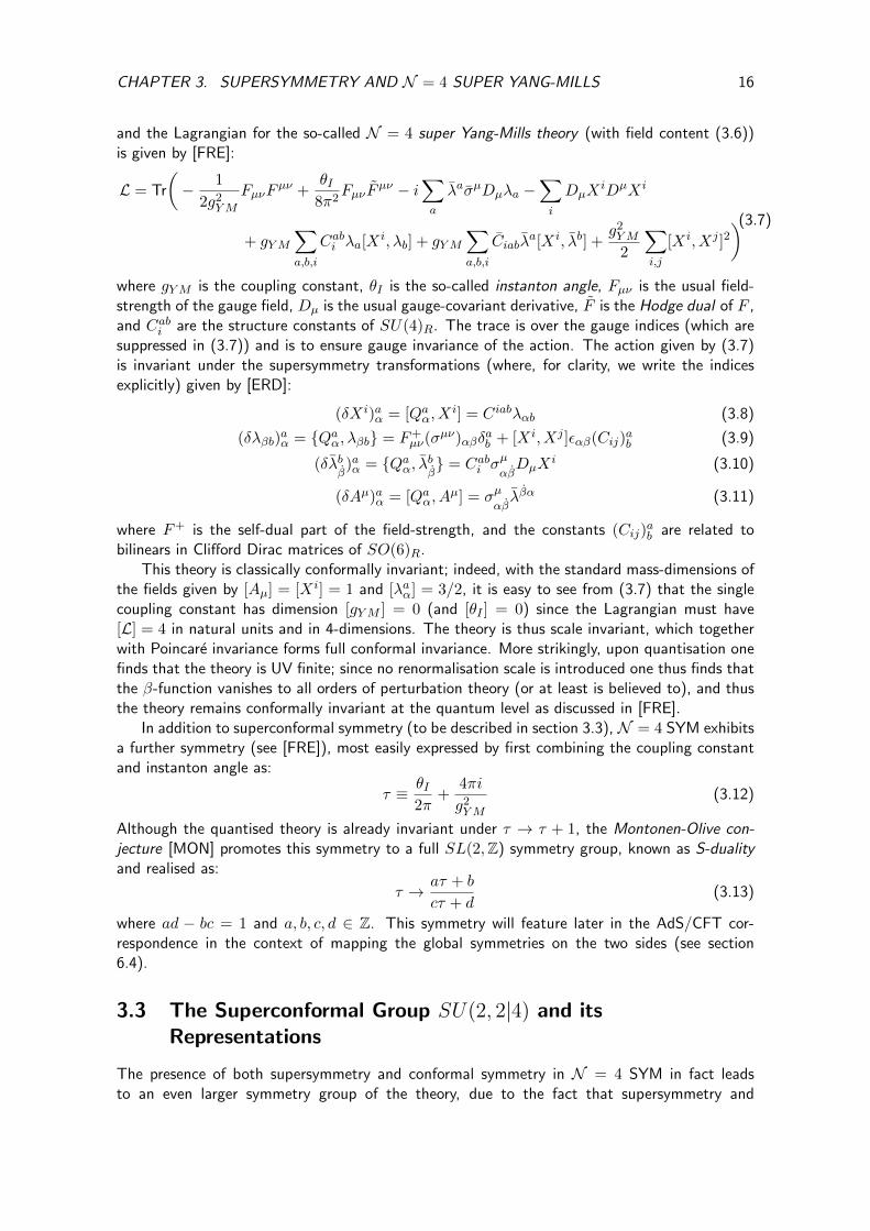
and the Lagrangian for the so-called N = 4 super Yang-Mills theory (with field content (3.6))is given by [FRE]:
L = Tr
(− 1
2g2YM
FµνFµν +
θI8π2
FµνFµν − i
∑a
λaσµDµλa −∑i
DµXiDµXi
+ gYM∑a,b,i
Cabi λa[Xi, λb] + gYM
∑a,b,i
Ciabλa[Xi, λb] +
g2YM
2
∑i,j
[Xi, Xj ]2)(3.7)
where gYM is the coupling constant, θI is the so-called instanton angle, Fµν is the usual field-strength of the gauge field, Dµ is the usual gauge-covariant derivative, F is the Hodge dual of F ,and Cabi are the structure constants of SU(4)R. The trace is over the gauge indices (which aresuppressed in (3.7)) and is to ensure gauge invariance of the action. The action given by (3.7)is invariant under the supersymmetry transformations (where, for clarity, we write the indicesexplicitly) given by [ERD]:
(δXi)aα = [Qaα, Xi] = Ciabλαb (3.8)
(δλβb)aα = Qaα, λβb = F+
µν(σµν)αβδab + [Xi, Xj ]εαβ(Cij)
ab (3.9)
(δλbβ)aα = Qaα, λbβ = Cabi σ
µ
αβDµX
i (3.10)
(δAµ)aα = [Qaα, Aµ] = σµ
αβλβα (3.11)
where F+ is the self-dual part of the field-strength, and the constants (Cij)ab are related to
bilinears in Clifford Dirac matrices of SO(6)R.This theory is classically conformally invariant; indeed, with the standard mass-dimensions of
the fields given by [Aµ] = [Xi] = 1 and [λaα] = 3/2, it is easy to see from (3.7) that the singlecoupling constant has dimension [gYM ] = 0 (and [θI ] = 0) since the Lagrangian must have[L] = 4 in natural units and in 4-dimensions. The theory is thus scale invariant, which togetherwith Poincare invariance forms full conformal invariance. More strikingly, upon quantisation onefinds that the theory is UV finite; since no renormalisation scale is introduced one thus finds thatthe β-function vanishes to all orders of perturbation theory (or at least is believed to), and thusthe theory remains conformally invariant at the quantum level as discussed in [FRE].
In addition to superconformal symmetry (to be described in section 3.3), N = 4 SYM exhibitsa further symmetry (see [FRE]), most easily expressed by first combining the coupling constantand instanton angle as:
τ ≡ θI2π
+4πi
g2YM
(3.12)
Although the quantised theory is already invariant under τ → τ + 1, the Montonen-Olive con-jecture [MON] promotes this symmetry to a full SL(2,Z) symmetry group, known as S-dualityand realised as:
τ → aτ + b
cτ + d(3.13)
where ad − bc = 1 and a, b, c, d ∈ Z. This symmetry will feature later in the AdS/CFT cor-respondence in the context of mapping the global symmetries on the two sides (see section6.4).
3.3 The Superconformal Group SU(2, 2|4) and itsRepresentations
The presence of both supersymmetry and conformal symmetry in N = 4 SYM in fact leadsto an even larger symmetry group of the theory, due to the fact that supersymmetry and

CHAPTER 3. SUPERSYMMETRY AND N = 4 SUPER YANG-MILLS 17
special conformal transformations do not commute, and thus their commutator gives a newsymmetry generator. The full group is known as the superconformal group and is given bythe supergroup SU(2, 2|4), where the notation labels the components of the bosonic subgroupSU(2, 2)× SU(4)R. We briefly sketch the different components leading to this full global con-tinuous symmetry group of N = 4 SYM as in [FRE]:
• Conformal Symmetry: This forms the subgroup SO(2, 4) ∼= SU(2, 2) and is generatedby Pµ,Mµν , D and Kµ, with algebra given as in section 2.2.
• R-symmetry: This forms the subgroup SO(6)R ∼= SU(4)R and is generated by TA withA = 1, 2..., 15. Note that this commutes with the conformal symmetry subgroup.
• Poincare Supersymmetry: This is generated by the spinor supercharges Qaα and theirconjugates, with algebra given as in section 3.1. This does not commute with the entireconformal symmetry subgroup.
• Conformal Supersymmetry: This is generated by Sαa and their conjugates Sαa, whicharise because of the non-commutativity between supersymmetry and special conformaltransformations. They satisfy the following structure relations:
Sαa, Sβb = Qaα, Sbβ = 0 (3.14)
Sαa, Sbβ = 2σµαβKµδ
ba (3.15)
Qaα, Sβb = εαβ(δabD + T ab ) + 12δabMµν(σµν)αβ (3.16)
Representations of the superconformal algebra are built in a similar way to representationsof the conformal and supersymmetry algebras (c.f. sections 2.3 and 3.1). We wish to constructgauge invariant operators which are polynomials in the elementary fields; the gauge invariance isnecessary for the operators to be physical observables, and the polynomial condition means thatthe operators have a definite dimension as is required to form a representation of the conformalgroup. One defines a superconformal primary operator O by:
[S,O = 0 (3.17)
which means that O is the lowest dimensional operator in the representation, the existenceof which is again required by unitarity; the conformal supercharges S have dimension [S] =−1/2 and so successive operation of these supercharges lowers the dimension. The notation[, denotes a commutator or anti-commutator for bosonic or fermionic O respectively. Notethat this definition encompasses (from the superconformal algebra relation (3.15)), but is notequivalent to, the definition of a conformal primary operator, given previously in section 2.3 as[Kµ,O] = 0. One can then define the other operators O′ in the superconformal multiplet as thesuperconformal descendants of the superconformal primary operator:
O′ = [Q,O (3.18)
where the scaling dimensions are clearly related by ∆O′ = ∆O+1/2 since [Q] = 1/2. In analogyto the conformal multiplet case, a superconformal descendant is never a superconformal primaryoperator, since there is always an operator of lower dimension. A superconformal multiplet thenconsists of a single superconformal primary operator and its descendants.
With this condition in mind, one can show as described in [FRE] that the gauge invariantsuperconformal primary operators in N = 4 SYM are given by the scalars only, albeit in a

CHAPTER 3. SUPERSYMMETRY AND N = 4 SUPER YANG-MILLS 18
symmetrised manner; one shows this essentially by using the SUSY transformations (3.8)-(3.11)and the fact that a superconformal primary can never be a Q-(anti)commutator of anotheroperator, since it would then be a superconformal descendant. The simplest such operators arethe so-called single trace operators (where the trace is to ensure the operator is gauge invariant)defined as [FRE]:
On ≡ Tr[X(i1Xi2 ...Xin)] (3.19)
where we see that the SO(6)R indices are symmetrized in the trace. This is in fact generally areducible representation of the R-symmetry, and one may further decompose it into a trace anda traceless symmetric part. As mentioned previously, all fields in the N = 4 gauge multiplettransform in the adjoint representation of the gauge group, and are thus traceless hermitianmatrices. One thus has Tr[Xi] = 0 and so the simplest irreducible operators one can form aregiven by [FRE]:
Konishi Multiplet: Tr[XiXi]
Supergravity Multiplet: Tr[XiXj](3.20)
where summation over i is implied in the first expression, and ij denotes the traceless part inthe second (with symmetrisation true automatically by virtue of the cyclic property of the trace).The latter name is pre-emptive of the field/operator map in the AdS/CFT correspondence thatwe will discuss in section 7.1.
The supergravity multiplet is the simplest example of a superconformal 1/2-BPS multiplet, so-called because they are annihilated by half of the supercharges and thus are shortened multiplets,in analogy with the supersymmetric BPS multiplets mentioned in section 3.1. BPS multipletsplay a very important role in testing the AdS/CFT correspondence and so it is worth unpackingthis analogy a bit. Representations of the superconformal algebra are labelled by their Lorentzquantum numbers and scaling dimension, as for the conformal case, but are also labelled by theDynkin labels [r1, r2, r3] of the R-symmetry group SU(4)R discussed previously; they are thuslabelled fully by the quantum numbers of the bosonic subgroup. In the same way that unitarityled to the BPS bound in section 3.1, unitarity here requires that the conformal dimension isbounded from below by the spin and R-symmetry quantum numbers (see [FRE]); considering onlythe primaries (since these have the lowest dimension anyway), we mentioned before that theseare scalars and hence have vanishing Lorentz quantum numbers, meaning that the conformaldimension is bounded below by the R-symmetry charges only. When this bound is saturatedone again has shortened multiplets (i.e. the primary, known in this case as a chiral primary, isannihilated by some of the supercharges), with the conformal dimension related directly to theR-symmetry charges. These are known in this context as BPS multiplets and are very importantsince the conformal dimension is protected by the representation theory and thus does not receivequantum corrections; this is useful for testing the AdS/CFT correspondence since, as we shallsee, when one considers the classical supergravity regime on the string side (which is the easiestfor calculations) one simultaneously has the strong-coupling regime on the gauge theory side, forwhich it is not possible to calculate quantum corrections using perturbation theory. Protectedor unrenormalised quantities are thus particularly important for testing the correspondence. Weillustrate these concepts by briefly summarising some properties of superconformal multipletsbelow as in [FRE]:
Operator SU(4)R primary Dimension
1/2 BPS [0, k, 0], k ≥ 2 k
1/4 BPS [l, k, l], l ≥ 1 k + 2l
1/8 BPS [l, k, l + 2m] k + 2l + 3m, m ≥ 1
Non-BPS Any Unprotected

Chapter 4
Superstrings and Supergravity
The AdS/CFT correspondence states the equivalence between the N = 4 SYM theory describedin chapter 3, and Type IIB superstring or supergravity theory (depending on the regime) definedon AdS5×S5. In this section we provide a brief review of string theory up to the point of beingable to discuss the essential features of Type IIB superstring theory (such as its field contentand symmetries), as well as its supergravity limit. Properties of D-branes will also be discussed,which play a crucial role in the AdS/CFT correspondence.
4.1 Review of the Bosonic String
The bosonic string, although fundamentally incomplete, is important as many of its featuresstill play a role in superstring theory. It is thus worth devoting some time to understand itsanalysis. The string action for bosonic string theory in d-dimensional flat spacetime is given bythe Polaykov action [POL]:
SP = − 1
4πα′
∫d2σ√−hhαβ∂αXµ∂βX
νηµν (4.1)
Some clarifications of (4.1) are in order: the fields Xµ(τ, σ) are the embedding of the 2-dimensional string worldsheet (with coordinates σα = (τ, σ)) in spacetime, hαβ is the worldsheetmetric, and α′ is a constant known as the slope parameter, related to the string tension byT = 1/(2πα′). This is known as the first-order action, and varying with respect to hαβ andusing the resulting equations of motion gives the second-order Nambu-Goto action [POL]:
SNG = − 1
2πα′
∫d2σ√−det[∂αXµ∂βXνηµν ] (4.2)
which is simply the proper area of the worldsheet (in analogy to the action for the relativisticpoint particle which is given by the proper length of the worldline).
The Polyakov action is more desirable than the Nambu-Goto action for several reasons;the lack of the square-root allows for quantisation more easily, but furthermore (4.1) exhibitsa symmetry not present in (4.2). Although both actions exhibit manifest spacetime Poincareinvariance and worldsheet diffeomorphism invariance σα → σα(σβ), (4.1) also has worldsheetWeyl or conformal invariance (see [POL]):
hαβ(τ, σ)→ eω(τ,σ)hαβ(τ, σ) (4.3)
for any ω(τ, σ). Worldsheet diffeomorphism together with Weyl invariance allows us to fix the 3independent components of the 2D worldsheet metric, and using the so-called conformal gauge,where hαβ = ηαβ, the action (4.1) reduces to:
SC = − 1
4πα′
∫d2σ(X2 −X ′2) (4.4)
19

CHAPTER 4. SUPERSTRINGS AND SUPERGRAVITY 20
where X2 ≡ ∂τXµ∂τXµ and X ′2 ≡ ∂σX
µ∂σXµ. The equations of motion for Xµ derivedfrom (4.4) are simply the 2D wave equations, but one must not forget that there are additionalconstraints associated with the fact that there is a gauge symmetry (which was exploited inderiving (4.4)). These Virasoro constraints [CAC] are simply given by the equations of motionfor the worldsheet metric, which can also be expressed as:
δSPδhαβ
∝ Tαβ = 0 (4.5)
i.e. the worldsheet energy-momentum tensor must vanish. Altogether, one must then solve theset of equations:
(∂2τ − ∂2
σ)Xµ = 0
(X ′ ± X)2 = 0(4.6)
In addition to the equations of motion (and the constraints), in the variation of (4.4) oneencounters a boundary term:
δSC |boundary ∝∫ ∞−∞
dτ(X ′ · δX|σ=π −X ′ · δX|σ=0
)(4.7)
which must also vanish. There are multiple ways of ensuring (4.7) vanishes:
• Open String: If the endpoints of the string (σ = 0, π) are distinguished, then (4.7) maybe made to vanish by taking:
X ′µ(τ, σ∗) = 0 or Xµ(τ, σ∗) = xµσ∗ (4.8)
for some fixed xµσ∗ , and where σ∗ represents a string endpoint (σ = 0 or π). These areknown as Neumann and Dirichlet boundary conditions respectively. Dirichlet boundaryconditions (for which the endpoint is fixed) lead naturally to the concept of D-branes,which are objects upon which open strings end; these will be discussed in greater detail insection 4.4.
• Closed String: If the endpoints of the string are to be identified, then (4.7) will vanishwith the periodic boundary conditions:
Xµ(τ, π) = Xµ(τ, 0) (4.9)
One then proceeds in a similar way to standard QFT i.e. construct solutions to (4.6) viamode expansions, ensuring that they are consistent with the boundary conditions chosen. As anexample, the mode expansion [CAC]:
Xµ(τ, σ) = xµ +√
2α′αµ0τ + i√
2α′∑m6=0
αµmme−imτcos(mσ) (4.10)
is a solution for the open string with Neumann boundary conditions at both endpoints, wherexµ is some fixed number. One then quantises the theory in the usual way, by imposing theequal-time commutation relations:
[Xµ(τ, σ), Xν(τ, σ′)] = 0 (4.11)
[Xµ(τ, σ), P ν(τ, σ′)] = ηµνδ(σ − σ′) (4.12)

CHAPTER 4. SUPERSTRINGS AND SUPERGRAVITY 21
where Pµ ≡ ∂L/∂Xµ is the canonical momentum conjugate to the field Xµ. Using these togetherwith the mode expansion for Xµ, one can then find the implied commutation relations for theexpansion coefficients αµm, which are now operators in the quantum theory. One finds (see [ZWE])an infinite set of harmonic oscillators for the rescaled expansion coefficients aµm ≡ αµm/
√m and
their conjugates, which may thus be interpreted as creation and annihilation operators.The spectrum can then be constructed in the usual way; define a vacuum state |0〉 by the
condition aµm |0〉 = 0 for all values of m, and then construct the rest of the spectrum as the statesaµmaνn... |0〉. The exact procedure is known as light-cone gauge quantisation and makes use of theworldsheet symmetries to remove negative norm states which threaten unitarity (see [ZWE] for
details). The spectrum is built level-by-level in the number operator N ≡∑∞
m=1
∑D−2i=1 ma†imaim,
where the upper bound (D − 2) on the i-summation is a result of removing redundant gaugedegrees of freedom in the light-cone gauge quantization procedure. One finds the followingparticle content (where M represents the mass of the state) in the lower levels of the open andclosed string spectra (see [ZWE]):
Open String Closed String
N = 0 (M2 < 0) T T
N = 1 (M = 0) Aµ gµν , Bµν , Φ
where the tachyon T has negative mass, Aµ is a vector, gµν is a 2nd-rank symmetric tracelesstensor (graviton), Bµν is a 2-form, and Φ is a scalar (dilaton). The higher level states areall massive, and will generally be ignored throughout; we mention in passing however that themasses depend inversely on α′ and thus become very large in the limit α′ → 0. Note also that,although in principle problematic, the tachyons are in fact projected out in the full superstringtheory (to be discussed later), via the so-called GSO projection (see [POL]).
It is worth noting that, as is clear from the stated form of the number operator N , manifestLorentz invariance is lost in the light-cone gauge quantization procedure (this is not so in themore complicated covariant quantisation procedure [ZWE], but we will not discuss this further).The requirement that Lorentz invariance be preserved actually leads to a remarkable prediction.One can construct worldsheet currents associated with Lorentz transformations in the usual way,and the associated conserved charges are given in the string theory by [CAC]:
Jµν =1
2πα′
∫ π
0dσ(XµXν − XνXµ)
= xµP ν − xνPµ + i∑m 6=0
1
m(αµ−mα
νm − αν−mαµm)
(4.13)
Using the commutation relations for the oscillators αµm, one can then check whether the Jµν obeythe usual Lorentz algebra. It turns out that they do indeed satisfy the Lorentz algebra providedthat D = 26, known as the critical dimension; in this manner, the requirement that the theory beLorentz invariant essentially predicts the dimensionality of spacetime. Since we seem to observeD = 4, we are led to the idea of Kaluza-Klein reduction [FRE], which involves compactifyingcertain spatial dimensions on compact spaces such as circles or tori, and then letting the size ofthese compactified dimensions go to zero. In this way, one can derive a lower dimensional theoryfrom a higher dimensional one. We shall mention this procedure again in chapter 7.

CHAPTER 4. SUPERSTRINGS AND SUPERGRAVITY 22
4.2 Coupling the Bosonic String to a Background and EffectiveSpacetime Actions
The natural generalisation of the previous section is to consider the string propagating in abackground of its own massless modes (for the graviton this corresponds to the string propagatingin a curved spacetime, for example). For the closed string this can be achieved via the action(see [CAC]):
S = − 1
4πα′
∫d2σ√−hhαβ∂αXµ∂βX
νgµν(X)
− 1
4πα′
∫d2σ
(εαβ∂αX
µ∂βXνBµν(X)−
√−hα′R(2)Φ(X)
) (4.14)
where R(2) is the Ricci scalar on the 2D worldsheet, and εαβ is the 2D antisymmetric symbol.This is known as the non-linear sigma model ; note that the first term is just the Polyakov action(4.1) but with a general target space metric gµν(X), and the other two terms are appropriategeneralisations to the other massless fields of the closed string spectrum. The quantity:
1
4π
∫d2σ√−hR(2) = χ ≡ 2− 2g (4.15)
is a topological invariant known as the Euler characteristic [FRA], where g is the genus of theworldsheet i.e. the number of holes. In string perturbation theory, one calculates amplitudes byconsidering a path integral of the form (see [VIE]):
String amplitude =∑g
(gs)2g−2
∫Σg
DXe−S[X]V1...Vn (4.16)
where g is the genus as above, Σg represents all surfaces of genus g, gs is the string couplingconstant, and Vi are so-called vertex operators. The string coupling constant can be understoodas follows. If the dilaton acquires a non-zero vacuum expectation value, Φ → φ + Φ, then wesee from above that the path integral includes a multiplicative factor of e−χφ = eφ(2g−2). From(4.16) we thus see that it is natural to identify the (closed) string coupling constant as gs = eφ;increasing the genus by 1, and thus adding a hole to the worldsheet, then contributes a factorof e2φ = g2
s . For the open string one has instead gs = eφ/2. These facts will be important whenwe state the AdS/CFT correspondence in chapter 6.
In making the transition from the action (4.1) to (4.14), it is important that we maintainworldsheet Weyl or conformal invariance. As mentioned in section 2.3, this can be expressed asthe vanishing of the renormalisation-group beta functions; there will be three independent betafunctions here, as gµν , Bµν and Φ can each be interpreted as a coupling in the string action(4.14). To leading order in α′ (which corresponds to the low energy limit i.e. α′ → 0), one findsthe beta functions (see [CAC]):
β(g)µν = α′
(Rµν + 2∇µ∇νΦ− 1
4HµλρH
λρν
)β(B)µν = α′
(−1
2∇λHλµν +∇λΦHλµν
)(4.17)
β(Φ) = α′(−1
2∇2Φ +∇µΦ∇µΦ− 1
24HµνλH
µνλ
)where H3 ≡ dB3 is the 3-form field-strength associated with the 2-form B2, and Rµν is thespacetime Ricci tensor associated with the graviton gµν . Clearly, the vanishing of the beta-functions in (4.17) looks like a set of field equations for the massless spacetime fields of the

CHAPTER 4. SUPERSTRINGS AND SUPERGRAVITY 23
string spectrum. The natural question arises as to whether these fields equations may be derivedfrom an action principle; this is a non-trivial statement since the existence of an associated actionin general depends on certain integrability conditions. Remarkably, the field equations can bederived from the following spacetime action [CAC]:
Seff. =
∫d26x
√−detge−2Φ
(R− 1
12HµνλH
µνλ + 4∇µΦ∇µΦ
)(4.18)
which is known as the effective spacetime action of the (closed) bosonic string theory. Thisprocedure of deriving an effective spacetime field theory by demanding conformal invariance ofthe worldsheet theory is crucial, and in the superstring case leads to the derivation of supergravitytheory as the low energy approximation of string theory.
4.3 Superstrings and Type IIB Theory
The bosonic string, although illustrative, is incomplete for several reasons. Perhaps most im-portantly, the spectrum does not contain any fermions, and so there is no hope of somehowrecovering the standard model of particle physics. Furthermore, both the open and closed stringspectra contain a problematic tachyon state, and the critical dimension D = 26 is somewhat farfrom the 4-dimensions we appear to live in.
Following the RNS formalism, we thus consider a supersymmetric completion of the Polyakovaction by introducing worldsheet fermions (which, note, are still spacetime vectors) Ψµ via theaction (expressed in conformal gauge) [CAC]:
S = − 1
4πα′
∫d2σ
(∂αXµ∂
αXµ + iΨµρα∂αΨµ
)(4.19)
where ρα, ρβ = 2ηαβ and Ψ ≡ iΨ†ρ0 (we use the notation ρα to emphasise that these are notthe familiar 4-dimensional γ-matrices). Decomposing the worldsheet fermion into Weyl spinorsΨµ = (ψµ−, ψ
µ+), choosing a particularly simple representation for ρα, and using worldsheet light-
cone coordinates σ± ≡ τ ± σ, the fermionic part of the action can then be written as [CAC]:
SΨ = − 1
2πα′
∫d2σ
(ψµ−∂+ψµ− + ψµ+∂−ψµ+
)(4.20)
One can then vary this action to obtain the equations of motion:
∂−ψµ+ = ∂+ψ
µ− = 0 (4.21)
and so there are separate right and left-moving waves, as in the bosonic case (c.f. solutions tothe wave equation in (4.6)). There are again additional constraints associated with the gaugeinvariance, which are still expressed as Tαβ = 0, though the introduction of the fermionic actionnow changes the form of the worldsheet energy-momentum tensor.
Furthermore, in varying the action (4.20), one encounters a new boundary term:
δSΨ|boundary ∝∫dτ(ψµ−δψ−µ − ψ
µ+δψ+µ
)|σ=πσ=0 (4.22)
which must be made to vanish (note that the first-order nature of the fermionic action has led tothere being no derivatives in this boundary term, in contrast to the bosonic sector). For the openstring (which has distinct endpoints and thus the σ = 0, π contributions must independentlyvanish) this can be achieved in two ways:

CHAPTER 4. SUPERSTRINGS AND SUPERGRAVITY 24
• Ramond Sector (R): ψµ+(τ, π) = +ψµ−(τ, π).
• Neveu-Schwarz Sector (NS): ψµ+(τ, π) = −ψµ−(τ, π).
where, note, there is also a freedom in choosing ψµ+(τ, 0) = ±ψµ−(τ, 0), but these are redundant(i.e. not physically different) and so one imposes ψµ+(τ, 0) = +ψµ−(τ, 0) by convention (see[CAC]). For the closed superstring, the vanishing of (4.22) must occur in a different manneri.e. by cancelling the contribution ψµ±δψ±µ|σ=π with ψµ±δψ±µ|σ=0, where the ± are correlatedthroughout. There are 4 different ways of achieving this:
ψµ+(τ, σ) = ±ψµ+(τ, σ + π)
ψµ−(τ, σ) = ±ψµ−(τ, σ + π)(4.23)
leading to 4 sectors of the closed superstring theory: R-R, R-NS, NS-R, and NS-NS, where Rrefers to periodic and NS to anti-periodic boundary conditions.
One then proceeds as in the bosonic string case, by considering mode expansion solutionsof the equations of motion consistent with the relevant boundary conditions, and quantizingby promoting the fields to operators; the expansion coefficients of the worldsheet fermions nowbecome operators satisfying certain anti-commutation relations. One uses again the light-conegauge quantization procedure, now appealing to the superconformal symmetry of the theory toremove negative-norm states and preserve unitarity. There is a different vacuum state for the Rand NS sectors; the NS vacuum state is a tachyon whereas the R vacuum state is a spacetimespinor (we thus see that spacetime fermions have indeed arisen from the inclusion of a worldsheetfermionic action). The GSO projection mentioned previously projects out the tachyon, as wellas one of the chiralities of the R vacuum. For the closed string (which, recall from above, islike a tensor product of open strings), it turns out there are then only 2 inequivalent choices ofvacuum, which give rise to different closed superstring theories known as Type IIA/B, both withcritical dimension D = 10 (see [POL] for details). Our focus for the AdS/CFT correspondencewill be on Type IIB, which has the following massless spectrum [CAC]:
RR A0, A2, A+4
R-NS Ψ1+, χ
1−
NS-R Ψ2+, χ
2−
NS-NS Φ, B2, gµν
where An is an n-form (and A+4 is self-dual), ΨI
+ (I = 1, 2) are right-handed dilatini, χI−(I = 1, 2) are left-handed gravitini, and the NS-NS sector is just the massless sector of theclosed bosonic string spectrum that we have seen previously. We see that the theory is chiralsince the 2 dilatini and the 2 gravitini have the same chirality.
As in the bosonic string case, Type IIB string theory has a low energy effective spacetimetheory, which remarkably turns out to be a supergravity theory (i.e. a supersymmetric theory ofgravity, here with N = 2). It is not possible to write a complete action for the theory due to thepresence of the self-dual 4-form A+
4 , but one can write an action that includes both dualities, andthen supplement this with the self-duality condition ∗F5 = F5 where F5 is the 5-form F5 ≡ dA4
and ∗ is the Hodge dual. The bosonic part of this action then has the form [FRE]:
SIIB =1
4κ2
∫d10x
√−detge−2Φ
(2R+ 8∇µΦ∇µΦ− |H3|2
)− 1
4κ2
∫d10x
[√−detg
(|F1|2 + |F3|2 +
1
2|F5|2
)+A+
4 ∧H3 ∧ F3
]+ Sfermions
(4.24)

CHAPTER 4. SUPERSTRINGS AND SUPERGRAVITY 25
where κ is the coupling constant, Fn ≡ dAn−1 is the n-form field-strength, H3 is the 3-formH3 ≡ dB2, F3 ≡ F3−A0H3 and F5 ≡ F5− 1
2A2∧H3 + 12B2∧F3. The Type IIB action exhibits
a non-compact SU(1, 1) ∼= SL(2,R) symmetry (see [FRE]), most manifest in the Einstein framewhich is obtained from the string frame above as:
gµν → e−Φ/2gµν (4.25)
The Einstein frame is so-called because, as is clear, the Type IIB action then contains the usualEinstein-Hilbert action familiar from general relativity. Combining the axion A0 and the dilatoninto a complex scalar τ ≡ A0 + ie−Φ, the symmetry transformation is then given by:
τ → aτ + b
cτ + d(4.26)
where a, b, c, d ∈ R and ad − bc = 1. Note that in the quantum theory there is a quantizationcondition τ ∼= τ + 1, and thus the symmetry group reduces to the subgroup SL(2,Z). Thissymmetry will feature later in the AdS/CFT correspondence (see section 6.4).
4.4 Branes in Supergravity and Superstring Theory
We have seen previously that objects known as D-branes arise in string theory as hyperplanesupon which open string endpoints with Dirichlet boundary conditions are fixed. D-branes can infact be seen to arise from a different point of view; indeed, this dual interpretation is of greatsignificance in motivating the AdS/CFT correspondence as we shall see in section 6.2. We nowdiscuss this alternative point of view by considering particular solutions to supergravity theoryfollowing [FRE], and then mention how the two points of view converge. We will then brieflydiscuss the important subject of gauge theories living on the worldvolumes of branes.
It is natural to consider a (p + 1)-form Ap+1 as coupling to an object Σp+1 of dimensionp+ 1 because one can construct the action:
Sp+1 ∝∫
Σp+1
Ap+1 (4.27)
which is diffeomorphism invariant since the form is being integrated over a manifold of dimen-sion equal to the form’s rank (see [NAK]). The action (4.27) is also invariant under the gaugetransformation Ap+1 → Ap+1 +dρp, and we note that the field-strength Fp+2 ≡ dAp+1 is clearlygauge invariant since the exterior derivative is nilpotent (the field-strength also has a conservedflux). We can then define a p-brane to be a solution of the supergravity field equations that hasa non-zero charge associated to the gauge field Ap+1. The possible brane solutions in a givensupergravity theory are thus limited by what p-forms are present in the field content. Type IIBsupergravity, for example, contains the following brane solutions:
Brane Couples to: Dual BraneD(-1) τ D7
F1 B2 NS5
D1 A2 D5
D3 A+4 D3
Some clarifications of nomenclature are in order:
• A p-brane associated with a gauge field Ap+1 that is in the R-R sector is known as aDp-brane. The similarity of name with the aforementioned D-branes is not an accident,and will be explained later in this section.

CHAPTER 4. SUPERSTRINGS AND SUPERGRAVITY 26
• The 1-brane that couples to the NS-NS field B2 is known as the fundamental string F1;this is intuitive, given the coupling of the original string to this 2-form in the action (4.14).The prefix ‘NS’ in NS5 simply labels the fact that the 2-form B2 is an NS-NS field.
• The D(-1) brane is localised not only in all spatial directions but also in time, and is thusan instanton.
• The dual of a p-brane (coupled to a (p+ 1)-form) is the (D− 4− p)-brane coupled to the(D − 3− p)-form that is the Poincare dual of the (p+ 1)-form, defined by:
dAdualD−3−p ≡ ∗dAp+1 (4.28)
We will focus here on Dp-branes, and in particular D3-branes (which, note, are self-dual), sincethese are of most relevance for the AdS/CFT correspondence.
In D = 10, a p-brane solution to supergravity theory has symmetry group Rp+1×SO(1, p)×SO(9− p) i.e. the solution contains a flat hypersurface of dimension (p+ 1) which has Poincareinvariance Rp+1×SO(1, p), and the (9−p)-dimensional transverse space has maximal rotationalinvariance SO(9−p). Each brane solution breaks half of the supersymmetries of the supergravitytheory [FRE] i.e. it is an example of a 1/2 BPS solution (c.f. section 3.1). Denoting thecoordinates parallel to the brane as xµ and those perpendicular to the brane as yi, an ansatzthat has the above symmetry and satisfies the supergravity field equations is given by:
ds2 =1√H(~y)
ηµνdxµdxν +
√H(~y)d~y2 (4.29)
where, furthermore, eΦ = [H(~y)](3−p)/4 and H(~y) must be a harmonic function of ~y. Requiringthat flat space be recovered far away from the brane (i.e. in the limit y ≡
√~y · ~y → ∞) fixes
the function H(~y) to take the form:
H(~y) = 1 +
(L
y
)D−p−3
(4.30)
where L is some scale factor; we write D for generality, but recall that the case of interest isD = 10. Of particular importance to the AdS/CFT correspondence will be the solution for astack of N coincident Dp-branes, for which one finds:
LD−p−3 = Ngs(4π)(5−p)/2Γ
(7− p
2
)α′(D−p−3)/2 (4.31)
where the factor of N comes from N units of 5-form flux sourced by the N branes. We will usethe solution (4.29)-(4.31) in chapter 6 when we discuss the decoupling argument.
In addition to the supergravity limit of superstring theory (α′ → 0) discussed previously,another well-defined limit of string theory is the weak coupling limit gs → 0, which is the stringperturbation theory regime (c.f. equation (4.16)). It turns out that Dp-branes also have ags → 0 limit, whereas other p-branes do not. Indeed, we see from (4.29)-(4.31) that in thislimit H(~y) → 1 and thus the metric becomes flat everywhere except at y = 0; on this (p + 1)-dimensional hypersurface the metric is in fact singular. Thus we see that, in the weak couplinglimit, Dp-brane solutions to supergravity become localised defects in spacetime; as discussedin [FRE], it turns out that the interaction with a string propagating in such a background isdescribed entirely by the boundary conditions of the string on the brane, which turn out to beNeumann conditions parallel to the brane and Dirichlet conditions perpendicular to it. In this

CHAPTER 4. SUPERSTRINGS AND SUPERGRAVITY 27
manner, we see that the Dp-branes introduced as solutions of supergravity are precisely theD-branes introduced earlier in open string theory.
To conclude this chapter we discuss the important subject of how gauge theories arise onthe worldvolumes of D-branes; this is of utmost relevance to the AdS/CFT correspondence, andso we shall review the topic but not discuss the exact details of open string quantization in thepresence of D-branes (see [ZWE] for details). Let us first consider an open string with bothendpoints fixed on a single D-brane. Clearly, the length of the string may become arbitrarilyshort in which case there is no tension; the string mode must then be massless, and it is possibleto show that it is in fact a vector Aµ in the worldvolume i.e. there is a U(1) gauge theory onthe worldvolume of the brane. If we consider instead a stack of N coincident branes then wemust further label the string states by indices which denote which brane the endpoints lie on.These are known as Chan-Patton factors [ZWE], and for N branes there will be N2−N possiblestring configurations leading to N2−N massless modes [Aµ]ij on the worldvolume of the branes,where i, j = 1...N . One then finds a U(N) gauge theory on the brane worldvolume; in fact, thefactor of U(1) = U(N)/SU(N) corresponds to the overall position of the branes in spacetime,and thus is not relevant for considering the dynamics on the brane worldvolume itself, which isthen described by an SU(N) gauge theory (separating the branes would give the modes massand thus correspond to spontaneously breaking the gauge symmetry, but we shall not need suchmechanisms in the following). As mentioned previously, each brane solution breaks half of thePoincare superymmetries and so, in particular, for a stack of N D3-branes, the brane dynamicsis described by 4-dimensional N = 4 SYM theory with gauge group SU(N) (see [FRE]). Thisfact will be very important in chapter 6 when we discuss the decoupling argument.

Chapter 5
Anti-de Sitter Space
The Type IIB theory on the gravity side of the correspondence is taken to be in an AdS5 × S5
background. In this chapter we define the anti-de Sitter space AdSd and discuss its essentialfeatures including isometries, important coordinate systems and the conformal boundary.
5.1 Definition of Anti-de Sitter Space
Let us first define the concept of a maximally symmetric space of d-dimensions [ZEE], meaningthat it has the maximum number of Killing vectors possible for a d-dimensional manifold, namelyd(d + 1)/2 (corresponding locally to d translations and d(d − 1)/2 rotations). A maximallysymmetric space can be understood intuitively as one that is homogeneous and isotropic at some(and thus every) point, meaning it looks the same in all directions and at all positions. Maximalsymmetry provides d(d − 1)/2 constraints on the Riemann curvature tensor, which turn out tobe enough to fix its form uniquely as (see [ZEE]):
Rµνρσ = C(gµρgνσ − gµσgνρ) (5.1)
for some constant C, and thus one finds by contracting that Rµν = (d − 1)Cgµν and R =d(d− 1)C i.e. maximally symmetric spaces have constant curvature scalars.
The anti-de Sitter space (AdS) is a space of Lorentzian signature and (as we shall see)constant negative curvature. In a similar fashion to other constant curvature spaces (e.g. thesphere), AdS space may be defined as an embedding in a higher-dimensional space. If we considera flat embedding space R2,d−1 with coordinates Xa (a = 0...d) and metric:
ds2 = −dX20 − dX2
d +d−1∑i=1
dX2i (5.2)
then we may define AdSd as the set of solutions of:
X20 +X2
d −d−1∑i=1
X2i = L2 (5.3)
where L is known as the AdS radius. We also mention briefly that Euclidean AdSd may bedefined in an analogous way, but embedded instead in R1,d and with the defining equation:
X20 −X2
d −d−1∑i=1
X2i = L2 (5.4)
Indeed, the Euclidean version of AdS will in fact be used later in chapter 7 when we discuss testsof the correspondence, and the results discussed below translate simply.
It is obvious from the defining equations that the isometry group of AdSd is O(2, d− 1) (orO(1, d) for the Euclidean case); restricting to our case of interest, AdS5, we thus see that the
28

CHAPTER 5. ANTI-DE SITTER SPACE 29
isometry group is O(2, 4), a group we encountered previously in section 2.2 as the (extended)conformal group in 4-dimensional Minkowski space. The space AdSd can also be expressed asthe coset manifold SO(2, d − 1)/SO(2, d − 2) i.e. the isometry group minus (by quotient) thesubgroup that leaves a point in the space invariant (in the same way that S2 ∼= SO(3)/SO(2)).Since the dimension of O(2, d−1) is d(d+1)/2 we see that AdSd is indeed a maximally symmetricspace, and thus should have constant curvature scalars.
By eliminating the final coordinate via (Xd)2 = L2 + ηµνXµXν , where µ = (0, 1...d − 1)
and ηµν is the d-dimensional Minkowski metric, we may provide a set of coordinates for AdSdand write the metric as:
ds2 =
(ηµν −
ηµληνρXλXρ
X ·X + L2
)dXµdXν (5.5)
where in an obvious notation X ·X ≡ ηµνXµXν . One can then calculate the Riemann tensor
from this (bearing in mind that, since this is a maximally symmetric space, only the constant Cin (5.1) needs to be fixed) and one finds [ZEE] that C = −1/L2. From the expressions for Rµνand R underneath (5.1) we thus see that AdSd has constant negative curvature scalar and that:
Rµν −1
2gµνR =
(d− 1)(d− 2)
2L2gµν (5.6)
meaning that (in d > 2) AdSd is a solution to the vacuum Einstein field equations with a negativecosmological constant.
5.2 Coordinate Systems on AdSd
Let us for convenience now set L = 1 in (5.3). We may introduce a set of coordinates on AdSdby writing:
X0 = rcost
Xd = rsint (5.7)
Xi = rxi
where∑d−1
i=1 x2i = 1, and the other coordinates range over r, r > 0 and t ∈ [0, 2π). The
defining equation (5.3) then clearly implies r2 − r2 = 1. Finding the differentials dXµ of thecoordinates (5.7) and substituting into the metric (5.2) (together with the fact that
∑i x
2i =
1→∑
i xidxi = 0) we thus find after simple algebra that:
ds2 = −dr2 − r2dt2 + dr2 + r2dΩ2d−2 (5.8)
Using the constraint r2 − r2 = 1 we find that dr2 = r2
r2dr2 and thus more simple algebra gives
the metric:
ds2 = −(1 + r2)dt2 +dr2
1 + r2+ r2dΩ2
d−2 (5.9)
We have thus eliminated r and now have a set of d coordinates for AdSd. We see from (5.9) thatt acts as a time coordinate, yet from it’s definition in (5.7) this coordinate appears to be periodic.As discussed in [ZEE], to avoid the existence of closed timelike curves and casual inconsistencies,we thus unwrap the time coordinate (technically, we move to the universal cover) and simplydefine the space AdSd by equation (5.9) (which is, after all, a solution to the Einstein field

CHAPTER 5. ANTI-DE SITTER SPACE 30
equations) for t ∈ R. Note interestingly that the metric (5.9) for AdSd has the same form asthe Schwarzchild metric:
ds2 = −f(r)dt2 +dr2
f(r)+ r2dΩ2
d−2 (5.10)
but here f(r) = 1+r2 > 0, and thus we see that the anti-de Sitter space does not have an eventhorizon, unlike the Schwarzchild spacetime for which the horizon is defined by the coordinatesingularity when f(r) = 0.
We now make a further coordinate transformation in (5.9) given by r = sinhρ for ρ > 0.Since dr = coshρdρ and 1 + r2 = cosh2ρ we easily find:
ds2 = −cosh2ρdt2 + dρ2 + sinh2ρdΩ2d−2 (5.11)
These are known as global coordinates [ZEE] (so-called because they cover the entire AdSspace). We can make instead a different coordinate substitution in (5.9) given by r = tanβ forβ ∈ [0, π/2). Since dr = sec2βdβ and 1 + r2 = sec2β we easily find the metric:
ds2 =1
cos2β
(−dt2 + dβ2 + sin2βdΩ2
d−2
)=
1
cos2β
(−dt2 + dΩ2
d−1
)(5.12)
where the second equality follows by the general relation dΩ2p+1 = dβ2+sin2βdΩ2
p with β ∈ [0, π](we return to this matter in section 5.3). These are known as conformal coordinates [ZEE], so-called because we see manifestly from (5.12) that AdSd is conformally equivalent to the cylinderR × Sd−1 with metric ds2 = −dt2 + dΩ2
d−1 (note that flat space R1,d−1 is also conformallyequivalent to this cylinder; we return to this in section 5.4).
5.3 The Conformal Boundary of AdSd
We now introduce the important notion of the conformal boundary of AdSd space, a conceptthat may be visualized in a number of ways. We introduce it as in [ZEE] by building on thematerial in the previous section, and in particular the set of conformal coordinates that definedthe metric (5.12).
The coordinate β in the first half of (5.12) clearly plays the role of a latitude; strangely,however, we saw from its definition that it ranges over the values β ∈ [0, π/2) rather than theusual β ∈ [0, π]. Thus, identifying dΩ2
d−1 = dβ2 + sin2βdΩ2d−2 in equation (5.12), although true
locally, is somewhat misleading since the spatial part of AdSd really only covers the northernhemisphere of Sd−1 and not the full sphere. Thus, we really have a hemisphere (after a conformaltransformation, of course) for the spatial part of AdSd, with boundary at the equator; topolog-ically this is equivalent to the ball Bd−1 (e.g. a hemisphere of S2 is topologically equivalent tothe disk B2, as seen via a direct projection onto the plane). We thus see that the spatial sectionsBd−1 of AdSd are bounded by Sd−2 (since ∂Bd = Sd−1), which we commonly associate withRd−2 with spatial infinity identified as a single point (c.f. the Riemann sphere [FRA]). Takingthe time coordinate into account we thus arrive at the important result that AdSd is boundedby Minkowski space R1,d−2:
∂(AdSd) = R1,d−2 (5.13)
This result is of crucial importance in the AdS/CFT correspondence, and is at the heart of itsholographic nature.

CHAPTER 5. ANTI-DE SITTER SPACE 31
5.4 Poincare Coordinates
It will be instructive to introduce one further set of coordinates for AdSd which are particularlyuseful in the AdS/CFT correspondence. We will here restore L since we shall refer back tothe Poincare form of the metric when we consider the decoupling argument in chapter 6. Weintroduce for AdSd the coordinates y > 0 and (t,~x) ∈ Rd−1 via:
X0 =1
2y(1 + y2(L2 + ~x2 − t2))
Xd = Lyt
Xd−1 =1
2y(1− y2(L2 − ~x2 + t2))
Xi = Lyxi
(5.14)
where (i = 1...d − 2) and ~x2 =∑d−2
i=1 x2i . It is simple to check that the coordinates in (5.14)
do indeed satisfy (5.3). Straightforward algebra then gives the metric in these coordinates as[ERD]:
ds2 =L2
y2dy2 +
y2
L2ηµνdx
µdxν (5.15)
where xµ = (t, ~x). We shall see this metric arise in section 6.2 as the near-horizon limit of astack of D-branes discussed in section 4.4.
Making the coordinate substitution u = L2/y we have dy2 = L4/u4du2 and L2/y2 = u2/L2
and thus we find:
ds2 =L2
u2
(du2 + ηµνdx
µdxν)
(5.16)
which is the metric in Poincare coordinates. From this form of the metric we see that AdSd isconformally equivalent to Minkowski space R1,d−1; this is not surprising since we saw in section5.2 that AdSd is conformally equivalent to the cylinder R×Sd−1, as is Minkowski space R1,d−1.We also notice that the slices of constant u are copies of Minkowski space R1,d−2. In particular,the conformal boundary discussed in section 5.3 is given by the slice u = 0 (i.e. y = ∞ in(5.15)); this can be seen, for example, by recognising (5.16) as a Minkowski version of thePoincare half-plane [ZEE], with spatial boundary at u = 0. In Poincare coordinates one can alsosee the manifest isometry given by:
u→ λu
xµ → λxµ(5.17)
for any λ ∈ R. We saw such transformations previously in section 2.1; they are conformaltransformations known as dilatations or scale transformations. That they form an isometry ofAdS space can be see trivially from the metric (5.16), since the scaling of the denominator u2
cancels any scaling in the numerator. This isometry will play an important role in section 7.1when we discuss the field/operator map in the AdS/CFT correspondence.

Part II
The N = 4 SYM/Type IIB AdS/CFTCorrespondence
32

Chapter 6
Motivating the AdS/CFT Correspondence
In this chapter we motivate the AdS/CFT correspondence via two arguments. The first argumentsuffers a shortcoming in that, although it motivates a duality between string theory and gaugetheories in a certain limit, it fails to provide more concrete information about the precise corre-spondence. The second argument, due to Maldacena, is a more specific situation and directlymotivates the duality between N = 4 SYM and Type IIB string theory on AdS5 × S5. Afterthese motivations we will state the correspondence precisely, and perform the first basic checkby mapping the global symmetries on both sides of the correspondence, relying heavily on thematerial discussed previously.
6.1 Motivation: The Large N Limit of Gauge Theories
We sketch here an illuminating argument to motivate the claim that string theory (as definedby a perturbative expansion) can be considered a dual description of non-abelian gauge theorieswhen the number of ‘colours’ N is very large, following closely the logic of [VIE]. For simplicity(and since it captures all the essential features) we consider a 0-dimensional quantum fieldtheory, otherwise known as a matrix model (the discussion can indeed be generalised to higher-dimensional quantum field theories).
Consider a 0-dimensional non-abelian gauge theory of N×N hermitian matrices. The n-pointcorrelation functions of operators are defined by the usual expression:
〈O1O2...On〉 ≡∫DMe−S[M ]O1O2...On∫
DMe−S[M ](6.1)
where DM is the path integral measure, integrating over all N ×N hermitian matrices (whichhave no spacetime dependence since we are in 0-dimensions), given explicitly as:
DM ≡N∏i=1
dMii
∏i<j
d(Re[Mij ])∏i<j
d(Im[Mij ]) (6.2)
where we need only integrate over i ≤ j because the matrices are hermitian. The action S[M ]takes the general form:
S[M ] = − 1
2g2YM
Tr[M2 + V (M)
](6.3)
where Tr[M2] is the kinetic term, and V (M) =∑
i>2 aiMi gives the potential term for some
constants ai. We note that this theory has the non-abelian gauge symmetry given by M →UMU−1 (for some group with representation matrices U) by virtue of the cyclic property of thetrace.
We wish to compute the propagator 〈MijMkl〉, which involves using (6.1) for the case of thefree action (i.e. Tr[M2] term only). Recall from quantum field theory that for a free theory with
33

CHAPTER 6. MOTIVATING THE ADS/CFT CORRESPONDENCE 34
i l
j k
Figure 6.1: Double-line notation for the propagator 〈MijMkl〉 = gsδilδjk.
partition function:
Z[J ] ≡∫Dxe−
12x·A·x+J ·x∫
Dxe−12x·A·x
= e12J ·A−1·J (6.4)
we have 〈xaxb〉 = A−1ab and for higher-point functions we obtain Wick’s theorem, expressing them
as a sum over all pairings of 2-point functions [PES]. Since Tr[M2] =∑
i(M2)ii =
∑ijMijMji,
for our case we have x ·A · x→ 1g2YM
MijδilδjkMkl (using the summation convention) and thus
we have:〈MijMkl〉 = g2
YMδilδjk (6.5)
We may represent this diagrammatically with so-called double-line notation, as in Figure 6.1.This notation will be important as, in a certain limit, it will in a sense begin to resemble stringperturbation theory.
Consider, for example, using Wick’s theorem to compute⟨
1g2YM
TrM4⟩
in the free theory.
We have: ⟨1
g2YM
TrM4
⟩=
⟨1
g2YM
∑ijkl
MijMjkMklMli
⟩(6.6)
and since the trace is cyclic we see that contracting the first M with the 2nd or the 4th willproduce the same result (since they both involve contracting nearest neighbours), and thus usingWick’s theorem we obtain:⟨
1
g2YM
TrM4
⟩=
1
g2YM
∑ijkl
(2〈MijMjk〉〈MklMli〉+ 〈MijMkl〉〈MjkMli〉) (6.7)
and so using (6.5) we get:⟨1
g2YM
TrM4
⟩=
1
g2YM
(g2YM )2
∑ijkl
(2δikδjjδkiδll + δilδjkδjiδkl) = g2YM (2N3 +N) (6.8)
upon performing all delta index contractions. We notice that the first contribution is clearlydominant in the large N limit. The interest arises when we start considering diagrammaticexpansions for these contributions using the double line notation. The operator we are consideringis given diagrammatically in Figure 6.2, and the two types of contraction we found can be drawnas in the same figure. The first diagram (which, recall, is the dominant one in the limit of largeN) is known as a planar graph, so-called because it can be drawn on the sphere. The secondgraph cannot be drawn on a sphere, though it can be drawn on a torus; it is an example of anon-planar graph. Note that the first graph has 3 closed loops whereas the second has only 1,corresponding to the powers of N3 and N that these two diagrams contribute. This example

CHAPTER 6. MOTIVATING THE ADS/CFT CORRESPONDENCE 35
ij
lk
i l
j k
+contract
Figure 6.2: Vertex Tr[M4] and two different contractions
gives the first hint that, in the limit of large N , it may be possible to organise the perturbationtheory into a topological expansion based on the topology of the manifolds that the correspondingdiagrams can be embedded in.
With this example in mind, and considering now a general diagram in the full interactingtheory, we see that a general diagram will contribute a factor of (g2
YM )E−VNF where E isthe number of edges (number of propagators), V is the number of vertices (both internal andexternal), and F is the number of faces (number of closed loops). Since E − V − F = 2g − 2by Euler’s theorem [FRA], we see that a general diagram contributes (g2
YM )2g−2(g2YMN)F , and
thus for a given genus g depends only on the t’Hooft coupling defined as λ ≡ g2YMN . We thus
see that a general observable 〈...〉 is given as:
〈...〉 =∑g
(g2YM )2g−2Fg(λ) =
∑g
N2−2gFg(λ) (6.9)
where Fg(λ) is some function that represents the summation of all diagrams of a given genus g,and F is clearly a function that is simply related to F . In the t’Hooft limit:
N →∞ gYM → 0 λ ≡ g2YMN fixed (6.10)
we thus see that the perturbation theory organises itself into a topological expansion in thegenus, with small coupling constant g2
YM ∼ 1/N , analogous to equation (4.16). It is thusnatural to associate the gauge theory and string theory coupling constants as g2
YM = gs, andλ = g2
YMN = gsN with the string tension. We see that perturbation theory will be valid forsmall values of the t’Hooft coupling λ.
We have thus seen that, in the t’Hooft limit of non-abelian gauge theories, perturbativestring theory seems to provide a dual description of the gauge theory’s perturbation expansion(although we only considered the 0-dimensional case, the argument can be generalised to higher-dimensional gauge theories). Although illustrative, this argument falls short in that it does notprovide a precise map between a particular gauge theory and a particular string theory, andmerely provides a hint of such a duality. Nevertheless, the ideas introduced here are importantand indeed we shall see that the t’Hooft limit will reappear when we state a particular form ofthe AdS/CFT correspondence in the following.
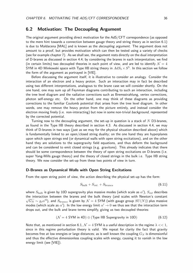
CHAPTER 6. MOTIVATING THE ADS/CFT CORRESPONDENCE 36
6.2 Motivation: The Decoupling Argument
The original argument providing direct motivation for the AdS/CFT correspondence (as opposedto the mere hint towards a connection between gauge theory and string theory as in section 6.1)is due to Maldacena [MAL] and is known as the decoupling argument. The argument does notamount to a proof, but provides motivation which can then be tested using a variety of checks(see for example chapter 7). As we shall see, the argument rests directly on the dual interpretationof D-branes as discussed in section 4.4; by considering the branes in each interpretation, we find(in certain limits) two decoupled theories in each point of view, and are led to identify N = 4SYM in 4D Minkowski space with Type IIB string theory in AdS5×S5. In this section we followthe form of the argument as portrayed in [VIE].
Before discussing the argument itself, it is illustrative to consider an analogy. Consider theinteraction of an electron and a heavy proton. Such an interaction may in fact be describedusing two different interpretations, analogous to the brane case we will consider shortly. On theone hand, one may sum up all Feynman diagrams contributing to such an interaction, includingthe tree level diagram and the radiative corrections such as Bremsstrahlung, vertex corrections,photon self-energy etc. On the other hand, one may think of these diagrams as providingcorrections to the familiar Coulomb potential that arises from the tree level diagram. In otherwords, one may remove the heavy proton from the picture entirely, and instead consider theelectron moving freely (i.e. non-interacting) but now in some non-trivial background, representedby the corrected potential.
Turning now to the decoupling argument, the set-up in question is a stack of N D3-branes,as found in the Type IIB theory described in section 4.3. As discussed in section 4.4, we maythink of D-branes in two ways (just as we may for the physical situation described above) whichis fundamentally linked to an open/closed string duality; on the one hand they are hyperplanesupon which open strings end (or dynamical walls with open string excitations), and on the otherhand they are solutions to the supergravity field equations, and thus deform the backgroundand can be considered to emit closed strings (e.g. gravitons). This already indicates that thereshould be some correspondence between the theory of open string excitations on D-branes (i.e.super Yang-Mills gauge theory) and the theory of closed strings in the bulk i.e. Type IIB stringtheory. We now consider the set-up from these two points of view in turn.
D-Branes as Dynamical Walls with Open String Excitations
From the open string point of view, the action describing the physical set-up has the form:
Sbulk + Sint. + Sbranes (6.11)
where Sbulk is given by 10D supergravity plus massive modes (which scale as α′), Sint describesthe interaction between the branes and the bulk theory (and scales with Newton’s constant√GN ∼ gsα
′2), and Sbranes is given by N = 4 SYM (with gauge group SU(N)) plus massivemodes (which scale as α′). In the low energy limit α′ → 0 we thus see that the interaction termdrops out, and the bulk and brane terms simplify, giving us two decoupled theories:
(N = 4 SYM in 4D)⊕ (Type IIB Supergravity in 10D) (6.12)
Note that, as mentioned in section 6.1, N = 4 SYM is a useful description in the regime λ << 1,since in this regime perturbation theory is valid. We repeat for clarity the fact that gravitybecomes free at low energies or large distances; as is well known the coupling GN is dimensionfuland thus the effective dimensionless coupling scales with energy, causing it to vanish in the lowenergy limit (see [VIE]).

CHAPTER 6. MOTIVATING THE ADS/CFT CORRESPONDENCE 37
D-Branes as Supergravity Solutions
In parallel to the proton/electron analogy discussed previously, we now no longer think of thebranes as physical objects, and instead look for solutions to the supergravity field equations thatdescribe a charged ‘heavy body’ and create some non-trivial background which closed stringspropagate in. In fact, we already discussed such solutions in section 4.4, which are given byequations (4.29)-(4.31). For convenience we express here the solution specifically for the case ofN D3-branes, focusing on the gravitational part which is given by:
ds2 =1√
1 + L4
y4
ηµνdxµdxν +
√1 +
L4
y4d~y2 (6.13)
where equation (4.31) gives L4 = gsN4πα′2. Note that the supergravity description is usefulwhen the curvature (which is set by the scale L) is large compared to the string length ls sinceotherwise string effects are important and cannot be ignored. The useful regime is thus given byL ∼
√α′(gsN)
14 ls ∼
√α′ and thus we require λ ≡ gsN 1. We thus see that this is the
opposite regime to which the gauge theory description is useful in.As discussed in section 4.4, in the limit y L (i.e. far away from the branes) the solution
becomes that of 10-dimensional flat Minkowski space, which is easy to see from (6.13) since√1 + L4/y4 → 1. Another interesting limit however, considered by Maldacena, is the near-
horizon limit y L (i.e. close to the branes). In this limit we have√
1 + L4/y4 → L2/y2 andthus the metric becomes:
ds2 → y2
L2ηµνdx
µdxν +L2
y2d~y2 (6.14)
Writing the 6-dimensional Euclidean metric in spherical coordinates as d~y2 = dy2 + y2dΩ25 we
have in the near-horizon limit:
ds2y→0 =
(y2
L2ηµνdx
µdxν +L2
y2dy2
)+ L2dΩ2
5 (6.15)
We recognise, using (5.15), that this is nothing but the metric for the product geometry AdS5×S5, where the corresponding radius for both parts of the geometry is L. The geometry near tothe branes is thus regular and highly symmetrical.
We saw that, from the open string point of view, there are two decoupled theories in thelow energy limit. As we shall see, a similar decoupling occurs in the present case. Note that,as discussed above, the metric (6.13) becomes flat at y → ∞ and thus the coordinate t is theproper time for an observer at infinity. In contrast, as is familiar from general relativity, theproper time elapsed for an observer at some other spacetime point is given by ∆τ =
√−gtt∆t,
and correspondingly the energies are related by E = 1/√−gttE∞. In particular, close to the
branes we have from (6.15) that E∞ = yE/L and thus, for fixed E, the energy as observed atinfinity goes to zero as y → 0. For an observer at infinity in this point of view, there are thustwo decoupled low energy regimes:
• 10-dimensional supergravity close to the observer, since gravity becomes free at low en-ergies/large distances.
• Full Type IIB string theory close to the branes (i.e. in the geometry AdS5×S5); everything(i.e. all strings) becomes a low energy effect close to the branes for an observer at infinity,and thus there is no restriction to low energy massless modes.

CHAPTER 6. MOTIVATING THE ADS/CFT CORRESPONDENCE 38
We thus have the two decoupled theories:
(Type IIB String theory on AdS5 × S5)⊕ (Type IIB Supergravity in 10D) (6.16)
Thus, we finally reach the celebrated AdS/CFT correspondence, by looking at (6.12) and(6.16) and noticing that we can ‘cross off’ Type IIB supergravity on either side and thus identify:
(Type IIB String theory on AdS5 × S5) ≡ (N = 4 SYM in 4D) (6.17)
The fact that D-branes have a dual interpretation has led us to identify these two theories as dualdescriptions of each other. Although not generally regarded as a proof (because of, for example,the subtleties to do with the various limits), the decoupling argument provides strong motivationfor the above correspondence.
6.3 Statement of the Correspondence
With the correspondence motivated we can now state it in its different forms; these differ in theirstrengths based on the conditions they impose on the various relevant parameters that appear inthe theories. The precise form of the correspondence is given as:
Type IIB string theory on AdS5 × S5 (both with radius L) with 5-form flux N and string cou-pling gs is equivalent/dual to 4-dimensional N = 4 SYM with gauge group SU(N) and couplingconstant gYM ,
where the couplings are identified in the following way:
gs = g2YM L4 = 4πgsNα
′2 (6.18)
(and one further identifies the axion expectation value with the instanton angle as 〈C〉 = θI[FRE]); the motivation for the second equation in (6.18) is clear from the previous section, andthe motivation for the first (in addition to the argument presented in section 6.1 concerning thelarge N limit of gauge theories) comes from the fact that the closed string coupling constantis the square of the open string coupling constant (see section 4.2). This is referred to as thestrong form of the correspondence as it is supposed to hold for all values of the coupling constantgs = g2
YM and all values of N . The strong form is extremely difficult to check however, namelybecause the theory of string quantization on general curved manifolds such as AdS5 × S5 isnot yet adequately developed. We will thus shortly state two progressively weaker forms of thecorrespondence which admit more tangible checks.
Before doing so however, it is instructive to make contact with the holographic nature of thecorrespondence alluded to previously. We saw in section 5.3 that AdS5 has a boundary given byMinkowski space R1,3, and we have now seen that on one side of the correspondence we haveN = 4 SYM in R1,3. Indeed, it is in fact possible to consider this gauge theory as living on theboundary of AdS5. We saw previously that rather than having branes at the origin, as in the openstring picture, we may replace them with AdS5×S5 space, whose Minkowski boundary will thenpatch onto the full solution. Clearly, in the open string picture, it must be the information of thebranes themselves that provides the boundary conditions for patching onto the full solution. Inthis manner it is then natural to identify the branes as being in some sense on the boundary ofAdS5, and thus the gauge theory (which lives on the branes) can be said to live on the boundaryof AdS5. This is the sense in which the correspondence is a holographic principle, since the5-dimensional dynamics of Type IIB theory (after compactification on S5) can be encoded in agauge theory living on the 4-dimensional boundary.

CHAPTER 6. MOTIVATING THE ADS/CFT CORRESPONDENCE 39
Returning now to stating the correspondence, we can state a slightly weaker form, which weshall call the t’Hooft form, by going to the t’Hooft limit. Thus, in this form of the correspondence,one claims the above equivalence with the added conditions that N → ∞, gYM → 0 andλ ≡ g2
YMN is fixed. On the gauge theory side this then corresponds to a perturbation theorytopological expansion in 1/N as we saw in section 6.1, and on the string theory side one hasclassical Type IIB string theory with small expansion parameter gs = λ/N , as we also describedin the same section; this form of the correspondence thus coincides (albeit in a more precisemanner) with that which the argument in section 6.1 pointed towards. Finally, we have the weakform of the correspondence which, after taking the t’Hooft limit, involves taking the large λlimit. On the gauge theory side we know from section 6.1 that this corresponds to the strongcoupling (i.e. non-perturbative) regime, whereas on the string theory side we have classical TypeIIB supergravity, with an expansion in small α′ (as is clear from (6.18)). Although the weakeststatement, this final form of the correspondence turns out to be extremely powerful, since onemay use classical gravity to perform calculations in non-perturbative gauge theory (see chapter7).
6.4 First Check: Correspondence of the Global Symmetries
The first check of the correspondence that we may perform, which is simple but necessary, isto map the global symmetries on the two sides of the correspondence. Luckily, we have alreadydone most of the work for this check in previous sections. We saw in section 3.3 that N = 4SYM has a global symmetry group given by the superconformal group SU(2, 2|4) which arosefrom the non-trivial combination of supersymmetry and conformal symmetry, together with theR-symmetry group SO(6)R ∼= SU(4)R. The bosonic subgroup of this supergroup is given bythe product of the conformal group and the R-symmetry group i.e. SO(2, 4)×SO(6)R. On thestring theory side we recognise this bosonic subgroup as the isometry group of the spacetimeAdS5×S5, since we saw in section 5.1 that the isometry group of AdSd is SO(2, d− 1) (and ofcourse the isometry group of S5 is SO(6)). Furthermore, as discussed in [FRE] although the D3-brane breaks precisely half of the Poincare supersymmetries (i.e. 16 of the 32), in the AdS5×S5
near-horizon limit, these are in fact supplemented by a further 16 conformal supersymmetries,enhancing the overall symmetry group to the full SU(2, 2|4) in correspondence with the fieldtheory side.
In addition to the global symmetry group SU(2, 2|4), we saw in section 3.2 that SYM alsohas the (conjectured) S-duality symmetry group SL(2,Z). However, we also saw in section 4.3that Type IIB string theory has an SL(2,R) symmetry that when quantized reduces to SL(2,Z),in accordance with the field theory side. This agreement only holds in the strongest form of thecorrespondence however, as it is only in this form that we have the full quantum Type IIB stringtheory. We thus see that, at the level of the global symmetries at least, the correspondence inits strongest form seems to be valid. We shall provide more thorough tests in the next chapter,though for weaker forms of the correspondence as these are easier to check.

Chapter 7
The Field/Operator Map and the Witten Prescription
In the previous chapter we saw the motivation of the original AdS/CFT correspondence due toMaldacena, as well as its statement in three forms of differing strength. We also saw a first basiccheck of the correspondence, which involved mapping the global symmetries of the theories onthe two sides of the correspondence. In this chapter we shall investigate the subject of testingthe correspondence in more detail. In particular, if the two theories are supposed to be dual, thenthere should be some mapping between the fundamental observables i.e. the fields/operators, aswell as the correlators. We shall thus provide such a field/operator map as well as a prescription,due to Witten, for mapping the correlators between the two theories; we well then discuss somesimple checks of the correspondence. We will be working in the classical supergravity limit andthus considering the weak form of the correspondence.
7.1 The Field/Operator Map
In section 6.4 we saw an agreement between the global symmetries on both sides of the cor-respondence. In addition to this it is important that there exists a correspondence betweenthe specific representations of the symmetry group that the observables of the two theories liein. In particular, we would like a correspondence between the supergravity fields in AdS5 andobservables in N = 4 SYM (which are the local gauge invariant operators described briefly insection 3.3). Consider a free massless scalar field φ in AdS5 × S5. The Kaluza-Klein procedureof dimensional reduction involves decomposing this field into a basis of 5-dimensional sphericalharmonics on S5 as (see [FRE]):
φ(x, y) =∑n
φn(x)Yn(y) (7.1)
where x are the AdS5 coordinates and y are the S5 coordinates. The equation of motion10φ = 0 on AdS5 × S5 then implies (5 + m2)φn = 0 for some mass m on AdS5. The 10-dimensional massless scalar fields, when compactified on S5, thus becomes massive scalar fieldson AdS5, with particular masses determined by the original action. We will see now that thismass is in fact related to the scaling dimension of the field, which allows for a correspondencebetween the scalar fields and the SYM observables (similar arguments hold for higher-spin fields,but we restrict the discussion to the simplest case of scalars).
We wish to study this 5-dimensional massive wave equation on AdS5. Let us in fact considergeneral Euclidean AdSd+1 space with unit radius for convenience (there are subtleties with theMinkowski case), in Poincare coordinates x = (x0, ~x) with metric analogous to (5.16) given by:
ds2 =dx2
0 + d~x2
x20
(7.2)
where d~x2 =∑d
i=1 dx2i . The Laplacian for a spacetime of metric gµν is given by [ZEE]:
= − 1√g∂µ√ggµν∂ν (7.3)
40

CHAPTER 7. THE FIELD/OPERATOR MAP AND THE WITTEN PRESCRIPTION 41
Using this together with the metric (7.2), for AdSd+1 one finds:
d+1 = −x20∂
20 + (d− 1)x0∂0 − x2
0
d∑i=1
∂2i (7.4)
We thus have the wave equation (d+1 +m2)φ = 0 with d+1 as in (7.4). Let us in particularassume solutions that asymptotically are eigenstates of dilatations in the x0-direction (this willbe important for the correspondence below); in other words, we assume solutions of the formφ(x) ∼ xk0 for some k. The wave equation then becomes:
−x20k(k − 1)xk−2
0 + (d− 1)x0kxk−10 − 0 +m2xk0 = 0 (7.5)
which implies the quadratic equation:
k2 − dk −m2 = 0 (7.6)
The solutions to this equation are found easily as:
k =d
2±
√(d
2
)2
+m2 (7.7)
and so such solutions to the wave equation are given by x∆0 and xd−∆
0 where:
∆ ≡ d
2+
√(d
2
)2
+m2 (7.8)
These are known as normalizable and non-normalizable modes respectively [FRE], so-calledbecause the latter are not square-integrable, whereas the former are. They are linearly indepen-dent modes, and describe the asymptotics at the boundary x0 → 0 of a general solution to thewave equation. A general solution then asymptotically has the form:
φ∆(x0, ~x) ∼ x∆0 f(~x) + xd−∆
0 g(~x) (7.9)
Recall from section 5.4 that AdS space in Poincare coordinates has a manifest dilatation isometry.Indeed, the metric (7.2) is invariant under the simultaneous scalings x0 → λx0 and ~x → λ~x.The scalar field φ∆ should be a representation of the isometry group and thus should be leftinvariant by this transformation. Given the form (7.9), we thus see that under this dilatation wemust have:
f(~x)→ λ−∆f(~x)
g(~x)→ λ∆−dg(~x)(7.10)
Recalling (2.23) we see that ∆ can thus be interpreted as a conformal dimension for the 4-dimensional field f(~x), and that g(~x) has a related dimension. This observation is crucial informing a map between observables in the AdS/CFT correspondence as we now discuss. Pluggingd = 4 into (7.8) for our case AdS5 we find the following relationship between mass and conformaldimension:
m2 = ∆(∆− 4) (7.11)
Since the representations (of the conformal group in SYM and the isometry group of AdS) onboth sides of the correspondence should match, we thus associate a field of mass m in AdS5 withan operator in SYM of conformal dimension ∆, where m and ∆ are related as in (7.11). The

CHAPTER 7. THE FIELD/OPERATOR MAP AND THE WITTEN PRESCRIPTION 42
correspondence is in fact more specific than this; as argued in [KRA], the non-normalizable modes(or, more specifically, their coefficients g(~x) in the solution (7.9)) correspond to sources for theassociated SYM operators, whereas the normalizable modes correspond to vacuum expectationvalues for the associated operators. Indeed, the normalizable modes define 4-dimensional fieldswith conformal dimension ∆, whereas the non-normalisable modes define a field g(~x) which isan appropriate source field for a CFT operator O of dimension ∆ since the coupling integral:∫
dd~xg(~x)O(~x) (7.12)
that appears in the exponent of the CFT generating functional is then invariant under dilatations:∫dd~xg(~x)O(~x)→
∫λddd~xλ∆−dg(~x)λ−∆O(~x) =
∫dd~xg(~x)O(~x) (7.13)
In particular, the non-normalizable modes define associated boundary fields which we now denoteas [FRE]:
φ∆(~x) ≡ limx0→0
φ∆(x0, ~x)x∆−40 (7.14)
These will be important in the following section.Although the above discussion has been for scalars, similar correspondences exist for higher-
spin fields. As discussed in [FRE], one finds that (7.11) also holds for spin-2 fields, and for otherspins one has the following relations between mass and conformal dimension:
Spin 1/2 and 3/2: |m| = ∆− 2
p-form: m2 = (∆− p)(∆ + p− 4)(7.15)
As an example we briefly mention that the supergravity modes (which include both a 5-dimensionalsupergravity multiplet plus an infinite tower of Kaluza-Klein modes obtained from compactifica-tion) correspond to SYM operators given by chiral primaries (such as the SO(6)-traceless partsof the single trace operators given in equation (3.19)) and their descendants; for example, thesupergravity multiplet defined by equation (3.20) is such a chiral primary (hence its name). Themassive Type IIB string modes however are given by non-chiral operators and their descendants,such as the Konishi multiplet Tr[XiXi] also introduced in (3.20). A complete mapping betweenSYM operators and the supergravity modes is provided in Table 7 of [FRE].
7.2 The Witten Prescription for Mapping Correlators
We saw in the previous section a correspondence between the fields on the supergravity sideand the operators on the SYM side of the correspondence. However, we would also like acorrespondence between the correlation functions on the two sides. Note that, since the field φ∆
has no gauge index, the associated operator O∆ should clearly be gauge invariant (the associatedoperator must thus be composite since the elementary fields in SYM all have gauge indices; seesection 3.2). Considering what we said in section 7.1 regarding non-normalizable modes asdefining sources for the associated operator, the SYM generating functional for operators O∆
then has the form [NAS]:
ZO[φ∆] =
∫D[SYM Fields]e−SSYM+
∫d4~xO∆(~x)φ∆(~x) (7.16)
which, upon differentiation with respect to φ∆(~x), gives correlation functions for the operatorsin the usual way:
〈O(~x1)...O(~xn)〉 =δn
δφ(~x1)...δφ(~xn)ZO[φ]|φ=0 (7.17)
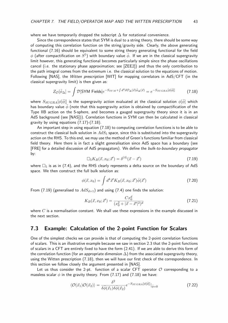
CHAPTER 7. THE FIELD/OPERATOR MAP AND THE WITTEN PRESCRIPTION 43
where we have temporarily dropped the subscript ∆ for notational convenience.Since the correspondence states that SYM is dual to a string theory, there should be some way
of computing this correlation function on the string/gravity side. Clearly, the above generatingfunctional (7.16) should be equivalent to some string theory generating functional for the fieldφ (after compactification on S5) with boundary value φ. If we are in the classical supergravitylimit however, this generating functional becomes particularly simple since the phase oscillationscancel (i.e. the stationary phase approximation; see [ZEE2]) and thus the only contribution tothe path integral comes from the extremum i.e. the classical solution to the equations of motion.Following [NAS], the Witten prescription [WIT] for mapping correlators in AdS/CFT (in theclassical supergravity limit) is then given as:
ZO[φ∆] =
∫D[SYM Fields]e−SSYM+
∫d4~xO∆(~x)φ∆(~x) = e−SSUGRA[φ[φ]] (7.18)
where SSUGRA[φ[φ]] is the supergravity action evaluated at the classical solution φ[φ] whichhas boundary value φ (note that this supergravity action is obtained by compactification of theType IIB action on the 5-sphere, and becomes a gauged supergravity theory since it is in anAdS background (see [NAS])). Correlation functions in SYM can then be calculated in classicalgravity by using equations (7.17)-(7.18).
An important step in using equation (7.18) to computing correlation functions is to be able toconstruct the classical bulk solution in AdS5 space, since this is substituted into the supergravityaction on the RHS. To this end, we may use the method of Green’s functions familiar from classicalfield theory. Here there is in fact a slight generalisation since AdS space has a boundary (see[FRE] for a detailed discussion of AdS propagators). We define the bulk-to-boundary propagatorby:
5KB(~x, x0; ~x′) = δ(4)(~x− ~x′) (7.19)
where 5 is as in (7.4), and the RHS clearly represents a delta source on the boundary of AdSspace. We then construct the full bulk solution as:
φ(~x, x0) =
∫d4~x′KB(~x, x0; ~x′)φ(~x′) (7.20)
From (7.19) (generalised to AdSd+1) and using (7.4) one finds the solution:
KB(~x, x0; ~x′) =Cxd0
(x20 + |~x− ~x′|2)d
(7.21)
where C is a normalisation constant. We shall use these expressions in the example discussed inthe next section.
7.3 Example: Calculation of the 2-point Function for Scalars
One of the simplest checks we can provide is that of computing the 2-point correlation functionsof scalars. This is an illustrative example because we saw in section 2.3 that the 2-point functionsof scalars in a CFT are entirely fixed to have the form (2.41). If we are able to derive this form ofthe correlation function (for an appropriate dimension ∆) from the associated supergravity theory,using the Witten prescription (7.18), then we will have our first check of the correspondence. Inthis section we follow closely the argument presented in [NAS].
Let us thus consider the 2-pt. function of a scalar CFT operator O corresponding to amassless scalar φ in the gravity theory. From (7.17) and (7.18) we have:
〈O(~x1)O(~x2)〉 =δ2
δφ(~x1)δφ(~x2)e−SSUGRA[φ[φ]]|φ=0 (7.22)

CHAPTER 7. THE FIELD/OPERATOR MAP AND THE WITTEN PRESCRIPTION 44
The 5-dimensional supergravity action, after using (7.20), has the following schematic scalar fieldcontribution:
SSUGRA[φ[φ]] ∼∫d5x√g
∫d4~x′d4~y′∇µKB(~x, x0; ~x′)φ(~x′)∇µKB(~x, x0; ~y′)φ(~y′) +O(φ3)
(7.23)where, schematically, ∇µ∇µ ≡ 5 is the kinetic operator. From (7.23) we see clearly that:
SSUGRA[φ[φ]]|φ=0 =δSSUGRA[φ[φ]]
δφ|φ=0 = 0 (7.24)
since all terms include at least two fields φ, and thus non-zero contributions begin at secondorder derivatives, giving (abbreviating the action as S for convenience):
〈O(~x1)O(~x2)〉 =δ
δφ(~x1)
(− δS
δφ(~x2)e−S
)|φ=0 = − δ2S
δφ(~x1)δφ(~x2)|φ=0 (7.25)
For the 2-point functions we may thus ignore the interaction terms implicit in (7.23), since wetake only 2 derivatives before setting φ0 = 0; this greatly simplifies the problem, and only appliesto the computation of the 2-point function (and not, for example, to the computation we shalldiscuss in section 7.4). We can thus effectively consider a free massless scalar field with equationof motion 5φ = 0 and action given by the usual expression:
S =1
2
∫d5x√g∂µφ∂
µφ (7.26)
which upon integration by parts and using the equation of motion to kill one term becomes:
S =1
2
∫d5x√g∂µ(φ∂µφ) =
1
2
∫boundary
d4~x√h(φ~n · ∇φ) (7.27)
where h is the metric on the boundary, and ~n · ∇ is the component of the gradient normal tothe boundary.
Let us unpack each of the terms on the RHS of equation (7.27) individually before taking theboundary limit x0 → 0 of the full expression. Since the boundary is defined by a slice of constantx0, from (7.2) we thus have
√h = x−d0 and ~n · ∇ = x0∂/∂x0. From (7.27), we see that we
also need to investigate φ~n · ∇φ = φx0∂φ/∂x0 at the boundary. Clearly, by construction, in thislimit we let the scalar field become its associated boundary value i.e. φ(~x, x0) → φ(~x). Notethat from (7.20) we have:
x0∂φ
∂x0(~x, x0) = x0
∫dd~x′
∂KB
∂x0(~x, x0; ~x′)φ(~x′) (7.28)
and furthermore from (7.21) we have:
∂KB
∂x0(~x, x0; ~x′) =
dCxd−10
(x20 + |~x− ~x′|2)d
− dC2xd+10
(x20 + |~x− ~x′|2)d+1
(7.29)
In the limit x0 → 0, the factors of x0 in the denominators in (7.29) become negligible, andfurthermore xd+1
0 → 0 faster than xd−10 does. The first term is thus clearly dominant, and we
have:
x0∂KB
∂x0(~x, x0; ~x′)→x0→0
dCxd0|~x− ~x′|2d
(7.30)
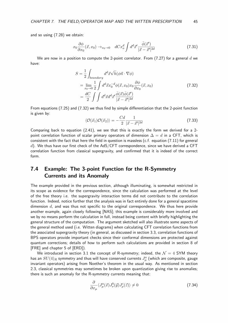
CHAPTER 7. THE FIELD/OPERATOR MAP AND THE WITTEN PRESCRIPTION 45
and so using (7.28) we obtain:
x0∂φ
∂x0(~x, x0)→x0→0 dCxdo
∫dd~x′
φ(~x′)
|~x− ~x′|2d(7.31)
We are now in a position to compute the 2-point correlator. From (7.27) for a general d wehave:
S =1
2
∫boundary
dd~x√h(φ~n · ∇φ)
= limx0→0
1
2
∫dd~xx−d0 φ(~x, x0)x0
∂φ
∂x0(~x, x0)
=dC
2
∫ ∫dd~xdd~x′
φ(~x)φ(~x′)
|~x− ~x′|2d
(7.32)
From equations (7.25) and (7.32) we thus find by simple differentiation that the 2-point functionis given by:
〈O(~x1)O(~x2)〉 = −Cd2
1
|~x− ~x′|2d(7.33)
Comparing back to equation (2.41), we see that this is exactly the form we derived for a 2-point correlation function of scalar primary operators of dimension ∆ = d in a CFT, which isconsistent with the fact that here the field in question is massless (c.f. equation (7.11) for generald). We thus have our first check of the AdS/CFT correspondence, since we have derived a CFTcorrelation function from classical supergravity, and confirmed that it is indeed of the correctform.
7.4 Example: The 3-point Function for the R-SymmetryCurrents and its Anomaly
The example provided in the previous section, although illuminating, is somewhat restricted inits scope as evidence for the correspondence, since the calculation was performed at the levelof the free theory i.e. the supergravity interaction terms did not contribute to the correlationfunction. Indeed, notice further that the analysis was in fact entirely done for a general spacetimedimension d, and was thus not specific to the original correspondence. We thus here provideanother example, again closely following [NAS]; this example is considerably more involved andwe by no means perform the calculation in full, instead being content with briefly highlighting thegeneral structure of the computation. The argument sketched will also illustrate some aspects ofthe general method used (i.e. Witten diagrams) when calculating CFT correlation functions fromthe associated supergravity theory (in general, as discussed in section 3.3, correlation functions ofBPS operators provide important checks since their conformal dimensions are protected againstquantum corrections; details of how to perform such calculations are provided in section 8 of[FRE] and chapter 5 of [ERD]).
We introduced in section 3.1 the concept of R-symmetry; indeed, the N = 4 SYM theoryhas an SU(4)R symmetry and thus will have conserved currents Jaµ (which are composite, gaugeinvariant operators) arising from Noether’s theorem in the usual way. As mentioned in section2.3, classical symmetries may sometimes be broken upon quantization giving rise to anomalies;there is such an anomaly for the R-symmetry currents meaning that:
∂
∂xµ〈Jaµ(~x)Jbν(~y)Jcρ(~z)〉 6= 0 (7.34)

CHAPTER 7. THE FIELD/OPERATOR MAP AND THE WITTEN PRESCRIPTION 46
and this anomaly is antisymmetric in µ, ν, ρ and appears at 1-loop order only, meaning that it canbe calculated exactly i.e. it is an unrenormalised quantity. This is extremely useful as it allowsthe computation of the anomaly from the AdS side to be directly compared to the known answercomputed using CFT (recall the importance of unrenormalised quantities, due to the fact thatthe classical supergravity regime is the strong-coupling regime on the gauge side as discussed insections 6.2 and 6.3).
From the Witten prescription we know that the composite, gauge-invariant R-currents Jaµwill couple to the non-renormalisable modes of some associated supergravity field, and from theindex structure this will have the form Aaµ, with associated boundary value Aaµ. We know thata is an R-symmetry index in the algebra SU(4) ∼= SO(6); it turns out that on the supergravityside the fields Aaµ are then the gauge fields of the 5-dimensional gauged supergravity obtainedby compactification of Type IIB supergravity on S5 (with isometry group SO(6)). The Wittenprescription, analogous to (7.18), then states the following:
ZJ [A] =
∫D[SYM Fields]e−SSYM+
∫d4~xJaµ(~x)Aaµ(~x) = e−SSUGRA[A[A]] (7.35)
where, again, on the RHS one substitutes the classical solution A[A] in SSUGRA with boundaryvalue A. In analogy to (7.22) and (7.25) one then has:
〈Jaµ(~x)Jbν(~y)Jcρ(~z)〉 =δ3e−SSUGRA[A[A]]
δAaµ(~x)δAbν(~y)δAcρ(~z)|A=0 = − δ3SSUGRA[A[A]]
δAaµ(~x)δAbν(~y)δAcρ(~z)|A=0 (7.36)
The bulk solution is then given in terms of the boundary value via the bulk-to-boundary propagatoras in (7.20):
Aaµ(~x, x0) =
∫d4~x′Gµα(~x, x0; ~x′)Aaα(~x′) (7.37)
except now the bulk-to-boundary propagator Gµα is gauge-dependent since Aaµ is (in actuallydoing the calculations it is useful to choose a bulk-to-boundary propagator that is conformal onthe boundary).
Given (7.36)-(7.37), we see that for the 3-point function we are only interested in termsin SSUGRA that are cubic in the gauge field. The 5-dimensional supergravity action has thefollowing schematic form for Aµ [NAS]:
SSUGRA|Aµ ∼∫ [
(A)2 term + (AaµAbνA
cρ) term + ...
](7.38)
where the quadratic term determines the propagator, and one may then perform classical per-turbation theory in the interaction terms using tree-level diagrams known as Witten diagrams(the restriction to tree-level comes from the fact that we are in the classical limit; loops wouldcorrespond to quantum corrections). Witten diagrams are essentially tree-level Feynman dia-grams, but there is an extra feature present due to the fact that AdS space has a boundary;the bulk of the spacetime is then represented as a disc, with the outer circle representing theboundary of the space. Propagators are then represented as usual by lines (and may be eitherbulk-to-bulk, bulk-to-boundary, or boundary-to-boundary), and the vertex factors are determinedin the usual way from the supergravity action. As an example, the only diagram that contributesto the calculation of the 3-point function in question is given in Figure 7.1, which consists of 3bulk-to-boundary propagators and a single 3-point vertex.
Let us consider specifically the anomaly of the 3-point function. In addition to a term thatis cubic in the gauge fields, the contribution from the action should also be antisymmetric in thespacetime indices, since we mentioned previously that the anomaly has these properties. Such

CHAPTER 7. THE FIELD/OPERATOR MAP AND THE WITTEN PRESCRIPTION 47
~x ~y
~z
Figure 7.1: Witten diagram contributing to the 3-point R-current function.
a term does appear in the 5-dimensional supergravity action and is known as the Chern-Simonsterm which has the form:
SCS(A) =iN2
16π2Tr
∫d5xεµνρστ (Aµ(∂νAρ)∂σAτ + ...) (7.39)
One can determine the R-current anomaly from the gravity side rather neatly in the followingway. Under a gauge transformation δAaµ = (DµΛ)a = ∂µΛa + gYMf
abcA
bµΛc (where fabc are the
structure constants of the gauge group) one finds (see [NAS] for all details):
δΛSCS = − iN2
16π2dabc
∫boundary
d4xεµνρσΛa∂µ
(Abν∂ρA
cσ +
1
4f cdeA
bνA
dρA
eσ
)(7.40)
where dabc = Tr(TaTb, Tc), and since the integral is performed on the boundary we may replaceA→ A throughout. However, from the Witten prescription (7.35) we also have:
δΛSSUGRA[A[A]] = δΛ(−lnZ[A]) =
∫d4xδAµa(x)Jaµ(x) = −
∫d4xΛa(DµJµ)a (7.41)
and thus by comparison one finds the following operator equation for the covariant derivative ofthe R-symmetry current:
(DµJµ)a(x) =iN2
16π2dabcε
µνρσ∂µ
(Abν∂ρA
cσ +
1
4f cdeA
bνA
dρA
eσ
)(7.42)
It turns out that this agrees exactly with the CFT 1-loop anomaly computation (given via (7.34)),thus confirming the validity of the correspondence in this case.
In addition to the anomalous part, one may proceed to compute the full 3-point function usingthe method sketchily laid out in this section, and proceeding roughly in a similar fashion to the 2-point function calculation done previously (though in the present case the supergravity interactionterms cannot all be ignored). After some work (again see [NAS] for details), one finds that thefunction has the correct spacetime dependence for a CFT 3-point function, and furthermoreagrees exactly with the result one obtains at 1-loop order in the CFT computation. This latterresult is perhaps somewhat surprising, since we mentioned previously that the supergravity limiton the string theory side corresponds to the strong-coupling regime on the gauge theory side;we would thus not expect the supergravity result to precisely agree with the result one obtainsfrom the lower orders of CFT perturbation theory. Clearly then, for the above to be true, theremust be a non-renormalisation theorem which means that the full 3-point function (not just theanomaly) is in fact 1-loop exact; as discussed in [NAS], such a theorem was indeed proven, using

CHAPTER 7. THE FIELD/OPERATOR MAP AND THE WITTEN PRESCRIPTION 48
the superconformal symmetry of the theory. We have thus seen another check of the AdS/CFTcorrespondence, and indeed one that is more powerful than that in the previous section, sincethe current check is performed at the level of the full interacting theory. There is, however,a limit to how far the scope of these tests extends related to the fact that they are based onunrenormalised quantities; we shall briefly discuss this issue in section 8.2.

Part III
Conclusion: Beyond the OriginalConjecture
49

Chapter 8
Conclusion
8.1 Extensions of the Correspondence
In this dissertation we have been primarily concerned with the original AdS/CFT correspondencedue to Maldacena, relating Type IIB theory on AdS5 × S5 to N = 4 SYM. This required con-siderable background since we saw, for example, that the gauge theory in the correspondenceis both supersymmetric and conformal, leading to a larger superconformal symmetry (which wementioned has special representations of particular importance in testing the correspondence).These need not be general features of a gauge/gravity duality however. Indeed, the originalcorrespondence has been extended to other cases containing, for example, less supersymmetryand/or no conformal symmetry on the gauge theory side. The original correspondence is par-ticularly powerful since the high levels of symmetry available allow numerous computations tobe performed. Conceptually, however, it is fairly remote from the gauge theories we see in na-ture, which seem to be neither supersymmetric nor conformal. These extensions of the originalcorrespondence are thus important, and are being continually studied in the field.
Before briefly mentioning such examples however, we note that there are in fact other caseswhich relate a string theory in an AdS background to a gauge theory with conformal symmetryand maximal supersymmetry, much like the original correspondence. The string theory in questionis now the somewhat elusive M-theory which, although not very well understood, is known tohave as its low energy limit the D = 11 supergravity theory. In the same way that AdS5×S5 aroseas the near-horizon limit to a stack of D3 branes, the maximally supersymmetric backgroundsfor D = 11 supergravity given by AdS4 × S7 and AdS7 × S4 can be seen to arise from branesolutions known as M2 and M5-branes. Indeed, in a similar fashion to the decoupling argumentdiscussed in chapter 6, Maldacena motivated [MAL] that M-theory in these backgrounds is infact dual to particular conformal field theories in 3 and 6-dimensions respectively.
Furthermore, there is a class of correspondences relating a string theory in the backgroundAdSd+1×X (for some space X) to a gauge theory in d-dimensions with conformal symmetry butless than maximal supersymmetry. Indeed, recall from section 6.4 that the presence of an AdSbackground relates to the presence of conformal symmetry in the gauge theory, since the isometrygroup of AdSd+1 is the conformal group in R1,d−1. Furthermore, we saw that for X = S5 theisometry group was equivalent to the R-symmetry group of the gauge theory, which is directlyrelated to the degree of supersymmetry N (see section 3.1). We thus see that we can modify thedegree of supersymmetry by modifying this space X. For example, by starting with a maximallysupersymmetric theory, we may divide the corresponding space X by some discrete subgroup,thereby reducing its isometry group and thus reducing the number of supersymmetries on thegauge theory side (more details and an example of such a correspondence are provided in [NAS]).In this manner we may produce correspondences with less supersymmetry on the gauge theoryside, as is important for the reasons mentioned previously. Such cases may be tested in similarways to those described in chapter 7 for the original correspondence, though generally fewer testsare possible since the presence of less symmetry means that fewer quantities are protected againstquantum corrections. It is also possible to break the conformal invariance of the gauge theory,
50

CHAPTER 8. CONCLUSION 51
which is important for practical applications. This may be achieved, for example, by consideringthe gauge theory at finite temperature; the introduction of a temperature sets an energy scaleand thus breaks the scale (and thus conformal) invariance of the theory. The energy scale of thegauge theory then becomes significant since the theory is no longer conformal, and is identifiedwith the additional dimension on the gravity side (see [NAS]) e.g. the radial dimension x0 or rfor AdSd defined in section 5.4. It turns out that the UV regime of the gauge theory correspondsto the IR (or large distances) regime of the gravity dual, leading to what is sometimes known asthe UV-IR correspondence.
We briefly summarise some general properties of gauge/gravity dualities relevant to the as-pects we have discussed in the present dissertation (a more complete mapping is provided in[NAS]). First, the gauge group (which in addition to SU(N) may be other groups such asSO(N) or Sp(N)) has no analogue in the gravity theory (e.g. SU(N) in the original corre-spondence does not appear on the gravity side); indeed, only gauge invariant observables can becalculated, such as the correlation functions of gauge invariant operators discussed previously.Second, the global symmetries of the gauge theory (e.g. the R-symmetry of N = 4 SYM) corre-spond to gauge symmetries in the compactified gravity theory (e.g. the gauged supergravity oneobtains from compactifying Type IIB on S5); the Noether currents in the former then couple tothe gauge fields in the latter, as in the example we saw in section 7.4 (in general, the gravityfields correspond and couple to some gauge invariant operators in the gauge theory, similar tothat in section 7.1). Finally, the couplings are always related by gs ≡ g2
g where gg is the gaugetheory coupling; this fundamentally arises from the fact that the closed string coupling constantis the square of the open string coupling constant, as discussed in section 4.2. We see that thereare thus many structural similarities between different gauge/gravity dualities.
8.2 Closing Remarks
The AdS/CFT correspondence is a continuously growing field of active research. We have seen insome detail how the original correspondence is motivated and formulated, and described how testsof the correspondence are possible. There is however a subtle point worth mentioning regardingthese tests as alluded to at the end of chapter 7. The tests we have predominantly describedinvolve unrenormalised quantities on the gauge theory side, which are important since they allowfor computations in the CFT that can be compared with the results obtained from the associatedgravity theory. However, there is some debate concerning how deep the evidence that these testsprovide for the correspondence really runs, since the results are essentially consequences of thesymmetries (which we have already checked agree on the two sides) and so do not necessarilyprove that the dynamics of the two theories are equivalent in a non-trivial way. There hashowever been much work in attempting to provide non-trivial checks of the correspondence atthe dynamical level, for example by studying integrability in AdS/CFT (see [INT]) and gauge-invariant quantities known as Wilson loops (see [GRO] for example). Many such checks haveindeed been performed in the literature, providing strong evidence for the conjecture, even if it isyet to be fully proven in a rigorous manner. We have also briefly seen how the correspondence canbe extended to other cases; some of these, for example, are of particular interest in applicationsto condensed matter physics and the study of realistic gauge theories. In addition to theseapplications, it is of course also of great conceptual interest that the bulk gravitational degreesof freedom may be encoded in a boundary theory via holography; this is an idea that has capturedscientists and philosophers alike, and is likely to be one that will be investigated for sometime.

References
[MAL] “The Large N Limit of Superconformal Field Theories and Supergravity”. Maldacena.Adv.Theor.Math.Phys.2:231-252. [arXiv:hep-th/9711200] (1997).
[BEK] “Black Holes and Entropy”. Bekenstein. Physical Review D 7(8):2333 (1973).
[STR] “The dS/CFT Correspondence”. Strominger. JHEP 0110:034. [arXiv:hep-th/0106113](2001).
[HAR] “Horizons, holography and condensed matter”. Hartnoll. [arXiv:1106.4324] (2011).
[GOM] “Lectures on Conformal Field Theory”. http://www.perimeterscholars.org/327.html.Gomis. Perimeter Institute (2011).
[ERD] “Introduction to gauge gravity duality”. Erdmenger (2010).
[PES] “An Introduction to Quantum Field Theory”. Peskin and Schroeder. Westview Press(1995).
[COL] “All Possible Symmetries of the S Matrix”. Coleman and Mandula. Physical Review159 (5): 12511256 (1967).
[BAL] “Supersymmetric Gauge Field Theory and String Theory”. Balin and Love. Taylor andFrancis (1994).
[FRE] “Supersymmetric Gauge Theories and the AdS/CFT Correspondence”. Freedman andd’Hoker. [arXiv:hep-th/0201253] (2002).
[ZHO] “Group Theory for Physicists”. Zhong-Qi Ma. World Scientific (2007).
[KIR] “String Theory in a Nutshell”. Kiritsis. Princeton University Press (2007).
[MON] C. Montonen and D. Olive, Phys. Lett. B72 (1977).
[POL] “String Theory, Vol. 1 ”. Polchinski. Cambridge University Press (2005).
[CAC] “Lectures on String Theory”. http://www.perimeterscholars.org/337.html. Cachazo.Perimeter Institute (2011).
[ZWE] “A First Course in String Theory, Second Edition”. Zweibach. Cambridge UniversityPress (2009).
52

CHAPTER 8. CONCLUSION 53
[FRA] “The Geometry of Physics, an Introduction, Second Edition”. Frankel. Cambridge Uni-versity Press (2004).
[VIE] “Lectures on Explorations in String Theory”. http://www.perimeterscholars.org/341.html.Vieira. Perimeter Institute (2011).
[NAK] “Geometry, Topology and Physics, Second Edition”. Nakahara. Taylor and Francis (2003).
[ZEE] “Einstein Gravity in a Nutshell”. Zee. Princeton University Press (2013).
[ZEE2] “Quantum Field Theory in a Nutshell, 2nd Edition”. Zee. Princeton University Press(2010).
[KRA] “Spacetime and the holographic renormalization group”. Balasubramanian and Kraus.Phys. Rev. Lett. 83, 3605. [arXiv:hep-th/9903190] (1999)
[NAS] “Introduction to AdS-CFT”. Nastase. arXiv:0712.0689 (2007).
[WIT] “Anti De Sitter Space And Holography”. Witten. Adv. Theor. Math. Phys. 2 253-291, [hep-th/9802150] (1998).
[INT] “Review of AdS/CFT Integrability: An Overview”. Lett. Math. Phys. 99, 3. arXiv:1012.3982[hep-th] (2012).
[GRO] “An exact prediction of N = 4 SUSYM theory for string theory”. Gross and Drukker. J.Math. Phys. 42, 2896. [arXiv:hep-th/0010274] (2001).
Related Documents