EURASIP Journal on Image and Video Processing Johnston and Chazal EURASIP Journal on Image and Video Processing (2018) 2018:86 https://doi.org/10.1186/s13640-018-0324-4 REVIEW Open Access A review of image-based automatic facial landmark identification techniques Benjamin Johnston 1,2* and Philip de Chazal 1 Abstract The accurate identification of landmarks within facial images is an important step in the completion of a number of higher-order computer vision tasks such as facial recognition and facial expression analysis. While being an intuitive and simple task for human vision, it has taken decades of research, an increase in the availability of quality data sets, and a dramatic improvement in computational processing power to achieve near-human accuracy in landmark localisation. The intent of this paper is to provide a review of the current facial landmarking literature, outlining the significant progress that has been made in the field from classical generative methods to more modern techniques such as sophisticated deep neural network architectures. This review considers a generalised facial landmarking problem and provides experimental examples for each stage in the process, reporting repeatable benchmarks across a number of publicly available datasets and linking the results of these examples to the recently reported performance in the literature. Keywords: Face, Landmarking, Registration, Image, Vision, Machine learning, Deep learning, Artificial neural networks, Review, Survey 1 Introduction The accurate identification of specific facial features and landmarks is a foundational process by which a number of more complicated image analysis problems are solved. Tasks such as facial identification, expression analysis, age estimation, and gender classification are often built upon a facial landmarking component in their methods [1, 2]. The use of image-based automated facial landmarking has been extended outside of the domain of image research and into other applications, including some within the medical field. Conditions such as facial palsy, facial paral- ysis, and even sleep apnoea are either characterised by or associated with unique facial structures that enables the use of facial landmarking as a useful research or even screening tool. Very recently, Guarin et al. [3] described an automated facial landmarking tool which is used in the characterisation of facial displacements in sufferers of facial palsy; while the work by Anping et al. [4] uses land- marks as predicted by Active Shape Models to assess facial *Correspondence: [email protected] 1 Sleep Research Group, Charles Perkins Centre, School of Electrical and Information Engineering, 2006 University of Sydney, Sydney, NSW, Australia 2 ResMed Ltd, 1 Elizabeth Macarthur Dr, 2153 Bella Vista, NSW, Australia nerve paralysis. The use of facial landmarking methodolo- gies has been recently examined as a means of screening for sleep apnoea by Tabatabaei Balaei et al. [5], looking at the association between the underlying structure of pre- dicted facial landmarks and the likelihood of suffering from obstructive sleep apnoea. The authors of this review have also investigated the use of facial landmarks in sizing sleep apnoea masks [6], a critical device in sleep apnoea treatment. Given the wide variety of applications in which facial landmarking is applied, and in the case of medi- cal applications the critical nature of the tasks it is vital that the systems be capable of accurately identifying the landmarks of interest. While the process of identifying features such as the cor- ner of an eye on a face is a natural and instinctive task for human vision; it has proven somewhat more challeng- ing for computer vision, which has not benefited from millenia of evolution. Despite the overall similarity in the general content of facial images, common differences such as variation in pose, lighting, facial expression, and varia- tions in the facial features themselves can be problematic for many computer vision systems leading to significant errors in landmarking accuracy. © The Author(s). 2018 Open Access This article is distributed under the terms of the Creative Commons Attribution 4.0 International License (http://creativecommons.org/licenses/by/4.0/), which permits unrestricted use, distribution, and reproduction in any medium, provided you give appropriate credit to the original author(s) and the source, provide a link to the Creative Commons license, and indicate if changes were made.

Welcome message from author
This document is posted to help you gain knowledge. Please leave a comment to let me know what you think about it! Share it to your friends and learn new things together.
Transcript
EURASIP Journal on Imageand Video Processing
Johnston and Chazal EURASIP Journal on Image and VideoProcessing (2018) 2018:86 https://doi.org/10.1186/s13640-018-0324-4
REVIEW Open Access
A review of image-based automatic faciallandmark identification techniquesBenjamin Johnston1,2* and Philip de Chazal1
Abstract
The accurate identification of landmarks within facial images is an important step in the completion of a number ofhigher-order computer vision tasks such as facial recognition and facial expression analysis. While being an intuitiveand simple task for human vision, it has taken decades of research, an increase in the availability of quality data sets,and a dramatic improvement in computational processing power to achieve near-human accuracy in landmarklocalisation. The intent of this paper is to provide a review of the current facial landmarking literature, outlining thesignificant progress that has been made in the field from classical generative methods to more modern techniquessuch as sophisticated deep neural network architectures. This review considers a generalised facial landmarkingproblem and provides experimental examples for each stage in the process, reporting repeatable benchmarks acrossa number of publicly available datasets and linking the results of these examples to the recently reportedperformance in the literature.
Keywords: Face, Landmarking, Registration, Image, Vision, Machine learning, Deep learning, Artificial neuralnetworks, Review, Survey
1 IntroductionThe accurate identification of specific facial features andlandmarks is a foundational process by which a numberof more complicated image analysis problems are solved.Tasks such as facial identification, expression analysis, ageestimation, and gender classification are often built upona facial landmarking component in their methods [1, 2].The use of image-based automated facial landmarking hasbeen extended outside of the domain of image researchand into other applications, including some within themedical field. Conditions such as facial palsy, facial paral-ysis, and even sleep apnoea are either characterised byor associated with unique facial structures that enablesthe use of facial landmarking as a useful research or evenscreening tool. Very recently, Guarin et al. [3] describedan automated facial landmarking tool which is used inthe characterisation of facial displacements in sufferers offacial palsy; while the work by Anping et al. [4] uses land-marks as predicted by Active ShapeModels to assess facial
*Correspondence: [email protected] Research Group, Charles Perkins Centre, School of Electrical andInformation Engineering, 2006 University of Sydney, Sydney, NSW, Australia2ResMed Ltd, 1 Elizabeth Macarthur Dr, 2153 Bella Vista, NSW, Australia
nerve paralysis. The use of facial landmarking methodolo-gies has been recently examined as a means of screeningfor sleep apnoea by Tabatabaei Balaei et al. [5], looking atthe association between the underlying structure of pre-dicted facial landmarks and the likelihood of sufferingfrom obstructive sleep apnoea. The authors of this reviewhave also investigated the use of facial landmarks in sizingsleep apnoea masks [6], a critical device in sleep apnoeatreatment. Given the wide variety of applications in whichfacial landmarking is applied, and in the case of medi-cal applications the critical nature of the tasks it is vitalthat the systems be capable of accurately identifying thelandmarks of interest.While the process of identifying features such as the cor-
ner of an eye on a face is a natural and instinctive taskfor human vision; it has proven somewhat more challeng-ing for computer vision, which has not benefited frommillenia of evolution. Despite the overall similarity in thegeneral content of facial images, common differences suchas variation in pose, lighting, facial expression, and varia-tions in the facial features themselves can be problematicfor many computer vision systems leading to significanterrors in landmarking accuracy.
© The Author(s). 2018 Open Access This article is distributed under the terms of the Creative Commons Attribution 4.0International License (http://creativecommons.org/licenses/by/4.0/), which permits unrestricted use, distribution, andreproduction in any medium, provided you give appropriate credit to the original author(s) and the source, provide a link to theCreative Commons license, and indicate if changes were made.
Johnston and Chazal EURASIP Journal on Image and Video Processing (2018) 2018:86 Page 2 of 23
The intent of this paper is to review the current stateof automated image-based facial landmarking processesand provide a comparison of the performance achievedby some of these methods. This paper aims to build uponthe comprehensive review completed by Çeliktutan et al.[7]. Since the publication of this article in 2013 increasesin computing power through the reduction in the cost ofGPUs, in addition to an increase in the availability of largedatasets has enabled the development of highly accurate,though computationally expensive methods. While notcovered within this review, readers may also be interestedin the automated detection of facial landmarks in three-dimensional models. With the improved availability andreduced cost of three dimensional scanners such as theKinect or even those found in late model smartphones, 3Dfacial models are more readily available for analysis. Whilein some respects, automated 3D facial landmarking hasevolved from its 2D counterpart, significant differencesexist in the current focus of research. Three-dimensionallandmarking currently uses a series of powerful geometricdescriptors to both interpret and summarises the complexinformation encoded within the 3D model. Marcolin andVezzetti describe 105 novel descriptors [8] mapped on 217facial depth maps to generate a set of landmarks withina number of different facial expressions. Similar descrip-tors used by Vezzetti et al. in 2017 [9] achieved a meanlocalization error of 4.75 mm in facial scans containingdiffering emotions as well as the presence of occlusions,such as fingers or hands covering the face.The structure of this review will differ somewhat to pre-
vious image processing surveys. This discussion will occurwithin the framework of a generic process for construct-ing an automated facial landmarking model; reviewing thestate of the art at each stage of model construction. Thedetails of this structure will be outlined in more detail inthe next section; however, it is intended that reviewing theliterature in the framework of a generic process will pro-vide the reader with more clarity of the progress that hasbeen made within the field. To further support the review,stages 2, 3, and 4 also contain experimental componentswith the intent of improving reader understanding of thecorresponding stage. For a high performing, automatedlandmarking algorithm, it is important that each stagein constructing an automated methodology be carefullyconsidered and appropriate design choices made. By dis-cussing the state of the art within the context of thesestages, the authors hope the reader is able to more com-pletely understand the current state of the art.
2 Review2.1 Generic model constructionWhile there are many differences between the variousapplications and methods of automated facial landmark-ing, it is possible to describe a generic process by which
almost all models are created. This process which isnot necessarily unique to facial landmarking provides aneffective means for comparing different methodologies.We will define the generic model construction process ascomprising five stages:
1 Definition of the objective: what is the exact natureof the problem to be solved?,
2 Selection of an appropriate dataset for solving thedefined problem: what information is required tomeet the objective?,
3 Extraction of regions of interest from the dataset:what features from the selected dataset will best meetthe defined objective?,
4 Definition of model architecture: which model willgive the best performance? and
5 Model training and evaluation: what is the besttraining methodology given all of the above stage?
Each of the following sections will discuss in detail eachstage of the generic model construction process.
2.2 Stage 1: objective definitionThe objective definition is arguably the most importantstep in the model construction process. A clear, con-cise, and correct definition of what is to be achieved iscrucial as it forms the basis of all other steps, design deci-sions, and is often a platform for solving more complexproblems. Wu et al. in 2012 [1] used facial landmarksto assist in age estimation and face verification; Devrieset al. [2] used landmarking in facial expression recognitionwhile Tabatabaei Balaei et al. [5] investigated the use offacial landmarks as a means of determining the likelihoodthat an individual sufferer from obstructive sleep apnoea(OSA).This review paper will not consider any higher level
applications and will define the objective definition forthe generic model construction process as
Aiming to construct an automatic facial landmarkingsystem with performance comparable to that of anexpert human annotator
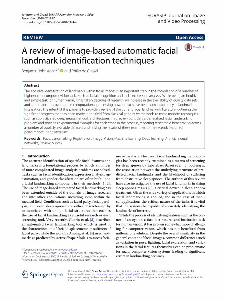
2.2.1 Measuring performancePerformance metrics will vary depending upon the objec-tive definition; Devries et al. [2] used expression classifica-tion accuracy while Tabatabaei Balaei et al. [5] measuredperformance based on rates of correct OSA diagnosis.While these measures determine overall system perfor-mance, measuring facial landmarking accuracy is requiredto ensure landmark predictions are acceptable. This iscompleted by comparing the predictions made by the sys-tem to a set of ‘ground truth’ landmarks which have beenmanually annotated by one or more human experts (seeFigs. 1 and 2).
Johnston and Chazal EURASIP Journal on Image and Video Processing (2018) 2018:86 Page 3 of 23
Fig. 1 Example annotated image. Example training image providedfor the second facial landmark localisation competition held inconjunction with International Conference on Computer Vision andPattern Recognition (CVPR) 2017 [57]
The simplest comparison is a root mean squared error(RMSE) assessment; where the average distance betweeneach of the N predicted landmarks (xpi , y
pi ) and the corre-
sponding ‘ground truth’ (xti , yti) is calculated on a per land-mark basis. Landmarks that are poorly predicted will bepositioned far their corresponding ground truth locationsand thus contribute to increasing the RMSE value. Oftenthe root mean squared error is normalised by the distancebetween two specific ‘ground truth’ points (NMRSE) suchas the left (xtle, y
tle) and the right (xtre, ytre) outer corners of
the eyes dnorm (see Eq. 2) [10] to allow a fair comparisonbetween faces of different sizes
RMSE = 1N
N∑
i=1
√(xpi − xti
)2 + (ypi − yti
)2, (1)
NRMSE = 1N
N∑
i=1
√(xpi − xti
)2 + (ypi − yti
)2
dnorm, (2)
dnorm =√(
xtle − xtre)2 + (
ytle − ytre)2 (3)
When comparing the performance of different land-marking algorithms against the same dataset, the averageRMSE or NRMSE value over the number of samples inthe dataset (K) may simply be reported. A more detailedsummary of themodel performance can be provided usingthe cumulative error distribution (CED), which plots thecumulative NRMSE against the proportion of images with
an NRMSE of less than or equal to a particular value (e.g.Figs. 11, 12, 13, 14, 15, 16, 17, and 18).A less frequently reported metric is the landmark detec-
tion rate, i.e. the proportion of the N landmarks from theK images, correctly identified by the system. A landmarkis correctly identified if its position is less than a definedEuclidean distance from the ‘ground truth’. Similarly to themean squared error calculations, landmark detection ratecan also occur on a per-image, per-landmark, and overallaverage basis.
Throughout this review paper we will use normalisedroot mean squared error (NRMSE), providingpoint-to-point CED plots to compare the performanceof different landmarking methodologies.
2.3 Stage 2: dataset selectionA correct and appropriate selection of a dataset is cru-cial for the development of any predictive algorithm. Theselected dataset must contain features with sufficient pre-dictive power that the training process can ‘learn’ therelationships within the data. For many problems, such asthe prediction of obstructive sleep apnoea [5] a customdataset is required which itself may be subject to iterationsof improvement to ensure the most appropriate featuresare being used.For many facial analysis problems, there exists large,
publicly available databases with rich feature sets (seeTable 1). The datasets can be divided into two cate-gories: those produced within a controlled environmentand those produced in an uncontrolled environment. Thedevelopment of social networks such as Facebook andFlickr, image search engines such as Google Images andthe ability to obtain images at mass from these sites hasenabled the construction of large datasets of facial imagesin various, uncontrolled situations. These ‘in-the-wild’datasets have proven vital for facial landmarking/analysisproblems where it is important to achieve high levels ofaccuracy without the burden of maintaining a controlledenvironment.While many datasets are available for use, it can be
seen in Table 1 that there is little consistency amongstthe different sets. They have different numbers of sam-ples, image resolutions, and configurations of groundtruth landmarks. Some sets have multiple subjects insome images, while others have multiple images for somesubjects. Many in-the-wild datasets are built from weblinks which may not still be valid. While such datavariety is useful, it can lead to difficulties in compar-ing the performance of facial landmarking algorithms.Unlike image classification problems which often stateperformance using standard reference datasets such asMNIST and CIFAR, facial landmarking literature hasnot benefited from a common means of comparison.
Johnston and Chazal EURASIP Journal on Image and Video Processing (2018) 2018:86 Page 4 of 23
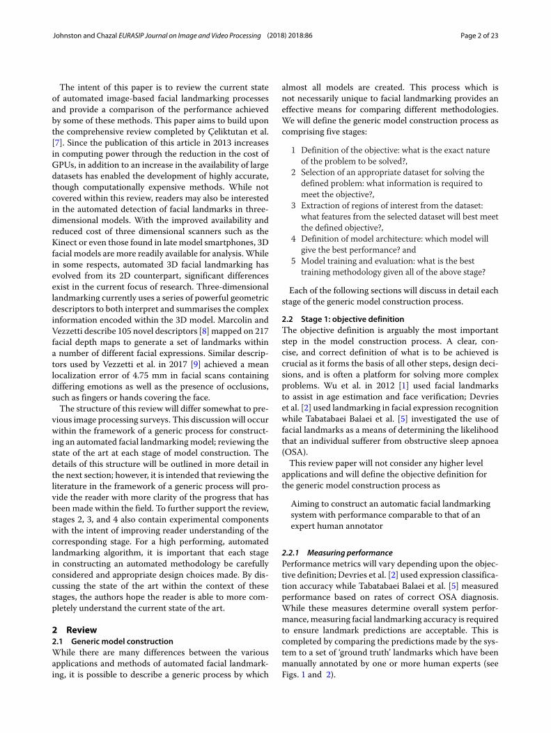
Fig. 2 Examples from public face datasets. These images demonstrate the variety of image types and landmark configurations available withinpublic face datasets. aMULTI-PIE [75], bMUCT [76], c XM2VTS [77], dMenpo (Profile ) [78], e AFLW [79], f PUT [80], g Caltech 10K [81], h BioIDprovided by BioID AG. ©2001 [82], and i HELEN [83]
This problem was identified by Sagonas et al. dur-ing the design of the 300W faces in-the-wild challenge[11]; recognising the variation in annotation schemesbetween public datasets, Sagonas and colleagues pro-posed a semi-automatic landmarking tool [12] to pro-vide a single annotation schema (MULTI-PIE/IBUG 68pt)for a number of datasets. This work provided thefield with a means of comparing different landmark-ing methodologies, while utilising the existing datasets.Subsquent to the second faces in-the-wild challenge[10], the 300W dataset has been used for performancecomparison outside of the context of the landmarkingcompetition [13].
This study reviews and compares the current state of theart in facial landmarking methodologies. To enable thiscomparison, we require datasets which contain the samelandmarking configuration.
The MULTI-PIE landmark configuration as illustratedin Fig. 3 will be used. This configuration is presentwithin many of the datasets contained within Table 1,including the Menpo and 300W datasets.
2.3.1 Ground truth reliabilityWith the exception of the annotations provided byIBUG through their semi-automated annotation tool, face
Johnston and Chazal EURASIP Journal on Image and Video Processing (2018) 2018:86 Page 5 of 23
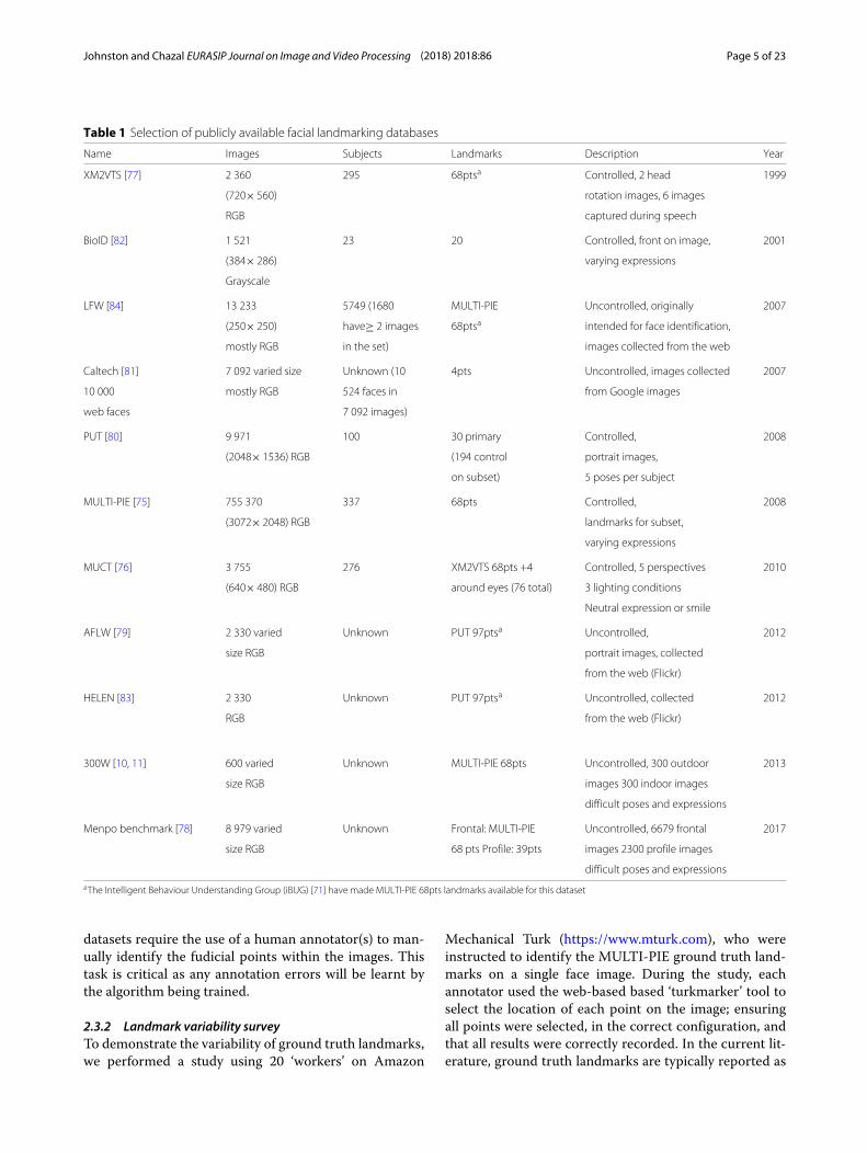
Table 1 Selection of publicly available facial landmarking databases
Name Images Subjects Landmarks Description Year
XM2VTS [77] 2 360 295 68ptsa Controlled, 2 head 1999
(720× 560) rotation images, 6 images
RGB captured during speech
BioID [82] 1 521 23 20 Controlled, front on image, 2001
(384× 286) varying expressions
Grayscale
LFW [84] 13 233 5749 (1680 MULTI-PIE Uncontrolled, originally 2007
(250× 250) have≥ 2 images 68ptsa intended for face identification,
mostly RGB in the set) images collected from the web
Caltech [81] 7 092 varied size Unknown (10 4pts Uncontrolled, images collected 2007
10 000 mostly RGB 524 faces in from Google images
web faces 7 092 images)
PUT [80] 9 971 100 30 primary Controlled, 2008
(2048× 1536) RGB (194 control portrait images,
on subset) 5 poses per subject
MULTI-PIE [75] 755 370 337 68pts Controlled, 2008
(3072× 2048) RGB landmarks for subset,
varying expressions
MUCT [76] 3 755 276 XM2VTS 68pts +4 Controlled, 5 perspectives 2010
(640× 480) RGB around eyes (76 total) 3 lighting conditions
Neutral expression or smile
AFLW [79] 2 330 varied Unknown PUT 97ptsa Uncontrolled, 2012
size RGB portrait images, collected
from the web (Flickr)
HELEN [83] 2 330 Unknown PUT 97ptsa Uncontrolled, collected 2012
RGB from the web (Flickr)
300W [10, 11] 600 varied Unknown MULTI-PIE 68pts Uncontrolled, 300 outdoor 2013
size RGB images 300 indoor images
difficult poses and expressions
Menpo benchmark [78] 8 979 varied Unknown Frontal: MULTI-PIE Uncontrolled, 6679 frontal 2017
size RGB 68 pts Profile: 39pts images 2300 profile images
difficult poses and expressions
aThe Intelligent Behaviour Understanding Group (iBUG) [71] have made MULTI-PIE 68pts landmarks available for this dataset
datasets require the use of a human annotator(s) to man-ually identify the fudicial points within the images. Thistask is critical as any annotation errors will be learnt bythe algorithm being trained.
2.3.2 Landmark variability surveyTo demonstrate the variability of ground truth landmarks,we performed a study using 20 ‘workers’ on Amazon
Mechanical Turk (https://www.mturk.com), who wereinstructed to identify the MULTI-PIE ground truth land-marks on a single face image. During the study, eachannotator used the web-based based ‘turkmarker’ tool toselect the location of each point on the image; ensuringall points were selected, in the correct configuration, andthat all results were correctly recorded. In the current lit-erature, ground truth landmarks are typically reported as
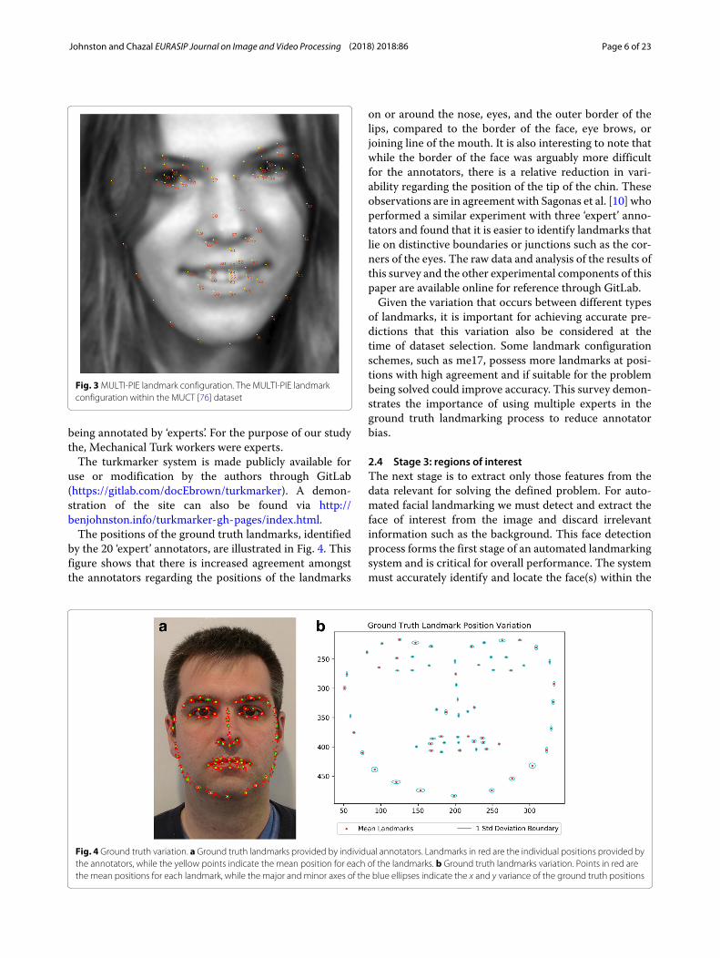
Johnston and Chazal EURASIP Journal on Image and Video Processing (2018) 2018:86 Page 6 of 23
Fig. 3MULTI-PIE landmark configuration. The MULTI-PIE landmarkconfiguration within the MUCT [76] dataset
being annotated by ‘experts’. For the purpose of our studythe, Mechanical Turk workers were experts.The turkmarker system is made publicly available for
use or modification by the authors through GitLab(https://gitlab.com/docEbrown/turkmarker). A demon-stration of the site can also be found via http://benjohnston.info/turkmarker-gh-pages/index.html.The positions of the ground truth landmarks, identified
by the 20 ‘expert’ annotators, are illustrated in Fig. 4. Thisfigure shows that there is increased agreement amongstthe annotators regarding the positions of the landmarks
on or around the nose, eyes, and the outer border of thelips, compared to the border of the face, eye brows, orjoining line of the mouth. It is also interesting to note thatwhile the border of the face was arguably more difficultfor the annotators, there is a relative reduction in vari-ability regarding the position of the tip of the chin. Theseobservations are in agreement with Sagonas et al. [10] whoperformed a similar experiment with three ‘expert’ anno-tators and found that it is easier to identify landmarks thatlie on distinctive boundaries or junctions such as the cor-ners of the eyes. The raw data and analysis of the results ofthis survey and the other experimental components of thispaper are available online for reference through GitLab.Given the variation that occurs between different types
of landmarks, it is important for achieving accurate pre-dictions that this variation also be considered at thetime of dataset selection. Some landmark configurationschemes, such as me17, possess more landmarks at posi-tions with high agreement and if suitable for the problembeing solved could improve accuracy. This survey demon-strates the importance of using multiple experts in theground truth landmarking process to reduce annotatorbias.
2.4 Stage 3: regions of interestThe next stage is to extract only those features from thedata relevant for solving the defined problem. For auto-mated facial landmarking we must detect and extract theface of interest from the image and discard irrelevantinformation such as the background. This face detectionprocess forms the first stage of an automated landmarkingsystem and is critical for overall performance. The systemmust accurately identify and locate the face(s) within the
Fig. 4 Ground truth variation. a Ground truth landmarks provided by individual annotators. Landmarks in red are the individual positions provided bythe annotators, while the yellow points indicate the mean position for each of the landmarks. b Ground truth landmarks variation. Points in red arethe mean positions for each landmark, while the major and minor axes of the blue ellipses indicate the x and y variance of the ground truth positions
Johnston and Chazal EURASIP Journal on Image and Video Processing (2018) 2018:86 Page 7 of 23
image, given variations in lighting, pose, expression, andface appearance. All images must first pass through a facedetector to extract only the important region(s) of interest(ROI) from the data.As this article focuses on facial landmarking techniques,
we only provide a brief overview of face detectors.For the purpose of this article:
We will define the region of interest to be extractedfrom each image to be a single human face.
Two foundational methods of face detection, whichare used as benchmark methods are the Viola-Jones [14]and Histogram of Gradients (HOG) [15] methods. Thesemethods while not currently state of the art achievereasonable accuracy, processing speed, and are in many‘off-the-shelf ’ implementations such as in OpenCV [16]and Dlib.The Viola-Jones method uses a combination of two
main techniques: the representation of Haar-like featuresthrough construction of an ‘integral image’ and a seriesof ‘weak’ classifiers boosted using the Adaboost learningalgorithm. At the very last stage of the cascading classifieris a high-performing perceptron and a decision thresh-old. Using the boosted classifiers and the perceptron layerViola-Jones were able to produce a high performing sys-tem. While generally not used in more modern applica-tions, Viola-Jones face detection still holds its place inliterature as an effective reference method.Dalal and Triggs [15] proposed the HOG method
which produced near-perfect pedestrian detection rateson the MIT pedestrian database. This method convertsthe image into a series of histograms based on the orien-tation and magnitude of pixel gradients within the image.An SVM classifier is then used to identify the face withinthe image based on the values of the histogram. Thisunique pixel gradient signature has proven to be usefulin detecting faces in other image sources such as Li et al.[17] who used camera depth information, as well as clas-sifying if eyes are opened or closed within an image [18].While HOG may no longer be considered state of the art,the method is still demonstrating its relevance and flexi-bility through its direct application in hardware. Suleimanand Sze in 2016 [19] were able to acheive object detectionwithin 1080HD video at 60 frames per second while onlyconsuming 45.3 mW of power. Suleiman and Sze proposethe use of their hardware in embedded, real-time sys-tems which need to minimise power usage. This hardwarebased HOG system has a significant power consumptionadvantage over more modern object detection methodsthat require the use of a dedicated GPU; as an example, themore recent Nvidia GTX 1080TI GPU consumes 250Wof power and recommends a 600 W system power supply,essentially eliminating their use in embedded systems.
First investigated in the early 1990s [20], the use ofconvolutional neural networks (CNN) in face detectionhas recently been the focus of much research effort.In 2007, Osadchy et al. [21] demonstrated the perfor-mance benefit that can be obtained through the use ofCNNs and multi-task learning. Their method trained aCNN (with a similar architecture to the LeNet5 [22])to map images of faces into a low-dimensional manifoldspace, parameterised by the pose of the face. In Osad-chy’s opinion, solving the problem of identifying the faceand determining pose are quite related, so that when thetwo tasks are trained together, an improved performancewould be achieved when compared to using separatenetworks.Theuse of a cascade of CNNswas proposed byHaoxiang
et al. in 2015 [23] and demonstrated an improvement onthe state-of-the-art performance against the Face Detec-tion Data Set and Benchmark (FDDB) [24]. Their methodconsists of a cascading series of three CNN stages. Eachstage is used to detect faces at different resolutions, givenpotential location windows for a face from the previousstage; where the potential detection window for the firststage is defined as the entire image. Each of the three cas-cading stages are themselves composed of two separateCNNs, one designed to detect faces within the potentialdetection window at the given resolution and the fol-lowing designed to calibrate the bounding boxes of thedetected faces to ensure the optimal bounding box for aface is passed onto the next stage.More recently, an implementation of region-based con-
volutional neural networks (R-CNNs) claimed to achievethe best performance to date on FDDB amongst pub-lished results [25]. Region-based CNNs by Girshick et al.in 2014 [26, 27] apply a CNN to warped ‘category indepen-dent’ regions of an image previously computed by a firststage region proposer such as selective search [28]. Themethod by Sun and colleagues pre-trained a model usingthe WIDER-FACE database [24] with hard-negative rein-forcement and a feature concatenation stage [29]. Featureconcatenation combines the features of selected convolu-tional layers before they are passed onto the subsequentlayers in the network. These extracted features providegreater granularity of the through the combination ofhigh- and low-level convolutional layers.Other recent studies have investigated the use of CNNs
in conjunction with other classification techniques: Zhanet al. in 2015 [30] and Tao et al. in 2016 [31] usedCNNs in combination with AdaBoost and SVMs, whileWang et al. in 2016 [32] used a multi-task learningapproach combining classification of the presence orabsence of a face in addition to the coordinates of the facialbounding box.For further details on face dection the authors recom-
mend [33, 34].
Johnston and Chazal EURASIP Journal on Image and Video Processing (2018) 2018:86 Page 8 of 23
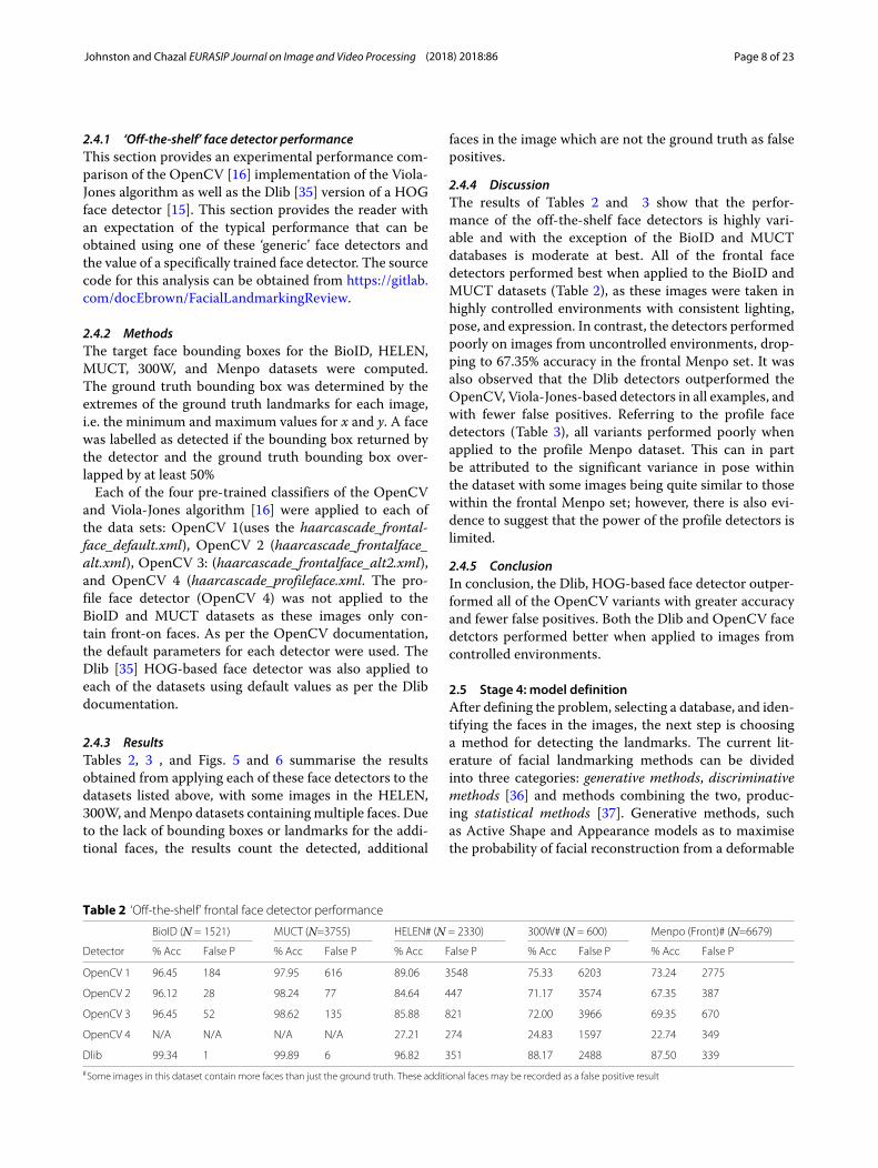
2.4.1 ‘Off-the-shelf’ face detector performanceThis section provides an experimental performance com-parison of the OpenCV [16] implementation of the Viola-Jones algorithm as well as the Dlib [35] version of a HOGface detector [15]. This section provides the reader withan expectation of the typical performance that can beobtained using one of these ‘generic’ face detectors andthe value of a specifically trained face detector. The sourcecode for this analysis can be obtained from https://gitlab.com/docEbrown/FacialLandmarkingReview.
2.4.2 MethodsThe target face bounding boxes for the BioID, HELEN,MUCT, 300W, and Menpo datasets were computed.The ground truth bounding box was determined by theextremes of the ground truth landmarks for each image,i.e. the minimum and maximum values for x and y. A facewas labelled as detected if the bounding box returned bythe detector and the ground truth bounding box over-lapped by at least 50%Each of the four pre-trained classifiers of the OpenCV
and Viola-Jones algorithm [16] were applied to each ofthe data sets: OpenCV 1(uses the haarcascade_frontal-face_default.xml), OpenCV 2 (haarcascade_frontalface_alt.xml), OpenCV 3: (haarcascade_frontalface_alt2.xml),and OpenCV 4 (haarcascade_profileface.xml. The pro-file face detector (OpenCV 4) was not applied to theBioID and MUCT datasets as these images only con-tain front-on faces. As per the OpenCV documentation,the default parameters for each detector were used. TheDlib [35] HOG-based face detector was also applied toeach of the datasets using default values as per the Dlibdocumentation.
2.4.3 ResultsTables 2, 3 , and Figs. 5 and 6 summarise the resultsobtained from applying each of these face detectors to thedatasets listed above, with some images in the HELEN,300W, andMenpo datasets containing multiple faces. Dueto the lack of bounding boxes or landmarks for the addi-tional faces, the results count the detected, additional
faces in the image which are not the ground truth as falsepositives.
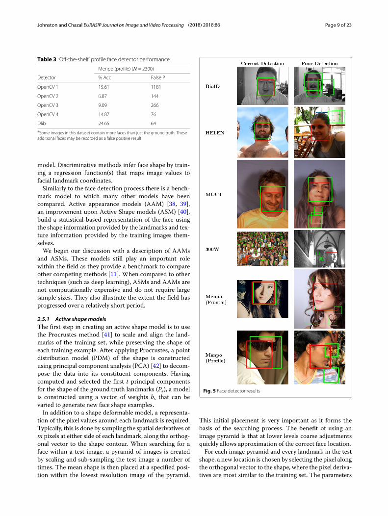
2.4.4 DiscussionThe results of Tables 2 and 3 show that the perfor-mance of the off-the-shelf face detectors is highly vari-able and with the exception of the BioID and MUCTdatabases is moderate at best. All of the frontal facedetectors performed best when applied to the BioID andMUCT datasets (Table 2), as these images were taken inhighly controlled environments with consistent lighting,pose, and expression. In contrast, the detectors performedpoorly on images from uncontrolled environments, drop-ping to 67.35% accuracy in the frontal Menpo set. It wasalso observed that the Dlib detectors outperformed theOpenCV, Viola-Jones-based detectors in all examples, andwith fewer false positives. Referring to the profile facedetectors (Table 3), all variants performed poorly whenapplied to the profile Menpo dataset. This can in partbe attributed to the significant variance in pose withinthe dataset with some images being quite similar to thosewithin the frontal Menpo set; however, there is also evi-dence to suggest that the power of the profile detectors islimited.
2.4.5 ConclusionIn conclusion, the Dlib, HOG-based face detector outper-formed all of the OpenCV variants with greater accuracyand fewer false positives. Both the Dlib and OpenCV facedetctors performed better when applied to images fromcontrolled environments.
2.5 Stage 4: model definitionAfter defining the problem, selecting a database, and iden-tifying the faces in the images, the next step is choosinga method for detecting the landmarks. The current lit-erature of facial landmarking methods can be dividedinto three categories: generative methods, discriminativemethods [36] and methods combining the two, produc-ing statistical methods [37]. Generative methods, suchas Active Shape and Appearance models as to maximisethe probability of facial reconstruction from a deformable
Table 2 ‘Off-the-shelf’ frontal face detector performance
BioID (N = 1521) MUCT (N=3755) HELEN# (N = 2330) 300W# (N = 600) Menpo (Front)# (N=6679)Detector % Acc False P % Acc False P % Acc False P % Acc False P % Acc False P
OpenCV 1 96.45 184 97.95 616 89.06 3548 75.33 6203 73.24 2775
OpenCV 2 96.12 28 98.24 77 84.64 447 71.17 3574 67.35 387
OpenCV 3 96.45 52 98.62 135 85.88 821 72.00 3966 69.35 670
OpenCV 4 N/A N/A N/A N/A 27.21 274 24.83 1597 22.74 349
Dlib 99.34 1 99.89 6 96.82 351 88.17 2488 87.50 339
#Some images in this dataset contain more faces than just the ground truth. These additional faces may be recorded as a false positive result
Johnston and Chazal EURASIP Journal on Image and Video Processing (2018) 2018:86 Page 9 of 23
Table 3 ‘Off-the-shelf’ profile face detector performance
Menpo (profile) (N = 2300)
Detector % Acc False P
OpenCV 1 15.61 1181
OpenCV 2 6.87 144
OpenCV 3 9.09 266
OpenCV 4 14.87 76
Dlib 24.65 64
#Some images in this dataset contain more faces than just the ground truth. Theseadditional faces may be recorded as a false positive result
model. Discriminative methods infer face shape by train-ing a regression function(s) that maps image values tofacial landmark coordinates.Similarly to the face detection process there is a bench-
mark model to which many other models have beencompared. Active appearance models (AAM) [38, 39],an improvement upon Active Shape models (ASM) [40],build a statistical-based representation of the face usingthe shape information provided by the landmarks and tex-ture information provided by the training images them-selves.We begin our discussion with a description of AAMs
and ASMs. These models still play an important rolewithin the field as they provide a benchmark to compareother competing methods [11]. When compared to othertechniques (such as deep learning), ASMs and AAMs arenot computationally expensive and do not require largesample sizes. They also illustrate the extent the field hasprogressed over a relatively short period.
2.5.1 Active shapemodelsThe first step in creating an active shape model is to usethe Procrustes method [41] to scale and align the land-marks of the training set, while preserving the shape ofeach training example. After applying Procrustes, a pointdistribution model (PDM) of the shape is constructedusing principal component analysis (PCA) [42] to decom-pose the data into its constituent components. Havingcomputed and selected the first t principal componentsfor the shape of the ground truth landmarks (Ps), a modelis constructed using a vector of weights bs that can bevaried to generate new face shape examples.In addition to a shape deformable model, a representa-
tion of the pixel values around each landmark is required.Typically, this is done by sampling the spatial derivatives ofm pixels at either side of each landmark, along the orthog-onal vector to the shape contour. When searching for aface within a test image, a pyramid of images is createdby scaling and sub-sampling the test image a number oftimes. The mean shape is then placed at a specified posi-tion within the lowest resolution image of the pyramid.
Fig. 5 Face detector results
This initial placement is very important as it forms thebasis of the searching process. The benefit of using animage pyramid is that at lower levels coarse adjustmentsquickly allows approximation of the correct face location.For each image pyramid and every landmark in the test
shape, a new location is chosen by selecting the pixel alongthe orthogonal vector to the shape, where the pixel deriva-tives are most similar to the training set. The parameters
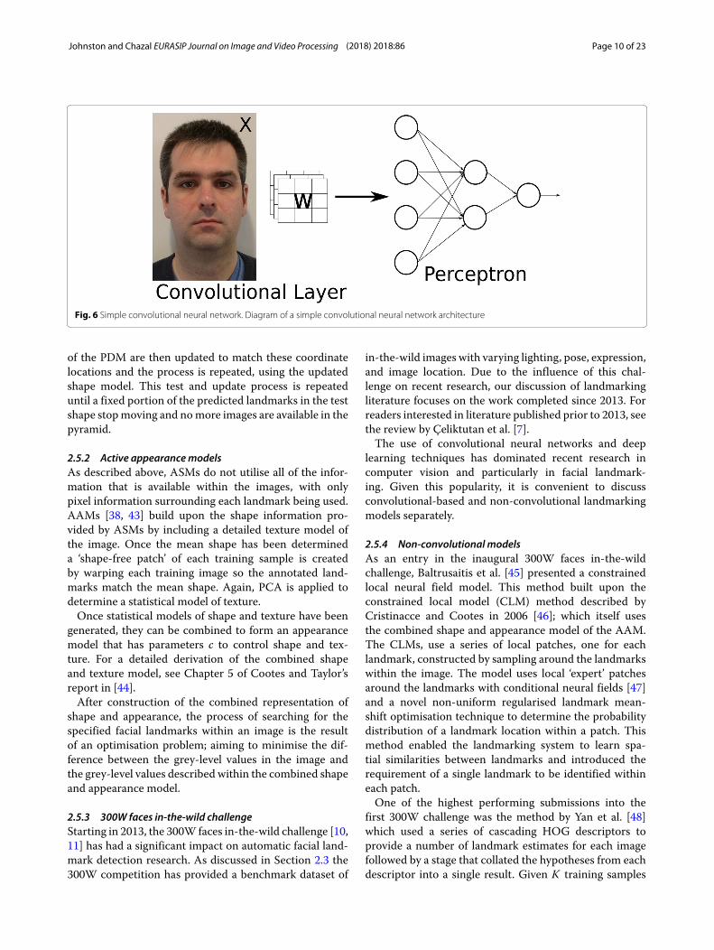
Johnston and Chazal EURASIP Journal on Image and Video Processing (2018) 2018:86 Page 10 of 23
Fig. 6 Simple convolutional neural network. Diagram of a simple convolutional neural network architecture
of the PDM are then updated to match these coordinatelocations and the process is repeated, using the updatedshape model. This test and update process is repeateduntil a fixed portion of the predicted landmarks in the testshape stopmoving and nomore images are available in thepyramid.
2.5.2 Active appearancemodelsAs described above, ASMs do not utilise all of the infor-mation that is available within the images, with onlypixel information surrounding each landmark being used.AAMs [38, 43] build upon the shape information pro-vided by ASMs by including a detailed texture model ofthe image. Once the mean shape has been determineda ‘shape-free patch’ of each training sample is createdby warping each training image so the annotated land-marks match the mean shape. Again, PCA is applied todetermine a statistical model of texture.Once statistical models of shape and texture have been
generated, they can be combined to form an appearancemodel that has parameters c to control shape and tex-ture. For a detailed derivation of the combined shapeand texture model, see Chapter 5 of Cootes and Taylor’sreport in [44].After construction of the combined representation of
shape and appearance, the process of searching for thespecified facial landmarks within an image is the resultof an optimisation problem; aiming to minimise the dif-ference between the grey-level values in the image andthe grey-level values described within the combined shapeand appearance model.
2.5.3 300W faces in-the-wild challengeStarting in 2013, the 300W faces in-the-wild challenge [10,11] has had a significant impact on automatic facial land-mark detection research. As discussed in Section 2.3 the300W competition has provided a benchmark dataset of
in-the-wild images with varying lighting, pose, expression,and image location. Due to the influence of this chal-lenge on recent research, our discussion of landmarkingliterature focuses on the work completed since 2013. Forreaders interested in literature published prior to 2013, seethe review by Çeliktutan et al. [7].The use of convolutional neural networks and deep
learning techniques has dominated recent research incomputer vision and particularly in facial landmark-ing. Given this popularity, it is convenient to discussconvolutional-based and non-convolutional landmarkingmodels separately.
2.5.4 Non-convolutional modelsAs an entry in the inaugural 300W faces in-the-wildchallenge, Baltrusaitis et al. [45] presented a constrainedlocal neural field model. This method built upon theconstrained local model (CLM) method described byCristinacce and Cootes in 2006 [46]; which itself usesthe combined shape and appearance model of the AAM.The CLMs, use a series of local patches, one for eachlandmark, constructed by sampling around the landmarkswithin the image. The model uses local ‘expert’ patchesaround the landmarks with conditional neural fields [47]and a novel non-uniform regularised landmark mean-shift optimisation technique to determine the probabilitydistribution of a landmark location within a patch. Thismethod enabled the landmarking system to learn spa-tial similarities between landmarks and introduced therequirement of a single landmark to be identified withineach patch.One of the highest performing submissions into the
first 300W challenge was the method by Yan et al. [48]which used a series of cascading HOG descriptors toprovide a number of landmark estimates for each imagefollowed by a stage that collated the hypotheses from eachdescriptor into a single result. Given K training samples
Johnston and Chazal EURASIP Journal on Image and Video Processing (2018) 2018:86 Page 11 of 23
{Ik,X∗
k,X0k; k = 1 . . .K
}where Ik is the image/texture
information, X∗k are the ground truth landmarks, and X0
k,the initialised landmarks [48] (the mean face shape at thestart of the process). The objective is to learn a regressionfunction f minimising the mean squared error betweenthe predicted and ground truth landmarks (Eq. 4). Thiscascading model learns complex non-linear relationshipswithin the dataset by dividing f into a series of T sim-pler regression functions (f0, f1, f1 . . . fT ) and using theHadamard product represented by ◦ (Eq. 5). The outputof each sub-function is passed as the input to the follow-ing stage and a linear transformationWt is applied (Eq. 6)to a feature transform
(�
(Xk
t−1, Ik))
thus encoding theimage information around the shape.
f = argminf
K∑
k=1
∥∥f(X0k, Ik
) − X∗k∥∥2 (4)
f = f0 ◦ f1 ◦ f2 ◦ · · · ◦ fT (5)
Where
Xtk = ft
(Xt−1k , Ik
) = Wt · �(Xt−1k , Ik
)(6)
The authors noted that their method is highly sensitiveto shape initialisation and that the accepted benchmarkfor face detection of a 50% bounding box overlap wasinsufficient. To reduce the influence of initialisation, thebounding boxes determined by the face detector are ran-domly scaled and shifted, generating multiple hypothesesof landmark positions for each image. Given that multi-ple sets of landmarks are estimated for each image, Yan etal. propose two methods for combining these results. Thefirst method: learn to rank, assumes that for each image atleast one hypothesis is better than the others and definesa function that ranks and selects the best one from theset. The second method learn to combine assumes that foran image the information contained within the entire setof hypotheses is complementary to the final solution andthus defines a function that combines the hypotheses intoa single result. The parameters of both of these functionscan be determined by solving with a structural SVM.
2.5.5 Cascade shape regressionmodelsCompared with their generative counterparts, discrimi-native landmarking methods have demonstrated superiorperformance in uncontrolled conditions [36]. This per-formance has been further improved through the devel-opment of a cascade of linear regression models that arecapable of describing complex non-linear relationships.Asthana et al. [36] outline such a method which hasresemblance to AAMs models, defining a shape model as
x(p) = sR (x̄ + �sg) + t; i = 1 . . .N (7)
Where x ∈ �2N×1 is a vector form of X ∈ �N×2, s is thescale,R is the rotationmatri, and t is a translational vector.The vector �sg specifies non-rigid shape variation; thus,p = [
s; rx; ry; rz; tx; ty; g]T . By specifying a set of shape
parameters P∗ = {p∗i}Kk=0 that are defined by the ground
truth shape. Asthana et al. define their objective as learn-ing a function from an initial estimate of pwhich producesthe ground truth p∗. The function that converts the initialshape estimate is a sequence of regression functions [49].For each of the K training shapes, the parameters definingthe shape model are randomly sampled within a definedrange around the ground truth parameters P∗ producinga set of J perturbed shape parameters
{p(1)j
}Jj=1
. A linearrelationship between the input image I and the perturbedparameters p(1)
j is described as
p∗ = p(1) + f(I, x
(p(1)
))W + b (8)
where the function f could return SIFT [50] or HOGfeatures around each landmark matrix. The linear rela-tionship described by Eq. 8 is unable to map the perturbedshape parameters p(1) to the ground truth p∗. Thus, a cas-cading series of regression functions is trained by findingW̃ =[W ; b] to solve the following problem:
arg minW(1),b(1)
K∑
k=1
J∑
j=1
∥∥∥�p(1)kj − f̃
(Ii, p(1)
kj
)W̃(1)
∥∥∥2
(9)
Where f̃(I,p) =[ f (I,p) 1] and�p(1)kj = p∗
k − p(1)kj and j
is the index of perturbation. By repeatedly solving for W̃(1)
and updating pkj, the perturbed parameters approach theground truth. In their work, Asthana et al. propose a par-allel method of cascade linear regression that does notrely on the perturbations of previous iterations and ben-efits from executing the process in parallel. This parallelcascade of linear regression uses only the statistics of theprevious level, removing the need to propagate through allof the samples and iterations. One further benefit of thismethod is that if additional training data is made available,the costly process of retraining through all combinationsof iterations and perturbations is not required as thecascade of regression functions are trained individually.Deng et al. in 2015 [37] extended the cascade
shape model, describing a multi-view, multi-scale, andmulti-component cascade shape model (M3CSR). Deng’smethod first applied a six-component deformable partmodel face detector to divide the training samples intofront, left, and right profile views. By grouping the images,the variation within each view set is reduced, improvingthe model’s performance with an increased range in pose.
Johnston and Chazal EURASIP Journal on Image and Video Processing (2018) 2018:86 Page 12 of 23
After finding the HOG descriptors for each of theimages in each set, the cascade shape regression process isexecuted in a coarse to fine manner; starting with a smallinstance of the face and then doubling the face’s size toproduce a second scaled image. This coarse to fine pro-cess improves the speed and accuracy of convergence byallowing for gross changes to landmark position at thecoarse level and precision adjustment within the higherresolution image.The final aspect of the M3CSR process is the multi-
component stage to compensate for differences inlandmark stability, similar to that described in theSection 2.3.2. Given differences in facial expression or nat-ural variation in the location of particular landmarks suchas the tip of the nose compared to the cheek, an additionalalignment process was executed for each landmark:
argminWt
K∑
k=1
∥∥∥(X∗k − Xt−1
k
)− Wt�
(Ik,Xt−1
k
)∥∥∥2
2(10)
where t is the iteration number, X0k is the initialised shape
coordinates, Wt is the linear transform matrix, and �
represents the shape index feature descriptor, correspond-ing to either the front, left, or right profile views. Notethe similarities between Eqs. 9 and 10 which follows thesimilar processes used by Deng et al. and Asthana etal.; applying the variation within the landmarks them-selves, instead of intentional perturbations to construct analigned shape model.Having separated the training images on the basis of
pose and doubled the scale of the images, the training pro-cess comprises of iterating through each set of poses andscales: generating 10 different shape initialisations, com-puting the HOG features around each landmark, findingW, and updating the shape Xt
k = Xt−1k +Wt�
(Xt−1k , Ik
).
During their experimentation, Deng and colleagues alsoconfirmed the performance increase of M3CSR whencompared with M1CSR (multi-view cascade shape regres-sion) and M2CSR (multi-view, multi-scale cascade shaperegression) models.
2.5.6 Convolutional neural network landmarkingmodelsThe use of CNNs has gained much popularity recentlywithin the field. This popularity can partly be attributedto the availability of large datasets and high perfor-mance, affordable computational hardware such as graph-ics processing units (GPUs). The use of CNNs have alsoincreased after the significant increase in ImageNet clas-sification performance achieved by Krizhevsky et al. [51]with AlexNet. Many of the current leading classifiers onbenchmark datasets such as MNIST [22, 52], CIFAR-10[53, 54], and CIFAR-100 [53, 55] are based on CNNs. Thishas been particularly evident in computer vision where
CNNs or deep learning has provided effective solutionsfor face detection, facial landmark prediction, and otherproblems.
2.5.7 Convolutional neural networksIn its most basic form, a convolutional neural networkis a simple perceptron (or neural network) with a pre-ceeding stage that performs a convolution operation(Q = I ∗ W + b) on an input image I, given a set ofweights W and biases b [56]. Similarly to the weightswithin the perceptron, backpropagation is applied to opti-miseW,b for the given cost function to adjust the weightsaccording to their contribution to the error. Thus, the con-volutional layers form a set of feature extracters for thesystem. This is one of the most powerful aspects of CNNs;rather than using manually crafted features such as Haar-like or HOG features, the system automatically ‘learns’ theoptimal features for the dataset and the objective of thenetwork. Additionally, CNNs, unlike many other modeldesigns, are able to continue to improve their performanceas data is added to the training set.As outlined in the Section 2.5.4 as well as in [11] and
[10], the first two 300W competitions received submis-sions using a number of different methodologies includingdeep learning. In contrast to the 2017Menpo Facial Land-mark Localisation Challenge [57], all submissions to thecompetition utilised deep learning. Deep learning meth-ods have won every recent facial landmarking challenge:Zhou et al. in 2013 [58], Fan and Zhou in 2015 [59], andYang et al. [60] winning both frontal and profile competi-tions in 2017. The high performance of these techniquesprompted the organisers of the Menpo Challenge to ask“is the current achieved performance good enough?” [61].One of themost common designs of deep learningmod-
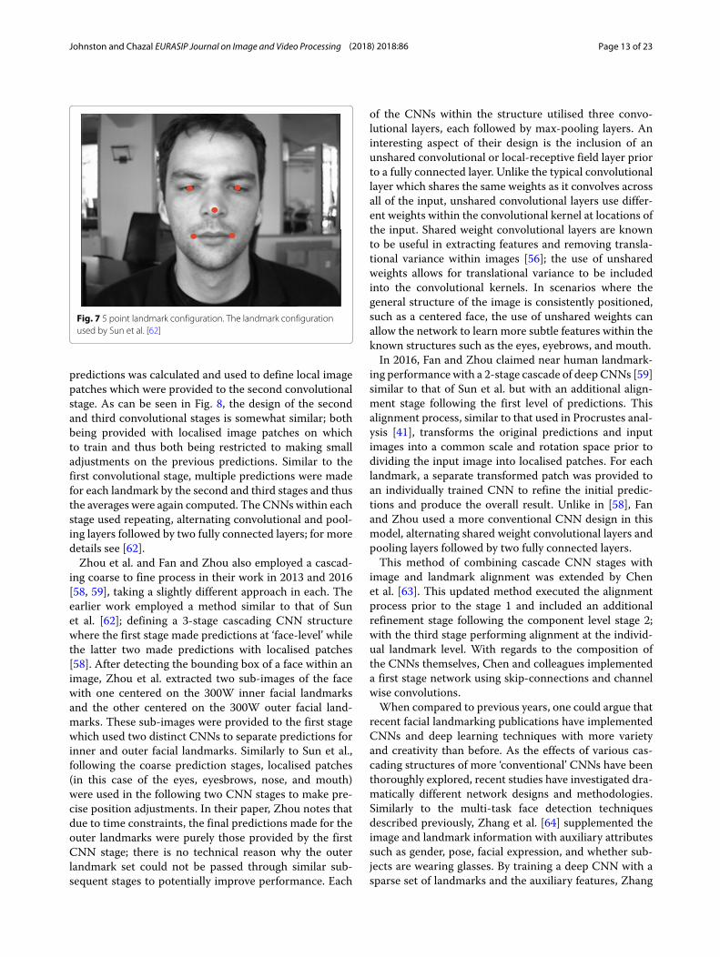
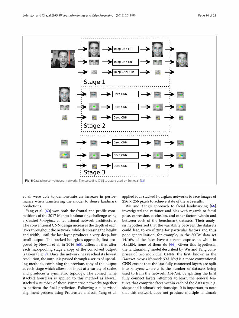
els in facial landmarking is the cascading structure wherea number of different convolutional neural network stagesare connected sequentially to produce the final landmarkpredictions. Typically, cascading networks are employedin a coarse to fine manner, where earlier networks in thecascade make more gross predictions regarding landmarkposition and later stagesmake fine positional adjustments.An early user of this methodology was Sun et al. in 2013[62]. They used three cascading levels to predict fivelandmarks on the face (see Fig. 7). After applying theface detector, Sun et al. constructed three CNNs withinthe first stage: the first CNN received an image of theentire facial region, the second an image of the eyes andnose, and the third of the nose and mouth. The firststage estimated the approximate landmark locations, thuseach network was trained to make coarse predictions ofthe landmark positions within the corresponding regionof the image. The three CNNs observed each landmarkat least twice, and thus multiple predictions for eachlandmark were produced. The average of each of these
Johnston and Chazal EURASIP Journal on Image and Video Processing (2018) 2018:86 Page 13 of 23
Fig. 7 5 point landmark configuration. The landmark configurationused by Sun et al. [62]
predictions was calculated and used to define local imagepatches which were provided to the second convolutionalstage. As can be seen in Fig. 8, the design of the secondand third convolutional stages is somewhat similar; bothbeing provided with localised image patches on whichto train and thus both being restricted to making smalladjustments on the previous predictions. Similar to thefirst convolutional stage, multiple predictions were madefor each landmark by the second and third stages and thusthe averages were again computed. The CNNs within eachstage used repeating, alternating convolutional and pool-ing layers followed by two fully connected layers; for moredetails see [62].Zhou et al. and Fan and Zhou also employed a cascad-
ing coarse to fine process in their work in 2013 and 2016[58, 59], taking a slightly different approach in each. Theearlier work employed a method similar to that of Sunet al. [62]; defining a 3-stage cascading CNN structurewhere the first stage made predictions at ‘face-level’ whilethe latter two made predictions with localised patches[58]. After detecting the bounding box of a face within animage, Zhou et al. extracted two sub-images of the facewith one centered on the 300W inner facial landmarksand the other centered on the 300W outer facial land-marks. These sub-images were provided to the first stagewhich used two distinct CNNs to separate predictions forinner and outer facial landmarks. Similarly to Sun et al.,following the coarse prediction stages, localised patches(in this case of the eyes, eyesbrows, nose, and mouth)were used in the following two CNN stages to make pre-cise position adjustments. In their paper, Zhou notes thatdue to time constraints, the final predictions made for theouter landmarks were purely those provided by the firstCNN stage; there is no technical reason why the outerlandmark set could not be passed through similar sub-sequent stages to potentially improve performance. Each
of the CNNs within the structure utilised three convo-lutional layers, each followed by max-pooling layers. Aninteresting aspect of their design is the inclusion of anunshared convolutional or local-receptive field layer priorto a fully connected layer. Unlike the typical convolutionallayer which shares the same weights as it convolves acrossall of the input, unshared convolutional layers use differ-ent weights within the convolutional kernel at locations ofthe input. Shared weight convolutional layers are knownto be useful in extracting features and removing transla-tional variance within images [56]; the use of unsharedweights allows for translational variance to be includedinto the convolutional kernels. In scenarios where thegeneral structure of the image is consistently positioned,such as a centered face, the use of unshared weights canallow the network to learn more subtle features within theknown structures such as the eyes, eyebrows, and mouth.In 2016, Fan and Zhou claimed near human landmark-
ing performance with a 2-stage cascade of deep CNNs [59]similar to that of Sun et al. but with an additional align-ment stage following the first level of predictions. Thisalignment process, similar to that used in Procrustes anal-ysis [41], transforms the original predictions and inputimages into a common scale and rotation space prior todividing the input image into localised patches. For eachlandmark, a separate transformed patch was provided toan individually trained CNN to refine the initial predic-tions and produce the overall result. Unlike in [58], Fanand Zhou used a more conventional CNN design in thismodel, alternating shared weight convolutional layers andpooling layers followed by two fully connected layers.This method of combining cascade CNN stages with
image and landmark alignment was extended by Chenet al. [63]. This updated method executed the alignmentprocess prior to the stage 1 and included an additionalrefinement stage following the component level stage 2;with the third stage performing alignment at the individ-ual landmark level. With regards to the composition ofthe CNNs themselves, Chen and colleagues implementeda first stage network using skip-connections and channelwise convolutions.When compared to previous years, one could argue that
recent facial landmarking publications have implementedCNNs and deep learning techniques with more varietyand creativity than before. As the effects of various cas-cading structures of more ‘conventional’ CNNs have beenthoroughly explored, recent studies have investigated dra-matically different network designs and methodologies.Similarly to the multi-task face detection techniquesdescribed previously, Zhang et al. [64] supplemented theimage and landmark information with auxiliary attributessuch as gender, pose, facial expression, and whether sub-jects are wearing glasses. By training a deep CNN with asparse set of landmarks and the auxiliary features, Zhang
Johnston and Chazal EURASIP Journal on Image and Video Processing (2018) 2018:86 Page 14 of 23
Fig. 8 Cascading convolutional networks. The cascading CNN structure used by Sun et al. [62]
et al. were able to demonstrate an increase in perfor-mance when transferring the model to dense landmarkpredictions.Yang et al. [60] won both the frontal and profile com-
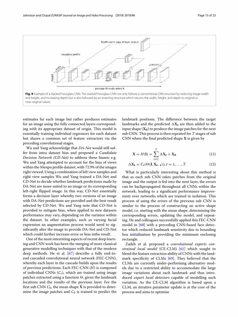
petitions of the 2017 Menpo landmarking challenge usinga stacked hourglass convolutional network architecture.The conventional CNN design increases the depth of eachlayer throughout the network, while decreasing the heightand width, until the last layer produces a very deep, butsmall output. The stacked hourglass approach, first pro-posed by Newall et al. in 2016 [65], differs in that aftereach max-pooling stage a copy of the convolved outputis taken (Fig. 9). Once the network has reached its lowestresolution, the output is passed through a series of upscal-ing methods, combining the previous copy of the outputat each stage which allows for input at a variety of scalesand produces a symmetric topology. The coined namestacked hourglass is applied to this method as Newallstacked a number of these symmetric networks togetherto perform the final prediction. Following a supervisedalignment process using Procrustes analysis, Yang et al.
applied four stacked hourglass networks to face images of256 × 256 pixels to achieve state of the art results.Wu and Yang’s approach to facial landmarking [66]
investigated the variance and bias with regards to facialpose, expression, occlusion, and other factors within andbetween each of the benchmark datasets. Their analy-sis hypothesised that the variability between the datasetscould lead to overfitting for particular factors and thuspoor generalisation, for example, in the 300W data set14.16% of the faces have a scream expression while inHELEN, none of them do [66]. Given this hypothesis,the landmarking model described by Wu and Yang com-prises of two individual CNNs; the first, known as theDataset-Across Network (DA-Net) is a more conventionalCNN except that the last fully connected layers are splitinto n layers where n is the number of datasets beingused to train the network. DA-Net, by splitting the finalfully connect layers, attempts to learn the general fea-tures that comprise faces within each of the datasets, e.g.shape and landmark relationships. It is important to notethat this network does not produce multiple landmark
Johnston and Chazal EURASIP Journal on Image and Video Processing (2018) 2018:86 Page 15 of 23
Fig. 9 Example of a stacked hourglass CNN. The stacked hourglass CNN not only follows a conventional CNN structure by reducing image widthand height, and increasing depth but is also followed by an inverting structure which returns the width, height, and depth to original ornear-original values
estimates for each image but rather produces estimatesfor an image using the fully connected layers correspond-ing with its appropriate dataset of origin. This model isessentially training individual regressors for each datasetbut shares a common set of feature extractors via thepreceding convolutional stages.Wu and Yang acknowledge that DA-Net would still suf-
fer from intra dataset bias and proposed a CandidateDecision Network (CD-Net) to address these biases; e.g.Wu and Yang attempted to account for the bias of viewswithin theMenpo profile dataset, with 72.9% of the imagesright viewed. Using a combination of left view samples andright view samples Wu and Yang trained a DA-Net andCD-Net to decide whether landmark predictions made byDA-Net are more suited to an image or its correspondingleft-right flipped image. In this way, CD-Net essentiallyforms a decision layer whereby two versions of an imagewith DA-Net predictions are provided and the best resultselected by CD-Net. Wu and Yang note that CD-Net isprovided to mitigate bias, when applied to new datasetsperformance may vary, depending on the variance withinthe dataset. In other examples, such as varying facialexpression an augmentation process would need to sig-nificantly alter the image to provide DA-Net and CD-Netwhich could further increase error or bias inthe result.One of themost interesting aspects of recent deep learn-
ing and CNNwork has been the merging of more classicalgenerative modelling techniques with that of the moderndeep methods. He et al. [67] describe a fully end-to-end cascaded convolutional neural network (FEC-CNN),whereby each layer in the cascade builds upon the resultsof previous predictions. Each FEC-CNN (H) is composedof individual CNNs (Ct), which are trained using imagepatches extracted using a function �, given the landmarklocations and the results of the previous layer. For thefirst sub CNN C0, the mean shape X̄ is provided to deter-mine the image patches and C0 is trained to predict the
landmark positions. The difference between the targetlandmarks and the predicted �Xt are then added to theinput shape (X0) to produce the image patches for the nextsub CNN. This process is then repeated for T stages of subCNN where the final predicted shape X is given by
X = H(I) =T∑
t=1�Xt + X0 (11)
�Xt = Ct(�(I,Xt−1)), t = 1, . . . ,T (12)
What is particularly interesting about this method isthat as each sub CNN takes patches from the originalimage and the output is fed into the next layer, the errorscan be backpropagated throughout all CNNs within thenetwork, leading to a significant performance improve-ment over networks which are trained in isolation. Thisprocess of using the errors of the previous sub CNN issimilar to the process of constructing an active shapemodel, i.e. starting with the mean shape, determining thecorresponding errors, updating the model, and repeat-ing. He and colleagues successfully applied this FEC-CNNmodel in [68] with a preceding CNN-based face detec-tor which reduced landmark sensitivity due to boundingbox initialisation by providing the minimum enclosingrectangle.Zadeh et al. proposed a convolutional experts con-
strained local model (CE-CLM) [61] which sought toblend the feature extraction ability of CNNs with the land-mark specificity of CLMs [69]. They believed that theCLMs are currently under-performing alternative mod-els due to a restricted ability to accommodate the largeimage variations about each landmark and thus intro-duced expert local detectors capable of modelling suchvariation. As the CE-CLM algorithm is based upon aCLM, an iterative parameter update is at the core of theprocess and aims to optimise
Johnston and Chazal EURASIP Journal on Image and Video Processing (2018) 2018:86 Page 16 of 23
p∗ = argminp
[ N∑
i=1−Di(xi; I) + �(p)
](13)
where xi ∈ �1×2 is a subset of X ∈ �N×2. Similarly toEq. 8, p∗ are the optimal parameters defining landmarkposition and p denotes the current estimate for the loca-tion of xi. Di(xi; I) is the probability of the ith landmarkbeing in position xi for input image I and �(p) is a reg-ularisation function. One should note that the definitionof p∗ and p are identical to that described within Eq. 7and in contrast to many other methods Eqs. 7 and 13 useground truth and predicted landmarks in vector form xnot the corresponding matrix form X. The most impor-tant part of the CE-CLM design is the ConvolutionalExperts Network (CEN) which takes landmark localisedimage patches and returns the probability map Di(xi; I),which as shown in Eq. 13 is crucial in finding the optimummodel parameters.The CEN is a specially crafted network composed of
three distinct layers: a contrast normalising convolutionallayer, a generic convolutional layer, and a mixture ofexperts (ME) convolutional layer. Upon providing thenetwork with a localised image patch, the contrast nor-malising layer performs Z score normalisation on theimage prior to convolving with a ReLU-based kernel of thegeneric convolution layer. The first two layers of the net-work essentially prepare the data for the third and finalME-layer which produces the final alignment probabili-ties for the image patch. The ME-layer is a convolutionallayer with a kernel using a sigmoid activation functionwhich produces the response map or probabilities of land-mark alignment within an image patch. The responsemaps are then combined with a non-negative weight finallayer which too uses a sigmoid activation function tocompute Di(xi; I). Zadeh et al. noted that a 1 × 1 ker-nel size with no pooling layers was selected to increasethe resolution of the landmark prediction space and thatthe ME-layer had a significant impact on the overall per-formance. Unlike other CNNs, increasing the depth ofthe CEN did not improve the performance of the net-work while changes to the ME-layer such as removing theconstraint of non-negative weights result in a significantreduction in performance.Consistent with CLMs and cascade regression models,
Zadeh et al. used point distribution models (PDMs) tocontrol landmark locations and penalise irregular shapesthrough �(p). Using Eq. 7 and given an initial CE-CLMestimate p, the required updates�p are iteratively appliedin response to the positions provided by CEN to deter-mine the final model that maps the input image to thecorresponding face shape.The final CNN model discussed is the Deep Alignment
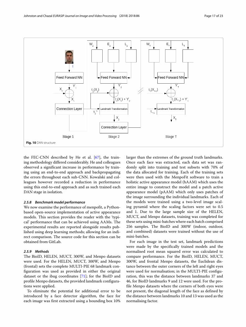
Network (DAN) by Kowalski et al. [70], which was inspiredby the cascade shape regression (CSR) model. Like CSR
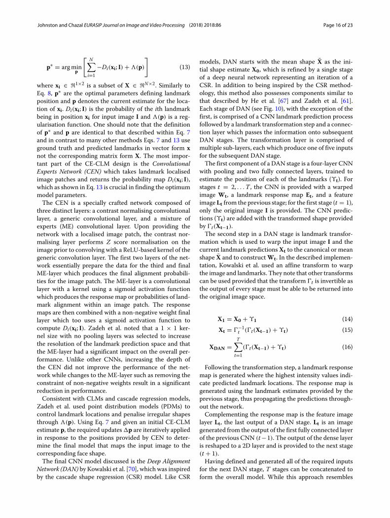
models, DAN starts with the mean shape X̄ as the ini-tial shape estimate X0, which is refined by a single stageof a deep neural network representing an iteration of aCSR. In addition to being inspired by the CSR method-ology, this method also possesses components similar tothat described by He et al. [67] and Zadeh et al. [61].Each stage of DAN (see Fig. 10), with the exception of thefirst, is comprised of a CNN landmark prediction processfollowed by a landmark transformation step and a connec-tion layer which passes the information onto subsequentDAN stages. The transformation layer is comprised ofmultiple sub-layers, each which produce one of five inputsfor the subsequent DAN stage.The first component of a DAN stage is a four-layer CNN
with pooling and two fully connected layers, trained toestimate the position of each of the landmarks (ϒt). Forstages t = 2, . . .T , the CNN is provided with a warpedimage Wt, a landmark response map Et, and a featureimage Lt from the previous stage; for the first stage (t = 1),only the original image I is provided. The CNN predic-tions (ϒt) are added with the transformed shape providedby �t(Xt−1).The second step in a DAN stage is landmark transfor-
mation which is used to warp the input image I and thecurrent landmark predictionsXt to the canonical or meanshape X̄ and to constructWt. In the described implemen-tation, Kowalski et al. used an affine transform to warpthe image and landmarks. They note that other transformscan be used provided that the transform �t is invertible asthe output of every stage must be able to be returned intothe original image space.
X1 = X0 + ϒ1 (14)Xt = �−1
t (�t(Xt−1) + ϒt) (15)
XDAN =T∑
t=1(�t(Xt−1) + ϒt) (16)
Following the transformation step, a landmark responsemap is generated where the highest intensity values indi-cate predicted landmark locations. The response map isgenerated using the landmark estimates provided by theprevious stage, thus propagating the predictions through-out the network.Complementing the response map is the feature image
layer Lt, the last output of a DAN stage. Lt is an imagegenerated from the output of the first fully connected layerof the previous CNN (t−1). The output of the dense layeris reshaped to a 2D layer and is provided to the next stage(t + 1).Having defined and generated all of the required inputs
for the next DAN stage, T stages can be concatenated toform the overall model. While this approach resembles
Johnston and Chazal EURASIP Journal on Image and Video Processing (2018) 2018:86 Page 17 of 23
Fig. 10 DAN structure
the FEC-CNN described by He et al. [67], the train-ing methodology differed considerably. He and colleaguesobserved a significant increase in performance by train-ing using an end-to-end approach and backpropagatingthe errors throughout each sub-CNN. Kowalski and col-leagues however recorded a reduction in performanceusing this end-to-end approach and as such trained eachDAN stage in isolation.
2.5.8 Benchmarkmodel performanceWe now examine the performance of menpofit, a Python-based open-source implementation of active appearancemodels. This section provides the reader with the ‘typi-cal’ performance that can be achieved using AAMs. Theexperimental results are reported alongside results pub-lished using deep learning methods; allowing for an indi-rect comparison. The source code for this section can beobtained from GitLab.
2.5.9 MethodsThe BioID, HELEN, MUCT, 300W, and Menpo datasetswere used. For the HELEN, MUCT, 300W, and Menpo(frontal) sets the complete MULTI-PIE 68 landmark con-figuration was used as provided in either the originaldataset or the ibug coordinates [71]; for the BioID andprofile Menpo datasets, the provided landmark configura-tions were applied.To eliminate the potential for additional error to be
introduced by a face detector algorithm, the face foreach image was first extracted using a bounding box 10%
larger than the extremes of the ground truth landmarks.Once each face was extracted, each data set was ran-domly split into training and test subsets with 70% ofthe data allocated for training. Each of the training setswere then used with the MenpoFit software to train aholistic active appearance model (hAAM) which uses theentire image to construct the model and a patch activeappearance model (pAAM) which only uses patches ofthe image surrounding the individual landmarks. Each ofthe models were trained using a two-level image scal-ing pyramid where the scaling factors were set to 0.5and 1. Due to the large sample size of the HELEN,MUCT, and Menpo datasets, training was completed forthese sets usingmini-batches where each batch comprised256 samples. The BioID and 300W (indoor, outdoor,and combined) datasets were trained without the use ofmini-batches.For each image in the test set, landmark predictions
were made by the specifically trained models and thenormalised root mean squared error was calculated tocompare performance. For the BioID, HELEN, MUCT,300W, and frontal Menpo datasets, the Euclidean dis-tance between the outer corners of the left and right eyeswere used for normalisation; in the MULTI-PIE configu-ration, this was the distance between landmarks 37 and46, for BioID landmarks 9 and 12 were used. For the pro-file Menpo datasets where the corners of both eyes werenot present, the diagonal length of the face as defined bythe distance between landmarks 10 and 13 was used as thenormalising factor.
Johnston and Chazal EURASIP Journal on Image and Video Processing (2018) 2018:86 Page 18 of 23
For all methods and all datasets, cumulative error dis-tribution curves were produced. For the BioID, 300W, andthe Menpo datasets, error curves indicating state of theart performance were overlayed and referenced.All models were trained and tested using the high
performance computing facilities provided by the Syd-ney Informatics Hub at the University of Sydney whichinclude Dell PowerEdge R630 and C6320 Server nodes.Each PowerEdge R630 node possess 24Haswell Intel XeonE5-2680 V3 cores with 128 GB of DDR3 RAM, while theC6320 nodes possess 32 Broadwell Intel Xeon E5-2697A-V4 cores also with 128 GB of DDR3 RAM. The resourceutilisation of each model was recorded and is provided inthe Section 2.5.10.
2.5.10 ResultsFigures 11, 12, 13, 14, 15, 16, 17, and 18 describe theperformance of each method on each dataset using cumu-lative error distribution curves, while Table 4 indicates theresources required to produce and test each model. Notethat CPU utilisation is recorded as the average number ofCPUs used over the course of executing the script.
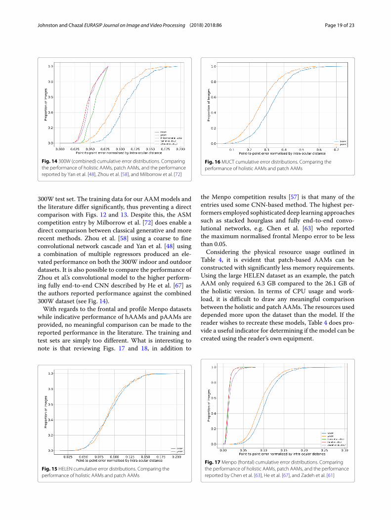
2.5.11 DiscussionObserving the AAM curves across the figures, it can beseen that patch-based AAMs outperform holistic modelsfor almost all datasets; with near-identical performanceusing HELEN (see Fig. 15). This is particularly evidentin the profile Menpo results (Fig. 18) with the holisticmethod essentially unable to model the data. As notedby [66] and [61], the profile Menpo dataset is particu-larly challenging due to the variety of facial poses (somecould plausibly be in the frontal dataset) and an imbal-ance of left/right side facing profile images. The failure ofthe holistic model can be attributed to this variance andthe inability of the model to represent it. Conversely, the
Fig. 11 BioID cumulative error distributions. Comparing theperformance of holistic AAMs, patch AAMs, and the performancereported by Cristinacce and Cootes [46]
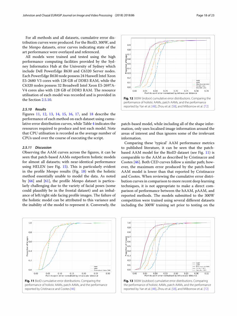
Fig. 12 300W (indoor) cumulative error distributions. Comparing theperformance of holistic AAMs, patch AAMs, and the performancereported by Yan et al. [48], Zhou et al. [58], and Milborrow et al. [72]
patch-based model, while including all of the shape infor-mation, only uses localised image information around theareas of interest and thus ignores some of the irrelevantinformation.Comparing these ‘typical’ AAM performance metrics
to published literature, it can be seen that the patch-based AAM model for the BioID dataset (see Fig. 11) iscomparable to the AAM as described by Cristinacce andCootes [46]. Both CED curves follow a similar path; how-ever, the maximum error produced by the patch-basedAAM model is lower than that reported by Cristinacceand Cootes. When reviewing the cumulative error distri-bution curves in comparison to more recent deep learningtechniques, it is not appropriate to make a direct com-parison of performance between the hAAM, pAAM, andreported methods. The models submitted to the 300Wcompetition were trained using several different datasetsincluding the 300W training set prior to testing on the
Fig. 13 300W (outdoor) cumulative error distributions. Comparingthe performance of holistic AAMs, patch AAMs, and the performancereported by Yan et al. [48], Zhou et al. [58], and Milborrow et al. [72]
Johnston and Chazal EURASIP Journal on Image and Video Processing (2018) 2018:86 Page 19 of 23
Fig. 14 300W (combined) cumulative error distributions. Comparingthe performance of holistic AAMs, patch AAMs, and the performancereported by Yan et al. [48], Zhou et al. [58], and Milborrow et al. [72]
300W test set. The training data for our AAMmodels andthe literature differ significantly, thus preventing a directcomparison with Figs. 12 and 13. Despite this, the ASMcompetition entry by Milborrow et al. [72] does enable adirect comparison between classical generative and morerecent methods. Zhou et al. [58] using a coarse to fineconvolutional network cascade and Yan et al. [48] usinga combination of multiple regressors produced an ele-vated performance on both the 300W indoor and outdoordatasets. It is also possible to compare the performance ofZhou et al.’s convolutional model to the higher perform-ing fully end-to-end CNN described by He et al. [67] asthe authors reported performance against the combined300W dataset (see Fig. 14).With regards to the frontal and profile Menpo datasets
while indicative performance of hAAMs and pAAMs areprovided, no meaningful comparison can be made to thereported performance in the literature. The training andtest sets are simply too different. What is interesting tonote is that reviewing Figs. 17 and 18, in addition to
Fig. 15 HELEN cumulative error distributions. Comparing theperformance of holistic AAMs and patch AAMs
Fig. 16MUCT cumulative error distributions. Comparing theperformance of holistic AAMs and patch AAMs
the Menpo competition results [57] is that many of theentries used some CNN-based method. The highest per-formers employed sophisticated deep learning approachessuch as stacked hourglass and fully end-to-end convo-lutional networks, e.g. Chen et al. [63] who reportedthe maximum normalised frontal Menpo error to be lessthan 0.05.Considering the physical resource usage outlined in
Table 4, it is evident that patch-based AAMs can beconstructed with significantly less memory requirements.Using the large HELEN dataset as an example, the patchAAM only required 6.3 GB compared to the 26.1 GB ofthe holistic version. In terms of CPU usage and work-load, it is difficult to draw any meaningful comparisonbetween the holistic and patch AAMs. The resources useddepended more upon the dataset than the model. If thereader wishes to recreate these models, Table 4 does pro-vide a useful indicator for determining if the model can becreated using the reader’s own equipment.
Fig. 17Menpo (frontal) cumulative error distributions. Comparingthe performance of holistic AAMs, patch AAMs, and the performancereported by Chen et al. [63], He et al. [67], and Zadeh et al. [61]
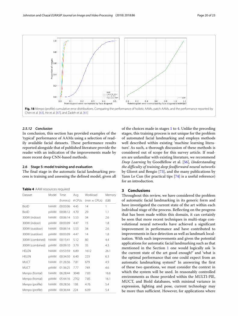
Johnston and Chazal EURASIP Journal on Image and Video Processing (2018) 2018:86 Page 20 of 23
Fig. 18Menpo (profile) cumulative error distributions. Comparing the performance of holistic AAMs, patch AAMs, and the performance reported byChen et al. [63], He et al. [67], and Zadeh et al. [61]
2.5.12 ConclusionIn conclusion, this section has provided examples of the‘typical’ performance of AAMs using a selection of read-ily available facial datasets. These performance resultsreported alongside that of published literature provide thereader with an indication of the improvements made bymore recent deep CNN-based methods.
2.6 Stage 5: model training and evaluationThe final stage in the automatic facial landmarking pro-cess is training and assessing the defined model, given all
Table 4 AAM resources required
Dataset Model Time Avg Workload Memory
(h:min:s) # CPUs (min × CPUs) (GB)
BioID hAAM 00:03:06 4.45 14 1
BioID pAAM 00:06:12 4.70 29 1.1
300W (indoor) hAAM 00:06:14 5.53 34 2.6
300W (indoor) pAAM 00:03:09 4.47 15 1.8
300W (outdoor) hAAM 00:06:14 5.53 34 2.6
300W (outdoor) pAAM 00:03:09 4.47 14 1.8
300W (combined) hAAM 00:15:41 5.12 80 4.4
300W (combined) pAAM 00:09:10 3.79 35 4.3
HELEN hAAM 03:53:59 6.89 1612 26.1
HELEN pAAM 00:34:50 6.40 223 6.3
MUCT hAAM 01:26:56 7.81 679 4.9
MUCT pAAM 01:36:25 7.77 749 4.6
Menpo (frontal) hAAM 06:28:44 3048 7.83 16.6
Menpo (frontal) pAAM 05:44:16 2702 7.85 16.1
Menpo (profile) hAAM 00:28:56 138 4.76 5.4
Menpo (profile) pAAM 00:36:44 224 6.09 5.4
of the choices made in stages 1 to 4. Unlike the precedingstages, this training process is not unique for the problemof automated facial landmarking and employs methodswell described within existing ‘machine learning litera-ture’. As such, a thorough discussion of these methods isconsidered out of scope for this survey article. If read-ers are unfamiliar with existing literature, we recommendDeep Learning by Goodfellow et al. [56], Understandingthe difficulty of training deep feedforward neural networksby Glorot and Bengio [73], and the many publications byYann Le Cun (for practical tips [74] is a useful reference)for an introduction.
3 ConclusionsThroughout this review, we have considered the problemof automatic facial landmarking in its generic form andhave investigated the current state of the art within eachindividual stage of the process. Reflecting on the progressthat has been made within this domain, it can certainlybe seen that more recent techniques in multi-stage con-volutional neural networks have achieved a significantimprovement in performance and have contributed toimprovements in face detection as well as landmark local-isation. With such improvements and given the potentialapplications for automatic facial landmarking such as thatmentioned in the Section 1 one would logically ask ‘isthe current state of the art good enough?’ and ‘what isthe optimal performance that one could expect from anautomatic landmarking system?’ In answering the firstof these two questions, we must consider the context inwhich the system will be used. In reasonably controlledenvironments as those provided within the MULTI-PIE,MUCT, and BioId databases, with minimal variance inexpression, lighting and pose, current technology maybe more than sufficient. However, for applications where

Johnston and Chazal EURASIP Journal on Image and Video Processing (2018) 2018:86 Page 21 of 23
these conditions would be highly variable such as attempt-ing to classify one’s mood in the outdoors using facialexpression, current technology may still struggle.Considering the optimal expected performance, it is our
opinion that the current best performing vision systemsare still biological. The vision system of humans is capableof accurately identifying facial characteristics given a veryhigh degree of variability in almost all aspects of an imageor ‘real-life’ situations. This differential in performanceis demonstrated by Sagonas et al. [10] which comparedthe landmarking variability of three expert annotators tothe automated methods of the 300W competition. Thehuman annotators outperformed the best automatic sys-tem by more than a factor of five (Table 3 [10]). In thecontext of extremely sophisticated applications such asautonomous cars, drones, and robots, a digital visionsystem with performance comparable to existing biolog-ical systems would be of enormous value. If the fieldis to achieve biological or near-biological performancein automated facial landmarking, we believe that addi-tional progress must be made in all five stages of modelconstruction described within this paper. Redefining theproblem objective as achieving near-biological system per-formance in facial landmarking, it is believed that the fieldwill require:
1 A significant increase in the availability of complex‘in-the-wild’ data sets with an extremely high samplesize, robust ground truth landmarks, and highvariability in facial pose, expression, degree ofobstruction, and lighting.
2 An improvement in the accuracy of face detectionmethods as well moving towards methods whichdescribe the outline of the face in more detail, ratherthan simply specifying the extent to which a face fitswithin a bounding box.
3 An improvement in modelling methods and learningtechniques which are able to capture thecharacteristics and variance within the datasets infine detail, without suffering from overfitting.
What is particularly interesting is that in previous years,this list would have included some increase in hardwarespecifications such as memory or processing power. How-ever, given the major increases in cloud computing anddistributed data processing, we do not consider comput-ing resources to be a significant current constraint. Cloudcomputing providers such as Amazon Web Services andGoogle Cloud Computing offer configurable instancesof CPUs, GPUs with extensible RAM which are readilyaccessible and at relatively low cost.
AbbreviationsAAM: Active appearance model; AdaGrad: Adaptive gradient algorithm; Adam:Adaptive moment estimation; ASM: Active shape model; CD-Net: Candidatedecision network; CE-CLM: Convolutional experts constrained local model;
CED: Cumulative error distribution; CEN: Convolutional experts network; CLM:Constrained local model; CNN: Convolutional neural network; CPU: Centralprocessing unit; DAN: Deep alignment network; DA-Net: Dataset acrossnetwork; FEC-CNN: Fully end to end cascaded convolutional neural network;GPU: Graphical processing unit; hAAM: Holistic active appearance model;HOG: Histogram of oriented gradients; NMRSE: Normalised root mean squarederror; OSA: Obstructive sleep apnoea; pAAM: Patch active appearance model;PDM: Point distribution model; RMSE: Root mean squared error; ROI: Region(s)of interest; SVM: Support vector machine
AcknowledgementsThe authors would like to thank the editors and anonymous reviewers for theirvaluable comments.
FundingNo funding has been provided for this work
Availability of data andmaterialsAll data, source code, and other materials used and generated for this articleare publicly available under a variety of open source licenses:
• Table 1 contains a list of publicly available facial landmarking datasets,including those used in the experimental components of this reviewpaper.
• The source code for all experimental components of this paper islicensed under GPL 3.0 and can be obtained from GitLab.
• Docker containers with executable forms of the source code are alsoavailable via DockerHub
• The image landmarking tool used for the ground truth varaibility study isalso available under GPL 3.0 on GitLab.
Authors’ contributionsBJ was responsible for the design, research, and writing of the paper as wellexecuting the experimental components. PC provided valuable assistance inplanning and preparing the experimental components, reviewing, shaping,and improving the quality of the final manuscript. Both authors read andapproved the final manuscript.
Authors’ informationBenjamin Johnston is a PhD candidate at the University of Sydney and a SeniorData Scientist at ResMed Ltd. Benjamin’s current research interests includecomputer vision, image processing, pattern recognition, and the applicationof these technologies in providing improved medical care.Professor Philip de Chazal is the ResMed Chair in Biomedical Engineering at theUniversity of Sydney. Professor de Chazal leads the University’s research andeducational activities in biomedical engineering, working across the CharlesPerkins Centre and the Faculty of Engineering and Information Technologies.
Competing interestsThe authors declare that they have no competing interests.
Publisher’s NoteSpringer Nature remains neutral with regard to jurisdictional claims inpublished maps and institutional affiliations.
Received: 27 December 2017 Accepted: 24 August 2018
References1. T. Wu, P. Turaga, R. Chellappa, Age estimation and face verification across
aging using landmarks. IEEE Trans. Inf. Forensic Secur. 7(6), 1780–1788(2012). https://doi.org/10.1109/TIFS.2012.2213812
2. T. Devries, K. Biswaranjan, G. W. Taylor, in 2014 Canadian Conference onComputer and Robot Vision. Multi-task learning of facial landmarks andexpression (IEEE, Montreal, 2014), pp. 98–103. https://doi.org/10.1109/CRV.2014.21, http://ieeexplore.ieee.org/document/6816830/
3. G. DL, J. Dusseldorp, H. TA, N. Jowett, A machine learning approach forautomated facial measurements in facial palsy. JAMA Facial Plast. Surg.20(4), 335 (2018). https://doi.org/10.1001/jamafacial.2018.0030

Johnston and Chazal EURASIP Journal on Image and Video Processing (2018) 2018:86 Page 22 of 23
4. S. Anping, X. Guoliang, D. Xuehai, S. Jiaxin, X. Gang, Z. Wu, Assessment forfacial nerve paralysis based on facial asymmetry. Australas. Phys. Eng. Sci.Med. 40(4), 851–860 (2017). https://doi.org/10.1007/s13246-017-0597-4
5. A. Tabatabaei Balaei, K. Sutherland, P. Cistulli, P. de Chazal, in 2017 IEEE14th International Symposium on Biomedical Imaging (ISBI 2017). Automaticdetection of obstructive sleep apnea using facial images, (Melbourne,2017), pp. 215–218. https://doi.org/10.1109/ISBI.2017.7950504
6. B. Johnston, A. McEwan, P. de Chazal, in 2017 39th Annual InternationalConference of the IEEE Engineering in Medicine and Biology Society (EMBC).Semi-automated nasal PAP mask sizing using facial photographs (IEEE,Jeju Island, 2017), pp. 1214–1217. https://doi.org/10.1109/EMBC.2017.8037049, http://ieeexplore.ieee.org/document/8037049/
7. O. Çeliktutan, S. Ulukaya, B. Sankur, A comparative study of facelandmarking techniques. EURASIP J. Image Video Process. 13, 1–27(2013). https://doi.org/10.1186/1687-5281-2013-13
8. F. Marcolin, E. Vezzetti, Novel descriptors for geometrical 3D face analysis.Multimedia Tools Appl. 76(12), 13805–13834 (2017). https://doi.org/10.1007/s11042-016-3741-3
9. E. Vezzetti, F. Marcolin, S. Tornincasa, L. Ulrich, N. Dagnes, 3Dgeometry-based automatic landmark localization in presence of facialocclusions. Multimedia Tools Appl. (2017). https://doi.org/10.1007/s11042-017-5025-y
10. C. Sagonas, E. Antonakos, G. Tzimiropoulos, S. Zafeiriou, M. Pantic, 300Faces In-The-Wild Challenge: database and results. Image Vis. Comput.47, 3–18 (2016). https://doi.org/10.1016/j.imavis.2016.01.002
11. C. Sagonas, G. Tzimiropoulos, S. Zafeiriou, M. Pantic, in 2013 IEEEInternational Conference on Computer VisionWorkshops. 300 Facesin-the-wild challenge: The first facial landmark localization challenge(IEEE, Sydney, 2013), pp. 397–403. https://doi.org/10.1109/ICCVW.2013.59,http://ieeexplore.ieee.org/document/6755925/
12. C. Sagonas, G. Tzimiropoulos, S. Zafeiriou, M. Pantic, in 2013 IEEE ComputerSociety Conference on Computer Vision and Pattern RecognitionWorkshops.A semi-automatic methodology for facial landmark annotation (IEEE,Portland, 2013), pp. 896–903. https://doi.org/10.1109/CVPRW.2013.132,http://ieeexplore.ieee.org/document/6595977/
13. Y. Wu, T. Hassner, K. Kim, G. Medioni, P. Natarajan, Facial landmarkdetection with tweaked convolutional neural networks. IEEE Trans.Pattern Anal. Mach. Intell (2015). https://doi.org/10.1109/TPAMI.2017.2787130, http://ieeexplore.ieee.org/document/8239860/
14. P. Viola, M. J. Jones, Robust real-time object detection. Int. J. Comput. Vis.February, 1–30 (2001). https://doi.org/10.1.1.23.2751
15. N. Dalal, B. Triggs, in 2005 IEEE Computer Society Conference on ComputerVision and Pattern Recognition (CVPR’05), vol.1. Histograms of orientedgradients for human detection (IEEE, San Diego, 2005), pp. 886–893.https://doi.org/10.1109/CVPR.2005.177, http://ieeexplore.ieee.org/document/1467360/
16. G. Bradski, OpenCV Library (2000). OpenCV.org. Accessed 5 Sept 201817. T. Li, W. Hou, F. Lyu, Y. Lei, C. Xiao, in 2016 Sixth International Conference on
InstrumentationMeasurement, Computer, Communication and Control(IMCCC). Face detection based on depth information using HOG-LBP(IEEE, Harbin, 2016), pp. 779–784. https://doi.org/10.1109/IMCCC.2016.92,http://ieeexplore.ieee.org/document/7774889/
18. F. Song, X. Tan, X. Liu, S. Chen, Eyes closeness detection from still imageswith multi-scale histograms of principal oriented gradients. PatternRecognit. 47(9), 2825–2838 (2014). https://doi.org/10.1016/j.patcog.2014.03.024
19. A. Suleiman, V. Sze, An energy-efficient hardware implementation ofHOG-based object detection at 1080HD 60 fps with multi-scale support.J. Signal Process. Syst. 84(3), 325–337 (2016). https://doi.org/10.1007/s11265-015-1080-7
20. R. Vaillant, C. Monrocq, Y. L. Cun, Original approach for the localisation ofobjects in images. IEE Proc. Vis. Image Signal Process. 141(4), 245–250(1994). https://doi.org/10.1049/ip-vis:19941301
21. M. Osadchy, Y. Le Cun, M. L. Miller, Synergistic face detection and poseestimation with energy-based models. J. Mach. Learn. Res. 8, 1197–1215(2007). https://doi.org/10.1007/11957959
22. Y. LeCun, L. Bottou, Y. Bengio, P. Haffner, Gradient-based learning appliedto document recognition. Proc. IEEE. 86(11), 2278–2323 (1998). https://doi.org/10.1109/5.726791. http://arxiv.org/abs/1102.0183
23. L. Haoxiang, L. Zhe, S. Xiaohui, J. Brandt, H. Gang, in 2015 IEEE Conferenceon Computer Vision and Pattern Recognition (CVPR). A convolutional neural
network cascade for face detection (IEEE, Boston, 2015), pp. 5325–5334.https://doi.org/10.1109/CVPR.2015.7299170
24. S. Yang, P. Luo, C. C. Loy, X. Tang, in 2016 IEEE Conference on ComputerVision and Pattern Recognition (CVPR). WIDER FACE: A face detectionbenchmark (IEEE, Las Vegas, 2016). https://doi.org/10.1109/CVPR.2016.596, http://ieeexplore.ieee.org/document/7780965/
25. X. Sun, P. Wu, S. C. H. Hoi, Face detection using deep learning: animproved faster RCNN approach. Neurocomputing. 299, 42–50 (2017)
26. R. Girshick, J. Donahue, T. Darrell, J. Malik, in 2014 IEEE Conference onComputer Vision and Pattern Recognition. Rich feature hierarchies foraccurate object detection and semantic segmentation (IEEE, Columbus,2014), pp. 580–587. https://doi.org/10.1109/CVPR.2014.81, http://ieeexplore.ieee.org/document/6909475/
27. M. Everingham, L. Van Gool, C. K. I. Williams, J. Winn, A. Zisserman, Thepascal visual object classes (voc) challenge. Int. J. Comput. Vis. 88(2),303–338 (2010)
28. R. Uijlings, A. van de Sande, T. Gevers, M. Smeulders, et al., selective searchfor object recognition. Int. J. Comput. Vis. 104(2), 154 (2013)
29. S. Bell, C. L. Zitnick, K. Bala, R. Girshick, in 2016 IEEE Conference on ComputerVision and Pattern Recognition (CVPR). Inside-outside net: detectingobjects in context with skip pooling and recurrent neural networks (IEEE,Las Vegas, 2016), pp. 2874–2883. http://doi.org/10.1109/CVPR.2016.314,http://ieeexplore.ieee.org/document/7780683/
30. S. Zhan, Q. Q. Tao, X. H. Li, Face detection using representation learning.Neurocomputing. 187, 1–8 (2015). https://doi.org/10.1016/j.neucom.2015.07.130
31. Q. Q. Tao, S. Zhan, X. H. Li, T. Kurihara, Robust face detection using localCNN and SVM based on kernel combination. Neurocomputing. 211,98–105 (2016). https://doi.org/10.1016/j.neucom.2015.10.139
32. D. Wang, J. Yang, J. Deng, Q. Liu, FaceHunter: A multi-task convolutionalneural network based face detector. Signal Process. Image Commun. 47,476–481 (2016). https://doi.org/10.1016/j.image.2016.04.004
33. S. Zafeiriou, C. Zhang, Z. Zhang, A survey on face detection in the wild:Past, present and future. Comp. Vision Image Underst. 138, 1–24 (2015).https://doi.org/10.1016/j.cviu.2015.03.015
34. M. Kawulok, M. E. Celebi, B. Smolka, Advances in Face Detection and FacialImage Analysis. (Springer, Cham, 2016). https://doi.org/10.1007/978-3-319-25958-1. http://link.springer.com/10.1007/978-3-319-25958-1
35. D. E. King, Dlib-ml: A Machine Learning Toolkit. J. Mach. Learn. Res. 10,1755–1758 (2009). https://doi.org/10.1145/1577069.1755843
36. A. Asthana, S. Zafeiriou, S. Cheng, M. Pantic, in 2014 IEEE Conference onComputer Vision and Pattern Recognition. Incremental face alignment inthe wild (IEEE, Columbus, 2014), pp. 1859–1866. https://doi.org/10.1109/CVPR.2014.240, http://ieeexplore.ieee.org/lpdocs/epic03/wrapper.htm?arnumber=6909636
37. J. Deng, Q. Liu, J. Yang, D. Tao, M3 CSR: Multi-view, multi-scale andmulti-component cascade shape regression. Image Vis. Comput. 47,19–26 (2015). https://doi.org/10.1016/j.imavis.2015.11.005
38. G. J. Edwards, C. J. Taylor, T. F. Cootes, in Proceedings Third IEEEInternational Conference on Automatic Face and Gesture Recognition.Interpreting face images using active appearance models (IEEE Comput.Soc, Nara, 1998), pp. 300–305. https://doi.org/10.1109/AFGR.1998.670965,http://ieeexplore.ieee.org/document/670965/
39. T. F. Cootes, G. J. Edwards, C. J. Taylor, active appearance models. IEEETrans. Pattern. Anal. Mach. Intell. 23(6), 681–685 (2001)
40. T. F. Cootes, C. J. Taylor, D. H. Cooper, J. Graham, Active shapemodels-Their training and application. Comp. Vision Image Underst.61(1), 38–59 (1995). https://doi.org/10.1006/cviu.1995.1004
41. J. C. Gower, Generalized procrustes analysis. Psychometrika. 40(1), 33–51(1975). https://doi.org/10.1007/BF02291478
42. K. Pearson, LIII. On lines and planes of closest fit to systems of points inspace. Philos. Mag. Ser. 6. 2(11), 559–572 (1901). https://doi.org/10.1080/14786440109462720
43. G. J. Edwards, C. J. Taylor, T. F. Cootes, in Proceedings - 3rd IEEE InternationalConference on Automatic Face and Gesture Recognition. Learning toidentify and track faces in image sequences (IEEE, Comput. Soc, Nara,1998), pp. 260–265. https://doi.org/10.1109/AFGR.1998.670958, http://ieeexplore.ieee.org/document/670958/
44. T. F. Cootes, C. J. Taylor, Statistical models of appearance for computervision. Technical report. (University of Manchester, Manchester, 2008).http://www.face-rec.org/algorithms/#AAMmodels.pdf

Johnston and Chazal EURASIP Journal on Image and Video Processing (2018) 2018:86 Page 23 of 23
45. T. Baltrusaitis, P. Robinson, L. P. P. Morency, in 2013 IEEE InternationalConference on Computer VisionWorkshops. Constrained local neural fieldsfor robust facial landmark detection in the wild, (2013), pp. 354–361.https://doi.org/10.1109/ICCVW.2013.54. http://ieeexplore.ieee.org/document/6755919/
46. D. Cristinacce, T. F. Cootes, in Procedings of the British Machine VisionConference. Feature detection and tracking with constrained local models(British Machine Vision Association, Edinburgh, 2006), pp. 95–19510.https://doi.org/10.5244/C.20.95
47. J. Peng, L. Bo, J. Xu, Conditional neural fields. Adv. Neural Inf. Process. Syst.9, 1–9 (2009)
48. J. Yan, Z. Lei, D. Yi, S. Z. Li, in Proceedingsof the IEEE International Conference onComputer Vision. Learn to combinemultiple hypotheses for accurate facealignment, (2013), pp. 392–396. https://doi.org/10.1109/ICCVW.2013.126
49. X. Xiong, F. De La Torre, Supervised descent method and its applicationsto face alignment. Proc. IEEE Comput. Soc. Conf. Comput. Vis. PatternRecognit., 532–539 (2013). https://doi.org/10.1109/CVPR.2013.75
50. D. G. Lowe, Distinctive image features from scale-invariant keypoints. Int.J. Comput. Vis. 60(2), 91–110 (2004). https://doi.org/10.1023/B:VISI.0000029664.99615.94. http://arxiv.org/abs/0112017
51. A. Krizhevsky, I. Sutskever, G. E. Hinton, ImageNet Classification with DeepConvolutional Neural Networks. Adv. Neural Inf. Process. Syst., 1–9 (2012).https://doi.org/10.1016/j.protcy.2014.09.007. http://arxiv.org/abs/1102.0183
52. L. Wan, M. Zeiler, S. Zhang, Y. L. Cun, R. Fergus, in Proceedings of the 30thInternational Conference onMachine Learning (ICML-13), vol. 28, ed. by S.Dasgupta, D. Mcallester. Regularization of neural networks usingDropConnect, (2013), pp. 1058–1066. http://jmlr.org/proceedings/papers/v28/wan13.pdf
53. A. Krizhevsky, Learningmultiple layers of features from tiny images.(University of Toronto, 2009), pp. 1–60. https://doi.org/10.1.1.222.9220.http://arxiv.org/abs/arXiv:1011.1669v3
54. B. Graham, Fractional Max-Pooling. International conference on learningrepresentations, 1–10 (2014). http://arxiv.org/abs/1412.6071
55. D.-A. Clevert, T. Unterthiner, S. Hochreiter, in International Conference onLearning Representations 2016 (ICLR 2016). Fast and accurate deep networklearning by exponential linear units (elus) (ICLR, San Juan, 2015), pp. 1–14.https://arxiv.org/abs/1511.07289
56. I. Goodfellow, Y. Bengio, A. Courville, in Deep Learning. ConvolutionalNetworks (MIT Press, Cambridge, 2016), pp. 330–372. http://www.deeplearningbook.org
57. S. Zafeiriou, G. Trigeorgis, G. Chrysos, J. Deng, J. Shen, in 2017 IEEEConference on Computer Vision and Pattern RecognitionWorkshops(CVPRW). The Menpo Facial Landmark Localisation Challenge: A StepTowards the Solution (IEEE, Honolulu, 2017). https://doi.org/10.1109/CVPRW.2017.263. http://ieeexplore.ieee.org/document/8014997/
58. E. Zhou, H. Fan, Z. Cao, Y. Jiang, Q. Yin, in 2013 IEEE InternationalConference on Computer VisionWorkshops. Extensive facial landmarklocalization with coarse-to-fine convolutional network cascade(Institute of Electrical and Electronics Engineers Inc., Sydney, 2013),pp. 386–391
59. H. Fan, E. Zhou, Approaching human level facial landmark localization bydeep learning. Image Vision Comput. Online J. 47, 27–35 (2016). https://doi.org/10.1016/j.imavis.2015.11.004
60. J. Yang, Q. Liu, K. Zhang, in The IEEE Conference on Computer Vision andPattern Recognition (CVPR) Workshops. Stacked hourglass network forrobust facial landmark localisation, (2017)
61. A. Zadeh, T. Baltrusaitis, L. P. Morency, in The IEEE Conference on ComputerVision and Pattern Recognition (CVPR) Workshops. Convolutional expertsconstrained local model for facial landmark detection, (2017)
62. Y. Sun, X. Wang, X. Tang, in Proceedings of the IEEE Computer SocietyConference on Computer Vision and Pattern Recognition. Deepconvolutional network cascade for facial point detection, (2013),pp. 3476–3483. https://doi.org/10.1109/CVPR.2013.446
63. X. Chen, E. Zhou, Y. Mo, J. Liu, Z. Cao, in The IEEE Conference on ComputerVision and Pattern Recognition (CVPR) Workshops. Delving deep intocoarse-to-fine framework for facial landmark localization, (2017)
64. C. Zhang, Z. Zhang, in 2014 IEEEWinter Conference on Applications ofComputer Vision, WACV 2014. Improving multiview face detection withmulti-task deep convolutional neural networks, (2014), pp. 1036–1041.https://doi.org/10.1109/WACV.2014.6835990
65. A. Newell, K. Yang, J. Deng, Stacked hourglass networks for human poseestimation. Eur. Conf. Comput. Vis., 483–499 (2016). https://doi.org/10.1007/978-3-319-46484-8. http://arxiv.org/abs/1603.06937
66. W. Wu, S. Yang, in The IEEE Conference on Computer Vision and PatternRecognition (CVPR) Workshops. Leveraging intra and inter-datasetvariations for robust face alignment, (2017)
67. Z. He, M. Kan, J. Zhang, X. Chen, S. Shan, in 2017 12th IEEE InternationalConference on Automatic Face & Gesture Recognition (FG 2017). A fullyend-to-end cascaded CNN for facial landmark detection (IEEE,Washington, D.C, 2017), pp. 200–207. https://doi.org/10.1109/FG.2017.33
68. Z. He, J. Zhang, M. Kan, S. Shan, X. Chen, in 2017 IEEE Conference onComputer Vision and Pattern RecognitionWorkshops (CVPRW). RobustFEC-CNN: A high accuracy facial landmark detection system (IEEE,Honolulu, 2017). http://doi.org/10.1109/CVPRW.2017.255. http://ieeexplore.ieee.org/document/8014989/
69. J. M. Saragih, S. Lucey, J. F. Cohn, Deformable model fitting by regularizedlandmark mean-shift. Int. J. Comput. Vis. 91(2), 200–215 (2011). https://doi.org/10.1007/s11263-010-0380-4
70. M. Kowalski, J. Naruniec, T. Trzcinski, in The IEEE Conference on ComputerVision and Pattern Recognition (CVPR)Workshops. Deep alignment network:A convolutional neural network for robust face alignment, (2017)
71. C. Sagonas, S. Zafeiriou, Facial point annotations (2017). https://ibug.doc.ic.ac.uk/resources/facial-point-annotations/ Accessed 18 May 2017
72. S. Milborrow, T. E. Bishop, F. Nicolls, in Proceedings of the IEEE InternationalConference on Computer Vision. Multiview active shape models with SIFTdescriptors for the 300-W face landmark challenge, (2013), pp. 378–385.https://doi.org/10.1109/ICCVW.2013.57
73. X. Glorot, Y. Bengio, Understanding the difficulty of training deepfeedforward neural networks. Proc. 13th Int. Conf. Artif. Intell. Stat.(AISTATS). 9, 249–256 (2010). https://doi.org/10.1.1.207.2059
74. Y. LeCun, G. Montavon, G. B. Orr, K. R. Mülle, Y. LeCun, in Neural Networks:Tricks of the Trade. Lecture Notes in Computer Science, vol. 7700, ed. by.G. Montavon, G. B. Orr, and K. R. Müller. Efficient BackProp (Springer, Berlin,Heidelberg, 2012), pp. 9–48. https://doi.org/10.1007/978-3-642-35289-8
75. R. Gross, I. Matthews, J. Cohn, T. Kanade, S. Baker, in 2008 8th IEEEInternational Conference on Automatic Face Gesture Recognition. Multi-PIE,(2008), pp. 1–8. https://doi.org/10.1109/AFGR.2008.4813399
76. S. Milborrow, J. Morkel, F. Nicolls, The MUCT landmarked face database.Pattern Recog. Assoc. S. Afr. (2010)
77. K. Messer, J. Matas, J. Kittler, J. Luettin, G. Maitre, in Second InternationalConference on Audio and Video-based Biometric Person Authentication, vol.964. XM2VTSDB: The extended M2VTS database (AVBPR, Washington, D.C,1999), pp. 965–966
78. S. Zafeiriou, M. Pantic, G. Chrysos, G. Trigeorgis, J. Deng, J. Shen, 2nd faciallandmark localisation competition - The Menpo benchMark (2017)
79. M. Koestinger, P. Wohlhart, P. M. Roth, H. Bischof, in 2011 IEEE InternationalConference on Computer VisionWorkshops (ICCVWorkshops). Annotatedfacial landmarks in the wild: A large-scale, real-world database for faciallandmark localization, (2011). https://doi.org/10.1109/ICCVW.2011.6130513. http://ieeexplore.ieee.org/document/6130513/
80. A. Kasinski, A. Florek, A. Schmidt, The PUT face database. Image Process.Commun. 13(3-4), 59–64 (2008)
81. M. Fink, R. Fergus, A. Angelova, Caltech 10,000 web faces (2007). http://www.vision.caltech.edu/Image_Datasets/Caltech_10K_WebFaces/
82. O. Jesorsky, K. J. Kirchberg, R. W. Frischholz, in International Conference onAudio-and Video-Based Biometric Person Authentication. Robust facedetection using the hausdorff distance (Springer, 2001), pp. 90–95
83. V. Le, J. Brandt, Z. Lin, L. Bourdev, T. S. Huang, in European Conference onComputer Vision - ECCV 2012, Lecture Notes in Computer Science), vol. 7574LNCS. Interactive facial feature localization (Springer, Berlin, 2012),pp. 679–692. https://doi.org/10.1007/978-3-642-33712-349. http://link.springer.com/10.1007/978-3-642-33712-349
84. G. B. Huang, M. Mattar, T. Berg, E. Learned-Miller, inWorkshop on facesin’Real-Life’Images: detection, alignment, and recognition. Labeled faces inthe wild: A database forstudying face recognition in unconstrainedenvironments, (2008)
Related Documents