A Representation Learning Framework for Property Graphs

A Representation Learning Framework for Property GraphsYifan Hou, Hongzhi Chen, Changji Li, James Cheng, Ming-Chang Yang

Department of Computer Science and EngineeringThe Chinese University of Hong Kong

{yfhou,hzchen,cjli,jcheng,mcyang}@cse.cuhk.edu.hk

ABSTRACTRepresentation learning on graphs, also called graph embedding,has demonstrated its significant impact on a series of machinelearning applications such as classification, prediction and recom-mendation. However, existing work has largely ignored the richinformation contained in the properties (or attributes) of both nodesand edges of graphs in modern applications, e.g., those representedby property graphs. To date, most existing graph embedding meth-ods either focus on plain graphs with only the graph topology, orconsider properties on nodes only. We propose PGE, a graph repre-sentation learning framework that incorporates both node and edgeproperties into the graph embedding procedure. PGE uses nodeclustering to assign biases to differentiate neighbors of a node andleverages multiple data-driven matrices to aggregate the propertyinformation of neighbors sampled based on a biased strategy. PGEadopts the popular inductive model for neighborhood aggregation.We provide detailed analyses on the efficacy of our method andvalidate the performance of PGE by showing how PGE achievesbetter embedding results than the state-of-the-art graph embeddingmethods on benchmark applications such as node classification andlink prediction over real-world datasets.

KEYWORDSgraph neural networks, graph embedding, property graphs, repre-sentation learning

ACM Reference Format:Yifan Hou, Hongzhi Chen, Changji Li, James Cheng, Ming-Chang Yang.2019. A Representation Learning Framework for Property Graphs. In The25th ACM SIGKDD Conference on Knowledge Discovery and Data Mining(KDD ’19), August 4–8, 2019, Anchorage, AK, USA. ACM, New York, NY, USA,9 pages. https://doi.org/10.1145/3292500.3330948

1 INTRODUCTIONGraphs are ubiquitous today due to the flexibility of using graphs tomodel data in a wide spectrum of applications. In recent years, moreand more machine learning applications conduct classification orprediction based on graph data [7, 15, 17, 28], such as classifyingprotein’s functions in biological graphs, understanding the rela-tionship between users in online social networks, and predicting

Permission to make digital or hard copies of all or part of this work for personal orclassroom use is granted without fee provided that copies are not made or distributedfor profit or commercial advantage and that copies bear this notice and the full citationon the first page. Copyrights for components of this work owned by others than ACMmust be honored. Abstracting with credit is permitted. To copy otherwise, or republish,to post on servers or to redistribute to lists, requires prior specific permission and/or afee. Request permissions from [email protected] ’19, August 4–8, 2019, Anchorage, AK, USA© 2019 Association for Computing Machinery.ACM ISBN 978-1-4503-6201-6/19/08. . . $15.00https://doi.org/10.1145/3292500.3330948

purchase patterns in buyers-products-sellers graphs in online e-commerce platforms. However, it is not easy to directly make useof the structural information of graphs in these applications asgraph data are high-dimensional and non-Euclidean. On the otherhand, considering only graph statistics such as degrees [6], kernelfunctions [14], or local neighborhood structures [24] often provideslimited information and hence affects the accuracy of classifica-tion/prediction.

Representation learning methods [5] attempt to solve the above-mentioned problem by constructing an embedding for each nodein a graph, i.e., a mapping from a node to a low-dimensional Eu-clidean space as vectors, which uses geometric metrics (e.g., Eu-clidean distance) in the embedding space to represent the struc-tural information. Such graph embeddings [15, 17] have achievedgood performance for classification/prediction on plain graphs (i.e.,graphs with only the pure topology, without node/edge labels andproperties). However, in practice, most graphs in real-world do notonly contain the topology information, but also contain labels andproperties (also called attributes) on the entities (i.e., nodes) andrelationships (i.e., edges). For example, in the companies that wecollaborate with, most of their graphs (e.g., various graphs relatedto products, buyers and sellers from an online e-commerce platform;mobile phone call networks and other communication networksfrom a service provider) contain rich node properties (e.g., user pro-file, product details) and edge properties (e.g., transaction records,phone call details). We call such graphs as property graphs. Ex-isting methods [10, 16, 18, 22, 30, 31, 36] have not considered totake the rich information carried by both nodes and edges into thegraph embedding procedure.

This paper studies the problem of property graph embedding.There are two main challenges. First, each node v may have manyproperties and it is hard to find which properties may have greaterinfluence on v for a specific application. For example, consider theclassification of papers into different topics for a citation graphwhere nodes represent papers and edges model citation relation-ships. Suppose that each node has two properties, “year” and “title”.Apparently, the property “title” is likely to be more important forpaper classification than the property “year”. Thus, how to measurethe influence of the properties on each node for different applica-tions needs to be considered. Second, for each nodev , its neighbors,as well as the connecting edges, may have different properties. Howto measure the influences of both the neighbors and the connectingedges on v for different application poses another challenge. In theabove example, for papers referencing a target paper, those withhigh citations should mean more to the target paper than thosewith low citations.

Among existing work, GCN [22] leverages node property infor-mation for node embedding generation, while GraphSAGE [18]extends GCN from a spectral method to a spatial one. Given an

Research Track Paper KDD ’19, August 4–8, 2019, Anchorage, AK, USA

65

application, GraphSAGE trains a weight matrix before embeddingand then aggregates the property information of the neighborsof each node with the trained matrix to compute the node em-bedding. However, GraphSAGE does not differentiate neighborswith property dissimilarities for each node, but rather treats allneighbors equally when aggregating their property information.Moreover, GraphSAGE considers only node information and ig-nores edge directions and properties. Apart from the properties onnodes/edges, real-world graphs also have special structural features.For example, in social networks, nodes are often organized in theform of communities, where similar nodes are either neighbors dueto the homophily feature [3, 4], or not direct neighbors but withsimilar structure due to the structural equivalent feature [13, 19, 37].Thus, it is important to also consider structural features. For that,node2vec [16] learns node embeddings by combining two strate-gies, breadth-first random walk and depth-first random walk, toaccount for the homophily feature and structural equivalent fea-ture. However, node2vec only utilizes these two structural featureswithout considering any property information.

To address the limitations of existing methods, we propose anew framework, PGE, for property graph embedding. PGE appliesa biased method to differentiate the influences of the neighborsand the corresponding connecting edges by incorporating boththe topology and property information into the graph embeddingprocedure. The framework consists of three main steps: (1) property-based node clustering to classify the neighborhood of a node intosimilar and dissimilar groups based on their property similaritywith the node; (2) biased neighborhood sampling to obtain a smallerneighborhood sampled according the bias parameters (which are setbased on the clustering result), so that the embedding process canbe more scalable; and (3) neighborhood aggregation to compute thefinal low dimensional node embeddings by aggregating the propertyinformation of sampled neighborhood with weight matrices trainedwith neural networks.We also analyze in details how the three stepswork together to contribute to a good graph embedding and whyour biased method (incorporating node and edge information) canachieve better embedding results than existing methods.

We validated the performance of PGE by comparing with repre-sentative graph embedding methods, including DeepWalk [30] andnode2vec [16] representing random walk based methods, GCN [22]for graph convolutional networks, and GraphSAGE [18] for neighboraggregation based on weight matrices. We tested these methods fortwo benchmark applications, node classification and link predic-tion, on a variety of real-world graphs. The results show that PGEachieves significant performance improvements over these existingmethods. The experimental evaluation validates the importanceof incorporating node/edge property information, in addition totopology information, into graph embedding. It also demonstratesthe effectiveness of our biased strategy that differentiates neighborsto obtain better embedding results.

2 RELATEDWORKThere are three main methods for graph embedding: matrix factor-ization, random walk, and neighbors aggregation.

For matrix factorization methods, [2, 8] use adjacency matrixto define and measure the similarity among nodes for graph em-bedding. HOPE [29] further preserves high-order proximities andobtains asymmetric transitivity for directed graphs. Another line ofworks utilize the random walk statistics to learn embeddings withthe skip-gram model [26], which applies vector representation tocapture word relationships.

The key idea of random walk is that nodes usually tend to co-occur on short random walks if they have similar embeddings [17].DeepWalk [30] is the first to input random walk paths into a skip-gram model for learning node embeddings. node2vec [16] furtherutilizes biased random walks to improve the mapping of nodesto a low-dimensional space, while combining breadth-first walksand depth-first walks to consider graph homophily and structuralequivalence. To obtain larger relationships, Walklets [31] involvesoffset to allow longer step length during a random walk, whileHARP [10] makes use of graph preprocessing that compresses somenodes into one super-node to improve random walk.

According to [17],matrix factorization and randomwalkmethodsare shallow embedding approaches and have the following draw-backs. First, since the node embeddings are independent and thereis no sharing of parameters or functions, these methods are notefficient for processing large graphs. Second, they do not considernode/edge properties. Third, as the embeddings are transductiveand can only be generated during the training phrase, unseen nodescannot be embedded with the model being learnt so far.

To address (some of) the above problems, graph-based neuralnetworks have been used to learn node embeddings, which en-code nodes into vectors by compressing neighborhood informa-tion [9, 20, 36]. However, although this type of methods can shareparameters, strictly speaking they are still transductive and haveperformance bottlenecks for processing large graphs as the inputdimensionality of auto-encoders is equal to the number of nodes.Several recent works [11, 18, 22, 23, 34] attempted to use only localneighborhood instead of the entire graph to learn node embeddingsthrough neighbor aggregation, which can also consider propertyinformation on nodes. GCN [22] uses graph convolutional networksto learn node embeddings, by merging local graph structures andfeatures of nodes to obtain embeddings from the hidden layers.GraphSAGE [18] is inductive and able to capture embeddings forunseen nodes through its trained auto-encoders directly. The ad-vantage of neighborhood aggregation methods is that they not onlyconsider the topology information, but also compute embeddingsby aggregating property vectors of neighbors. However, existingneighborhood aggregation methods treat the property informationof neighbors equally and fail to differentiate the influences of neigh-bors (and their connecting edges) that have different properties.

3 THE PGE FRAMEWORKWe use G = {V, E,P,L} to denote a property graph , where Vis the set of nodes and E is the set of edges. P is the set of allproperties and P = PV ∪ PE , where PV =

⋃v ∈V {pv }, PE =⋃

e ∈E {pe }, and pv and pe are the set of properties of node v andedge e , respectively. L = LV ∪ LE is the set of labels, whereLV and LE are the sets of node and edge labels, respectively.We use Nv to denote the set of neighbors of node v ∈ V , i.e.,

Research Track Paper KDD ’19, August 4–8, 2019, Anchorage, AK, USA

66

Nv = {v ′ : (v,v ′) ∈ E}. In the case that G is directed, we mayfurther define Nv as the set of in-neighbors and the set of out-neighbors, though in this paper we abuse the notation a bit anddo not use new notations such as N in

v and Noutv for simplicity of

presentation, as the meaning should be clear from the context.The property graph model is general and can represent other

popular graph models. If we set P = ∅ and L = ∅, then G becomesa plain graph, i.e., a graph with only the topology. If we setPV = A,PE = ∅, and L = ∅, where A is the set of node attributes, thenG becomes an attributed graph. If we set L = LV , P = ∅, andLE = ∅, then G is a labeled graph.

3.1 Problem DefinitionThe main focus of PGE is to utilize both topology and property in-formation in the embedding learning procedure to improve theresults for different applications. Given a property graph G =

{V, E,P,L}, we define the similarity between two nodes vi ,vj ∈V as sG(vi ,vj ). The similarity can be further decomposed intotwo parts, sG(vi ,vj ) = l(sP (vi ,vj ), sT (vi ,vj )), where sP (vi ,vj )is the property similarity and sT (vi ,vj ) is the topology similaritybetween vi and vj , and l(·, ·) is a non-negative mapping.

The embedding of nodev ∈ V is denoted as zv , which is a vectorobtained by an encoder ENC(v) = zv . Our objective is to find theoptimal ENC(·), which minimizes the gap

∑vi ,vj ∈V | |sG(vi ,vj ) −

z⊤vi zvj | |=∑vi ,vj ∈V | |l(sP (vi ,vj ), sT (vi ,vj )) − z⊤vi zvj | |.

From the above problem definition, it is apparent that only con-sidering the topology similarity sT (vi ,vj ), as the traditional ap-proaches do, cannot converge to globally optimal results. In addi-tion, given a nodev and its neighborsvi ,vj , the property similaritysP (v,vi ) can be very different from sP (v,vj ). Thus, in the PGEframework, we use both topology similarity and property similarityin learning the node embeddings.

3.2 The Three Steps of PGEThe PGE framework consists of three major steps as follows.

• Step 1: Property-based Node Clustering. We cluster nodes inG based on their properties to producek clustersC={C1,C2, ...,Ck }.A standard clustering algorithm such as K-Means [25] or DB-SCAN [12] can be used for this purpose, where each node to beclustered is represented by its property vector (note that graphtopology information is not considered in this step).

• Step 2: Biased Neighborhood Sampling. To combine the influ-ences of property information and graph topology by l(·, ·), weconduct biased neighborhood sampling based on the results ofclustering in Step 1. To be specific, there are two phases in thisstep: (1) For each neighbor v ′ ∈ Nv , if v ′ and v are in the samecluster, we assign a bias bs to v ′ to indicate that they are similar;otherwise we assign a different bias bd to v ′ instead to indicatethat they are dissimilar. (2) We normalize the assigned biaseson Nv , and then sample Nv according to the normalized biasesto obtain a fixed-size sampled neighborhood Ns

v .• Step 3: Neighborhood Aggregation. Based on the sampledneighborsNs

v in Step 2, we aggregate their property informationto obtain zv by multiplying the weight matrices that are trainedwith neural networks.

In the following three sub-sections, we discuss the purposes anddetails of each of the above three steps.

3.2.1 Property-based Node Clustering. The purpose of Step 1 is toclassify Nv into two types for each node v based on their nodeproperty information, i.e., those similar to v or dissimilar to v . If vand its neighbor v ′ ∈ Nv are in the same cluster, we will regard v ′

as a similar neighbor of v . Otherwise, v ′ is dissimilar to v .Due to the high dimensionality and sparsity of properties (e.g.,

property values are often texts but can also be numbers and othertypes), which also vary significantly from datasets to datasets, it isnot easy to classify the neighborhood of each node into similar anddissimilar groups while maintaining a unified global standard forclassifying the neighborhood of all nodes. For example, one mightattempt to calculate the property similarity between v and each ofv’s neighbors, for all v ∈ V , and then set a threshold to classify theneighbors into similar and dissimilar groups. However, differentnodes may require a different threshold and their similarity rangescan be very different. Moreover, each node’s neighborhood may beclassified differently and as we will show later, the PGE frameworkactually uses the 2-hop neighborhood while this example onlyconsiders the 1-hop neighborhood. Thus, we need a unified globalstandard for the classification. For this purpose, clustering the nodesbased on their properties allows all nodes to be classified based onthe same global standard. For example, the 1-hop neighbors and the2-hop neighbors of a node v are classified in the same way basedon whether they are in the same cluster as v .

3.2.2 Biased Neighborhood Sampling. Many real-world graphshave high-degree nodes, i.e., these nodes have a large number ofneighbors. It is inefficient and often unnecessary to consider all theneighbors for neighborhood aggregation in Step 3. Therefore, weuse the biases bs and bd to derive a sampled neighbor set Ns

v witha fixed size for each node v . As a result, we obtain a sampled graphGs = {V, Es }, where Es = {(v,v ′) : v ′ ∈ Ns

v }. Since the biases bsand bd are assigned to the neighbors based on the clustering resultscomputed from the node properties, Gs contains the topology in-formation of G while it is constructed based on the node propertyinformation. Thus, Step 2 is essentially a mapping l(·, ·) that fusessP (v,v

′) and sT (v,v ′).The biases bs and bd are the un-normalized possibility of se-

lecting neighbors from dissimilar and similar clusters, respectively.The value of bs is set to 1, while bd can be varied depending on theprobability (greater bd means higher probability) that dissimilarneighbors should be selected into Gs . We will analyze the effectsof the bias values in Section 4 and verify by experimental resultsin Section 5.3.2. The size of Ns

v is set to 25 by default followingGraphSAGE [18] (also for fair comparison in our experiments). Thesize 25 was found to be a good balance point in [18] as a largersize will significantly increase the model computation time, thoughin the case of PGE as it differentiates neighbors, using a sampledneighborhood could achieve a better quality of embedding thanusing the full neighborhood.

3.2.3 Neighborhood Aggregation. The last step is to learn the lowdimensional embedding with Gs = {V, Es }. We use neighborhoodaggregation to learn the function ENC(·) for generating the nodeembeddings. For each node, we select its neighbors within two hops

Research Track Paper KDD ’19, August 4–8, 2019, Anchorage, AK, USA

67

to obtain zv by the following equations:

zv = σ (W 1 · A(z1v ,∑

v ′∈Nsv

z1v ′/|Nsv |)),

z1v ′ = σ (W 2 · A(pv ′ ,∑

v ′′∈Nsv′

pv ′′/|Nsv ′ |)),

where pv is the original property vector of node v , σ (·) is the non-linear activation function and A(·) is the concatenate operation. Weuse two weight matricesW 1 andW 2 to aggregate the node propertyinformation of v’s one-hop neighbors and two-hop neighbors.

The matrixW i is used to assign different weights to differentproperties because aggregating (e.g., taking mean value) node prop-erty vectors directly cannot capture the differences between prop-erties, but different properties contribute to the embedding in vary-ing degrees. Also, the weight matrix is data-driven and shouldbe trained separately for different datasets and applications, sincenodes in different graphs have different kinds of properties. Theweight matrices are pre-trained using Adam SGD optimizer [21],with a loss function defined for the specific application, e.g., for nodeclassification, we use binary cross entropy loss (multi-labeled); forlink prediction, we use cross entropy loss with negative sampling.

3.3 Support of Edge Direction and PropertiesThe sampled graph Gs does not yet consider the edge directionand edge properties. To include edge properties, we follow thesame strategy as we do on nodes. If edges are directed, we con-sider in-edges and out-edges separately. We cluster the edges intoke clusters Ce = {Ce

1 ,Ce2 , ...,C

eke }. Then, we train 2 · ke matrices,

{W 11 ,W

12 , ...,W

1ke } and {W 2

1 ,W22 , ...,W

2ke }, to aggregate node prop-

erties for ke types of edges for the 2-hop neighbors. Finally, weobtain zv by the following equations:

zv =σ(A(W 1

0 · z1v ,ACei ∈C

e (W 1i · Ev ′∈Ns

v& (v,v ′)∈Cei[z1v ′])

) ), (1)

z1v ′ =σ(A(W 2

0 ·pv ′ ,ACei ∈C

e (W 2i ·Ev ′′∈Ns

v′& (v ′,v ′′)∈Cei[pv ′′])

) ). (2)

Note that |Ce | should not be too large as to avoid high-dimensionalvector operations. Also, if |Ce | is too large, some clusters maycontain only a few elements, leading to under-fitting for the trainedweight matrices. Thus, we set |Ce | as a fixed small number.

3.4 The AlgorithmAlgorithm 1 presents the overall procedure of computing the em-bedding vector zv of each node v ∈ V . The algorithm followsexactly the three steps that we have described in Section 3.2.

4 AN ANALYSIS OF PGEIn this section, we present a detailed analysis of PGE. In particular,we analyze why the biased strategy used in PGE can improve theembedding results. We also discuss how the bias values bd and bsand edge information affect the embedding performance.

4.1 The Efficacy of the Biased StrategyOne of the main differences between PGE and GraphSAGE [18]is that neighborhood sampling in PGE is biased (i.e., neighborsare selected based on probability values defined based on bd and

Algorithm 1 Property Graph Embedding (PGE)Input: A Property Graph G = {V, E, P}; biases bd and bs ; the size

of sampled neighborhood |Nsv |; weight matrices {W 1

1 ,W12 , ...,W

1ke }

and {W 21 ,W

22 , ...,W

2ke }

Output: Low-dimensional representation vectors zv , ∀v ∈ V

1: Clustering V , E, and obtain C and Ce based on P; ▷ step 12: for all v ∈ V do ▷ step 23: for all v ′ ∈ Nv do4: Assign b = bd + (bs − bd ) ·

∑Ci ∈C I{v, v

′ ∈ Ci } to v ′,5: where I{v, v ′ ∈ Ci } = 1 if v, v ′ ∈ Ci and 0 otherwise;6: end for7: Sample |Ns

v | neighbors with bias b ;8: end for9: for all v ∈ V do ▷ step 310: Compute z1v with Equation (2);11: end for12: for all v ∈ V do13: Compute zv with Equation (1);14: end for

bs ), while GraphSAGE’s neighborhood sampling is unbiased (i.e.,neighbors are sampled with equal probability). We analyze thedifference between the biased and the unbiased strategies in thesubsequent discussion.

We first argue that neighborhood sampling is a special caseof random walk. For example, if we set the walk length to 1 andperform 10 times of walk, the strategy can be regarded as 1-hopneighborhood sampling with a fixed size of 10. Considering thatthe random walk process in each step follows an i.i.d. process forall nodes, we define the biased strategy as a |V| × |V| matrix P,where Pi, j is the probability that node vi selects its neighbor vj inthe random walk. If two nodes vi and vj are not connected, thenPi, j = 0. Similarly, we define the unbiased strategy Q, where allneighbors of any node have the same probability to be selected. Wealso assume that there exists an optimal strategy B, which givesthe best embedding result for a given application.

A number of works [10, 16, 31] have already shown that addingpreference on similar and dissimilar neighbors during random walkcan improve the embedding results, based on which we have thefollowing statement: for a biased strategy P, if | |B−P| |1 < | |B−Q| |1,where B , Q, then P has a positive influence on improving theembedding results.

Thus, to verify the efficacy of PGE’s biased strategy, we need toshow that our strategy P satisfies | |B − P| |1 ≤ ||B − Q| |1. To do so,we show that bd and bs can be used to adjust the strategy P to getcloser to B (than Q).

Assume that nodes are classified intok clustersC = {C1,C2, ...,Ck }based on the property information PV . For the unbiased strategy,the expected similarity of two nodes v,v ′ ∈ V for each randomwalk step is:

E[sG(v,v ′)] =

∑v ∈V

∑vi ∈Nv sG(v,vi )

|E |.

The expectation of two nodes’ similarity for each walk step in ourbiased strategy is:

E[sG(v,v ′)] =

∑v ∈V

∑vi ∈Nv∩Cv ns (v) · sG(v,vi )

|E |

k

Research Track Paper KDD ’19, August 4–8, 2019, Anchorage, AK, USA

68

+

∑v ∈V

∑vj ∈Nv∩(Cv )c nd (v) · sG(v,vj )

|E | ·(k−1)k

, (3)

where ns (v) and nd (v) are the normalized biases of bs and bd fornode v respectively, Cv is the cluster that contains v , and (Cv )

c =

C\{Cv }. Since only connected nodes are to be selected in a randomwalk step, the normalized biases ns (v) and nd (v) can be derived by

ns (v) =bs

bd ·∑v ′∈Nv I{v

′ ∈ Cv } + bs ·∑v ′∈Nv I{v

′ ∈ (Cv )c },

andnd (v) = ns (v) ×

bdbs.

Consider Equation (3), if we set bd = bs , which means nd (v) =ns (v), then it degenerates to the unbiased random walk strategy.But if we set bd and bs differently, we can adjust the biased strategyto either (1) select more dissimilar neighbors by assigning bd > bsor (2) select more similar neighbors by assigning bs > bd .

Assume that the clustering result is not trivial, i.e., we obtain atleast more than 1 cluster, we can derive that∑

Ci ∈C∑v,v ′∈Ci sP (v,v

′)

12∑Ci ∈C |Ci | · (|Ci | − 1)

>

∑v,v ′∈V sP (v,v

′)

12 |V | · (|V | − 1)

.

Since l(·, ·) is a non-negative mapping with respect to sP (v,v ′), wehave ∑

Ci ∈C∑v,v ′∈Ci sG(v,v

′)

12∑Ci ∈C |Ci | · (|Ci | − 1)

>

∑v,v ′∈V sG(v,v

′)

12 |V | · (|V | − 1)

(4).

Equation (4) shows that the similarity sG(v,v ′) is higher if v andv ′ are in the same cluster. Thus, based on Equations (3) and (4), weconclude that parameters bd and bs can be used to select similarand dissimilar neighbors.

Next, we consider the optimal strategy B for 1-hop neighbors,where Bi, j = I{vj ∈ Nvi } · b

∗vi ,vj , and b∗vi ,vj is the normalized

optimal bias value forBi, j . Similarly, the unbiased strategy isQi, j =

I{vj ∈ Nvi } ·1

|Nvi |. Thus, we have

| |B − Q| |1 =∑

vi ∈V

∑vj ∈V

���b∗vi ,vj − 1|Nvi |

���.For our biased strategy, Pi, j = I{vj ∈ Nvi ∩ Cvi } · ns (v) +

I{vj ∈ Nvi ∩ (Cvi )c } · nd (v). There exist bs and bd that satisfy∑

vi ∈V∑vj ∈V

���b∗vi ,vj − 1|Nvi |

��� ≥ ∑vi ∈V

∑vj ∈V

���b∗vi ,vj − I{vj ∈Nvi ∩ Cvi } · ns (v) − I{vj ∈ Nvi ∩ (Cvi )

c } · nd (v)���, where strict

inequality can be derived if bd , bs . Thus, | |B − P| |1 < | |B − Q| |1if we set proper values for bs and bd (we discuss the bias values inSection 4.2). Without loss of generality, the above analysis can beextended to the case of multi-hop neighbors.

4.2 The Effects of the Bias ValuesNext we discuss how to set the proper values for the biases bs andbd for neighborhood sampling. We also analyze the impact of thenumber of clusters on the performance of PGE.

For neighborhood aggregation in Step 3 of PGE, an accurateembedding of a node v should be obtained by covering the wholeconnected component that contains v , where all neighbors withink-hops (k is the maximum reachable hop) should be aggregated.

However, for a large graph, the execution time of neighborhoodaggregation increases rapidly beyond 2 hops, especially for power-law graphs. For this reason, we trade accuracy by considering onlythe 2-hop neighbors. In order to decrease the accuracy degradation,we can enlarge the change that a neighbor can contribute to theembedding zv by selecting dissimilar neighbors within the 2-hops,which we elaborate as follows.

Consider a node v ∈ V and its two neighbors vi ,vj ∈ Nv , andassume that Nvi = Nvj but |pv − pvi | < |pv − pvj |. Thus, wehave sT (v,vi ) = sT (v,vj ) and sP (v,vi ) > sP (v,vj ). Since l(·, ·) isa non-negative mapping, we also have sG(v,vi ) > sG(v,vj ). Basedon the definitions of zv and z1v ′ given in Section 3.2.3, by expandingz1v ′ in zv , we obtain

zv =σ(W 1 ·A

(z1v ,

∑v ′∈Ns

v

σ(W 2 ·A(pv ′ ,

∑v ′′∈Ns

v′

pv ′′/|Nsv ′ |)

)/|Ns

v |)). (5)

Equation (5) aggregates the node property vector pv (which isrepresented within z1v ) and the property vectors of v’s 2-hop neigh-bors to obtain the node embedding zv . This procedure can beunderstood as transforming from sP (v,v

′) to sG(v,v′). Thus, a

smaller sP (v,v ′) is likely to contribute a more significant changeto zv . With Equation (5), if |pv − pvi | < |pv − pvj |, we obtain| |z1v − z1vi | |1 < | |z1v − z1vj | |1. Then, for the embeddings, we have| |zv − zvi | |1 < | |zv − zvj | |1. Since v and vi , as well as v and vj ,have mutual influence on each other, we conclude that for fixed-hopneighborhood aggregation, the neighbors with greater dissimilaritycan contribute larger changes to the node embeddings. That is, forfixed-hop neighborhood aggregation, we should set bd > bs for bet-ter embedding results, which is also validated in our experiments.

Apart from the values of bd and bs , the number of clusters ob-tained in Step 1 of PGE may also affect the quality of the nodeembeddings. Consider a random graph G = {V, E,P} with aver-age degree |E |/|V|. Assume that we obtain k clusters from G inStep 1, then the average number of neighbors in Nv that are in thesame cluster with a node v is |Nv |/k = (|E |/|V|)/k . If k is large,most neighbors will be in different clusters from the cluster of v .On the contrary, a small k means that neighbors in Nv are morelikely to be in the same cluster as v . Neither an extremely large kor small k gives a favorable condition for node embedding basedon the biased strategy because we will have either all dissimilarneighbors or all similar neighbors, which essentially renders theneighbors in-differentiable. Therefore, to ensure the efficacy of thebiased strategy, the value of k should not fall into either of thetwo extreme ends. We found that a value of k close to the averagedegree is a good choice based on our experimental results.

4.3 Incorporating Edge PropertiesIn addition to the biased values and the clustering number, theedge properties can also bring significant improvements on theembedding results. Many real-world graphs such as online socialnetworks have edge properties like “positive” and “negative”. Con-sider a social network G = {V, E,P} with two types of edges,E = E+ ∪ E−. Suppose that there is a node v ∈ V having twoneighbors vi ,vj ∈ Nv , and these two neighbors have exactly thesame property information pvi = pvj and topology informationNvi = Nvj , but are connected to v with different types of edges,

Research Track Paper KDD ’19, August 4–8, 2019, Anchorage, AK, USA

69

i.e., (v,vi ) ∈ E+ and (v,vj ) ∈ E−. If we only use Equation (5),then we cannot differentiate the embedding results of vi and vj(zvi and zvj ). This is because the edges are treated equally and theedge property information is not incorporated into the embeddingresults. In order to incorporate the edge properties, we introducean extra matrix for each property. For example, in our case twoadditional matrices are used for the edge properties “positive” and“negative”; that is, referring to Section 3.3, we have ke = 2 in thiscase. In the case of directed graphs, we further consider the in/out-neighbors separately with different weight matrices as we havediscussed in Section 3.3.

5 EXPERIMENTAL EVALUATIONWe evaluated the performance of PGE using two benchmark ap-plications, node classification and link prediction, which were alsoused in the evaluation of many existing graph embedding meth-ods [15, 17, 28]. In addition, we also assessed the effects of variousparameters on the performance of PGE.Baseline Methods. We compared PGE with the representativeworks of the following three methods: random walk based on skip-gram, graph convolutional networks, and neighbor aggregation basedon weight matrices.

• DeepWalk [30]: This work introduces the skip-gram modelto learn node embeddings by capturing the relationshipsbetween nodes based on random walk paths. DeepWalkachieved significant improvements over its former works,especially for multi-labeled classification applications, andwas thus selected for comparison.

• node2vec [16]: This method considers both graph homophilyand structural equivalence.We compared PGEwith node2vecas it is the representative work for graph embedding basedon biased random walks.

• GCN [22]: This method is the seminal work that uses convo-lutional neural networks to learn node embedding.

• GraphSAGE [18]: GraphSAGE is the state-of-the-art graphembedding method and uses node property information inneighbor aggregation. It significantly improves the perfor-mance compared with former methods by learning the map-ping function rather than embedding directly.

To ensure fair comparison, we used the optimal default parame-ters of the existing methods. For DeepWalk and node2vec, we usedthe same parameters to run the algorithms, with window size setto 10, walk length set to 80 and number of walks set to 10. Otherparameters were set to their default values. For GCN, GraphSAGEand PGE, the learning rate was set to 0.01. For node classification,we set the epoch number to 100 (for GCN the early stop strategywas used), while for link prediction we set it to 1 (for PubMed weset it to 10 as the graph has a small number of nodes). The otherparameters of GCN were set to their optimal default values. PGEalso used the same default parameters as those of GraphSAGE suchas the number of sampled layers and the number of neighbors.Datasets. We used four real-world datasets in our experiments, in-cluding a citation network, a biological protein-protein interactionnetwork and two social networks.

Table 1: Dataset statistics

Dataset |V| |E | avg. degree feature dim. # of classes

PubMed 19,717 44,338 2.25 500 3PPI 56,944 818,716 14.38 50 121

BlogCatalog 55,814 1,409,112 25.25 1,000 60Reddit 232,965 11,606,919 49.82 602 41

• PubMed [27] is a set of articles (i.e., nodes) related to dia-betes from the PubMed database, and edges here representthe citation relationship. The node properties are TF/IDF-weighted word frequencies and node labels are the types ofdiabetes addressed in the articles.

• PPI [35] is composed of 24 protein-protein interaction graphs,where each graph represents a human tissue. Nodes here areproteins and edges are their interactions. The node propertiesinclude positional gene sets, motif gene sets and immuno-logical signatures. The node labels are gene ontology sets.We used the processed version of [18].

• BlogCatalog [1] is a social network where users select cat-egories for registration. Nodes are bloggers and edges arerelationships between them (e.g., friends). Node propertiescontain user names, ids, blogs and blog categories. Nodelabels are user tags.

• Reddit [18] is an online discussion forum. The graph wasconstructed from Reddit posts. Nodes here are posts andthey are connected if the same users commented on them.Property information includes the post title, comments andscores. Node labels represent the community. We used thesparse version processed in [18].

Table 1 shows some statistics of the datasets. To evaluate the per-formance of node classification of the algorithms on each dataset,the labels attached to nodes are treated as classes, whose numberis shown in the last column. Note that each node in PPI and Blog-Catalog may have multiple labels, while that in PubMed and Reddithas only a single label. The average degree (i.e., |E |/|V|) showsthat the citation dataset PubMed is a sparse graph, while the othergraphs have higher average degree. For undirected graphs, eachedge is stored as two directed edges.

5.1 Node ClassificationWe first report the results for node classification. All nodes in agraph were divided into three types: training set, validation setand test set for evaluation. We used 70% for training, 10% for val-idation and 20% for test for all datasets except for PPI, which iscomposed of 24 subgraphs and we followed GraphSAGE [18] touse about 80% of the nodes (i.e., those in 22 subgraphs) for trainingand nodes in the remaining 2 subgraphs for validation and test. Forthe biases, we used the default values, bs = 1 and bd = 1000, forall the datasets. For the task of node classification, the embeddingresult (low-dimensional vectors) satisfies zv ∈ Rdl , where dl is thenumber of classes as listed in Table 1. The index of the largest valuein zv is the classification result for single-class datasets. In case ofmultiple classes, the rounding function was utilized for processingzv to obtain the classification results. We used F1-score [33], which

Research Track Paper KDD ’19, August 4–8, 2019, Anchorage, AK, USA

70

Table 2: Performance of node classification

Alg.F1-Micro (%) Datasets

PubMed PPI BlogCatalog Reddit

DeepWalk 78.85 60.66 38.69 -node2vec 78.53 61.98 37.79 -GCN 84.61 - - -

GraphSAGE 88.08 63.41 47.22 94.93PGE 88.36 84.31 51.31 95.62

Alg.F1-Macro (%) Datasets

PubMed PPI BlogCatalog Reddit

DeepWalk 77.41 45.19 23.73 -node2vec 77.08 48.57 22.94 -GCN 84.27 - - -

GraphSAGE 87.87 51.85 30.65 92.30PGE 88.24 81.69 37.22 93.29

is a popular metric for multi-label classification, to evaluate theperformance of classification.

Table 2 reports the results, where the left table presents the F1-Micro values and the right table presents the F1-Macro values. PGEachieves higher F1-Micro and F1-Macro scores than all the othermethods for all datasets, especially for PPI and BlogCatalog forwhich the performance improvements are significant. In general,the methods that use node property information (i.e., PGE, Graph-SAGE and GCN) achieve higher scores than the methods that usethe skip-gram model to capture the structure relationships (i.e.,DeepWalk and node2vec). This is because richer property informa-tion is used by the former methods than the latter methods thatuse only the pure graph topology. Compared with GraphSAGE andGCN, PGE further improves the classification accuracy by introduc-ing biases to differentiate neighbors for neighborhood aggregation,which validates our analysis on the importance of our biased strat-egy in Section 4. In the remainder of this subsection, we discuss ingreater details the performance of the methods on each dataset.

To classify the article categories in PubMed, since the numberof nodes in this graph is not large, we used the DBSCAN clusteringmethod in Step 1, which produced k = 4 clusters. Note that thegraph has a low average degree of only 2.25. Thus, differentiatingthe neighbors does not bring significant positive influence. Conse-quently, PGE’s F1-scores are not significantly higher than those ofGraphSAGE for this dataset.

To classify proteins’ functions of PPI, since this graph is notvery large, we also used DBSCAN for clustering, which producedk = 39 clusters. For this dataset, the improvement made by PGEover other methods is impressive, which could be explained bythat neighbors in a protein-protein interaction graph play quitedifferent roles and thus differentiating them may bring significantlybenefits for node classification. In fact, although GraphSAGE alsouses node property information, since GraphSAGE does not dif-ferentiate neighbors, it does not obtain significant improvementover DeepWalk and node2vec (which use structural informationonly). The small improvement made by GraphSAGE compared withthe big improvement made by PGE demonstrates the effectivenessof our biased neighborhood sampling strategy. For GCN, since itdoes not consider multi-labeled classification, comparing it withthe other methods is unfair and not meaningful for this dataset(also for BlogCatalog).

BlogCatalog has high feature dimensionality. The original Blog-Catalog dataset regards the multi-hot vectors as the feature vectors(with 5, 413 dimensions). We used Truncate-SVD to obtain the low-dimensional feature vectors (with 1, 000 dimensions). Since thenumber of nodes is not large, we used DBSCAN for Step 1, whichproduced k = 18 clusters for this dataset. The improvement in the

Table 3: Performance of link prediction

Alg.MRR (%) Datasets

PubMed PPI BlogCatalog Reddit

GraphSAGE 43.72 39.93 24.61 41.27PGE (no edge info) 41.47 59.73 23.89 39.81

PGE 70.77 89.21 72.97 56.59

classification accuracy made by PGE is very significant comparedwith DeepWalk and node2vec, showing the importance of usingproperty information for graph embedding. The improvement overGraphSAGE is also quite significant for this dataset, which is dueto both neighbor differentiation and the use of edge direction.

The Reddit graph is much larger than the other graphs, and thuswe used K-Means (with k = 40) for clustering Reddit instead ofusing DBSCAN which is much slower. We do not report the resultsfor DeepWalk and node2vec as their training processes did notfinish in 10 hours while GraphSAGE and PGE finished in severalminutes. We also do not report GCN since it needs to load thefull graph matrix into each GPU and ran out of memory on ourGPUs (each with 12GB memory). PGE’s F1-scores are about 1%higher than those of GraphSAGE, which we believe is a significantimprovement given that the accuracy of GraphSAGE is already veryhigh (94.93% and 92.30%).

5.2 Link PredictionNext we evaluate the quality of graph embedding for link prediction.Given two nodes’ embeddings zv and zv ′ , the model should predictwhether there is a potential edge existing between them. We usedMRR (mean reciprocal rank) [32] to evaluate the performance oflink prediction. Specifically, for a node v and |Q | sets of nodesto be predicted, the MRR score can be calculated by the set ofprediction queries/lists in Q with 1

|Q |

∑ |Q |

i=11

ranki, where ranki is

the place of the first correct prediction. We compared PGE withGraphSAGE as we did not find the evaluation method for linkprediction in DeepWalk, node2vec and GCN. For the sparse citationgraph PubMed, we set the epoch number to 10 to avoid the datainsufficiency problem. For other datasets, the epoch number wasset to 1. As for the biases bd and bs and the clustering methods, theyare the same as in the node classification experiment in Section 5.1.

Table 3 reports the MRR scores of PGE and GraphSAGE for thefour datasets. We also created a variant of PGE by only consideringbias (i.e., the edge information was not used). The results show thatwithout considering the edge information, PGE records lower MRRscores than GraphSAGE except for PPI. However, when the edgeinformation is incorporated, PGE significantly outperforms Graph-SAGE in all cases and the MRR score of PGE is at least 37% higher

Research Track Paper KDD ’19, August 4–8, 2019, Anchorage, AK, USA

71

50 100

0.87

0.88

0.89

0.9 PGEGraphSAGE

(a) F1-Micro PubMed

50 100

0.6

0.8

1 PGEGraphSAGE

(b) F1-Micro PPI

50 1000.45

0.5

0.55PGE

GraphSAGE

(c) F1-Micro BlogCatalog

50 100

0.95

0.95

0.96PGE

GraphSAGE

(d) F1-Micro Reddit

50 1000.86

0.87

0.88

0.89

0.9 PGEGraphSAGE

(e) F1-Macro PubMed

50 1000.4

0.6

0.8

1

1.2PGE

GraphSAGE

(f) F1-Macro PPI

50 100

0.3

0.4

PGEGraphSAGE

(g) F1-Macro BlogCatalog

50 1000.92

0.93

0.94PGE

GraphSAGE

(h) F1-Macro Reddit

Figure 1: The effects of epoch number

6

4

2

Bias (ln)

0

-20.5

-40

Number of Clusters

50 100 150 -6200 250 300

0.6

F1-Micro

0.7

0.53 0.54 0.55 0.56 0.57 0.58 0.59 0.6 0.61 0.62 0.63

X: 2

Y: 0

Z: 0.5774

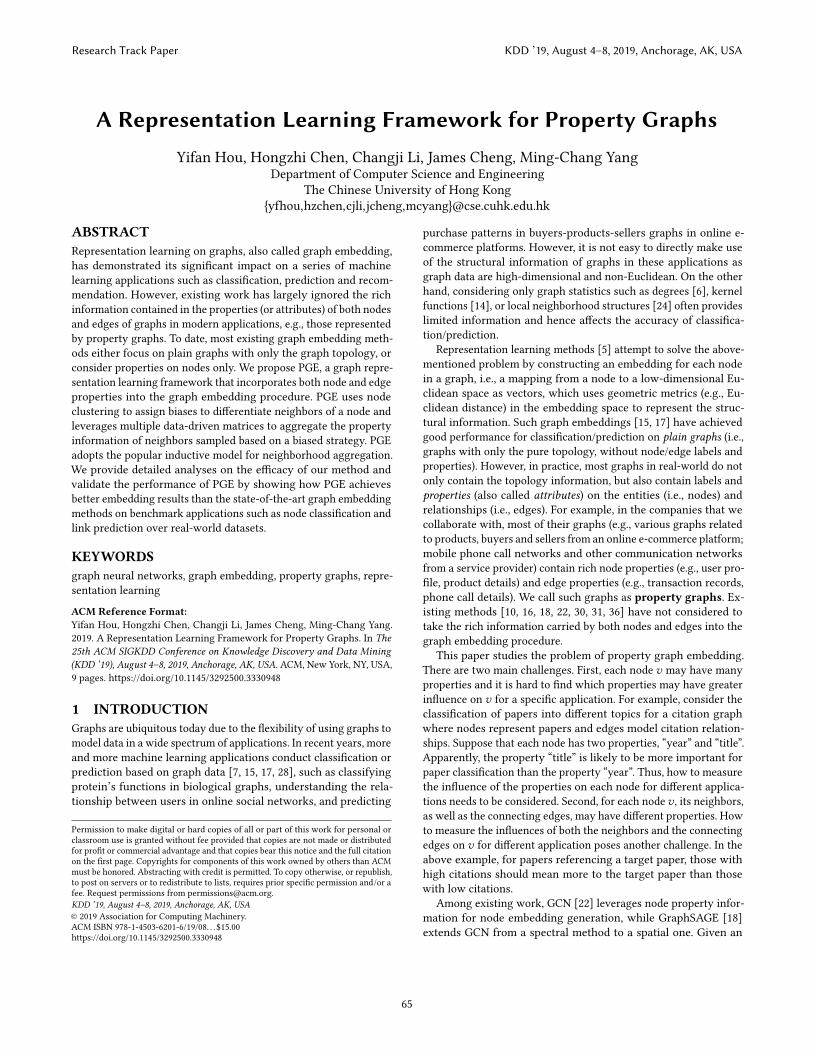
Figure 2: The effects of bias values and cluster number (best viewed as 2D color images)

than that of GraphSAGE. According to the MRR score definition,the correct prediction made by PGE is 1 to 3 positions ahead ofthat made by GraphSAGE. Compared with the improvements madeby PGE for node classification, its improvements for link predic-tion are much more convincing, which can be explained as follows.Differentiating between neighboring nodes may not have a directeffect on predicting a link between two nodes; rather, the use ofedge information by PGE makes a significant difference comparedwith GraphSAGE and the variant of PGE, as the latter two do notuse edge information.

5.3 Parameter Sensitivity TestsIn this set of experiments, we evaluated the effects of the parametersin PGE on its performance.

5.3.1 Effects of the Epoch Number. To test the effects of the numberof training epochs, we compared PGE with GraphSAGE by varyingthe epoch number from 10 to 100. We report the F1-Micro and F1-Macro scores for node classification on the four datasets in Figure 1.The results show that PGE and GraphSAGE have similar trends inF1-Micro and F1-Marco, although PGE always outperforms Graph-SAGE. Note that the training time increases linearly with the epochnumber, but the training time for 100 epochs is also only tens ofseconds (for the small dataset PubMed) to less than 5 minutes (forthe largest dataset Reddit).

5.3.2 Effects of Biases and Cluster Number. We also tested theeffects of different bias values and the number of clusters. We ranPGE for 1,000 times for node classification on PPI, using differentnumber of clusters k and different values of bd (by fixing bs = 1).We used K-Means for Step 1 since it is flexible to change the value

Research Track Paper KDD ’19, August 4–8, 2019, Anchorage, AK, USA

72

k . The number of training epochs was set at 10 for each run of PGE.All the other parameters were set as their default values.

Figure 2 reports the results, where the X -axis shows the numberof clusters k , the Y -axis indicates the logarithmic value (with thebase e) of bd , and the Z -axis is the F1-Micro score (F1-Macro scoreis similar and omitted). The results show that taking a larger bias bd(i.e.,Y > 0) can bring positive influence on the F1-score independentof the cluster number k , and the performance increases as a largerbd is used. When bd is less than 1, i.e., bd < bs , it does not improvethe performance over uniform neighbor sampling (i.e., bd = bs orY = 0). This indicates that selecting a larger number of dissimilarneighbors (as a larger bd means a higher probability of includingdissimilar neighbors into Gs ) helps improve the quality of nodeembedding, which is consistent with our analysis in Section 4.

For the number of clusters k , as the average degree of the PPIgraph is 14.38, when the cluster number is more than 50, the F1-score becomes fluctuating to k (i.e., the shape is like waves inFigure 2). This phenomenon is caused by the limitation of theclustering algorithm, since K-Means is sensitive to noises and alarge k is more likely to be affected by noises. Note that when thecluster number is not large (less than 50), a small bias bd (less than1) may also improve the F1-score, which may be explained by thefact that there are homophily and structural equivalence features inthe graph, while bd < 1 indicates that nodes tend to select similarneighbors to aggregate. In general, however, a large bd and a smallcluster number k (close to the average degree) are more likely toimprove the performance of the neighborhood aggregation method.

6 CONCLUSIONSWe presented a representation learning framework, called PGE, forproperty graph embedding. The key idea of PGE is a three-stepprocedure to leverage both the topology and property informationto obtain a better node embedding result. Our experimental resultsvalidated that, by incorporating the richer information containedin a property graph into the embedding procedure, PGE achievesbetter performance than existing graph embedding methods suchas DeepWalk [30], node2vec [16], GCN [22] and GraphSAGE [18].PGE is a key component in the GNN library of MindSpore — aunified training and inference framework for device, edge, andcloud in Huawei’s full-stack, all-scenario AI portfolio — and has abroad range of applications such as recommendation in Huawei’smobile services, cloud services and 5G IoT applications.

Acknowledgments. We thank the reviewers for their valuablecomments. We also thank Dr. Yu Fan from Huawei for his contribu-tions on the integration of PGE into MindSpore and its applications.This work was supported in part by ITF 6904945 and GRF 14222816.

REFERENCES[1] Nitin Agarwal, Huan Liu, Sudheendra Murthy, Arunabha Sen, and Xufei Wang.

A social identity approach to identify familiar strangers in a social network. InICWSM, 2009.

[2] Amr Ahmed, Nino Shervashidze, Shravan M. Narayanamurthy, Vanja Josifovski,and Alexander J. Smola. Distributed large-scale natural graph factorization. InWWW, pages 37–48, 2013.

[3] Eytan Bakshy, Itamar Rosenn, Cameron Marlow, and Lada A. Adamic. The roleof social networks in information diffusion. InWWW, pages 519–528, 2012.

[4] Mauro Barone and Michele Coscia. Birds of A feather scam together: Trustwor-thiness homophily in A business network. Social Networks, 54.

[5] Yoshua Bengio, Aaron C. Courville, and Pascal Vincent. Representation learning:A review and new perspectives. PAMI, 35:1798–1828, 2013.

[6] Smriti Bhagat, Graham Cormode, and S. Muthukrishnan. Node classification insocial networks. In Social network datanalytics, pages 115–148. 2011.

[7] Michael M. Bronstein, Joan Bruna, Yann LeCun, Arthur Szlam, and Pierre Van-dergheynst. Geometric deep learning: Going beyond euclidean data. IEEE SignalProcessing Magazine, 34.

[8] Shaosheng Cao, Wei Lu, and Qiongkai Xu. Grarep: Learning graph representa-tions with global structural information. In CIKM, pages 891–900, 2015.

[9] Shaosheng Cao, Wei Lu, and Qiongkai Xu. Deep neural networks for learninggraph representations. In AAAI, pages 1145–1152, 2016.

[10] Haochen Chen, Bryan Perozzi, Yifan Hu, and Steven Skiena. HARP: hierarchicalrepresentation learning for networks. In AAAI, pages 2127–2134, 2018.

[11] Jianfei Chen, Jun Zhu, and Le Song. Stochastic training of graph convolutionalnetworks with variance reduction. In ICML, pages 941–949, 2018.

[12] Martin Ester, Hans-Peter Kriegel, Jörg Sander, and Xiaowei Xu. A density-basedalgorithm for discovering clusters in large spatial databases with noise. InSIGKDD, pages 226–231, 1996.

[13] Santo Fortunato. Community detection in graphs. Physics Reports, 486:75–174,2010.

[14] Thomas Gärtner, Tamás Horváth, and Stefan Wrobel. Graph kernels. In Encyclo-pedia of Machine Learning and Data Mining, pages 579–581. 2017.

[15] Palash Goyal and Emilio Ferrara. Graph embedding techniques, applications,and performance: A survey. KBS, 151:78–94, 2018.

[16] Aditya Grover and Jure Leskovec. node2vec: Scalable feature learning for net-works. In SIGKDD, pages 855–864, 2016.

[17] William L. Hamilton, Rex Ying, and Jure Leskovec. Representation learning ongraphs: Methods and applications. IEEE Data Eng. Bull., 40:52–74, 2017.

[18] William L. Hamilton, Zhitao Ying, and Jure Leskovec. Inductive representationlearning on large graphs. In NIPS, pages 1024–1034, 2017.

[19] Keith Henderson, Brian Gallagher, Tina Eliassi-Rad, Hanghang Tong, Sugato Basu,Leman Akoglu, Danai Koutra, Christos Faloutsos, and Lei Li. Rolx: Structuralrole extraction & mining in large graphs. In SIGKDD, pages 1231–1239, 2012.

[20] Geoffrey E. Hinton and Ruslan R. Salakhutdinov. Reducing the dimensionality ofdata with neural networks. Science, 313:504–507, 2006.

[21] Diederik P. Kingma and Jimmy Ba. Adam: A method for stochastic optimization.In ICLR, 2015.

[22] Thomas N. Kipf and Max Welling. Semi-supervised classification with graphconvolutional networks. CoRR, 2016.

[23] Thomas N. Kipf and Max Welling. Variational graph auto-encoders. CoRR, 2016.[24] David Liben-Nowell and Jon M. Kleinberg. The link-prediction problem for social

networks. JASIST, 58:1019–1031, 2007.[25] James MacQueen. Some methods for classification and analysis of multivariate

observations. In Berkeley Symposium on Mathematical Statistics and Probability,volume 1, pages 281–297, 1967.

[26] Tomas Mikolov, Ilya Sutskever, Kai Chen, Gregory S. Corrado, and Jeffrey Dean.Distributed representations of words and phrases and their compositionality. InNIPS, pages 3111–3119, 2013.

[27] Galileo Namata, Ben London, Lise Getoor, Bert Huang, and UMD EDU. Query-driven active surveying for collective classification. In MLG, 2012.

[28] Maximilian Nickel, Kevin Murphy, Volker Tresp, and Evgeniy Gabrilovich. Areview of relational machine learning for knowledge graphs. Proceedings of theIEEE, 104.

[29] Mingdong Ou, Peng Cui, Jian Pei, Ziwei Zhang, and Wenwu Zhu. Asymmetrictransitivity preserving graph embedding. In SIGKDD, pages 1105–1114, 2016.

[30] Bryan Perozzi, Rami Al-Rfou, and Steven Skiena. Deepwalk: Online learning ofsocial representations. In SIGKDD, pages 701–710, 2014.

[31] Bryan Perozzi, Vivek Kulkarni, and Steven Skiena. Walklets: Multiscale graphembeddings for interpretable network classification. CoRR, 2016.

[32] Dragomir R. Radev, Hong Qi, Harris Wu, and Weiguo Fan. Evaluating web-basedquestion answering systems. In LREC, 2002.

[33] Yutaka Sasaki. The truth of the f-measure. Teach Tutor Mater, 1:1–5, 2007.[34] Michael Sejr Schlichtkrull, Thomas N. Kipf, Peter Bloem, Rianne van den Berg,

Ivan Titov, and Max Welling. Modeling relational data with graph convolutionalnetworks. In ESWC, pages 593–607, 2018.

[35] Chris Stark, Bobby-Joe Breitkreutz, Teresa Reguly, Lorrie Boucher, Ashton Bre-itkreutz, and Mike Tyers. Biogrid: A general repository for interaction datasets.Nucleic Acids Research, 34:535–539, 2006.

[36] Daixin Wang, Peng Cui, and Wenwu Zhu. Structural deep network embedding.In SIGKDD, pages 1225–1234, 2016.

[37] Jaewon Yang and Jure Leskovec. Overlapping communities explain core-periphery organization of networks. Proceedings of the IEEE, 102.

Research Track Paper KDD ’19, August 4–8, 2019, Anchorage, AK, USA

73