A RELATIONAL DATABASE MANAGEMENT SYSTEMS APPROACH TO SYSTEM DESIGN by G. Chris Moolman Thesis submitted to the Faculty of the Virginia Polytechnic Institute and State University in partial fulfillment of the requirements for the degree MASTER OF SCIENCE in Systems Engineering APPROVED: Wolter J. Fabrycky, Chairmak Bayan Mae Benjamin S. Blanchard Donald R. Drew February 29, 1992 Blacksburg, Virginia

Welcome message from author
This document is posted to help you gain knowledge. Please leave a comment to let me know what you think about it! Share it to your friends and learn new things together.
Transcript

A RELATIONAL DATABASE MANAGEMENT
SYSTEMS APPROACH TO SYSTEM DESIGN
by
G. Chris Moolman
Thesis submitted to the Faculty of the
Virginia Polytechnic Institute and State University
in partial fulfillment of the requirements for the degree
MASTER OF SCIENCE
in
Systems Engineering
APPROVED:
Wolter J. Fabrycky, Chairmak
Bayan Mae Benjamin S. Blanchard Donald R. Drew
February 29, 1992
Blacksburg, Virginia

5055 V 38S S- IGPR
4 iv

A RELATIONAL DATABASE MANAGEMENT
SYSTEMS APPROACH TO SYSTEM DESIGN
by
G. Chris Moolman
Wolter J. Fabrycky, Chairman
Industrial and Systems Engineering
(ABSTRACT)
Systems are developed to fulfill certain requirements. Several system design configurations usually
can fulfill the technical requirements, but at different equivalent life-cycle costs. The problem is how
to manipulate and evaluate different system configurations so that the required system effectiveness
can be achieved at a minimum equivalent cost. It is also important to have a good definition of all
the major consequences of each design configuration. For each alternative configuration
considered, it is useful to know the number of units to deploy, the inventory and other logistic
requirements, as well as the sensitivity of the system to changes in input variable values.
An intelligent relational database management system is defined to solve the problem described.
Table structures are defined to maintain the required data elements and algorithms are constructed
to manipulate the data to provide the necessary information. The methodology is as follows:
Customer requirements are analyzed in functional terms. Feasible design alternatives are
considered and defined as system design configurations. The reliability characteristics of each
system configuration are determined, initially from a system-level allocation, and later determined
from test and evaluation data. A maintenance analysis is conducted to determine the inventory
requirements (using reliability data) and the other logistic requirements for each design
configuration. A vector of effectiveness measures can be developed for each customer, depending
on objectives, constraints, and risks. These effectiveness measures, consisting of a combination

of performance and cost measures, are used to aid in objectively deciding which alternative is
preferred.
Relationships are defined between the user requirements, the reliability and maintainability of the
system, the number of units deployed, the inventory level, and other logistic characteristics of the
system. A heuristic procedure is developed to interactively manipulate these parameters to obtain
a good solution to the problem with technical performance and cost measures as criteria. Although
it is not guaranteed that the optimal solution will be found, a feasible solution close to the optimal
will be found. Eventually the user will have, at any time, the ability to change the value of any
parameter modelled. The impact on the total system will subsequently be made visible.

TABLE OF CONTENTS
1.0 INTRODUCTION 1.1. Background 1.2 Objective 1.3. Scope 1.4 Approach
eee eee ee eee ee eee eee eee eee ee eee eee eee eee ee rere eee
COMO ee eee rem Oe eee mem am EET EERE TREES HEROS H EATER OEM ESR ED ERH REO RERE EEO HEED
2.0 SYSTEM ANALYSIS 2.1 Customer Requirements 2.2 Product Configuration 2.3 Reliability Assessment 2.4 Maintenance Analysis 2.5 Failure Reporting And Corrective Action System 2.6 Inventory Analysis 2.7 System Effectiveness 2.8 Annual Equivalent Life-Cycle Cost 2.9 Cost Effectiveness 2.10 List of Parameters
3.0 DEFINITION OF MODEL 3.1 Customer Requirements 3.2 Capacity Planning 3.3 System Configuration 3.4 Reliability Assessment
3.5 Maintenance Analysis 3.6 Inventory Analysis
4.0 AHEURISTIC MODEL FOR SYSTEM DESIGN 4.1. Total Number of Failures Per Year
4.2 Operational Availability
4.3 The Heuristic Procedure 4.4 An Example
5.0 SUMMARY, CONCLUSIONS, AND EXTENSIONS 5.1 Summary 5.2 Conclusions 5.3 Future Research
BIBLIOGRAPHY
APPENDIX A: INVENTORY MODELS
APPENDIX B: MANUFACTURING PLANNING AND CONTROL
eee ee ee ee eee eee eee eee eee ee eee eee ree ee eee eT eee eee reese ey
ee ee ee eee eee eee eee ree eee eer eee reer eee ere rere rere ee eee ese res
POM REO e ees OER ee a ROOT MEARE HEE EE HEE HO OOH SE EERE DA REET EEE EDED
SOO ede mew na meee meee trees Dee Eneserareneteeetteretnaenaseseaeseas
CPC eee CVE Veer rea erie ire e rire triers reir
Oe ee eee mera HER OER ROUSE DEEDS EH EO SEES SEREHEDesEEReHbeReEbaY
OPEC E Cer reer eerie rrr rrr restr
Prades eee eee e named ee ne nee E ee HONE O EOE E RES SUHe eS SEK HETeDeOeeEES
oer e errr er eerie rer ricer eerie rier errr iri ters
PPO ede COROT HOOT ERENCE NEC OHE SSE DE DOSEN TOS ROSSA DESE EONS
POO On em eee ene eee OUR TRO EERO OE ERO TOH NOS EEOC OSES EEE ESOEO SORES
POR MEO ODDO T DEDEDE ETE SER SHATTHCEDEEEER SORES OSOEROREEHHEAEE SARE DEES
Saree esesossesmaeesesevessersenesserenes
PPO REE EHO THO REE EEOC SEE DED EF OE NOOR EOE DE HSER SEDER ORO ERODE
CPO e ce Rea eH SOR SOE HOC EASEHE ETH ESESETE RECORD EOE ET EESOeEH
cet ecesneereneerenoenes
POOR O eR EO FORME OE HERES STOO TORS ETE SASSER ETOH ESSAHFES OHSS OFESREODEDSRSEE DE ROEEEETEe
BRO OOOH ERE RT OE FO OE DEERE DROP TORE EFEDEC RST OSH DESH EE REECE R ESSE SE TEE EEEETOCHE SEE
COO e RCE DEER EOE H ESTO ERED SHEETS OT PEN SEHET EE DESSESFCESOSESTORS EEO FED
POOP OO RO Oe RHE DEK ROOT EERE RETESET CERO ES ESES HERES SEES SESEDOSSEDEDSESDESSEDOTERED
PORES S EPO T ROE TET EES ERED SH TOEEAHOESH SOT OEES
Cece ree meee e eee ne RE eee teat eee Ee
Demet a eee ree mame eee Ret eee SEED ee eee
Tamera ccna re eesaeaeenerewarereas emer so nee
OOM MORO R ORO EEE ROO REESE OE AREER TODA R EO EHO HSH HHA ORNS HR OE OTROS AERO EEE EEO SEE ES HEROD EERE DORE OES EES OORT REESE OOO EEO EES OR eee
eee ee ee eee eee eee eee ee eee eee rere
OU ROR ORO Re Oe OREO EOE REE O REET ROMERO HERETO EERE ETOH SEEMED HERETO EE RETO Eee HONORE See REO HOSES UH ON OEE
Peer eh eee RO mat EEO EH ETOH ROE OES H OED EE ETOH OSD DEER EEE S TEER OREO EET Heme eT wate eee EH a te eee
POO O eee eee HOR ERE OTOH EO OEE ESE RETO ETO E DH EO SCHED THERE OHHH EROS ODEO EOE ee EOE EE DEE HEE R HESS E ED
ree ee eee eee err err e ee reer rere rir rer eer errr errr rire riers rer ever ree rerer irri irre irri riers)
POCO Oe RRR O RE Ee OE ARERR E RETO O OE HERE E EH TO REDE OS SESE ROOFER TERETE OEM SE OSES RH ERESEDEE REE DEES HAMEED HOSES
Comet e erate ORO OOH ORR a ORO U FORE DESH SHEED EEO ER OSCE ROS ORHS
Mee neem a cee meee r ete w snes ema eenaeeeeansaeee
Oe ee ee eee ee eee eee rere eee e rise verrr cirri seer etree
CRC e re mee C Oe TERE C OEE OE EEE AHR OE RATE REFER OTHE HER OE REED EDR EOE HEED SHEESH EHEC OEE DEED
Remo s ewe ese necesmate ea reemnvessaeeusennaees
Cee rece mae H emer e aes ee eee eK He Densa Dee EseeD
AO meme Dae e ree m Teo ame eee Ee EHS Dawe DeE HE Eee
emma nara nosnseaseararaserereeuasatesnaveses
Demeester eresaseeseseurveseevenasusDeseae
ORO e Dae e REE Det DRE OED E CEO EE DEERE DA OEE DE
Peer sewers eee Reb SOEs OSES EET DEEDES O EEN EDS
Ome me rererraseseseereseesenareenaseenesoare
Pe mee eres nE teed BowenerBEsasesenererBeuene
Reese wee EHO T RE HEC E HE EESERESEE ESOT ESESSERSEHEUDOE DE SESS DEDEDE DE DADS
Deer rovreverecereanseseeeresssoneeanasaene
Peed erevevaneenoresernsesvesessecrserseenes
Comm nenereosonnesesecenereresenersseevenues
On eee cetenerenseeensecnetacesacasuansonege
CORP CORP ee eT ESET OES UOE HOOT ECA DAT OHSS DEES:
Serer asnereeeeeetearsevseaeesenaeeeonssavets
Ces ecerorereraseseesarseraeenecesenavanere:
SOMO KOH ee Rs eeRaeeEDanDeraeseveeDeseesnenane
PETA H ETRE PA Dees DOPE PEERED EDEsPERH HOE EHE
eee een ese ress eseererrerseesrceamuseeenaeED
PhRoOnhN
=
=2722S550e0000OD
15
15 19
27 41
57

Figure
LIST OF ILLUSTRATIONS
Overview how the proposed model is Structured 0... ee ee ceeeeetereceeseneesneetereeeaeenes 8
Typical Product Structure ...............ccccccccccecesssecesecessseeessnceeseeecesaeessastessessssessessesssessesevereees 23
Example of product Structure OUtDU ..............ccccccceseceseeeseeeeseeeeeecasecsceesecesateasenseecaeeeaeesaees 25
Example of different levels Of repair 2... cescsseceseceseteseceeeeetseeeeateeerersesenetsnceeesesseeseees 42
Product structure of system XYZ (example problem) ..............ceesceeseceeceeceeecesereeeneceers 78
Main elements Of MPC...............:cscccsscsssscecsesceseecsssesaesseeeaeceeeeseceneesersesssesseeseseaseseceseeeeenenees 112

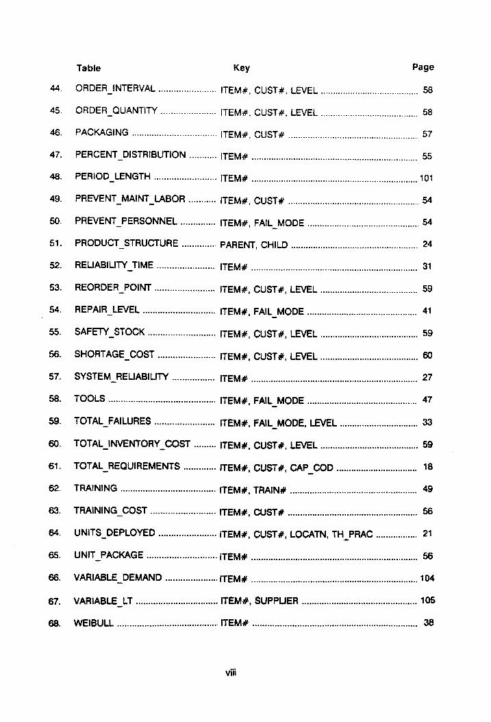
ALPAHBETICAL LIST OF TABLES
The following is a complete list of tables in alphabetical order. The “Key” column indicates the
columns in the tables that uniquely define each row in the table.
Table Key Page
1. ACQUISITION ooceccecccsseecccesseeeee ITEM#, CUSTH ooccccccecccccsssssesccssssneesecssseeesecsssseeeess 50
2. BASE_DATA ....eessesessseescstecsstsesenes ITEM#, FAIL_MODE, FAIL_TIME, TST_TIME ..... 90
3. BILL_OF_ LOCATIONS .................. UNIT oonesseeesssssescssscesssecsesssccssssesessnsessaneceenusesensneteen 42
4. CAPACITY DEPLOYED ................ ITEM#, CUST#, LOCATN, CAP_COD, ............... 22
TH_PRAC
5. CAPACITY DESCRIPTION ........... CODE on eceecccccssesssesssecesscssssccssecessecesseesucssnsessneecsieess 16
6. CENCORED DATA ........ cesses ITEM#, TYPE, REPLACE... sessesecsseccseseseteeee 3g
7. COMMODITY 0... eeceeccccscssstecsssses CODE oooeecsccsessccsssssssecsnsescescsnseesceecnssceecannsseseesseess 26
8. CONSTANT_FAILURES ................. ITEM#, FAIL_MODE .......0.ecccsssesccecssseeccsssereneee 32
9. CONSUMABLES ....00....cecseecesssees ITEM#, CONSUME .......cccccccsesssccsssstscecsenceesecectees S2
10. CORREC_ MAINT LABOR ............ ITEM#, CUSTH onn.ccceccccsseeccsssssececcnsecsecnseeeceneeceseees 53
11. CORRECT PERSONNEL ............. ITEM#, FAIL MODE ..........ccssseccssesccseteccnstesseseesen 53
12. COST PER MILE oo... eceeccseceee ITEM oon.ccccescccsccsececcscccnsceceeecsncecssecsscesaceensesssnesssnes 95
13. CUSTOMER_WORKING HOURS ITEM#, CUSTH# o.......ecscsseecccssssssecscsssesssessneessen 18
14. CUSTOMER WORKING WEEKS ITEM#, CUSTH ou... escsssecsssseeesseesesenesessenss 19
15. DETAIL_REQUIREMENTS ............ ITEM#, CUST#, CAP_COD, LOCATN ............000 7
16. DISTRIBUTION_TYPE ................+. ITEMA oes ceecsecccccsccscssescccvececeneecnsnessssseessssesssaseessunesss 28
17. DOCUMENTATION ..........cecccseee ITEM#, DOCH once cccccsccsssesscceccesseerecsecneneeteceseneneer 48
18. EMQ PRODUCTION ................. ITEM ono eceeecseecssscseseccntecescersecsneesssssssnessseesssesssesss 64

19.
20.
21.
22.
23.
24.
25.
26.
27.
28.
29.
30.
31.
32.
33.
35.
37.
38.
39.
41.
42.
Table Key Page
EOI MULT COST occ ITEM ooeccccescsscccssssscssesesseseesasnseseseseceesnsesssenvanee 98
EOI MULTIPLE_ITEM occ ITEMA oaeecsssssssscssscesesesssssssessecensenssssneseevasnnnseeeen 98
EXPONENTIAL o..ccccscscssssscsseeeeeeveee ITEM#, FAIL MODE oo.o.ccccccccccssccccccssssssssseseneees 34
FACILITIES ...ccccccccceesssssssessseeseece Dn 46
FAILURE MODE .........scsscsccsccscssee (0) 0) 28
GENERAL_DOCUMENTATION ..... DOC#, LEVEL o.cccccsssssssssssssssecssssenssssesesenennnesete 48
GENERAL FACILITIES |... FACIL#, LEVEL o..cccsscessssssesccsssesssssssssssessssessenten 45
GENERAL_PERSONNEL .............. TYPE csccesssssssccssssessessnssnsesssseuunesssnssssensenanasesee 51
GENERAL TOOLS ......sscsssscssssesee TOOL#, LEVEL w.sccssssssssssssessesssssnsssssessssoneeeseeten 47
GENERAL TRAINING 0.0.0... TRAIN#, LEVEL ooscscssscccsssssssssecessssssssessssssesseeeeeee 49
HOLD_FRACTION ....cccscccsssesseseess ITEM#, CUST#, LEVEL o...esscsescssscccssssssseeesensete 60
INV_ITEM MODEL .....cccccessssssoses ITEM#, LEVEL o..ccccccsssssssssssssssssnnnnsesscsssssssneseeee 62
INV_MODEL LIST .....cccccessesessesee 1 62
ITEM_CAPACITY ......cscssssssssescscsee ITEM#, CAP_CODE o..cccscscsssssscsscsssssssesestsnsceeees 20
ITEM_IDENTIFICATION 0.0.00... = 24
ITEM_PERSONNEL ......sccssscsscscese ITEM#, PERS TYPE o..cccsssssscssssssscsssscceseseeseesee 52
ITEM_ PRICE ...cccccccccssccsssssssssneeee ITEM#, SUPPLIER o....sccccccscssssccccecceccsssssseceeeeeeen 25
ITEM_RELIABILITY .....sescsccsccccsen ITEM#, FAIL MODE ........scccccsssssssccscsscceessstscceee 32
MAINTENANCE_CHANNELS ....... TEM#, LEVEL, ACTIVE .0.....-.-ccsssscssssssssseeesesesee 45
MISSION FRACTION .....ccsscsssssese ITEM#, PARENT o.ccssssssccscccsssssscecccsccsstnsssceseeete 19
NONRECUR_COST ......sessssssssssssee ITEM#, LEVEL wcesessssseesssscsccccssssssssnneseccessuensnssetes 44
NORMAL ......sssscscssssssssssssssssnnssseeee ITEM#, FAIL MODE, DISTR .........ccccssssssssceeeeeee 35
OPERATE_CONSUMABLES ......... ITEM#, CUSTH oocecsccsscccssssssesecsssessssnssseeeesecsssee 51
OPERATE_PERSONNEL .............. [TEM#, CUSTH o.cessecssscssssnssssecscsessssnnsssecesessessse 50
ORDER _COST ........sscsssssessseseesssss ITEM#, CUST#, LEVEL .....scscsecsssscssssccsetsssssseesees 60
vii
45.
47.
49.
50.
51.
52.
53.
. 54.
55.
56.
57.
58.
59.
61.
62.
83 g
R
67.
Table Key Page
ORDER_INTERVAL 0... eee ITEM#, CUST#, LEVEL o..ccssscsccsscesecesssssessten 58
ORDER _QUANTITY ...0.....- eee ITEM#, CUST#, LEVEL oo ecceccssssssesssssesseee 58
PACKAGING ........ cee eee ITEM#, CUSTH occ cccccscccecncescetseecentassesees 57
PERCENT_DISTRIBUTION ........... ITEM occccccccccccccccccsseccssssssssesesensssesasennasennenansanansase 55
PERIOD_LENGTH .............0. ITEM occccccscsesescccssssecesessevcccnssssesesesssstssssesssssscesee 101
PREVENT_MAINT LABOR ........... ITEM#, CUSTH# ooo. ececesceeseesessesnessessesseeseeseesnees 54
PREVENT PERSONNEL .............. ITEM#, FAIL_MODE oe ess ecsceessseescseeeeeneee 54
PRODUCT STRUCTURE .............. PARENT, CHILD ooo... ccescsesecesesesesesessesseenes 24
RELIABILITY TIME ............. eee. TEMA ooo ccccccccseescssessssssscssssesscscscssesssusesessessees 31
REORDER_POINT ...............:s2s0 ITEM#, CUST#, LEVEL 0... ecceecsecseecccseceseeseeens 59
REPAIR _LEVEL ..........sssssssssseessseee ITEM#, FAIL_MODE .........sssssssssssssecccesssesecnsssseesess 41
SAFETY _STOCK ..........--seseeeesseee ITEM#, CUST#, LEVEL o......cecccsceesccesseececessseee 59
SHORTAGE _COST .........eeeeeeseeeees ITEM#, CUST#, LEVEL ...0... ec cceceesseeneeee 60
SYSTEM_RELIABILITY ................. ITEM# oo ececcccccsscssccssessecssecsscssecsseessesssesssenetessesseses 27
TOOLS. .....eeeseesesssessesseseeseneeneseesessen ITEM#, FAIL MODE ..........coeccccsesscceeeeecnseeessesees 47
TOTAL_FAILURES ....... ITEM#, FAIL_MODE, LEVEL ......... eee 33
TOTAL_INVENTORY_COST ......... ITEM#, CUST#, LEVEL o.oo ences 59
TOTAL_REQUIREMENTS ............. ITEM#, CUST#, CAP_COD 00... ecsceesesseeesseeeen 18
TRAINING. .......csscscsseessssseessseeesseetees ITEM#, TRAINE ono ccecccccssseeccscsssesccscsseessssssseeesesee 49
TRAINING COST .........cscssccsseeeseees ITEM#, CUSTH# oonsccecccccssseccssseccsseeccnsecenssscesseseesen 56
UNITS_DEPLOYED ................0005: ITEM#, CUST#, LOCATN, TH_PRAC ................. 21
UNIT PACKAGE ..........0seesseeesee TEMA .onccecsscccsssescsessuessscessesssesssesssecsseesssessneesceesnses 56
VARIABLE_DEMAND ...............-000 LS 104
VARIABLE _LT ..ssssccesccstsssessenessseess ITEM#, SUPPLIER ooo... eceeceescecsesssessesseseeeseesseees 105
WEIBULL 20.0... .ccccccccssccesseeseeseeeteeeee: ITEM oon cceececcccccessesssessessscssecsseesntessesosessesstesseesseeas 38
viii

1.0 INTRODUCTION
In this chapter, the background of the problem under consideration is outlined and the output
requirements are defined. The objective and the scope of this research are subsequently defined,
and the approach that is followed, is outlined.
1.1 BACKGROUND
Complex systems are designed and deployed to accomplish one or more operational missions. A
typical example of a complex system is a commercial airliner designed to transport people and
Cargo over a certain distance within a certain time limit. The total life cycle of the system is of
concern. Not only the number of end items deployed, but the entire operating and support
environment is of concern.
During the design and development of complex systems, many alternative concepts and alternative
hardware and software items must be evaluated. Several different design configurations, each with
its own logistic support requirements, may meet the required effectiveness, but at different life-cycle
costs. An end item that requires too much maintenance may be less effective than an alternative
item with a higher reliability. This will probably result from a higher demand on logistic resources
and a resultant lower availability, despite a relatively low first cost. On the other hand, if the item
is too reliable, its first cost may outweigh the savings on the logistic needs. What is the design
configuration that will fulfill the user requirements at the lowest equivalent cost? What are the
logistic needs for this configuration? How does the design team evaluate different design
alternatives?

In order to develop a system that fulfills the requirements at the lowest annual equivalent life-cycle
cost, the following decision variable values must be determined interactively for each possible
design configuration:
1. The number end items to deploy at each location.
2. The inventory level for each item at each location.
3. The reorder point for each item in inventory at each location.
4. The throwaway age for each item.
5. The identification of all test and support equipment, facilities, personnel, documentation,
training, and packaging requirements for each design configuration for each facility at each
level of repair, including the different channels of repair.
It is also important to determine how sensitive the proposed system is (in terms of performance and
cost) to changes in parameters. (The term "parameter’ will be used for all variables and parameters
that will be used in the analysis). This sensitivity is important not only in evaluating different existing
alternatives, but also detecting trends that can serve as a target for the design team. In order to
quantify the sensitivity of the system, a clear relationship must be defined between the number of
end items deployed, the number of spare parts to be carried, and the reliability of the system. The
spare parts that contribute most to the system effectiveness when added to the inventory must be
determined for each deployment situation.
1.2 OBJECTIVE
The objective of this research is to define the structure of a relational database management system
that will enable the user of it to:
1. Evaluate different feasible design configurations of complex systems by manipulating
parameters so that the required system effectiveness can be achieved at a minimum life-
cycle cost.
2. Quantify the logistic support requirements and the total equivalent life-cycle cost for each
possible design configuration, as well as the sensitivity of each configuration to changes
in parameter values.
1.3 SCOPE
This research is undertaken to facilitate decision-making in the evaluation of alternative systems over
the entire life cycle of a system. The proposed model (called the "System Design Evaluation
Model") will be used primarily during the design and development phases, but will continuously be
updated through the production and utilization phases. During the early phases of design, typically
during the concept and preliminary design, different concepts and major components will be
evaluated, using data at a relatively high level. During the detail design phase, the proposed model
will use all the relevant data of all the items in the system that may influence the decision as to
which item is preferable in the context of the system. Low level data are used. Also during the
detail design phase, the number of end items to deploy at each deployment location will be
determined, as well as the different levels of repair, and the facilities and test and support equipment
required at each repair facility at each level of repair. The inventory level for each item in each
repair facility will be determined, as well as when each item must be re-ordered, and in what
quantities.
Maintenance analysis of each design configuration is required to effectively evaluate different design
configurations. During the early design phases, a relatively high level of maintenance analysis is
required to evaluate alternative concepts. However, during the detail design phase, a detailed
maintenance analysis is required. Although the proposed model uses the maintenance analysis data
extensively in evaluating different systems and items, the model is not intended to be a maintenance
analysis package; it merely prescribes what maintenance analysis data are required to effectively
evaluate different systems and items over the intended life cycle of the project.
The proposed model will typically be used in evaluating different complex systems. A system is
considered complex when it is comprised of a high number of component parts, has several
different technology areas involved, and embodies several different performance features. The
systems under consideration are mostly mechanical and/or electrical of nature. Typical examples
include aircraft systems, ground moving equipment, radar systems, etc. Not only the system in its
entirety will be evaluated; each significant item in the system will be evaluated to determine the most
feasible system.
1.4 APPROACH
An intelligent relational database management systems approach is used to accomplish the
objective of this research. The data required to perform the evaluation analysis are identified. The
tables that are defined to maintain the data and the relationships between the different data
elements are defined in Chapter 3. Algorithms are developed in Chapter 4 that will provide the user
of the proposed model with a solution close to the optimal solution. The user is now provided with
4

the ability to change the vaiue of any parameter or data element, as defined in the database
structure, and the resultant effect on the entire system will be made visible. The proposed model
will have the following characteristics:
1. Visibility: The user will have visibility of all the major consequences of each alternative
solution, including the identification of al! the logistic requirements. The level of visibility
depends on the completeness of the maintenance analysis.
2. Consistency: Whenever the value of one parameter changes, the entire model will be
updated (where applicable) and the results will be made visible in real time. For example,
if new test data become available on an item and are entered into the system, the following
will automatically occur without human interference (if the new data differ significantly from
the existing data):
2.1. Item reliability characteristics are updated.
2.2. System availability is updated.
2.3. New order quantities, reorder points, order intervals, and safety stocks are
calculated for each repair facility at each level of repair where that itern is kept in
stock.
2.4. Total available capacity of each location, and of the entire system, are recalculated
and compared with the initial user requirements.
2.5. The new equivalent life-cycle cost is calculated and compared with the existing.
2.6. The net gain (or loss) in cost effectiveness is calculated according to the vector of
effectiveness measures.
Ease of updating: Old data that need to be updated can easily be replaced by entering
new data.
Information retrieval: Any relevant information in any format can be extracted from any
concatenation of any number of relevant tables at any time. This is a tremendously
powerful management tool.
Baseline comparison: Data can be kept for future projects that might have similarities with
the existing project. Continuous improvement in the development of similar systems over
time is likely. The result is a potentially ever-increasing learning curve.
Commonality of data: All users of the proposed model will share the same data. A change
in data will immediately be visible to all users on the network.
Communication: The proposed model will serve as the basis of communication to the
Customer as far as the system is concerned.
Confidence building: The proposed model will increase the confidence with the customer
since the user will have visibility of all major consequences of system related decisions.
10.
Information source: The proposed model will serve as a basic source of information to
develop logistics during the design and development phases.
Data source: The proposed model will serve as a major source of data for material
requirements planning and manufacturing resource planning activities, especially aimed at
the production phase (see Appendix B).
2.0 SYSTEM ANALYSIS
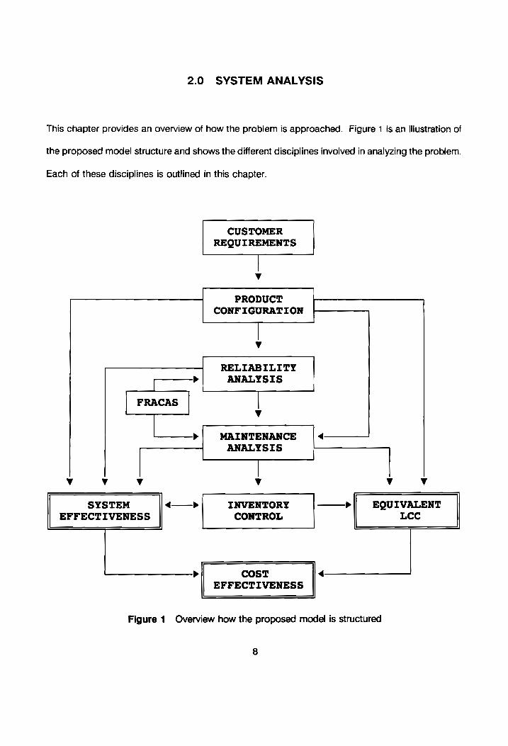
This chapter provides an overview of how the problem is approached. Figure 1 is an illustration of
the proposed model structure and shows the different disciplines involved in analyzing the problem.
Each of these disciplines is outlined in this chapter.
CUSTOMER REQUIREMENTS
v
PRODUCT CONFIGURATION
| v
RELIABILITY > ANALYSIS -—
FRACAS | v
nd MAINTENANCE < a ANALYSIS
Vv Vv Vv v v Vv
SYSTEM <——p INVENTORY > EQUIVALENT EFFECTIVENESS CONTROL LCcc
> Cost < EFFECTIVENESS
Figure 1 Overview how the proposed model is structured

2.1 CUSTOMER REQUIREMENTS
A functional approach is followed in analyzing the customer’s requirements. These requirements
are spelled out in terms of what the customer wishes to accomplish: the number of passengers to
transport, the total amount of ore to mine, the total firepower required, etc.; all as a function of time.
No solutions are offered at this point to fulfill the requirement.
2.2 PRODUCT CONFIGURATION
The product configuration is the most exact definition of each alternative. Although not necessarily
initially defined, this will eventually be the exact definition of each alternative: item numbers, product
structure, specifications, etc. All feasible alternatives are considered for evaluation. Unit capacities
are considered to determine the minimum number of units to deploy.
2.3 RELIABILITY ASSESSMENT
The product configuration, the time period the customer anticipates the equipment to work, and the
way the customer utilizes the system, determine the reliability. The reliability characteristics of each
relevant item in the product structure are determined by test and evaluation. This information is
typically fed to the maintenance analysis to determine the overall inventory requirements for spare
and repair parts.
2.4 MAINTENANCE ANALYSIS
A maintenance analysis is accomplished to determine the logistic requirements of each alternative.
9

The proposed model utilizes maintenance analysis data to evaluate alternative solutions. The
logistic requirements includes the identification of test and support equipment, facilities, manpower,
training, consumables, transportation, and packaging requirements.
2.5 FRACAS
Maintenance analysis is not only accomplished during design and development; it extends over the
entire life cycle of the project. The Failure Reporting And Corrective Action System (FRACAS) is
a process that feeds back data to the developers during the utilization phase of the system. These
data are analyzed to determine if the true reliability of the item deviates from the estimated value.
All relevant logistic support elements are also evaluated.
2.6 INVENTORY ANALYSIS
The demand rate for spare and repair parts are calculated using reliability data, data from the
maintenance analysis, and the system effectiveness requirements. The actual order sizes, reorder
points, order intervals, and safety stocks are calculated for each item at each repair facility for all
the levels of repair.
2.7 SYSTEM EFFECTIVENESS
System effectiveness is an indication of the system's technical capabilities. This includes the system
performance, capacity of the system, reliability, availability, mean time to repair, etc. These
requirements and capabilities are used in evaluating each alternative and the entire system. The
system effectiveness is calculated from the product configuration, its associated reliability
10

characteristics, the maintenance requirements, and the actual inventory of spare and repair parts.
2.8 ANNUAL EQUIVALENT LIFE-CYCLE COST
The annual equivalent life-cycle cost (AELCC) is estimated for each alternative. This is done to aid
in the process of evaluating different alternatives and in determining total costs. The AELCC is
determined from the product configuration, the maintenance requirements, and the actual inventory.
2.9 COST EFFECTIVENESS
The final decision of which alternative to choose will depend on both the system effectiveness and
the equivalent life-cycle cost. The cost effectiveness is the ratio of system effectiveness to the
equivalent life cycle-cost.
2.10 LIST OF PARAMETERS
The following is a list of parameters that will be used in the proposed model. The user can change
values for any of these parameters and the resultant effect on the whole system will be visible:
1. Capacity requirements and constraints.
2. Number of deployment locations.
3. Total amount of hours that the customer expects to work per year.
4. Number of identical items in a higher level item or system.
5. Exact system configuration.
6. The time that each unit is operational, given the total hours required.
11

10.
11.
12.
13.
14.
15.
16.
17.
18.
19.
20.
21.
22.
23.
24.
23.
24.
25.
26.
27.
28.
29.
Unit capacity.
Number or units deployed at each location.
Unit price.
Unit lead time.
Cost Escalating Factor, or inflation rate.
Allocated and actual item reliability values.
item reliability distribution.
Failure data (test times, failure times, etc.).
Time constant used for reliability calculations.
Failure mode and failure rate.
Mean and standard deviation of failure times.
Service level.
Repair level of item.
Number and type of repair levels, and how they are structured.
Distance from repair channel to depot.
Different types of facility requirements and costs.
Different types of tool requirements and costs.
Different types of documentation requirements and costs.
Different types of overhead training requirements and costs.
Disposal requirements and costs.
Different operating personnel requirements and costs.
Different operating consumable requirements and costs.
Different corrective maintenance personnel requirements and costs.
Different preventative maintenance personnel requirements and costs.
Mean corrective maintenance time.
12

30.
31.
32.
33.
34.
35.
36.
37.
38.
39.
40.
41.
42.
43.
45.
47.
49.
50.
51.
52.
53.
54.
Preventative maintenance frequency.
Percentage of spare parts distributed amongst the different levels of repair.
Transportation cost.
Training cost as a variable cost.
Packaging requirements and costs.
Order quantity.
Order interval.
Reorder point.
Safety stock.
Order costs.
Holding costs.
Shortage costs.
Type of inventory model used.
Production rate and length of run for economic manufacturing quantity.
Economic Order Interval items that are acquired together.
Order cost per total order for economic order interval.
Variability of demand.
Variability of lead time.
Variability of lead time and demand.
Mean time between maintenance.
Mean active maintenance time.
Mean and total downtime of the system.
Availability of the system.
Availability of spare parts.
Number of spare parts deployed at each repair site.
13
Some of the parameters in the above list can be calculated from others. However, the user will be
able to override each calculated value and all the relevant tables will be updated accordingly. Also,
some of the parameters listed will have a unique value for each item, eg., reliability. Others may
have a range of values, eg., the number of spare parts to be deployed per level and per customer
for each year. For systems consisting of hundreds or thousands of parts it is therefore not
uncommon to have thousands or even millions of parameter values for all the items. Many of these
parameters have a changing nature: not only price increases and variations in interest rates are of
concern, but numerous others. These include:
1. An alternative supplier has to be found for item X and his promised lead time can not be
considered constant. Extra safety stock must now be carried.
2. New taxes on warehouse property increase the holding cost.
3. The customer wants to add a new intermediate repair facility for every six existing
organizational facilities.
4. The customer wants to carry a greater percentage of parts at the intermediate level for parts
that are repairable at the organizational level.
14
3.0 DEFINITION OF MODEL
The purpose of this chapter is to specify how the model is structured. Because the principles of
relational database management systems are used to achieve the objectives, the different tables in
the model are defined, as well as the relationships among them and the conditions for data
existence and data extraction. Tables are defined as they would actually appear in the database
with the name of the table in bold capital letters just above the table. Between the double lines at
the top of each table are the column definitions. Examples are given to illustrate the types and
format of data relevant for each field.
It is to be noted that all the tables specified in this chapter do not necessarily have to exist in the
database. Tables that contain raw data (data that have not been defined in any other relevant
format) must exist. However, tables that do not contain raw data do not have to exist, since the
required information can be calculated as required from raw data. Whether tables containing non-
raw data exist or not depends mainly on company-specific factors such as the complexity of the
requirements, hardware and software capabilities, frequency of use, configuration management
capabilities and policies, etc. However, for the purposes of illustration, the tables in this chapter are
as extensive as possible without being unnecessarily redundant. (Although the terms "customer"
and "end user" are used synonymoustly, the latter is preferred since each system will be developed
for the user that will use it in its ultimate form.)
3.1 CUSTOMER REQUIREMENTS
As a result of the feasibility study in the conceptual design phase, it is anticipated that the
15

requirements of the end-user will be spelled out in functional terms. Examples include the amount
of iron ore to be transported in a year, the number of passenger miles per year, or the volume of
oil to be pumped per month. The functional objective of the model, as well as the global functional
constraints that are imposed onto the system, are described in the CAPACITY_DESCRIPTION table
and numerically constrained in the DETAIL REQUIREMENTS table. These constraints define the
feasible region in which the eventual system must fall. The objective determines the preferred
solution within the set of feasible solutions.
CAPACITY DESCRIPTION
CODE DESCRIPTION
A Tons of iron ore per year
B Passenger miles per year Cc Barrels of oil per year
A separate table, the END_USER table, keeps track of end user data, such as customer definition
(code, name, location, etc.); customer history (what and when did he buy); and financial status.
The CUSTOMER_ORDERS table links customers and products via an order number. This detail of
the end user is omitted for the purpose of this research.
What is of concern is the actual requirements in functional terms: how much iron ore does the end
user want to mine (and at what locations) per year and for how many years? This type of data is
acquired during the needs analysis phase before design and development actually commences.
The DETAIL_REQUIREMENTS table gives the requirements of each end user per location. The
number of end items is not of concern at this stage. The ITEM# is the end item that is be designed
to fulfill the need. The CUST# is the end user who requires this capability. YR_0, YR_1,..., YR_n
16

are the years he requires the functional capabilities as outlined. YR_0 is the first year that he
requires the capability.
DETAIL REQUIREMENTS
| TTEM# custT# | CAP _cOD| LOCATN YR_O YR_1 YR_n
CBA C342 A L31 7E3 9E3 21E3 CBA C342 G L31 21E6 23E6 49E6 CBA C342 A L19 11E3 12E3 31E3
The ITEM# used in the DETAIL_REQUIREMENTS table typically indicates the end item(s) required
by the customer. Initially, this item does not have to exist; it is the final product to be delivered to
the customer. The CUST# column refers to the customer, or end user, and the CAP_COD is the
capacity code from the CAPACITY DESCRIPTION table to determine the units involved. The
LOCATN column indicates the location where the end user wants to deploy these units. A definition
of these locations can be found in a LOCATION table with columns LOCATION# and
LOCATION _DESCRIPTION (table not shown). The rest of the table represents the years ahead that
contain the functional quantities that are required, corresponding to the type of capacity desired.
As illustrated by the data in the DETAIL_ REQUIREMENTS table, it is possible to have more than one
objective, or constraint, for the same system at any location. (The reason why there is no
distinction made between an objective and a constraint is that these constraints are the end user’s
constraints, and whatever is a constraint for the end user becomes an objective for the company
developing the system.)
The TOTAL_REQUIREMENTS table indicates the total requirements for each end user, regardless
of the location(s) where he anticipates using the system. The total requirements can be the
17

summation of the different detailed requirements, or it can be a constraint that is imposed on the
system as a whole. If there are no constraints on the system other than what is imposed on the
detail level, the TOTAL_REQUIREMENTS table will contain no raw data and can be considered
redundant. Except for the omission of the LOCATN column, all the columns are the same as those
in the DETAIL REQUIREMENTS table.
TOTAL REQUIREMENTS
ITEM# cuSsT# CAP_COD YR_O YR_1 YR n
CBA C342 A 20E3 28E3 65E3 GHI C231 B 54E6 62E6 125E6
Aliso of concern in analyzing the end user’s needs is the amount of hours the end user wants the
equipment to work per week, as well as the number of weeks per year. This information is crucial
in determining the number of units to deploy. The CUSTOMER WORKING_HOURS and the
CUSTOMER_WORKING_WEEKS tables indicate the number of hours the customer wants to work
per week and the number of weeks he wants to work per year for the following n years. For the
remainder of this chapter the columns YR_O ... YR_n will indicate the relevant requirements for the
following n years.
CUSTOMER _ WORKING HOURS
ITEM# CUST# YR_O YR_1 a YR_n
CBA C342 60 60 wee 40 GHI C231 45 50 wee 40
18

CUSTOMER_WORKING_WEEKS
ITEM# cUST# YR_O YR1 wee YR_n
CBA C342 45 50 wee 50 GHI C231 48 48 wee 48
The product of "hours per week" and "weeks per year" is considered the total time per year that the
equipment will be operational. The system will be designed according to this time. The lower level
components of each end item assume the same mission duration each year. This time duration is
therefore passed down the product structure; each lower level component has the same mission
duration as its parent component. If a particular item does not accept the same mission duration
as that of its parent component, that item will be specified in the MISSION FRACTION table as
having a fraction of the time of the parent component. This fraction can be smaller or greater than
one. The PARENT column shows the parent of the item and the FRACTION column shows the
fraction of the parent’s time that will be used as the mission time for that specific item. (The "parent"
principle is discussed in the "Product Configuration" section.)
MISSION_FRACTION
3.2 CAPACITY PLANNING
ITEM# PARENT FRACTION
XDG HJK 0.25
VBN MKL 1.10
Each design configuration is designed to achieve and maintain a certain level of capacity to fulfill
the customer's requirements, as spelled out in the CUSTOMER_REQUIREMENTS table. The
19

number of units to be deployed for the proposed configuration depends on, amongst other factors,
the capacity requirements and the actual unit capacities, including logistics. The unit capacities,
as "designed to" in the top down approach early in design, and the actual unit capacities (bottoms
up) will be maintained in the ITEM CAPACITY table in the DESIGN _TO and ACTUAL columns
respectively. Both the "design to" and the actual capacities are the average operational capacity
per hour when the item is in the "up state" (operational). All downtime activities are excluded in
determining the capacity of each item.
ITEM_CAPACITY
ITEM# CAP_CODE DESIGN TO ACTUAL
CBA A 0.145 0.140
CBA G 13.750 12.210
LMN A 0.125 0.124 When the system is analyzed in the early stages of design and development, the "DESIGN_TO"
values are used to determine the number of units to deploy. However, as more reliable test data
become available, these parameter values are being replaced with the ACTUAL unit capacity. The
original values are kept to evaluate the design process later. The number of units to deploy
depends primarily on the following:
1. Capacity required (defined in the two REQUIREMENTS tables).
2. Actual unit capacity per hour, if available, otherwise the target value (in the ITEM_CAPACITY
table).
3. The time the end user wants to work (defined in the CUSTOMER _WORKING_HOURS and
20

in the CUSTOMER_WORKING WEEKS tables).
Availability factors are considered at a later stage. The theoretical number of units to deploy,
therefore, are the total capacity required, divided by the product of the unit capacity and the time
that the end user wants to work. For each location, the number of units deployed are maintained
in the UNITS DEPLOYED. To obtain the total number of units deployed per location or per
customer (the latter regardless of location), a report can be generated that will calculate the relevant
values. A separate table for the total units deployed would be redundant since it would not contain
any raw data.
UNITS DEPLOYED
ITEM# CUST# LOCATN TH_PRAC YR_O eee YR_n
CBA C342 L31 T 18 eee 72 CBA C342 L31 P 21 eee 85 CBA C342 L19 T 28 eee 107 CBA C342 L19 P 33 eee 126
The column TH_PRAC indicates a theoretical (T) or a practical (P) value. The theoretical values in
the corresponding fields of YR_O through YR_n indicate the number of units to be deployed in order
to fulfill the capacity requirements at an availability of 100%. The reason for using the theoretical
number of units to deploy is to obtain the total amount of effective hours of work needed fulfill the
demand. The total effective hours of work is needed to determine the availability of the system and,
therefore, the actual number of units deployed. The effective hours of work needed are used in the
inventory section and in the heuristic model in Chapter 4.
The capacity that is planned to be deployed, as well as the capacity that is actually being deployed,
21

are maintained in the CAPACITY DEPLOYED table. The TH PRC column indicates whether the
Capacity is based on the theoretical number of units deployed (with availability of 1.0), indicated with
a "T," or the actual number of units deployed with realistic availabilities, indicated with a "P." The
actual number of units deployed are assigned during the detail design phase when the reliabilities
and maintainabilities of the equipment become known with a reasonable amount of certainty and
when a prediction of the relevant availabilities can be made.
CAPACITY DEPLOYED
ITEM# CUST# LOCATN CAP _COD| TH_PRC YR_O eee YRn
CBA C342 L31 A T 7.05E3 cee 20.88E3 CBA C342 L31 A P 6.85E3 eee 19.62E3
CBA C342 L19 A T 10.96E3 eee 31.03E3 CBA C342 L19 A P 10.26E3 eee 30.56E3
As is the case with the UNITS_DEPLOYED table, the totals of the CAPACITY DEPLOYED table can
be obtained by a summation report. It is assumed that the summation of the capacities at the
different locations is the total capacity required. The locations can be assigned such that this
assumption always holds true. However, if this assumption is unacceptable, a separate table will
have to be constructed for the totals: TOTAL_CAPACITY_DEPLOYED. It is strongly recommended
that such a table does not exist and that the locations are selected such that the totals of the
locations equals the total capacity deployed.
3.3 SYSTEM CONFIGURATION
The system configuration is the exact definition of the hardware. It is represented by an item
22

number and gives the lower level components in a product structure, or tree format. The product
structure is a level by level breakdown of the system and of the products comprising the system.
The product structure (sometimes also called the bill of material) is the backbone of the entire
process. All relevant data is linked to the product structure by means of the item number. Different
configurations can be evaluated simply by defining the required configurations either from an
already existing database of items or by adding the required items to the database. The technical
capabilities and the anticipated equivalent life cycle costs and logistic requirements are determined
for each design configuration. A vector of cost effectiveness measures is developed for each
customer against which each configuration will be evaluated. The effectiveness measures depend
on each customer’s objective, constraints and risks. The term "item number" is used for any
component, combination of components, sub-assembly, assembly, or any group of assemblies. The
following tree structure shows the product structure as revealed in the PRODUCT STRUCTURE
table:
cl C2
D1 D2
Figure 2 Typical product structure
23

PRODUCT STRUCTURE
PARENT CHILD QTY PER
A Bl 1 A B2 1
Bl C1 1 Bl C2 1
C2 D1 1
C2 D2 1 The PARENT in the PRODUCT_STRUCTURE table is the item number for which the lower level item
numbers are specified in the CHILD column. The entire product structure of any configuration,
therefore, consists of a logical concatenation of single parent/child relationships. An item (such as
item A above) is therefore not physically built. The advantage of this structure is that any item can
be replaced by another item simply by deleting the original item from its parent and adding the new
item as a lower level component of that parent. The entire system is then updated, provided the
lower level items have been defined.
Another table, TEM_IDENTIFICATION, is used to identify item numbers. Each item is referenced
by only the item number. The item description is only for user interface. The table has the
following structure:
ITEM_IDENTIFICATION
ITEM# DESCRIPTION COMMODITY
A Model XYZ dump truck 236450 Bl Base structure 522200 B2 Container hull 533000
Ci Chassis 212016
ABC Powerpack 142162
Z2Z3 Hinge 800100 ZYX1 Fastener (2.5 x 1/2 inch) 303022
24

When the product structure is printed out, a level-by-level indentation distinguishes the different
levels of components. In the printout the product configuration is taken from the
PRODUCT STRUCTURE table, while the description is from the ITEM_IDENTIFICATION table. Data
which are item related can be grouped together or printed on the same line if space permits. Figure
2 shows a very simple example of a product structure printout:
LEVEL ITEM # DESCRIPTION
0 A Model XYZ 18 wheeler dump truck 1 Bl Base Structure
2 on Chassis 2 C2 Suspension
3 D1 Blade springs
3 D2 McPhersons
1 B2 Cab Figure 3 Example of product structure printout
The ITEM_PRICE table administers the price, lead time, and the cost escalating factor of each item.
The assumption is made (in accordance with Just In Time philosophy) that any number of suppliers
of any item can exist with different prices, but that each item is supplied by only one supplier at only
one price at any one time.
ITEM PRICE
ITEM# SUPPLIER PRICE LEAD TIME| ACTIVE CEF
CBA S432 78640.00 127 N 1.0550 CBA $221 72986.50 142 Y 1.0650 CBA $303 84080.00 113 N 1.0475 XYZ so008 21.99 12 N 1.0450 XYZ $105 19.79 10 YX 1.0525
25
The SUPPLIER column of the ITEM PRICE table is the supplier of the item; PRICE is the current
price of the item; LEAD TIME is the lead time of the item; ACTIVE indicates which supplier is
selected ("Y" is selected, "N" is not selected); and CEF is the cost escalating factor (the factor by
which the price of the item is expected to increase per year). Each item must be selected once and
once only. The lead time is in calendar days and is the amount of time needed to get the item to
the end user, regardless of the path that it follows. An item may be received by the end user
directly from a supplier.
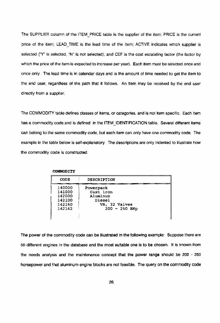
The COMMODITY table defines classes of items, or categories, and is not item specific. Each item
has a commodity code and is defined in the ITEM_IDENTIFICATION table. Several different items
can belong to the same commodity code, but each item can only have one commodity code. The
example in the table below is self-explanatory. The descriptions are only indented to illustrate how
the commodity code is constructed.
COMMODITY
CODE DESCRIPTION
140000 Powerpack 141000 Cast iron 142000 Aluminum
142100 Diesel
142160 V8, 32 Valves
142162 200 - 250 BHp The power of the commodity code can be illustrated in the following example: Suppose there are
50 different engines in the database and the most suitable one is to be chosen. It is known from
the needs analysis and the maintenance concept that the power range should be 200 - 250
horsepower and that aluminum engine blocks are not feasible. The query on the commodity code
26

can now be constructed to include only the feasible engines, and a simulation can be run to
evaluate all these alternatives without human interference. For each alternative, the life-cycle costs
and the logistic requirements are determined and the preferred alternative specified.
3.4 RELIABILITY ASSESSMENT
An initial system level reliability is assigned for the proposed system based upon knowledge of
comparable systems (baseline comparison systems) and a thorough understanding of the customer
need and of available technologies. This initial system level reliability is evaluated during subsequent
stages of design in terms of technical and cost effectiveness measures. Depending on the specific
situation, a whole range of system reliabilities are evaluated in order to determine the best alternative
that will fulfill the need at minimum cost. This analysis process is described in the rest of this
chapter.
System reliability must be broken down into component reliabilities. This is done by means of
reliability allocation (as described by Blanchard and Fabrycky, 1990, chapter 13). The allocation
process is a top down approach that occurs during the early design phases, typically during the
preliminary design phase. The allocated values serve as a baseline against which the actual
reliabilities can be compared.
SYSTEM_RELIABILITY
ITEM# REL_ ALLOCATE REL_ACTUAL
A 0.960 0.9524 Bl 0.989 0.9555
ABC 0.870 0.8450
27

Actual reliabilities become known with more certainty through subsequent phases by means of test
and evaluation. The "actual" reliabilities are then calculated bottoms up to determine whether the
system complies with user requirements or whether it should be (partially) redesigned. The
allocated and measured reliabilities are captured in the SYSTEM RELIABILITY table. To determine
the reliability of a component, it is necessary to know what type of distribution represents the failure
characteristics most accurately. The types are stipulated in the DISTRIBUTION_TYPE table.
DISTRIBUTION_TYPE
ITEM# DESCRIPTION
ABC EXPONENTIAL
DD1 LOGNORMAL
CDFB WEIBULL
794D CENSORED DATA Items are subject to different types of failures. A separate table defines the different failure
modes. The failure modes are constructed in the same way as the commodity codes in that the
failure modes are generic and therefore not dependent on an item. Each item can have several
failure modes. The FAILURE_MODES table maintains the different failure mode definitions.
FAILURE_MODES
MODE DESCRIPTION
1015 SHEER 3550 OVERHEAT
4400 WEAR OUT
1650 LEAK
7777 [Bottoms-up summation] 28

Some failures can be grouped together, or all failures of an item can be treated alike, depending
on what is required. However, the more elaborate the data requirements, the better the feedback
to redesign. Also, the physical size of the failure mode identifier (MODE in the FAILURE _MODE
table) does not have to be four characters; it can be any size.
The failure modes are constructed in such a way that each failure mode has a unique task type.
A certain failure mode (or one or more characters within the failure mode) might indicate that the
specific failure mode will be repaired by adjustment without replacement; again, regardless of the
item number. The failure mode can therefore also be constructed such that a failure mode starting
with any digit other than 9 necessarily implies repair by replacement. A 9... failure mode, therefore,
does not demand a replacement. The failure modes are used extensively in the reliability model to
determine the failure rate of an item.
A distinction is made between the total failure rate of an item and its inherent failure rate: An
inherent failure rate is defined as a failure rate unique to an item where the item is treated as a
complete entity in itself regarding that failure. For the purposes of this research, inherent failure rate
does not necessarily mean "true" failure rate. If the failure demands a replacement, the entire item
will be replaced, regardless of the level of complexity. For example, an engine might seize. The
entire engine needs to be replaced instead of just the pistons, bearings, or the engine block.
Therefore, inventory has to be carried for items other than just the lowest level components. An
inherent failure rate is, therefore, a characteristic inherent to an item, while the total failure rate is
the total failure rate of an item, calculated as the summation of the following:
1. The item’s inherent failure rates.
2. The failure rates of the item’s lower level components.
29

An item’s total failure rate due to the summation of the failure rates of its lower level components
is distinguished from its inherent failure rates by the way that the failure modes are structured.
Failure mode 7777 typically denotes the summation of failure rates of lower level components, while
the other failure modes can be failure specific.
Failure data become available during test and evaluation procedures. These data are then captured
in the BASE_DATA table.
BASE_DATA
ITEM# FAIL MODE|FAIL TIME|TST TIME| DATE ACTIVE
ABC 1015 1274 1274 2/04/91 Y ABC 1015 1406 1406 2/04/91 Y
ABC 3550 1051 1051 6/07/90 N ABC 4400 xe RR 3207 7/08/89 Y
The column FAIL_TIME is the length of time that the item lasted before it failed. The TST TIME
column is the total time that the item was tested. If the iter did not fail during the test (test aborted
before failure), then the total time that the item was tested is noted in the TST_TIME column and
the FAIL_TIME is cleared and flagged. Different conditions (other than normal working conditions)
can be facilitated by means of the failure mode. The DATE column is the date when the tests were
accomplished. The user can now choose the data that he prefers by specifying certain dates that
will exclude undesired failure data. The dates also provide visibility in the reliability growth of the
item over time. The ACTIVE column is a means to select data with or without specifying certain
dates.
30
The data in the BASE DATA table together with the type of distribution used from the
DISTRIBUTION_ TYPE table determine the reliability and failure rate characteristics. Each distribution
type has a separate table to maintain the relevant parameter values as calculated from the data in
the BASE_DATA table. The actual reliability values can be calculated directly from the BASE_ DATA
table, but due to the frequent use of this type of information, separate tables are constructed for
each of the distributions. This means that whenever the data in the BASE DATA table change or
when the selection criteria change, the relevant distribution tables must be updated.
Since the system is a repairable system, the reliability of the system degrades as the system is
being used, but increases as the system is repaired. Because of this fluctuation in the reliability, a
time period must be negotiated with the end user for whom the system is being designed to
determine a desired reliability. This only holds if the system is employed “indefinitely” (i.e., used as
long as it is economically feasible). Examples of such systems include ground excavation and
transportation. If the system is used to fulfill multiple, discrete missions during which no repair is
possible, the anticipated mission durations must be specified. The CUSTOMER_WORKING_WEEKS
and the CUSTOMER_WORKING_HOURS tables will then be multiples of these durations. Examples
of such systems include spacecraft and certain remote controlled equipment.
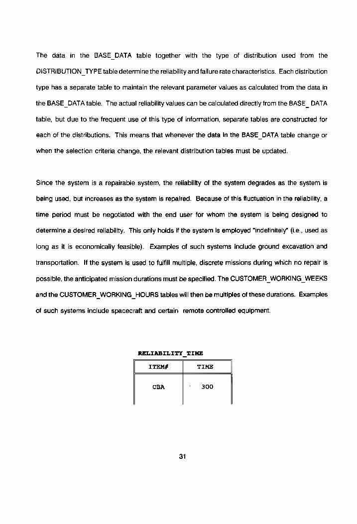
RELIABILITY TIME
ITEM# TIME
CBA ‘300
31

The RELIABILITY_TIME table specifies (in the TIME column) the time duration in hours for which the
system is designed. All the lower level components are treated according to this time and the
MISSION FRACTION table.
The reliability of each item is calculated based on the time in the RELIABILITY_TIME table and on
the parameters that define the specific distribution that represents the failure characteristics. The
procedure to estimate these parameters is discussed in the rest of this section. The reliability values
of each item and each relevant failure mode are defined in the ITEM_RELIABILITY table.
ITEM _RELIABILITY
ITEM# FAIL MODE RELIABILITY
ABC 1015 0.9950
ABC 3550 0.9320 ABC 7777 0.9250
XYZ 1659 0.9650
XYZ 3550 0.9875 A distinction is made between failures that occur independent of the time that the item is utilized,
and failures that are dependent on the time that they are utilized. Time-independent failure rates
are maintained in the CONSTANT _FAILURES table. The column FAIL_RATE is the failure rate of
the item for a specific failure mode. The units are failures per operating hour.
CONSTANT FAILURES
ITEM# FAIL MODE FAIL RATE
ABC 1015 0.0050 ABC 3550 0.0704 ABC 7777 0.0780 XYZ 1659 0.0356
32

The total number of failures that are anticipated to occur during each year (as a function of the total
theoretical number of units deployed per location) are maintained in the TOTAL FAILURES table.
Time-independent failures are calculated as the failure rate of the item in the CONSTANT_ FAILURES
table multiplied by the total time that the end-user expects to work. The latter is the product of the
times for each year inthe CUSTOMER _WORKING_HOURS and the CUSTOMER_WORKING WEEKS
tables. For time-dependent failures, the time that the system is operational per year is used as the
time constant in calculating the failure rate. This is explained in subsequent sections. The columns
YR_0, YR_1, ..., YR_n indicate the total failure rates in the first, second, and so on, until the n'” year.
TOTAL FAILURES
ITEM# |FAIL MODE| LOCATN YR_O YR_1 wee YR n
ABC 1015 LO3 12 15 wee 31 CFG 3569 L21 45 57 eee 76
These failures act as the primary demand for spare and repair parts. The TOTAL_FAILURES table
is, therefore, a very important table as far as inventory control is concerned. The failure modes are
all inherent failure modes that demand a replacement upon failure. The FAIL_MODE column should
therefore include all failure modes except 7777 and those starting with a 9... . Inventory is,
therefore, kept for all the items listed in the TOTAL_FAILURES table, although not in those
quantities.
The primary sources of information for the remainder of Section 3.4 are the following: Dhillon
(1983), Dhillon and Singh (1981), Lewis (1987), and O’Connor (1985).
33
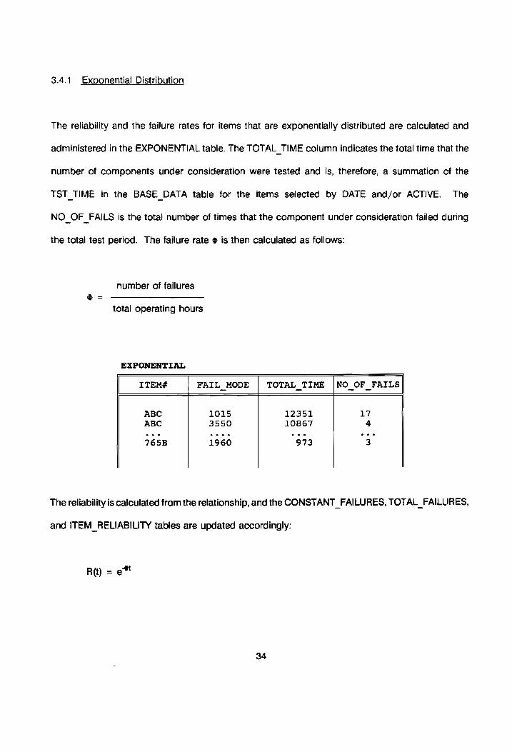
3.4.1. Exponential Distribution
The reliability and the failure rates for items that are exponentially distributed are calculated and
administered in the EXPONENTIAL table. The TOTAL_TIME column indicates the total time that the
number of components under consideration were tested and is, therefore, a summation of the
TST_TIME in the BASE DATA table for the items selected by DATE and/or ACTIVE. The
NO_OF FAILS is the total number of times that the component under consideration failed during
the total test period. The failure rate © is then calculated as follows:
number of failures
total operating hours
EXPONENTIAL
ITEM# FAIL MODE | TOTAL TIME |NO OF FAILS
ABC 1015 12351 17 ABC 3550 10867 4
765B 1960 973 3 The reliability is calculated from the relationship, and the CONSTANT_FAILURES, TOTAL_FAILURES,
and ITEM_RELIABILITY tables are updated accordingly:
R(t) = e*
34
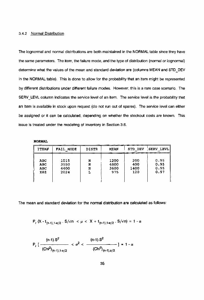
3.4.2. Normal Distribution
The lognormal and normal distributions are both maintained in the NORMAL table since they have
the same parameters. The item, the failure mode, and the type of distribution (normal or lognormal)
determine what the values of the mean and standard deviation are (columns MEAN and STD_DEV
in the NORMAL table). This is done to allow for the probability that an item might be represented
by different distributions under different failure modes. However, this is a rare case scenario. The
SERV_LEVL column indicates the service level of an item. The service level is the probability that
an item is available in stock upon request (do not run out of spares). The service level can either
be assigned or it can be calculated, depending on whether the stockout costs are known. This
issue is treated under the modeling of inventory in Section 3.6.
NORMAL
ITEM# FAIL MODE DISTR MEAN STD_DEV |SERV_LEVL
ABC 1015 N 1200 200 0.95 ABC 3550 N 4800 400 0.95 ABC 4400 N 3600 1400 0.95 X8Z 2024 L 975 120 0.97
The mean and standard deviation for the normal distribution are calculated as follows:
P,X - tert) saj2:S/V0 <u < Xt tiny yee S/¥n) = 1-a
(n-1).$? Pl
(Chi?) 9.1) 1-0/2 <o <
(n-1).S2
(Chi?) 9-1),0/2
35
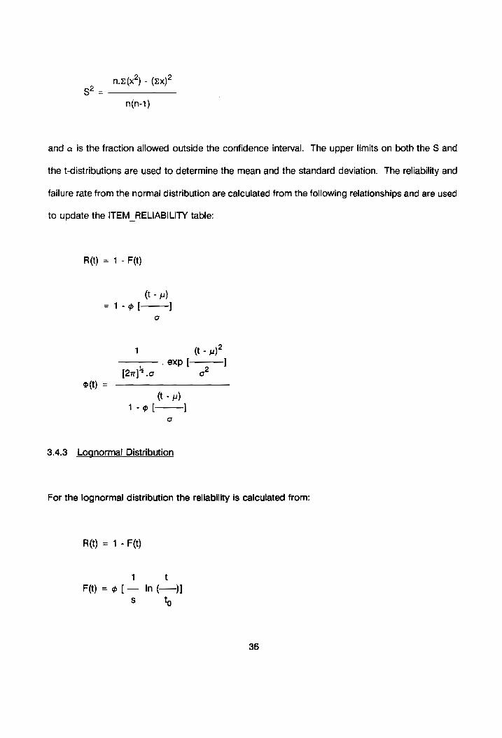
, n.z=(x°) - (zx)? st = ——___—
n(n-1)
and a is the fraction allowed outside the confidence interval. The upper limits on both the S and
the t-distributions are used to determine the mean and the standard deviation. The reliability and
failure rate from the normal distribution are calculated from the following relationships and are used
to update the ITEM RELIABILITY table:
Rit) = 1 - F(t)
(t - y) =1-9| ]
1 (t - 4)? —— . exp [ ]
[21]? .o a” a(t) =
(t - ») 1-9 [ ]
3.4.3. Lognormal Distribution
For the lognormal distribution the reliability is calculated from:
R(t) = 1 - F(t)
1 t
Ft) = @[— In(—) $ Ke
36

2 and the MTBF, y, and the variance, o“, are given by:
57
MTBF = pu = ty exp (—) 2
om = to” exp (s”) * [exp (s*) - 1]
t, is calculated from the relationship (the geometric mean):
to = (t * t*)?
where the values t’ and t” are chosen as the lower and upper limits of the data between which a
large percentage of all data points fall. Since the user has the ability to select the values to be
included from the BASE_DATA table by means of the DATE and ACTIVITY columns, the model
assumes that t is the lowest value and t* is the highest value and that 95% of all data points are
included in this range. However, the user is prompted to justify these assumptions or alternatively
to adjust them. The value of n then satisfies the following relationships:
From the probability anticipated that all the data points are included in the interval t and t™ the
value of Z can be obtained from normal distribution tables. The value of s is then obtained from:
37
s = (—) * In (n)
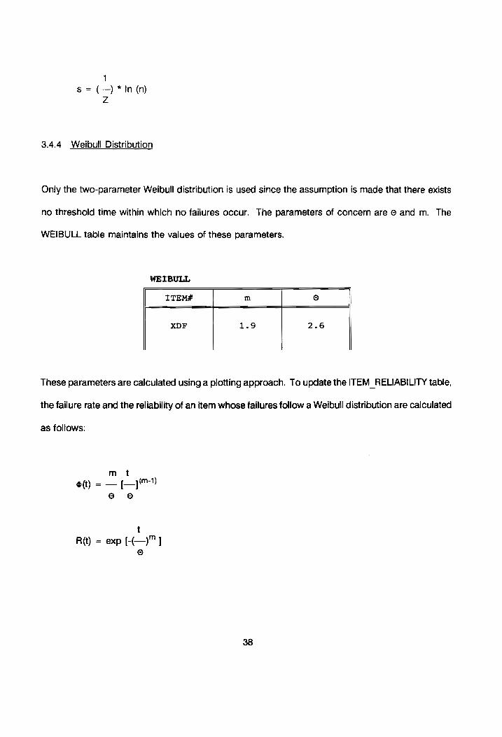
3.4.4 Weibull Distribution
Only the two-parameter Weibull distribution is used since the assumption is made that there exists
no threshold time within which no failures occur. The parameters of concern are © and m. The
WEIBULL table maintains the values of these parameters.
WEIBULL
ITEM# m ©
XxDF 1.9 2.6
These parameters are calculated using a plotting approach. To update the ITEM RELIABILITY table,
the failure rate and the reliability of an item whose failures follow a Weibull distribution are calculated
as follows:
m t
et) = —T™ © oO
t
R(t) = exp [-(—)™] 0
38
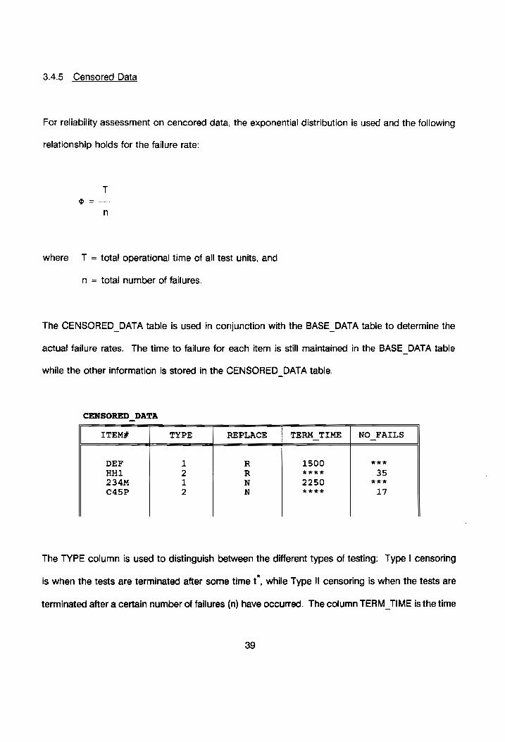
3.4.5 Censored Data
For reliability assessment on cencored data, the exponential distribution is used and the following
relationship holds for the failure rate:
T
b= — n
where T = total operational time of all test units, and
n = total number of failures.
The CENSORED_DATA table is used in conjunction with the BASE_DATA table to determine the
actual failure rates. The time to failure for each item is still maintained in the BASE_DATA table
while the other information is stored in the CENSORED_DATA table.
CENSORED DATA
ITEM# TYPE REPLACE TERM_TIME NO_ FAILS
DEF 1 R 1500 eeK HH1 2 R exKK 35 234M 1 N 2250 aK c45P 2 N ake 17
The TYPE column is used to distinguish between the different types of testing: Type | censoring
is when the tests are terminated after some time t., while Type Il censoring is when the tests are
terminated after a certain number of failures (n) have occurred. The column TERM_TIME is the time
39

(tt) when the tests are terminated for Type | testing. Only Type | testing can have a termination
time, whether the failed components are replaced or not. This column, therefore, is left blank in the
case of Type Il testing. The NO_FAILS column determines the number of failures after which the
tests on a Type II testing should be terminated. Likewise, this field is left blank for Type | testing.
Care should be taken in the selection of the correct data in the BASE DATA table. Only the
applicable test data should be selected by either the DATE or the ACTIVE column or by both. In
the calculation of the failure rate, the value of T assumes the following values under the conditions
stated:
Type |: Non-replacement
n *
T= = t + (N-njt
where t; is the time at failure for component i. N units are tested and n failed. Therefore, N-n units
operated the full time.
Type Il_: Non-replacement
t, + (N-n)t, + It
[Mo
The number of items that failed in areas other than those tested for (in the non-replacement case)
are subtracted from the total number of failures.

Type | : Replacement gives
T= Nt
Type Il : Replacement
3.5 MAINTENANCE ANALYSIS
The level at which an item with a specific failure rate can be repaired is indicated in the table
REPAIR_LEVEL. Any number of levels can exist, as long as the level has been defined. No
distinction is made as to which specific repair facilities are of concern; only the level is of concern.
REPAIR LEVEL
ITEM# FAIL MODE LEVEL
SDF 5604 oO KLM 1015 D OPQ 2250 I
The different levels of repair and the actual repair facilities can now be constructed in similar fashion
as the product structure, as is illustrated in Figure 4. The blocks L11 to L23 in Figure 4 indicate the
different locations where the end items will be deployed. Each deployment location has its own
organizational level of repair, denoted by O11 to 023. Intermediate levels of repair (101 and 102) are
provided for groups of organizational repair facilities. A depot repair facility (D01) is similarly
41
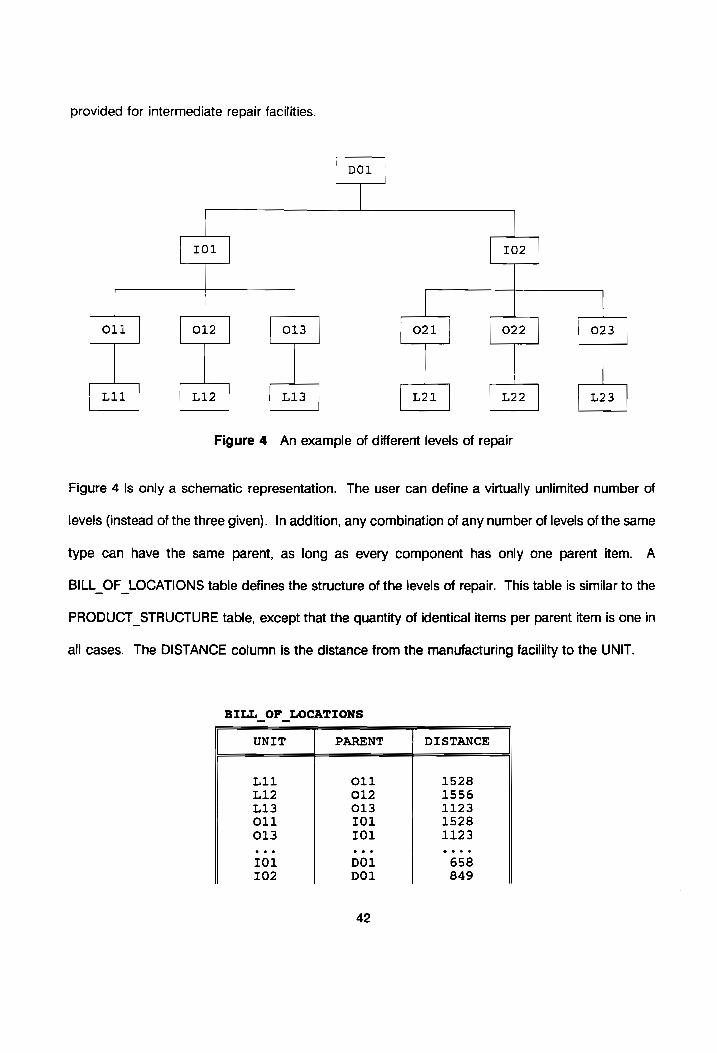
provided for intermediate repair facilities.
DOL
I01 I02
oll 012 013 021 022 023
Lil L12 L13 L21 L22 L23
Figure 4 An example of different levels of repair
Figure 4 is only a schematic representation. The user can define a virtually unlimited number of
levels (instead of the three given). In addition, any combination of any number of levels of the same
type can have the same parent, as long as every component has only one parent item. A
BILL_OF_LOCATIONS table defines the structure of the levels of repair. This table is similar to the
PRODUCT STRUCTURE table, except that the quantity of identical items per parent item is one in
all cases. The DISTANCE column is the distance from the manufacturing facililty to the UNIT.
BILL_OF_ LOCATIONS
a UNIT PARENT DISTANCE
Lil O11 1528 L12 012 1556 L13 013 1123 011 I01 1528 013 I01 1123
I01l Dol 658 I02 pol 849
42
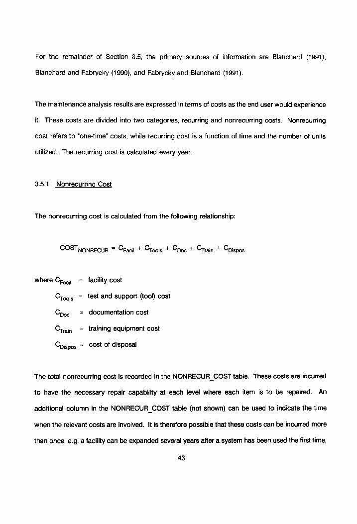
For the remainder of Section 3.5, the primary sources of information are Blanchard (1991),
Blanchard and Fabrycky (1990), and Fabrycky and Blanchard (1991).
The maintenance analysis results are expressed in terms of costs as the end user would experience
it. These costs are divided into two categories, recurring and nonrecurring costs. Nonrecurring
cost refers to “one-time” costs, while recurring cost is a function of time and the number of units
utilized. The recurring cost is calculated every year.
3.5.1. Nonrecurring Cost
The nonrecurring cost is calculated from the following relationship:
COST oNRECUR = Craci + Crools + Coe + Ctrain + Cbispos
where Ce.., = facility cost
Crools = test and support (tool) cost
Coee documentation cost
Crain
Chispos = Cost of disposal
training equipment cost
The total nonrecurring cost is recorded in the NONRECUR_COST table. These costs are incurred
to have the necessary repair capability at each level where each item is to be repaired. An
additional column in the NONRECUR_COST table (not shown) can be used to indicate the time
when the relevant costs are involved. It is therefore possible that these costs can be incurred more
than once, e.g. a facility can be expanded several years after a system has been used the first time,
43

or new repair documentation may be required because of end items that were upgraded to a new
configuration.
NONRECUR_COST
ITEM# LEVEL FACILT TOOLS DOCUMNT TRAINNG DISPOS
ABC I03 120000 35000 16000 12000 25000
ABC D 45000 35000 16000 8000 15000
The LEVEL column in the NONRECUR_COST table is the maintenance level of concern. The
maintenance levels are operational (O), intermediate (I), and depot(D). These distinctions are made
because the logistic requirements usually differ from level to level and even within levels. Therefore,
the different levels can be further subdivided. Level 021 typically indicates a specific (probably
geographically bound) organizational maintenance and repair facility. In such a way different levels
can be evaluated, as well as different repair facilities within levels.
The type of maintenance level, and the items that will utilize these facilities (typically end items), are
maintained in the MAINTENANCE LEVELS table. The item numbers in this case typically are end
items (i.e., the final product without support). The LEVEL column indicates the specific level where
the maintenance is accomplished. The COST column indicates the cost associated with the specific
level of maintenance for the item under consideration. The COST column shows the summation
of all the nonrecurring costs for the item for that level of repair. In the ACTIVE column, each level
of repair can be activated or deactivated for consideration.

MAINTENANCE LEVELS
ITEM# LEVEL COST ACTIVE
ABC D 1265338 XY
ABC I01 376751 Y ABC I03 567089 N
ABC 021 236055 XY The GENERAL FACILITY table indicates the type of facilities that are available, or can be made
available, with the associated costs. These facilities are not related to item numbers in this table
This table houses a list of all relevant facilities. Alternative facilities can be selected in the
FACILITIES table, which is item related. The FACIL# column in the GENERAL FACILITY table is
the unique identifier of each facility. The FACIL# is exactly the same as the ITEM# and, therefore,
must also be identified in the ITEM_IDENTIFICATION table. The reason it is not called the ITEM#
is that in the FACILITIES table the facilities are logically associated with items. The facilities that are
needed to maintain and repair items are linked to those items. The reason the FACIL# and the
ITEM# must be of the same type is that item descriptions are only maintained in the
ITEM_IDENTIFICATION table; but more importantly, product structures must be constructed from
the same source. Each facility is also associated with a commodity code, a requirement from the
ITEM_IDENTIFICATION table. This association allows the user to make a printout of all the facilities
under consideration, or to treat those as a separate group of facilities.
GENERAL FACILITIES
FACIL# | LEVEL ** DESCRIPTION ** COST COMMON
F541 012 EMPTY WORKSHOP (SCRATCH) 75000 N F446 13 EXIST WORKSHOP (EXPAND) 52000 Y F340 D EXIST WORKSHOP (EXPAND) 15000 Y D870 14 UL.SON CRACK TESTING 23000 N W368 D DEGREASE WASH BATH 17000 N G179 07 CALIBRATION SHOP 85000 Y
45
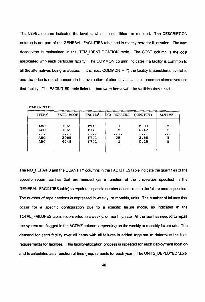
The LEVEL column indicates the level at which the facilities are required. The DESCRIPTION
column is not part of the GENERAL FACILITIES table and is merely here for illustration. The item
description is maintained in the ITEM_IDENTIFICATION table. The COST column is the cost
associated with each particular facility. The COMMON column indicates if a facility is common to
all the alternatives being evaluated. If it is, (i.e., COMMON = Y) the facility is considered available
and the price is not of concern in the evaluation of alternatives since all common alternatives use
that facility. The FACILITIES table links the hardware items with the facilities they need.
FACILITIES
ITEM# FAIL MODE FACIL# NO_ REPAIRS; QUANTITY ACTIVE
ABC 3065 F741 1 0.33 N
ABC 3065 F741 2 0.42 Y
ABC 3065 F741 25 3.65 N
ABC 4048 F741 1 0.15 N The NO_REPAIRS and the QUANTITY columns in the FACILITIES table indicate the quantities of the
specific repair facilities that are needed (as a function of the unit-values specified in the
GENERAL FACILITIES table) to repair the specific number of units due to the failure mode specified.
The number of repair actions is expressed in weekly, or monthly, units. The number of failures that
occur for a specific configuration due to a specific failure mode, as indicated in the
TOTAL_FAILURES table, is converted to a weekly, or monthly, rate. All the facilities needed to repair
the system are flagged in the ACTIVE column, depending on the weekly or monthly failure rate. The
demand for each facility over all items with all failures is added together to determine the total
requirements for facilities. This facility-allocation process is repeated for each deployment location
and is calculated as a function of time (requirements for each year). The UNITS DEPLOYED table,
46

the REPAIR LEVEL table, the BILL_OF LOCATIONS table, and the PERCENTAGE DISTRIBUTION
table (to be discussed later) are all used to allocate the facility requirements to each repair facility
at each level of repair. This allocation process is discussed in chapter 4. The specific level of repair
and the demand per year are not shown in the FACILITIES table.
The TOOLS, DOCUMNT, and TRAINNG columns in the FIXED_COST table have basically the same
format as the FACILT column. The TOOLS column is the accumulation of costs of all test and
support equipment. The GENERAL TOOLS table is a listing of all tools that are available and is
equivalent to the GENERAL FACILITIES table. The same types of tables exist for the documentation
and training as for tools and facilities. In all cases, the description is not part of the tables
themselves. It is part of the ITEM_IDENTIFICATION table and is shown for clarity.
GENERAL TOOLS
TOOL# LEVEL ** DESCRIPTION ** COsT COMMON
T354 o12 HYDRAULIC TEST BENCH 128500 N T337 I3 SPECIAL HOIST 52000 Y G650 D TRANSPORTATION TRUCK 87250 N
TOOLS
ITEM# FAIL MODE TOOL# NO_REPAIRS| QUANTITY ACTIVE
ABC 3065 T337 1 1.25 N ABC 3065 T337 2 2.50 b 4
ABC 3065 T337 25 30.00 N ABC 4048 T337 1 0.75 N
47

The TOOLS table (containing the requirements for test and support equipment) is constructed
similar to the FACILITIES table. The test and support equipment is allocated to the different repair
facilities in the same way as the facilities. As is the case with the FACILITIES, the test and support
equipment requirements are given per year for each repair facility at each level of repair. This detail
is not shown in the TOOLS table. The structure of the TOOLS table enables the user to determine
the tool requirements for a specific failure mode at each repair facility, or for a given item and a
failure mode, or for a failure mode (with or without the item specified) that involves some form of
failure. For example, the user can now query the system for all the tools required to repair a
cylinder head of an engine if the valves have burned.
The GENERAL DOCUMENTATION and the DOCUMENTATION tables, as well as the
GENERAL _TRAINING and TRAINING tables, are constructed in the same way as the tables for the
test and support equipment and facility requirements.
GENERAL DOCUMENTATION
DOC# LEVEL **x DESCRIPTION ** cost COMMON
D123 D ILLUSTRATED PARTS CATALOG 357750 N
D668 I2 WORKSHOP REPAIR MANUAL 256800 N D993 023 PREVENT LUBR INSTRUCTIONS 65350 N
DOCUMENTATION
ITEM# FAIL_MODE DOC# NO REPAIRS| QUANTITY ACTIVE
ABC 3065 D123 1 0.35 N
ABC 3065 D123 2 0.70 Y
ABC 3065 D123 25 15.50 N
ABC 3065 D987 1 0.75 N

GENERAL TRAINING
TRAIN# LEVEL ** DESCRIPTION ** COST COMMON
TRO3 D FLIGHT SIMULATOR 2456750 N
TR68 I5 TEST BENCH (ELECTRIC) 45600 N TRG3 023 WIRING SIMULATION BENCH 35250 N
TRAINING
ITEM# FAIL MODE TRAIN# NO_REPAIRS| QUANTITY ACTIVE
ABC 3065 TR68 1 0.15 N
ABC 3065 TR68 2 0.25 XY
ABC 3065 TR68 25 3.10 N ABC 3065 TRO3 1 0.75 N
3.5.2 Recurring Cost
The recurring cost (as a function of time and the number of units deployed per year) is determined
from the following relationship:
COSTrecur = CUnit + Coper + Ciny + CLabr + Ctrans + Crain + Crack
where Cy, = Unit cost
Coper = Cost to operate the equipment
oO
2 ! Inventory cost
Ci abr = Labor cost of corrective and preventive maintenance
Crans = Transportation cost
Training cost ~ 2.
3
|
Packaging, preservation, and handling cost QO
U0 ~ ° xn
\
49

Each of these costs has a table to maintain the different annual costs involved for the next n years:
The unit cost is the cost of one unit of the end item. This includes development and production
costs, but excludes support cost. For each year, this cost is the unit cost in the ITEM_PRICE table,
multiplied by the product of the cost escalating factor (CEF) in the ITEM_PRICE table and the year
that is of concern. These costs are maintained in the ACQUISITION table.
ACQUISITION
ITEM# cusT# YR_O wee YR n
CBA C342 313757.00 a 7453698.00
The cost to operate the system is calculated as the sum of the personnel cost and the consumable
cost, for example, gas. The OPERATE PERSONNEL and OPERATE_CONSUMABLES tables
indicate these respective costs. The total operations cost then is:
Coper = Coes + Coons
where C,,,, = personnel cost to operate one unit for the entire mission duration
Coons = Cost of consumables (gas, etc) to operate one unit for the entire mission
OPERATE PERSONNEL
ITEM# cUST# YR_O a YR_n
CBA C342 1265045 wee 7689345
50

OPERATE _CONSUMABLES
ITEM# cusT# YR_O wee YR_n
CBA C342 856500 vee 2650000
The personnel cost is directly proportional to the mission duration of the system, i.e., the time that
the system is operational in a year. The GENERAL_PERSONNEL table gives the personnel costs
for the different types of skill levels. The hourly labor cost in the column HOUR_COST of the
appropriate skill level is multiplied by the mission duration to give the total personnel cost to operate
one unit of the system.
GENERAL PERSONNEL
TYPE SKILL HOUR_COST
A OPERATOR 13.50 B ARTISAN (ELECTRIC) 17.75 Cc HYDRAULIC TECHNICIAN 21.50 D ARTISAN (MECHANICAL) 16.40
The ITEM_PERSONNEL table maintains the operating personnel requirements for each item. The
PERS TYPE column is the type (skill) of personnel required, as defined in the
GENERAL_PERSONNEL table. The QUANTITY column shows the quantity of the specific type
required to operate one unit of the end-item. This quantity is multiplied by the total theoretical
number of units deployed each year to determine the total operating personnel requirements per
year. The FRACTION column indicates the fraction of the total mission duration that the personnel
are used.
51

ITEM PERSONNEL
ITEM# PERS TYPE QUANTITY FRACTION
ABC A 1 1
ABC W 4 0.25
The CONSUMABLES table gives the consumable cost to operate the system for one hour. The total
cost is the number of units employed, multiplied by the consumption per hour, multiplied by the
hours given for the mission duration. The CONSUM# is the consumption item number and is
identical to the item number in the ITEM_IDENTIFICATION table. (It is only named differently to
avoid confusion.) The CONS FACTOR column is the factor that the unit price in the ITEM_PRICE
table is multiplied by to give the cost of an average hourly consumption. ACTIVE again determines
which consumable is active for each item. Each item can have, at most, one consuming item, but
is not required to have one.
CONSUMABLES
ITEM# CONSUM# CONS FACTOR ACTIVE
ABC CC343 2.4 Y DD1 csos1 0.25 Y
The corrective and preventive maintenance and labor cost for the next n years are maintained in
the CORREC_MAINT LABOR and PREVENT MAINT LABOR tables. The values in the
CORREC_MAINT LABOR table is calculated from the data in the CORRECT PERSONNEL and
GENERAL PERSONNEL tables. For each failure mode the personnel requirements are determined
from the hourly cost of the specific personnel type, or skill level, in the HOUR_COST column of the
GENERAL PERSONNEL table. This value is multiplied by the mean corrective maintenance time
52
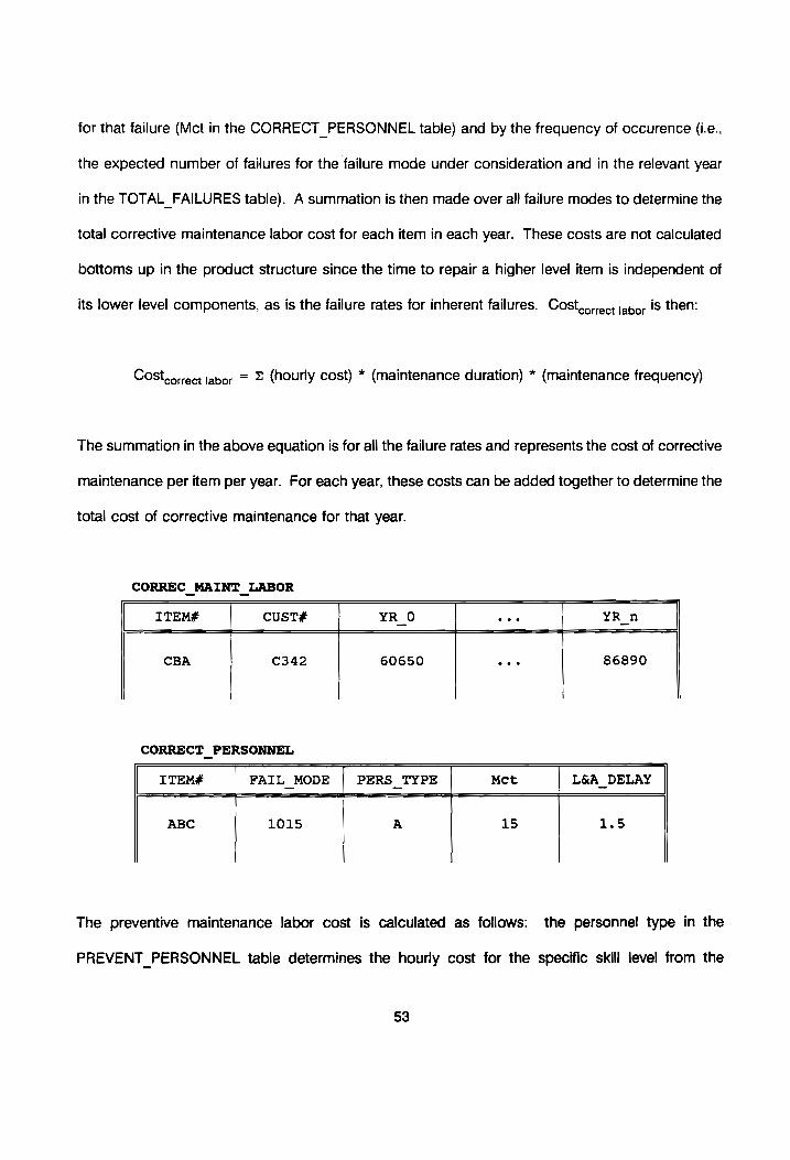
for that failure (Mct in the CORRECT PERSONNEL table) and by the frequency of occurence (i.e.,
the expected number of failures for the failure mode under consideration and in the relevant year
in the TOTAL_FAILURES table). A summation is then made over all failure modes to determine the
total corrective maintenance labor cost for each item in each year. These costs are not calculated
bottoms up in the product structure since the time to repair a higher level item is independent of
its lower level components, as is the failure rates for inherent failures. Cost,, ect jabor is then:
Cost = = (hourly cost) * (maintenance duration) * (maintenance frequency) correct labor
The summation in the above equation is for all the failure rates and represents the cost of corrective
maintenance per item per year. For each year, these costs can be added together to determine the
total cost of corrective maintenance for that year.
CORREC_MAINT LABOR
ITEM# CUST# YR_O .. YR_n
CBA C342 60650 wee 86890
CORRECT_PERSONNEL
ITEM# FAIL MODE | PERS TYPE Mct L&A_DELAY
ABC 1015 A 15 1.5
The preventive maintenance labor cost is calculated as follows: the personnel type in the
PREVENT PERSONNEL table determines the hourly cost for the specific skill level from the
53
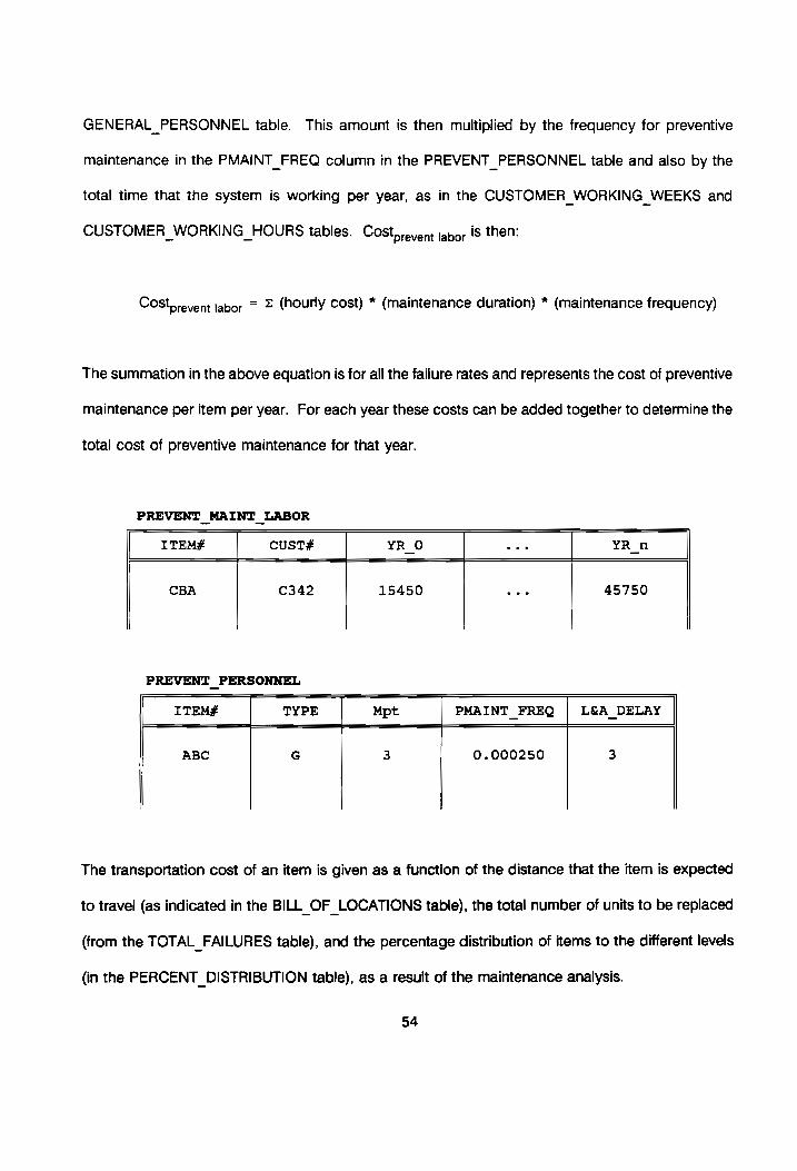
GENERAL PERSONNEL table. This amount is then multiplied by the frequency for preventive
maintenance in the PMAINT_ FREQ column in the PREVENT PERSONNEL table and also by the
total time that the system is working per year, as in the CUSTOMER WORKING WEEKS and
CUSTOMER WORKING HOURS tables. Cost is then: prevent labor
Cost = ~ (hourly cost) * (maintenance duration) * (maintenance frequency) prevent labor
The summation in the above equation is for all the failure rates and represents the cost of preventive
maintenance per item per year. For each year these costs can be added together to determine the
total cost of preventive maintenance for that year.
PREVENT MAINT LABOR
ITEM# cusT# YR_O . YRn
CBA C342 15450 . 45750
PREVENT_PERSONNEL
ITEM# TYPE Mpt PMAINT FREQ | L&A_DELAY
ABC G 3 0.000250 3
The transportation cost of an item is given as a function of the distance that the item is expected
to travel (as indicated in the BILL_OF_LOCATIONS table), the total number of units to be replaced
(from the TOTAL_FAILURES table), and the percentage distribution of items to the different levels
(in the PERCENT_DISTRIBUTION table), as a result of the maintenance analysis.
54
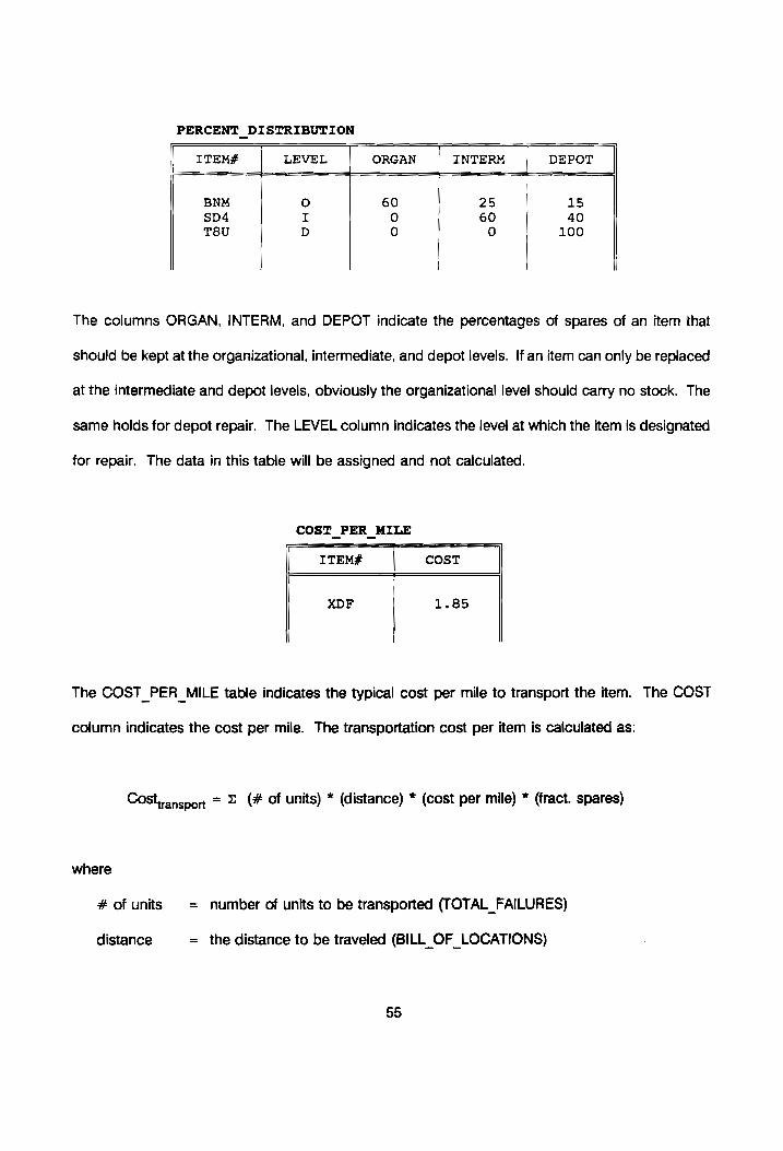
PERCENT DISTRIBUTION
ITEM# LEVEL ORGAN INTERM | DEPOT
|
BNM oO 60 25 15
SD4 I 0 60 40 T8U D 0 0 100
The columns ORGAN, INTERM, and DEPOT indicate the percentages of spares of an item that
should be kept at the organizational, intermediate, and depot levels. if an item can only be replaced
at the intermediate and depot levels, obviously the organizational level should carry no stock. The
same holds for depot repair. The LEVEL column indicates the level at which the item is designated
for repair. The data in this table will be assigned and not calculated.
COST _PER_MILE
Cost
ITEM#
XDF 1.85
The COST _PER_MILE table indicates the typical cost per mile to transport the item. The COST
column indicates the cost per mile. The transportation cost per item is calculated as:
CoStransport = £ (# of units) * (distance) * (cost per mile) * (fract. spares)
where
# of units = number of units to be transported (TOTAL_FAILURES)
distance = the distance to be traveled (BILL_OF_ LOCATIONS)
55

cost of transportation per mile (COST _PER_MILE) cost per mile
fract. spares the fraction of all the units that go to the specific level under consideration
(PERCENT DISTRIBUTION)
The summation in the cost calculation is over all the different levels of repair, with the accompanying
fractions of inventory at each level of repair.
The training cost is given as a total cost per item per year. This value is assigned and maintained
in the TRAINING_COST table. The item number is typically the end item. However, any item that
requires specific training can be specified. A summation gives the total cost of training for each end
item.
TRAINING COST
ITEM# CUST# YR_O eee YR n
CBA C342 75750 eee 185000
The packaging cost is calculated as a function of the number of units that are held in inventory.
The unit packaging cost and the type of packaging required are given in the UNIT_PACKAGE table.
The total package cost per item per year is given in the PACKAGING table.
UNIT_PACKAGE
ITEM#
PACK_TYPE cost
TRG
P34Z
56
64.80

PACKAGING
ITEM#
TRG C342 4536 eee 11458
The shortage cost is not considered since a functional approach is followed. The total cost is
calculated to perform an activity with a certain capacity. The end user, therefore, buys this capacity.
If the system is an item short, the total cost is that of not performing the task with the relevant
Capacity. The number of spare parts to deploy already considers the shortage cost of an item.
The inventory costs are dealt with in the next section.
3.6 INVENTORY ANALYSIS
The primary sources of information in Section 3.6 are: Fogarty and Hoffmann (1983), Naddor (1982),
Reintield (1987), Tersine (1988), and Thomas (1980).
Regarding the management of spare and repair part inventory at the end user, the following are the
four most important parameters and must be determined for each item: 1) Order quantity (Q); 2)
Order interval (T); 3) Reorder point (B); and 4) Safety Stock (S).
The order interval and the reorder point are not always both required. For example, in the fixed
order interval the orders are launched regardless of the size of the current inventory, given that the
need exists. Separate tables exist for these three parameters for each item for the following n years.
In all cases, the column LEVEL indicates the level at which repair takes place. The order quantity
is the number of items that are ordered at the same time and it is maintained in the
57

ORDER_QUANTITY table. The order interval for each item is maintained in the ORDER_INTERVAL
table, and the reorder point in the REORDER _ POINT table.
ORDER_QUANTITY
ITEM# CUST# LEVEL YR_O eee YR
GTX C342 I21 236 173
The order interval is the interval at which orders are placed. It can be presented to the user in
terms of an annual, a monthly, weekly, or daily interval. The original form is in working days but
can be converted into other time periods by the appropriate factors.
ORDER_ INTERVAL
ITEM# CUST#
GTX C342 I21 5.9 eee 4.3
The reorder point is the number of items in inventory that triggers an order for new stock and is
given in units. Whenever the units provide any problem (some material is acquired by length, others
by units, some by volume, etc.), a new field, typically a UNIT OF MEASURE column, can be added
to indicate the unit measure under consideration.
58
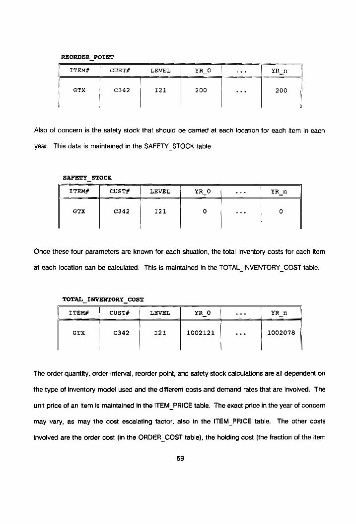
REORDER POINT
ITEM# CUST# LEVEL YR O YR_n
GTX
C342
SAFETY STOCK
I21
200
year. This data is maintained in the SAFETY_STOCK table.
200
Also of concern is the safety stock that should be carried at each location for each item in each
ITEM# CUST# LEVEL YR_n
GTX
C342
I21
Once these four parameters are known for each situation, the total inventory costs for each item
at each location can be calculated. This is maintained in the TOTAL_INVENTORY_COST table.
TOTAL INVENTORY _COST
ITEM# CusST# LEVEL YR_O YR_n
GTX C342 I21 1002121 1002078
The order quantity, order interval, reorder point, and safety stock calculations are all dependent on
the type of inventory model used and the different costs and demand rates that are involved. The
unit price of an item is maintained in the ITEM_PRICE table. The exact price in the year of concern
may vary, as may the cost escalating factor, also in the ITEM_PRICE table. The other costs
involved are the order cost (in the ORDER_COST table), the holding cost (the fraction of the item
59
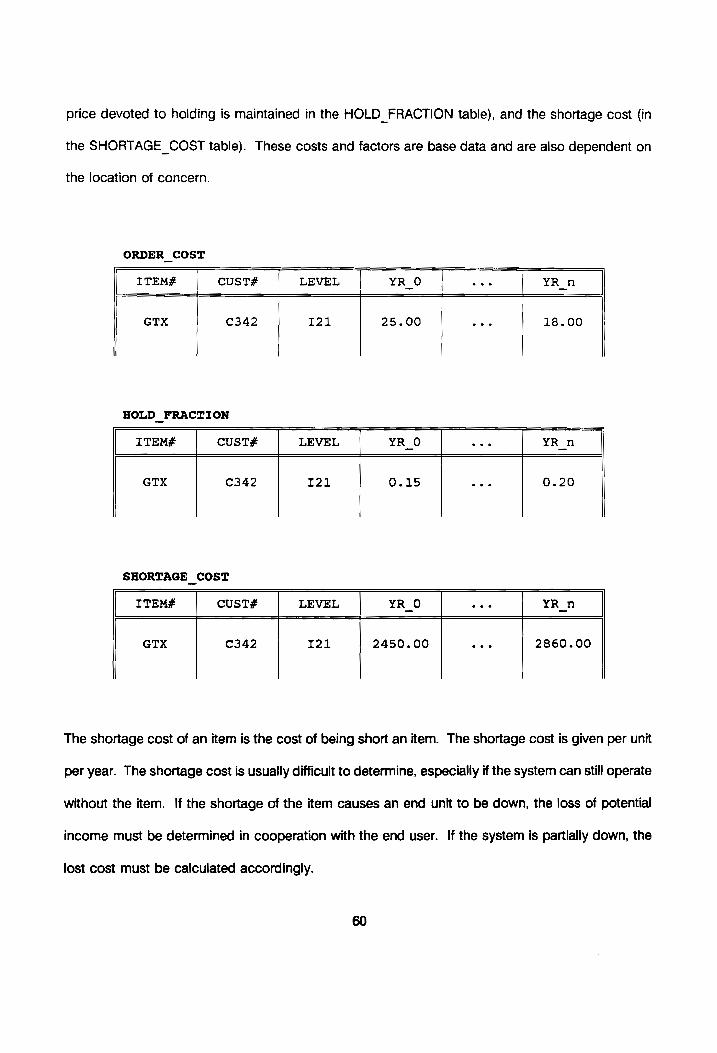
price devoted to holding is maintained in the HOLD FRACTION table), and the shortage cost (in
the SHORTAGE COST table). These costs and factors are base data and are also dependent on
the location of concern.
ORDER _ COST
ITEM#
GTX C342 I21 25.00 18.00
HOLD FRACTION
ITEM# CuST# LEVEL YR_O YRn
GTX C342 I21 0.15 0.20
SHORTAGE COST
ITEM# cUST# LEVEL YR_O YR n
GTX C342 121 2450.00 2860.00
The shortage cost of an item is the cost of being short an item. The shortage cost is given per unit
per year. The shortage cost is usually difficult to determine, especially if the system can still operate
without the item. If the shortage of the item causes an end unit to be down, the loss of potential
income must be determined in cooperation with the end user. If the system is partially down, the
lost cost must be calculated accordingly.

The annual demand rate (R) is a very important parameter in determining inventory levels and costs.
The total number of failures that are expected to occur during each year is the demand rate. These
values are kept in the TOTAL_FAILURES table. The theoretical number of units deployed (in the
UNITS DEPLOYED table) is used since the availability of the system is not known yet. Further,
repair actions are considered to happen instantaneously for the purposes of calculating the demand
rate. The fact that an item can have different reliability characteristics (and, therefore, different
annual demand rates) for different locations, different applications, or different end users can be
overcome by structuring the failure modes intelligently in the FAILURE_MODES table and having
a good configuration management plan.
In order to determine the number of spares that should be carried at each level of repair, the
following procedure is used: From the BILL_OF_ LOCATIONS table and the TOTAL_FAILURES table
all the inherent failures per item that result in replacements are added for all the organizational levels
that belong to each intermediate level. The percentage of the inventory of that item that ts kept at
each level of repair can be obtained from the PERCENT DISTRIBUTION table. The total failures are
then divided accordingly. If the item with a certain failure mode is replaceble at the organizational
level, then the number of spares to be deployed at each organizational site will be divided in the
same proportion to the number of failures at each location. The PERCENT_DISTRIBUTION table
determines the percentage of the total number of spares (as a result of the demand at each
deployment location) that will be carried at the different levels of repair. The costs involved (order,
shortage and holding costs) are initially weighted in the same fashion to establish the global
requirements. After the number of spares at each location is calculated, the exact costs will be
calculated accordingly. If the difference in cost is significant, the system must be modelled again
with the actual costs (explained in chapter 4).
61

The inventory model used for each item is depicted in the INV_ITEM MODEL table. An exhaustive
list of models used is given in the INV MODEL LIST table. The TYPE column in the
INV_ITEM_MODEL table refers to the TYPE column in the INV MODEL LIST table. Again, the
LEVEL column in the INV_ITEM_MODEL table refers to the specific level or channel of maintenance.
INV_ITEM_ MODEL
ITEM# LEVEL TYPE
GTX 121 Cc
INV_MODEL LIST
TYPE DESCRIPTION
A ECONOMIC ORDER QUANTITY : NO STOCKOUTS B ECONOMIC ORDER QUANTITY : STOCKOUTS ALLOWED Cc ECONOMIC MANUFACTURING QUANTITY D ECONOMIC ORDER INTERVAL E LOT-FOR-LOT F PERIODIC ORDER QUANTITY G PART-PERIOD ALGORITHM H PROB.: VARIABLE DEMAND & CONSTANT LT (K KNOWN) I PROB.: VARIABLE LT & CONSTANT DEMAND (K KNOWN) J PROB.: VARIABLE DEMAND & VARIABLE LT (K KNOWN) K PROB.: STOCKOUT COSTS UNKNOWN
The Economic Manufacturing Quantity (EMQ) is used as an example of how the inventory is
analyzed. The EMQ is only of concern if the end user produces some of the items himself. The
order quantity, order interval, reorder point, and total annual cost (TC) are calculated for the EMQ
model as follows:
62

Qa" =| i H(p - r)
2C p
T= [{—}{i—-}}" HR p-r
RL
B= [—] N
RC HQ" (p - r) TC = RP +— + ——__
Q 2p
N is typically 250 active workdays per year. However, the user needsto be prompted how many
days per year he works. This number must be consistent with the total number of hours that he
works per year, which is given in the CUSTOMER_WORKING HOURS and
CUSTOMER_WORKING_WEEKS tables. The lead time L is in calander days. The production rate
is p, and r is the demand rate. The demand rate R is a function of the reliability of the item and is
the amount in the TOTAL_FAILURES table. The production rate is given by the user in the
EMQ_ PRODUCTION table. Although the end user can manufacture an item at various locations at
the same time, only the total production quantity is considered. Both p and r have the dimensions
units-per-day. PROD_RATE and PROD_COST represent the production rate and the unit production
cost, both in working days.
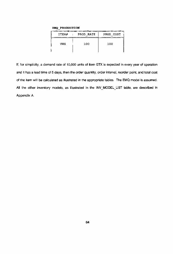
EMQ PRODUCTION
ITEM# ' PROD RATE PROD COST
VWX 100 100
lf, for simplicity, a demand rate of 10,000 units of item GTX is expected in every year of operation
and it has a lead time of 5 days, then the order quantity, order interval, reorder point, and total cost
of the item will be calculated as illustrated in the appropriate tables. The EMQ model is assumed.
All the other inventory models, as illustrated in the INV_MODEL LIST table, are described in
Appendix A.
4.0 A HEURISTIC PROCEDURE FOR SYSTEM DESIGN
A heuristic procedure is proposed to approach the optimum solution to system and logistic design.
This heuristic procedure utilizes a process of enumeration and is used in conjunction with the
database management system developed in Chapter 3. This heuristic procedure does not
guarantee optimality. However, a solution close to the “optimum” solution will be reached. After
reaching this solution, the user can change the value of any parameter listed in Paragraph 2.10 and
the resultant effect on the entire system will be made visible.
Relationships are defined between the user requirements, the reliability and maintainability of the
system, the number of units deployed, the inventory level, and other logistic requirements of the
system. The heuristic procedure is used to interactively manipulate these parameters to obtain a
good solution to the problem. Technical performance and cost measures are used as criteria. The
output of the heuristic procedure is a specification of:
1. The number of end items to deploy at each location.
2. The inventory level for each item at each location.
3. The reorder point for each item in inventory at each location.
4. The throwaway age for each item of each configuration of prime equipment and inventory.
(Items are considered from end items to the lowest level replaceable items.)
5. The identification of all test and support equipment, facilities, personnel, documentation,
training, and packaging requirements for each design configuration for each facility at each
level of repair.

The heuristic procedure will also determine, under each set of conditions, which items will contribute
most to the effectiveness of the system (see Paragraph 4.3) if additional units of those items are
added to the inventory. The major assumptions of this heuristic procedure are as follows:
1. All corrective maintenance actions involve the replacement of items. Each repairable item
that has been removed due to a failure can be repaired (or replaced) at whatever level of
concern. Items that are replaced at one level and the faulty repairable item is sent to
another level for repair, will have at least two failures modes. The first failure mode,
typically starting with the digit 8, requires the initial replacement of the item. The second
failure mode, typically on a lower level itern than the original iter, will be associated with
the relevant level of repair in the REPAIR_LEVEL table.
2. Whenever the inventory level of an item drops to zero and demand still exists, spare parts
are ordered immediately. This means that the longest time period that the system can be
down due to shortages is equal to the lead time of the item that caused the delay.
3. Time between visits to a repair facility is uniformly distributed.
4. The only difference between the achieved availability and the operational availability is the
time that the system is down due to a shortage of spare parts.
5. The total failure rate per year depends on (among other things) the number of units
deployed and the time the equipment is operational. The number of units deployed
depends on the operational availability of the end item (because of the maintenance
requirements of the system). The operational availability again depends on the failure rate
66

of the system. A loop has now been defined. The assumption made is that the operational
availability of the system, as calculated in each iteration, will be used to determine the total
failure rate of the system in each subsequent iteration. This is a realistic assumption since
the effect of each iteration on the system is very small. When a final solution has been
reached, a few more iterations can be run on the same configuration to stabilize the results.
4.1 TOTAL NUMBER OF FAILURES PER YEAR
For time-independent failures and for time-dependent failures, the total number of failures per year
for each failure mode (FM) for the j” item (@em) is given in [4.1] and [4.2] respectively:
(# units deployed); * A, * %.rx4/nr * (hours worked per year) [4.1] 2M j
®.eM = ®t (# units deployed); * A, * hours worked per year] [4.2]
The (# units deployed); is the number of units of item j that are deployed. This is calculated from
the number of items utilized per end item deployed (in the UNITS_DEPLOYED table), multiplied by
the quantity used per end item (in the PRODUCT_STRUCTURE table), multiplied by the fraction of
the time the unit is utilized (in the MISSION_FRACTION table). ;.-44/p, is the failure rate per hour
for the particular failure mode for the j"" item. The values of ®;.Fy are all the failures that demand
replacements and are maintained in the TOTAL_FAILURES table. The total failure rate per item per
year, ©, is the summation of all the different failure modes for each item. This is calculated in [4.3]:
(FM) max &= = ®.eu [4.3]
67

The preventive maintenance frequency per hour for the Kk” item (fpt, jn) is maintained in the
PMAINT FREQ column of the PREVENT PERSONNEL table. The total number of preventive
maintenance actions per item per year (fpt,) is calculated from [4.4]:
fpt, = (# units deployed), * A, * fpt,,, * (hours worked per year) [4.4]
The “hours worked per year’ in both preventive and corrective cases are the total number of hours
that the end user would like the equipment to work. These are constant values and are maintainded
in the CUSTOMER_WORKING_HOURS and CUSTOMER_WORKING_WEEKS tables, both as a
function of time. The values of 7 and fpt, are initially calculated for a system with just enough units
deployed (fractions allowed) to fulfill the user requirements for each year, given that the operational
availability of the system is 1.0. This number of units is the theoretical number of units deployed
in the UNITS _DEPLOYED table. Although not stated specifically, the values of ®; and fpt, are all
calculated per location as a result of the user requirements in the DETAIL_REQUIREMENTS table.
In order to fulfill the user requirements, sufficient capacity must be made available at each location
to meet the demand. This can be calculated from [4.5]:
Capacity Available = (# end-items deployed) * A, * (Unit capacity) [4.5]
The unit capacity values are maintained in the ITEM_CAPACITY table. Unit capacity is an inherent
characteristic of an item and is not a function of the number of units deployed. For the rest of this
chapter, all calculations are done on a “per year" basis. The unit capacity in (4.5] is the unit
capacity per year, and the available capacity is also per year (in response to capacity required per
year).
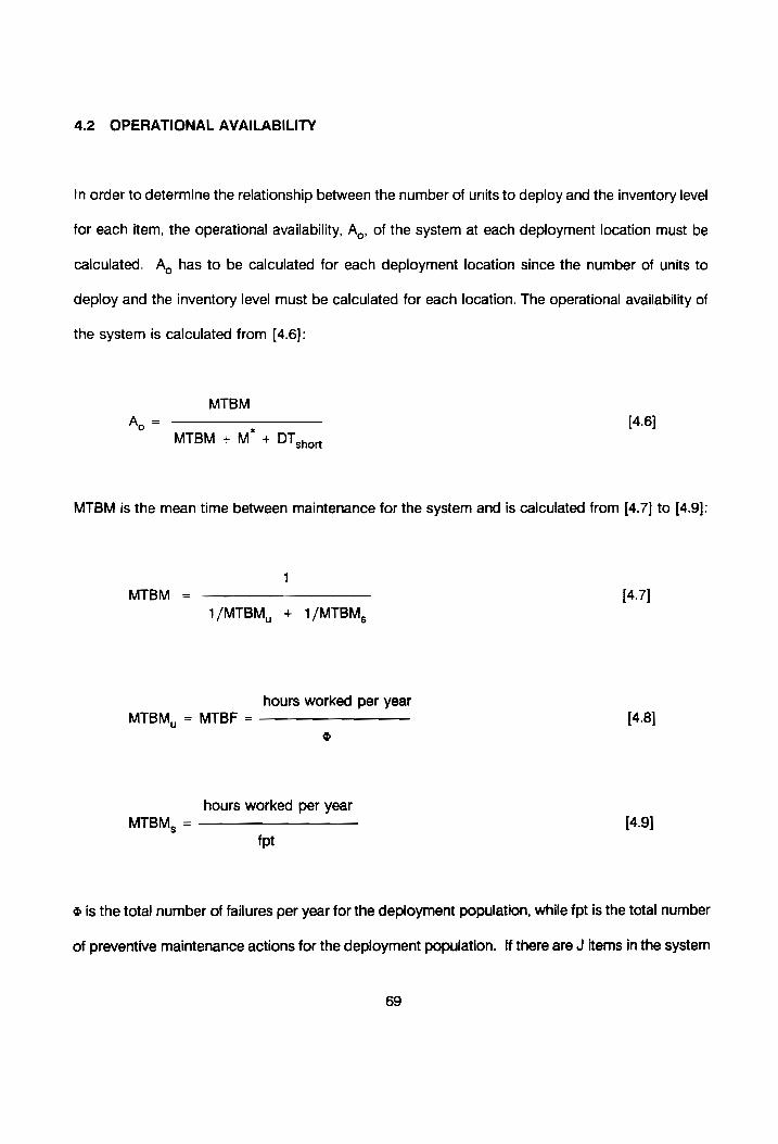
4.2, OPERATIONAL AVAILABILITY
In order to determine the relationship between the number of units to deploy and the inventory level
for each item, the operational availability, A,, of the system at each deployment location must be
calculated. A, has to be calculated for each deployment location since the number of units to
deploy and the inventory level must be calculated for each location. The operational availability of
the system is calculated from [4.6]:
MTBM A, = - [4.6]
MTBM + M* + DT spon
MTBM is the mean time between maintenance for the system and is calculated from [4.7] to [4.9]:
1 MTBM = [4.7]
1/MTBM, + 1/MTBM,
hours worked per year MTBF = [4.8]
®
MTBM, it
hours worked per year
i MTBM, [4.9] fpt
@ is the total number of failures per year for the deployment population, while fpt is the total number
of preventive maintenance actions for the deployment population. If there are J items in the system
69
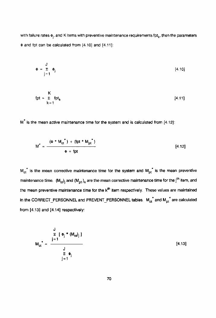
with failure rates ©, and K items with preventive maintenance requirements fpt,, then the parameters )
® and fpt can be calculated from [4.10] and [4.11]:
J @= 2 & [4.10]
K fpt= = fpt, 14.11]
M° is the mean active maintenance time for the system and is calculated from [4.12]:
— (* My) + (fpt * Moe) M” = ; [4.12]
© + fpt
Ma is the mean corrective maintenance time for the system and Mo, is the mean preventive
maintenance time. (Mex); and (Mo ), are the mean corrective maintenance time for the j* item, and
the mean preventive maintenance time for the Kk" item respectively. These values are maintained
in the CORRECT_PERSONNEL and PREVENT_PERSONNEL tables. M,, and M,,. are calculated
from [4.13] and [4.14] respectively:
My = ——————— [4.13]
70

[ ft, * (Moy )k J k=1
M.,. = ————————_—— [4.14] K = fpt, k=1
DT snort is the downtime in the system as a result of the unavailability in spare parts. DT,.,,, is the sho
summation of all the downtimes as a result of shortages of all the items in the system. The
parameter downtime, will denote the downtime of the system due to a shortage of the j* item. The
end item comprises J different replaceable items. DT,.,,, is then calculated from [4.15]: sho
qc
DT snort = 2 downtime; [4.15] J=
where downtime, is the product of 1) the probability of having demand in excess of the number of
items (N) carried in stock for item j over the period MTBM, and 2) the lead time of the j* item, LT;.
The Poisson distribution can be used to determine the probability of demand for item j over the
period MTBM. The amount by which the demand exceeds the available inventory (Ni) for item j
during the period MTBM, is denoted by n,. downtime, is calculated from [4.16]:
@o
downtime; = = Prob (demand tam) = Nj + n) * LT,
nj=1
N. j
= LT, * {1- = Prob (demandiiytay) = 7)} nj=0
71

N, (®, * MTBM)”! . =LT*{1- 5 ———— * @ i" MTBM)) [4.16]
The operational availability A, can now be calculated by substituting equations [4.7] to [4.16] into
[4.6]. The relationship between the number of units deployed and the inventory level is now
defined.
4.3. THE HEURISTIC PROCEDURE
There are two approaches in using the heuristic procedure. Both approaches utilize a process of
enumeration. The difference between the two is in the starting point. The first approach first
determines the minimum number of units to deploy that will fulfill the need, assuming a virtually
unlimited supply of inventory as a starting point. The deployment population is then progressively
increased, and the inventory is each time “loaded" from a zero level to determine the most effective
level of inventory that needs to accompany a deployed population to fulfill the requirements at the
lowest equivalent cost.
The second heuristic first determines a reasonable solution (not necessarily a feasible solution) of
the deployed population and the inventory. It then determines which items can be added to the
inventory and which ones can be subtracted to increase the cost effectiveness of the system, while
still fulfilling the requirements. Different deployment configurations around the initially suggested
configuration are also considered. Each deployment configuration of end-items and inventory is
evaluated as in the first heuristic. The second approach, although not as accurate as the first, will
demand much less computing time.
72

4.3.1 The First Heuristic Procedure
The minimum possible number of units to deploy (which will fulfill the requirements) is first
determined. Steps 1 through 10 determine the minimum number of units to deploy. The numbers
in parenthesis refer to the specific equations. The first heuristic procedure is as follows:
1. Let A, = 1.0.
2. Set the capacity available in [4.5] equal to the required capacity. Calculate the number of
units to deploy, using [4.5].
3. Determine the failure rate of each item [4.3], using [4.1] and [4.2], and the failure rate of
the system, [4.10].
4. Determine the number of preventive maintenance actions per year for each item [4.4], and
for the system, [4.11].
5. Determine the MTBM [4.7], using [4.8] and [4.9].
6. Determine M" [4.12], using [4.13] and [4.14].
7. Assume DT.454 = 0.0 [4.15].
8. Calculate A, [4.6].
73

10.
Recalculate the number of units deployed with new A,, again using [4.5].
Repeat steps 3 to 9, using A, as calculated in step 9. Add one unit to the suggested
population to be deployed.
Up to this point, a virtually infinite inventory level was assumed (DT,,,, = 0). The inventory is now
depleted (in the model) and will now be "loaded" from a zero level. This loading process is
described in the following steps:
11. For each component j of the end item, calculate the Gain Ratio as the ratio between the
gain in operational availability of the system if an additional unit of item j is added to
inventory, and the unit acquisition cost of item j. The true gain ratio would involve the total
life-cycle cost. This cost is, for the purposes of determining the most likely items to be
added to inventory, approximated by the acquisition cost. The item with the biggest Gain
Ratio is the candidate that will have the biggest increase in the cost effectiveness of the
system if one unit of that item is added to inventory.
Gain in A, Gain Ratio; = [4.17]
Unit acquisition cost;
First, DT,5, is calculated for each item [4.16] and the system [4.15] with zero inventory
(N; = 0). A, is calculated, using DT... and the results from step 10. This A, serves as
a baseline. DT.,, is now calculated for each item in the product configuration under
consideration if one unit of that item is added to the inventory. For each item added to
inventory, the new A, is calculated. The difference in this newly calculated A, and the
74
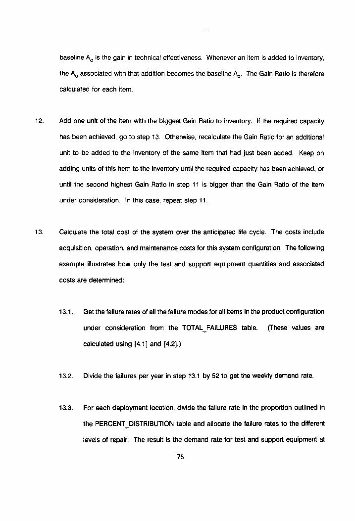
12.
13.
baseline A, is the gain in technical effectiveness. Whenever an item is added to inventory,
the A, associated with that addition becomes the baseline A,. The Gain Ratio is therefore
calculated for each item.
Add one unit of the item with the biggest Gain Ratio to inventory. If the required capacity
has been achieved, go to step 13. Otherwise, recalculate the Gain Ratio for an additional
unit to be added to the inventory of the same item that had just been added. Keep on
adding units of this item to the inventory until the required capacity has been achieved, or
until the second highest Gain Ratio in step 11 is bigger than the Gain Ratio of the item
under consideration. In this case, repeat step 11.
Calculate the total cost of the system over the anticipated life cycle. The costs include
acquisition, operation, and maintenance costs for this system configuration. The following
example illustrates how only the test and support equipment quantities and associated
costs are determined:
13.1. Get the failure rates of all the failure modes for all items in the product configuration
under consideration from the TOTAL_FAILURES table. (These values are
calculated using [4.1] and [4.2].)
13.2. Divide the failures per year in step 13.1 by 52 to get the weekly demand rate.
13.3. For each deployment location, divide the failure rate in the proportion outlined in
the PERCENT DISTRIBUTION table and allocate the failure rates to the different
levels of repair. The result is the demand rate for test and support equipment at
75

each level of repair.
13.4. For each failure mode and item, at each repair facility, determine the type and
quantity of test and support equipment required as a function of the demand rate,
as calculated in step 13.3.
13.5. The requirements for test and support equipment are summarized and rounded up
for all the test and support equipment that are commonly used at a repair facility.
13.6. The quantity and type of test and support equipment have now been defined. The
quantity of each type of test and support equipment is multiplied by the the unit
price of the equipment in the ITEM PRICE table. The requirements and cost for
test and support equipment at each repair facility are now defined. This process
is repeated for the other elements of logistics.
14. Add one end item to the system and deplete the inventory. Repeat steps 3 to 6 and 11 to
13. Repeat these steps until the lowest present equivalent life-cycle cost has been
obtained. The deployment configuration associated with this cost is the preferred
alternative.
The item that will have the biggest positive influence on the cost effectiveness of the system if
additional stock of that item is carried, is the item with the biggest Gain Ratio. The optimum
throwaway age will be when the ratio of the increase in operational availability to the present
equivalent life-cycle cost of the new item exceeds that of the old item. Once the overall system level
requirements are established for inventory, local lot sizing technics can be used to determine the
76

exact order quantities and reorder points.
4.3.2 The Second Heuristic Model
The same enumeration process is followed as in the previous heuristic approach, except that a
better starting point is defined. This is done by initially assuming that 1) no more capacity will be
utilized than required by the end user; and 2) enough capacity will be made available to fulfill the
need. This means that the total number of failures in the system remains constant, regardless of
the number of units deployed. The maintenance requirements also remain constant. The local
optimum probability of stockout (as defined by Johnson and Montgomery, 1974) is determined for
each item:
. Ha P, =—
KR
where
H = holding cost
Q = economic order quantity
K = stockout cost
R = demand rate
The downtime of each item, and the system, are calculated directly from these probabilities, using
[4.16] and [4.15]. The deployment population can now be estimated (because of the initial
assumptions). The Gain Ratio of each item is determined. Inventory is now reduced for the items
with the least Gain Ratios, and inventory is added for those with the biggest Gain Ratios until the
process stabilizes. If the required capacity had not been achieved when the process had stabilized,
77

more inventory must be added. Different simulations are also run with different numbers of end
items deployed.
4.4 AN EXAMPLE
The following simple example illustrates some of the capabilities of the proposed model. A system,
consisting of only two replaceable items, is considered. The primary objective is to determine the
number of end-items to deploy, as well as the number of spare parts for each of the two items of
the system. One of the items, item A, is then improved by redesign. The resultant impact on the
system is subsequently analyzed. Although the procedure illustrated in this example is only one of
many different ways of manipulating data within the framework of the proposed model, it shows
what will typically be done in analyzing new data. System XYZ is illustrated in Figure 5 and is
defined accordingly in the PRODUCT STRUCTURE table.
XYZ
A B
Figure 5 Product structure of system XYZ
PRODUCT STRUCTURE
PARENT CHILD QTY PER
XYZ A 1 XYZ B 1
78
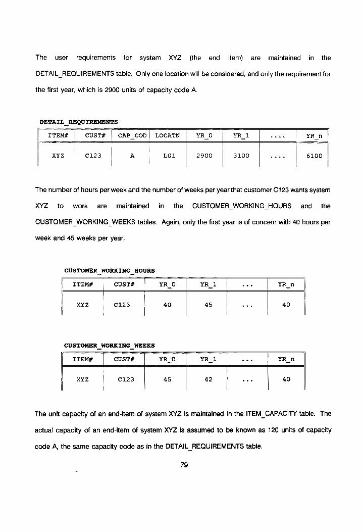
The user requirements for system XYZ (the end item) are maintained in the
DETAIL REQUIREMENTS table. Only one location will be considered, and only the requirement for
the first year, which is 2900 units of capacity code A.
DETAIL REQUIREMENTS
| ITEM# CUST# CAP_COD| LOCATN YR_O YR 1 wees YR_n
XYZ C123 A LO1 2900 3100 see. 6100
The number of hours per week and the number of weeks per year that customer C123 wants system
XYZ to work are maintained in the CUSTOMER_WORKING HOURS and _ the
CUSTOMER_WORKING_WEEKS tables. Again, only the first year is of concern with 40 hours per
week and 45 weeks per year.
CUSTOMER_WORKING HOURS
ITEM# cust# YR_O
XYZ C123 40 4s ees 40
CUSTOMER_WORKING_WEEKS
ITEM# CUST# YR_O YR_1 eee YR n
XYZ C123 45 42 eee 40
The unit capacity of an end-item of system XYZ is maintained in the ITEM_CAPACITY table. The
actual capacity of an end-item of system XYZ is assumed to be known as 120 units of capacity
code A, the same capacity code as in the DETAIL_REQUIREMENTS table.
79
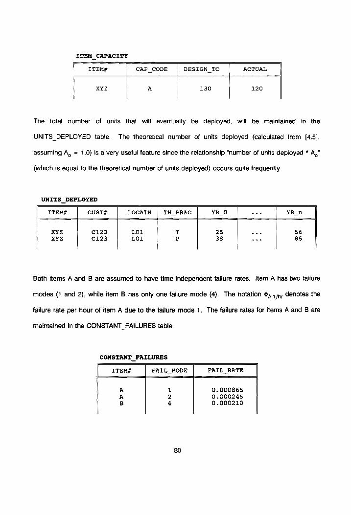
The total number of units that will eventually be deployed, will be maintained in the
UNITS DEPLOYED table.
assuming A, = 1.0) is a very useful feature since the relationship "number of units deployed * A,"
(which is equal to the theoretical number of units deployed) occurs quite frequently.
ITEM CAPACITY
ITEM# CAP_CODE DESIGN_TO ACTUAL
XYZ
UNITS DEPLOYED
A
The theoretical number of units deployed (calculated from [4.5],
130 120
ITEM# custT# LOCATN | TH_PRAC YR_O wee YR n
XYZ C123 LO1 T 25 eee 56 XYZ C123 LO1 P 38 wee 85
Both items A and B are assumed to have time independent failure rates. Item A has two failure
modes (1 and 2), while item B has only one failure mode (4). The notation ©,.,/,, denotes the
failure rate per hour of item A due to the failure mode 1.
maintained in the CONSTANT FAILURES table.
CONSTANT FAILURES
ITEM# FAIL MODE FAIL_RATE
A 1 0.000865 A 2 0.000245 B 4 0.000210
The failure rates for items A and B are
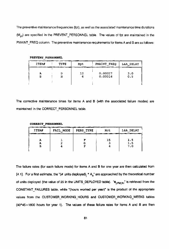
The preventive maintenance frequencies (fpt), as well as the associated maintenance time durations
(M,,) are specified in the PREVENT PERSONNEL table. The values of fpt are maintained in the
PMAINT FREQ column. The preventive maintenance requirements for items A and B are as follows:
PREVENT _ PERSONNEL
ITEM# TYPE Mpt PMAINT FREQ L&A_ DELAY
A D 12 0.00027 3.0
B H 6 0.00014 0.5
The corrective maintenance times for items A and B (with the associated failure modes) are
maintained in the CORRECT PERSONNEL table.
CORRECT PERSONNEL
ITEM# FAIL MODE PERS TYPE Mct L&A_DELAY |
A 1 F 15 1.5 A 2 G 3 1.5
4 F 4 7.0
The failure rates (for each failure mode) for items A and B for one year are then calculated from
[4.1]. Fora first estimate, the "(# units deployed), * A," are approached by the theoretical number
of units deployed (the value of 25 in the UNITS_DEPLOYED table). "&;.r14/,," is retrieved from the
CONSTANT_FAILURES table, while “(hours worked per year)" is the product of the appropriate
values from the CUSTOMER_WORKING_HOURS and CUSTOMER_WORKING_WEEKS tables
(40*45=1800 hours for year 1). The values of these failure rates for items A and B are then
81

determined to be:
The TOTAL_FAILURES table is then updated with these values. This table then looks as follows:
= 38.3
= 10.8
= 9.3
TOTAL FAILURES
The total failure rate per item per year, as well as the total failure rate per year of the end item XYZ,
are then calculated from [4.3] and [4.10]. Tables do not exist for these failure rates; it is calculated
as needed. These failure rates are then calculated to be:
$n = 9.3
® = 58.4
The same principles are followed in calculating the preventive maintenance frequencies. The only
real difference is that each item has only one “failure mode" for preventive maintenance. The
preventive maintenance frequencies are calculated from [4.4] and [4.11] to be:
82
ITEM# FAIL MODE LOCATN YR_O YR_1 oe YR_n
A 1 LO1 38.3 45.9 ose 54.8 A 2 LO1 10.8 15.0 eee 19.7 B 4 LO1 9.3 12.6 eee 14.4

fpt, = 12.0
fpt = 18.2
In order to calculate the operational availability of the system from [4.6], the MTBM is first calculated
from [4.8] and [4.9]. The required parameters are all known at this point. The results are:
MTBM,, = 1800/58.4 = 30.8
MTBM, = 1800/18.2 = 98.9
MTBM = 23.5
The maintenance times are calculated from [4.12], [4.13], and [4.14]. Again, all the required
variables are known. The maintenance times are then calculated to be:
My = 11.0
Mot = 10.0
M = 10.8
The achieved availability can now be calculated from [4.6] (where the downtime is initially assumed
zero):
A, = 0.685
The operational availability will be less than the achieved availability since the latter assumes an
infinite supply of inventory. For simplicity, it is assumed that all spare parts will have inventory levels
83

such that the probability of having a spare part available upon request is at least 0.90. To have
more manageable quantities, the annual failure rates will be converted to monthly failure rates. The
operational availability calculation will therefore also be transformed to accommodate an MTBM of
160 hours. The demand for spare parts and the associated probability of occurrence can now be
determined from the Poisson distribution in [4.16]. The only unknown in [4.16] is the lead time.
If an item is defined to the system, the lead time is a required data field in the ITEM PRICE table.
The lead time is therefore retrieved from the ITEM_PRICE table. The cumulative demand distribution
for items A and B are then calculated as follows:
Dy Prob, fe Probe
0 0.0167 0 0.4584
1 0.0852 1 0.8160
2 0.2252 2 0.9554
3 0.4161
4 0.6113
5 0.7709
6 0.8797
7 0.9433
Assume item A has a lead time of 4 weeks (160 hours) and item B has a lead time of 2 weeks (80
hours). DT.,., and the operational availability A, can now be calculated from [4.16] and [4.6]
respectively, assuming for simplicity a requirement of 0.90 of having a spare part available upon
request. These values are then calculated to be:

DT snot = {(1 - 0.9433) * 160} + {(1 - 0.9554) * 80}
12.64 > i 160 / (160 + 73.5 + 12.64)
0.65
Since A, is now known, the actual number of end items to deploy can now be calculated from [4.5]
to be:
2900 = Nyyz * 0.65 * 120
38 units to deploy of system XYZ Nxyz
N, = 7 spares for item A
Ng = 2 spares for item B
From [4.5], the total available capacity is 2964. The UNITS_DEPLOYED table is now updated with
the "practical" number of units deployed. Tables for spare parts do not exist; the spare parts are
calculated as needed.
item A is now redesigned and test data reveal the following hourly failure rates, together with the
new preventive maintenance requirements:
©p.o/n. = 0.00015
fpt, = 0.00018
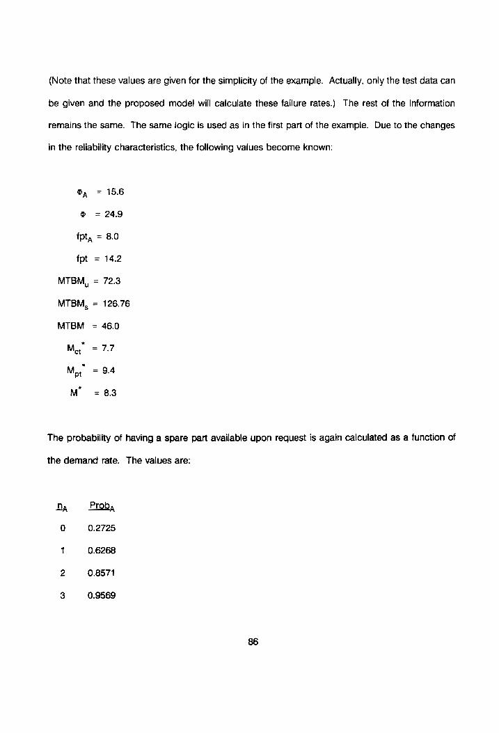
(Note that these values are given for the simplicity of the example. Actually, only the test data can
be given and the proposed model will calculate these failure rates.) The rest of the information
remains the same. The same logic is used as in the first part of the example. Due to the changes
in the reliability characteristics, the following values become known:
@, = 15.6
@ = 249
fpt, = 8.0
fpt = 14.2
MTBM,, = 72.3
MTBM, = 126.76
MTBM = 46.0
Ma = 7-7
Mo = 9.4
M =83
The probability of having a spare part available upon request is again calculated as a function of
the demand rate. The values are:
Da Prob,
0 0.2725
1 0.6268
2 0.8571
3 0.9569

if the same restriction holds that all items must have a probability of meeting demand of at least
0.90, then A, increases to 0.803 and the available capacity increases to 3660 while only 3 spares
of item A is carried (compared to 7 previously). If the restriction of a 0.90 probability of meeting
demand does not hold, the most economical system must be designed. Several different
combinations of spare parts will be evaluated. For the deploymed population of 38 end items, the
following combinations of spare parts will result in the operational availabilities and available
Capacities exhibited:
Alternative A B Ao Capacity Acceptable
1 1 0 0.55 2508 N
2 1 1 0.61 2782 N
3 1 2 0.63 2894 N
4 1 3 0.64 2927 Y
5 2 0 0.63 2872 N
6 2 1 0.71 3221 Y
7 3 0 0.67 3048 Y
For simplicity, the total annual equivalent life-cycle cost of each item is approximated by its unit
cost. The following selection criteria hold for the above case: If the unit cost of item A is more than
that of item B, choose alternative 4. If B is more expensive than A, choose alternative 7. However,
a cost analysis can be done to evaluate the increase in available capacity if alternative 6 is
considered.
The number of end items to deploy can now be altered and the inventory can be determined for
each deployment configuration. The system that has the lowest annual equivalent life-cycle cost
87

is the preferred approach. Once the overall inventory requirements are established, the inventory
models are used to determine the exact quantities and frequency of procurement.
The user can change any parameter value by entering the new value in the appropriate field and
the proposed model will automatically recalculate the desired output. The values that can be
changed relevant only to this example include:
1. Product structure (replace item A with another item, or series of items).
2. The number of units that are used in each level of the product structure.
3. Customer requirements (capacity and work time).
4. ltem unit capacity.
5. Item failure rate.
6. Maintainability characteristics.
7. Number of units deployed.
8. Number of spare parts deployed.
This is a very simple example that covers only a portion of the capabilities of the proposed relational
database management system. When systems become large (consisting of thousands of items) and
each item has several parameters that could potentially influence the sytem, the proposed model
will still keep track of all changes, as well as the effect of each change on the system.
5.0 SUMMARY, CONCLUSIONS, AND EXTENSIONS
The procedure developed in this research is summarized in this chapter. Also, some conclusions
are made as to the strengths of the proposed model and further research opportunities are
identified.
5.1 SUMMARY
The objective of this research was to define a relational database management system that will
enable the user of it to evaluate different possible design configurations of complex systems in such
a way that the required system effectiveness will be achieved at a close-to-minimum life-cycle cost.
Also, the logistic requirements are defined for each design configuration. The relational database
management system will also provide the user with the capability to test the sensitivity of the system
due to changes in input variables. The decision variables are mainly the number of end items to
deploy, the inventory level of spare and repair parts, the reorder points and order quantities of
inventory, the throwaway age of items, and other logistic requirements for the system.
The methodology utilized is noted in the following steps: Customer requirements are analyzed in
functional terms. Feasible design alternatives are considered and defined as product configurations.
The reliability characteristics of each product configuration are determined. Initially, these reliability
values are allocated from a system-level down to lower level components, and later determined from
test and evaluation data. A maintenance analysis is conducted to determine the inventory
requirements (using reliability data) and the other logistic requirements for each design
configuration.

A vector of effectiveness measures can then be developed for each customer, depending on
objectives, constraints, and risks. These effectiveness measures, consisting of a combination of
performance and cost measures, are used to aid objectively in deciding which alternative is
preferred.
5.2 CONCLUSIONS
The contribution of this research can be summarized as follows: The objective of defining a
relational database management system is met. The database management system was not coded
(it was not part of the objective). It is therefore not possible to state with certainty that such a
database system will definitely fulfill all the requirements stated. However, the flow of logic was
tested several times. One such an example was illustrated in Paragraph 4.4. The proposed model
attempts to establish the design so that the required effectiveness will be achieved at a minimum
life-cycle cost.
The proposed model does not guarantee optimality. However, the heuristic procedure utilized in
Chapter 4 gives a practical solution close to the optimum. After reaching this point, the user of the
proposed model will be able to change any input parameter listed in Paragraph 2.10, and the effect
on the whole system will be made visible. Furthermore, for each design configuration the spare and
repair parts are determined that, when added to inventory, will increase the availability of the system
most effectively. This is a dynamic process in that the items that will increase the availability of the
system most effectively are not only a function of the product configuration, but also of the inventory
status. The ability is created to keep track of this dynamic process.
The total life cycle of a system is covered. The proposed model will therefore serve as a central
90
source of information not only over the life cycle of each specific system, but as a common source
of information. Baseline comparisons with other projects are therefore possible. Because a
relational database approached is used, any additional information required (which is not covered
in this research), can be added onto the proposed model. The modelling capability is therefore very
adaptable to changing requirements.
The proposed model will serve as a good management tool since the user will have visibility of the
impact on the system over the life cycle if changes are proposed to the system. Any query can be
constructed that involves any of the parameters in any logical combination modelled. The user will
be able to respond quickly and effectively to customer demands. Another benefit of the proposed
model is that changes can be made to any data, and all other data linked to the original data item
will be updated accordingly.
5.3 FURTHER RESEARCH
Several future research opportunities exist. These are:
1. A more efficient heuristic procedure should be developed to approach the optimum
solution. Although the heuristic procedure proposed herein is effective, it is inefficient since
the boundary lines within which it moves in its search for better solutions are very wide.
The result is a requirement for high computation capability.
2. A uniform distribution is assumed for the time between visits to repair facilities. Queuing
theory should be applied to more effectively determine the actual facility resource
requirements. Simulation software, like SLAM and SIMAN, could be used to model
91
resource requirements.
A weakness of this research is that the relationship between the proposed model and
Computer-Aided Acquisition and Logistic Support (CALS) is not defined. This interface
should be defined in order to accommodate the entire relevant industry in the evaluation
of alternatives.
Although Appendix B touches on the relationship between the proposed model and
Manufacturing Planning and Control, this interface can be refined further. This interface is
important since this research covers the entire lite cycle of a system and that includes
manufacturing.
92

10.
11.
12.
13.
14.
15.
16.
17.
18.
19.
BIBLIOGRAPHY
Ascher, H. and Feingold, H., Repairable systems reliability, Marcell Dekker, 1984.
Aven, T., Reliability achievement: the commercial incentive, Elsevier Science Publishers, 1989.
Bain, L.J., Statistical analysis of reliability and life cycle models, Marcel Dekker, 1978.
Bazovsky, |., Reliability theory and practice, Prentice Hail, 1961.
Bedworth, D.D. and Bailey, J.E., Integrated production control systems, John Wiley & Sons, 1987.
Blanchard, B.S., Logistics engineering and management, Prentice Hall, 1992.
Blanchard, B.S., Systems engineering management, John Wiley & Sons, 1991.
Blanchard, B.S. and Fabrycky, W.J., Systems engineering and analysis, Prentice Hall, 1990.
Carter, A.D.S., Mechanical reliability, John Wiley & Sons, 1986.
Deming, W.E., Out of the crisis, Massachusetts Institute of Technology, 1990.
Dhillon, B.S., Life cycle costing: techniques, models and applications, Gordon and Breach Science Publishers, 1989.
Dhillon, B.S., Quality control, reliability, and engineering design, Marcel Dekker, 1985.
Dhillon, B.S., Reliability engineering in systems design and operation, Van Nostrand Reinhold Company, 1983.
Dhillon, B.S. and Singh, S., Engineering reliability: new techniques and applications, John Wiley & Sons, 1981.
Fabrycky, W.J. and Blanchard, B.S., Life cycle cost and economic analysis, Prentice Hall, 1991.
Fabrycky, W.J., Ghare, P.M. and Torgersen, P.E., Applied operations research and management science, Prentice Hall, 1984.
Fogarty, D.W. and Hoffmann, T.R., Production and inventory management, South-Western Publishing Co, 1983.
Frankel, E.G., System reliability and risk analysis, Kluwer Academic Publishers, 1988.
Gilmore, H.L. and Schwartz, H.C., Integrated product testing and evaluation, Marcel Dekker, 1986.

20.
21.
22.
23.
24.
25.
26.
27.
28.
29.
30.
31.
32.
33.
34.
35.
36.
37.
38.
39.
40.
Goldberg, H., Extending the limits of reliability theory, John Wiley & Sons, 1981.
lreson, W.G. and Coombs, C.F., Handbook of reliability engineering and management, McGraw-Hill Book Co., 1988.
Hax, A.C. and Candea, D., Production and inventory management, Prentice Hall, 1984.
Jardine, A.K.S., Maintenance, replacement, and reliability, Jonn Wiley & Sons, 1973.
Johnson, L.A. and Montgomery, D.C., Operations research in production planning, scheduling, and inventory control, John Wiley & Sons, 1974.
Lewis, E.E., /ntroduction to reliability engineering, John Wiley & Sons, 1987.
Michaels, J.V. and Woods, W.P., Design to cost, John Wiley & Sons, 1989.
MIL-STD-1388-1, Logistic Support Analysis, Department of Defence, Washington, D.C.
MIL-STD-1388-2, Department of Defence Requirements for a Logistic Support Analysis Record, Department of Defence, Washington, D.C.
Moore, T.P., Optimal design, procurement and support of multiple repairable equipment and logistic systems, Dissertation, Virginia Polytechnic Institute and State University, 1986.
Naddor, E., inventory systems, John Wiley & Sons, 1982.
O’Connor, P.D.T., Practical reliability engineering, John Wiley & Sons, 1985.
Orlicky, J., Material requirements planning, McGraw-Hill, 1975.
Ostrofsky, B., Design, planning, and development methodology, Prentice Hall, 1977.
Ostwald, P.F., Cost estimating, Prentice Hall, 1984.
Ostwald, P.F., Cost estimating for engineering and management, Prentice Hall, 1974.
Ott, L., An introduction to statistical methods and data analysis, PWS-Kent Publishing Company, 1988.
Park, W.R. and Dale, E.J., Cost engineering analysis: a guide to economic evaluation of engineering projects, John Wiley & Sons, 1984.
Petrovic, R., Seborn, A. and Vujosevic, M., Hierarchical spare parts inventory systems, Elsevier
Science Publishers, 1986.
Reasor, R.J., A decision support system for integrated design analysis of a repairable item and its logistic support system, Dissertation, Virginia Polytechnic Institute and State University, 1990.
Reinfield, N.V., Handbook of production and inventory control, Prentice Hall, 1987.
94

41.
42.
43.
45.
46.
Smith, G.W., Engineering economy: analysis of capital expenditure, |owa State University Press, 1987.
Sprague, J.C. and Whittaker, J.D., Economic analysis for engineers and managers, Prentice Hall, 1986.
Tersine, R.J., Principles of inventory management, Elsevier Science Publishers, 1988.
Thomas, A.B., Stock control in manufacturing industries, Gower Press, 1980.
Thuesen, G.J. and Fabrycky, W.J., Engineering economy, Prentice Hall, 1989.
Voliman, T.E., Berry, B.E. and Whybark, D.C.: Manufacturing planning and control systems, Richard D. Irwin, 1988
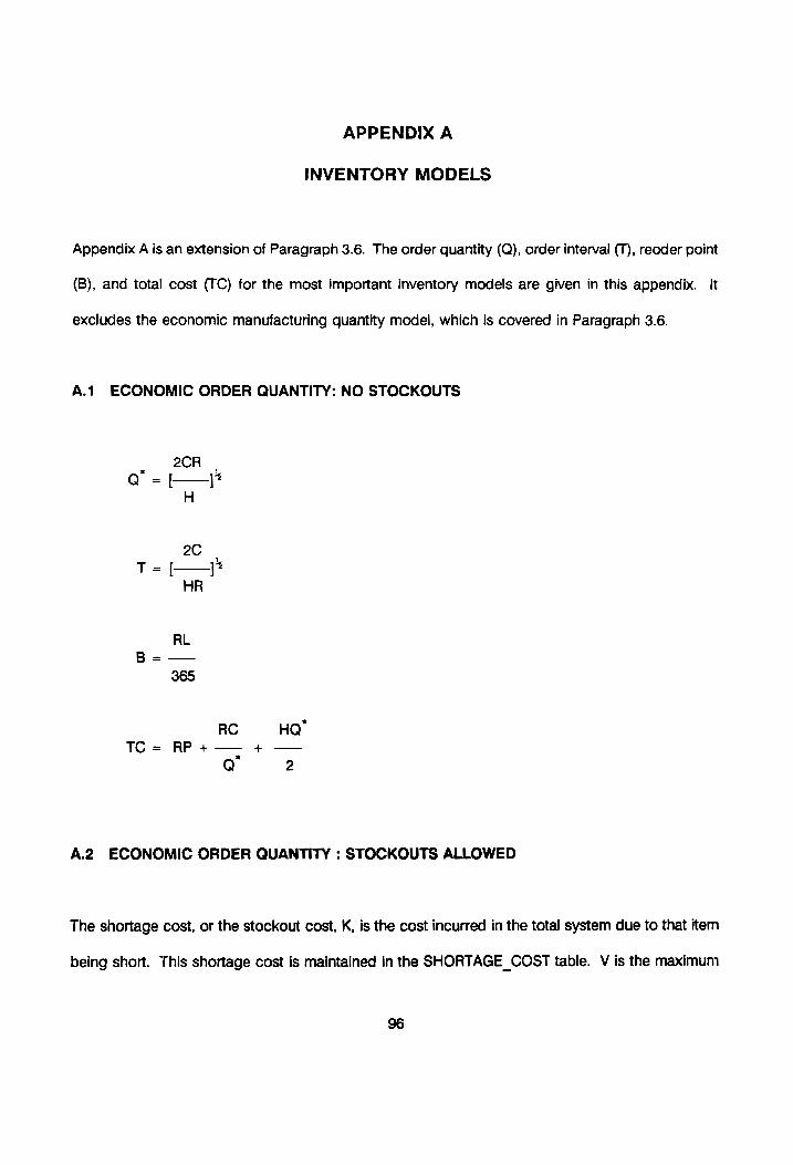
APPENDIX A
INVENTORY MODELS
Appendix A is an extension of Paragraph 3.6. The order quantity (Q), order interval (T), reoder point
(B), and total cost (TC) for the most important inventory models are given in this appendix. It
excludes the economic manufacturing quantity model, which is covered in Paragraph 3.6.
A.1 ECONOMIC ORDER QUANTITY: NO STOCKOUTS
“
RC HQ TC = RP +—— + —
Q 2
A.2) ECONOMIC ORDER QUANTITY : STOCKOUTS ALLOWED
The shortage cost, or the stockout cost, K, is the cost incurred in the total system due to that item
being short. This shortage cost is maintained in the SHORTAGE_COST table. V is the maximum
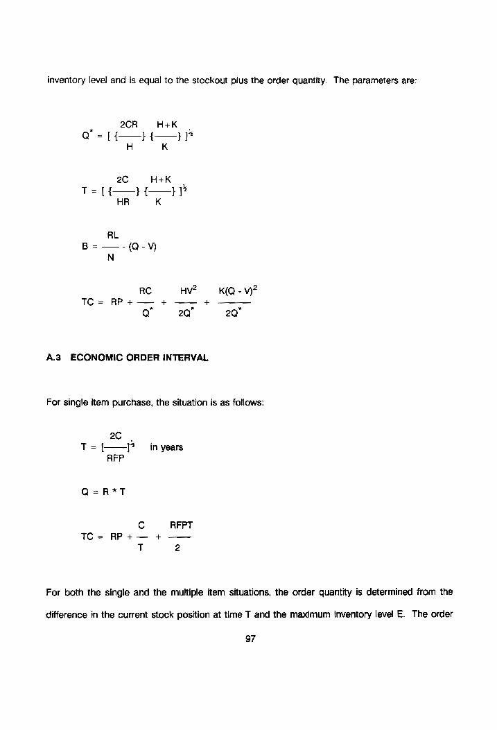
inventory level and is equal to the stockout plus the order quantity. The parameters are:
. 2CR H+K
Q =[{i—}f{ } }? H K
2C H+K
T= [{—}{ +}? HR K
RL =—-(Q-YV)
N
RC HV7—s_ K(Q.- V)? TC = RP +— + - + -
Q 2Q 20
A.3) ECONOMIC ORDER INTERVAL
For single item purchase, the situation is as follows:
2c | T=[ ]? in years
RFP
Q=R*T
C RFPT TC = RP +— +
T 2
For both the single and the multiple item situations, the order quantity is determined from the
difference in the current stock position at time T and the maximum inventory level E. The order
97

quantity averages out as RT. The reorder point B is not very important since orders are made
periodically. The maximum inventory level E is:
R*(T +L)
N
Q+8
Both T and L are expressed in days. For the multiple item purchase, there is an extra ordering cost
per order, Cc", (consisting of multiple items), apart from the individual! item ordering cost. The
EOI_MULTIPLE_ITEMS table indicates all the items that are procured together. The column MULT#
indicates the unique number that identifies the items that are ordered as a group: all items with the
same MULT# are procured together.
EOI MULTIPLE ITEM
ITEM# MULT#
SDF M45 GHI M45 OPQ J32 GGN M45 G54 J32
The EOI MULT COST table indicates the order cost, C”, per multiple item order in the ORD_COST
column.
EOI_MULT COST
ITEM# ORD_COST
M45 245.00
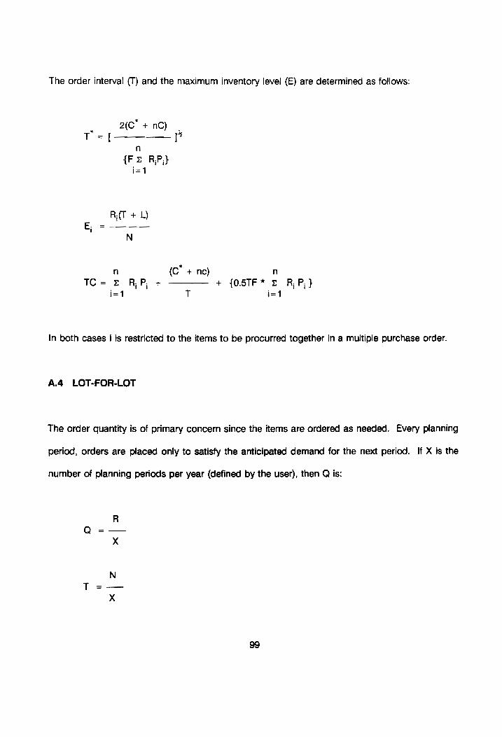
The order interval (T) and the maximum inventory level (E) are determined as follows:
2(C” + nC)
T = [——__}* n
{F = RP,} i=
R(T + L) E, =
N
n (C* + nc) n TC = = RP. + ———— + {05TF* & RP}
i=1 T i=1
In both cases i is restricted to the items to be procurred together in a multiple purchase order.
A.4_ LOT-FOR-LOT
The order quantity is of primary concern since the items are ordered as needed. Every planning
period, orders are placed only to satisfy the anticipated demand for the next period. If X is the
number of planning periods per year (defined by the user), then Q is:
R Q =—_—
X
N T=—
X

«x
HQ TC = RP + XC + ——
A5 PERIODIC ORDER QUANTITY
EOQ 20. T = EOl = = | ]?
Ravg RavgPt
EOI
i=1
X Q TC = RP + (— * C) + (C- * H)
T 2
r, is the average demand per period. The user is prompted to establish the length of a period
(days, weeks, months, etc.). These values are maintained in the PERIOD_LENGTH table. The
column PLAN_PERIOD is the planning period in days (D), weeks (W), months (M), or years (Y).
The periods are considered seven days per week, 30 days per month, and 365 days per year. The
value of X is selected accordingly, and the average demand per period is calculated, using the
number of hours per week, weeks per year, and the total number of days per year that the end user
wishes to work with the end item. If the system is being used constantly, r, is simply the average
demand per period (i.e., the total annual demand divided by the number of periods per year). The
holding cost fraction per period (f) is the annual holding cost fraction (F) divided by the number of
periods per year. The reorder point B is not of concern since the orders are placed with regular
intervals T. Ravg is the average demand rate over the entire planning horizon.
100

PERIOD_LENGTH
ITEM# PLAN PERIOD
KJH D GYK M KLP W
A.6 PART-PERIOD ALGORITHM
i ua oO
(k-1)R, = — 1 Ph
The order interval is determined by increasing k to the point where the left hand side of the above
equation exceeds the right hand side. R, is the demand rate during the k"" period. The reorder
point is, again, not of concern, but the order quantity is calculated from:
iM
=
1
X Q TC = RP + (— * C) + (C * H)
T 2
where the ratio X/T follows the same relationship as under the periodic order quantity. The
PEROID_LENGTH table is also used in determining the planning period length.
101

A.7 PROBABLISTIC: VARIABLE DEMAND & CONSTANT LT (K KNOWN)
The objective in the probablistic models is to determine the order size Q, the reorder point B, and
the safety stock, S. These parameters are all maintained in the INVENTORY table. The EOQ model
is used to determine the order size and is calculated and stored in the ORD_QUANT column of the
INVENTORY table (the variables are the same as discussed under the Economic Order Quantity):
The Poisson distribution is now used to determine the probability of a stockout during the lead time.
The lead time is taken from the LEAD_TIME column in the [TEM_PRICE table. Since lead time is
in working days, it has to be transformed in the following way to get the actual working time during
the lead time:
LT actual working time = t,7 = * (weeks/yr) * (hours/wk) 365
The (weeks/yr) and (hours/wk) terms are the total hours that the end user wishes to work during
a year and are retrieved from the tables CUSTOMER_WORKING WEEKS and
102

CUSTOMER WORKING HOURS respectively in the appropriate years. The failure rate ® (the
number of failures per hour) is a function of the annual failure rate in the TOTAL_FAILURES table.
The Poisson distribution can now be used to sequentially calculate the probability for the demand
of n (n = 0,1,2,...) spares during the lead time:
(® * t,)" * exp(-@ * t,7) , =n] = = P(M)
n!
P[D
where P(M) is the probability of having a lead time demand of M units. These probabilities are
significantly calculated to the third decima! point. These probabilities are sequentially added
together and subtracted from 1 until the optimum probability of a stockout is reached. The value
of n at that point is the reorder point B. It is calculated as follows:
n
P.” = P(M>B)=1- 2 P(M) i=0
The probability distribution of demand during lead time follows a Poisson distribution. P(M>B) is
the probability of the lead time demand being greater than the quantity at the reorder point B.
P(M>B) is, therefore, also equal to the probability of a stockout. These values are maintained in
the VARIABLE _DEMAND table. The columns are as follows: M is the lead time demand; P(M) is
the probability of having a lead time demand of M units; and P(M>B) is the probability of needing
more units during the lead time than the reorder quantity (which is also the probability of a
stockout).
103

VARIABLE_DEMAND
ITEM# M P(M) | P(M>B)
CVB 26 0.010 0.990 CVB 27 0.030 0.960 CVB 28 0.070 0.890
CVB 34 0.203 0.674 CVB 35 0.248 0.426 CVB 36 0.196 0.230
CVB “47 0.003 0.000 This table does not have to exist in reality since all the values can be computed from existing data
in other tables. Its existence, like in many other cases, would violate the concept of data
independence. On the other hand, its existence would ease the process of data configuration and
speed up queries. In the variable demand, variable lead time case, the assumption is made that this
table exists. If it doesn’t, the values will be calculated accordingly. The reorder point B is the value
of M that corresponds to the value of P(M>B) closest to Pp.” . The safety stock S is already built into
the definition of the reorder point and is equal to:
avg
where Mavg is the average demand during the lead time. This is equivalent to:
Mavg = @*tiy
RC Q" TC = RP +—— + (—— + S)*H
Q 2
104

The first time that the safety stock is acquired, this total cost formula changes to:
*
RC Q TC = (R + S)*P + — + (—— + S)*H
Q 2
A.8 PROBABLISTIC: VARIABLE LT & CONSTANT DEMAND (K KNOWN)
A probability distribution must be defined for the lead time. This distribution is maintained in the
table VARIABLE _LT. Contrary to the VARIABLE DEMAND table, the VARIABLE _LT table must exist
since, in this case, it contains raw data. The columns LT, PROB, and SUPPLIER are the lead times
and its associated probabilities of occurance, and the supplier of each item. The lead time in this
table is for the exclusive use of the probablistic approach to a constant demand, variable lead time
supply situation and does not replace deterministic values of the LEAD TIME column in the
ITEM_PRICE table. An item cannot have a constant lead time in the ITEM_PRICE table as well as
a lead time probability distribution in the VARIABLE _LT table; it must have one or the other. The
ITEM_PRICE table shows blank values for the lead time if it has a probability distribution, and the
user is pointed towards this distribution when the field is queried. For each item and supplier, the
probabilities must sum to one.
VARIABLE LT
ITEM# SUPPLIER LT PROB
XDF S05 10 0.15 XDF sos 11 0.20 XDF S05 12 0.25 XDF sos 13 0.20 XDF Sos 14 0.15 XDF S05 15 0.05
105

The constant demand on a daily basis (LT is in calendar days) is multiplied by the different lead
times to obtain the actual lead time demand M corresponding to the probability of occurence. M
still corresponds to the probability distribution. Since the demand is constant and the lead time
varies, a probability distribution is obtained from the different lead time demands. The table
VARIABLE DEMAND can also be used to save the results of this process. (The table
INV_ITEM_ MODEL keeps track of the fact that this is a constant demand, variable lead time case.)
The average lead time demand M,,, is calculated as:
Mayg = = M * P(M)
The summation is for all the probabilities and their associated lead time demand. The reorder point
B is further calculated in the same way as in the constant demand, variable lead time case. The
safety stock is then calculated as the difference between the newly calculated reorder point B and
actual average demand M,,,. The total cost is then:
*
RC Q TC = RP +—— + (—— + S)*H
Q 2
The first time that the safety stock is acquired, this total cost formula changes to
*
RC Q TC = (R + S)*P +—— + (—+S)*H
Q 2
106

A.9 PROBABLISTIC: VARIABLE DEMAND & VARIABLE LT (K KNOWN)
Both the VARIABLE DEMAND and the VARIABLE _LT tables are utilized in this case. The standard
deviation of the demand distribution, cp , and the standard deviation of the lead time distribution,
o, , must be calculated from the tables VARIABLE DEMAND and VARIABLE LT respectively. The
standard deviation of the lead time is calculated as follows:
n
= Freq, * (LT, - LTayg )?
a | 0.99 '
where Freq, is the probability of occurence in the VARIABLE_LT table. LT; is the i” lead time that
corresponds to Freq, . LT avg is simply the summation of the product of LT; and Freq; for all the
values of i. The standard deviation of the demand distribution is obtained in a similar fashion. In
the case where the lead time and the demand distributions are independent, the variance of the
demand during the lead time, o7 , can now be calculated as:
2 2 o = (LTayg * Op-) + avg * 9,7)
where Dayg is the average demand during the lead time, calculated in a similar way as LT... For
the case where the demand and the lead time are dependent on each other, the variance will be
calculated as:
a = {(LT ay)? * op } + {(Dayg)* * 9:7} + {op * o}
107

For both the independent and dependent cases, the mean of the demand during the lead time is
approximated by M,,, :
avg ~ “avg avg
Since the mean and variance are known, and assuming a normal distribution, the reorder point B
can now be expressed as:
The value of Z corresponds to the desired probability of having a spare part available upon request
(from normal distribution tables). The safety stock S is calculated from:
x
RC Q TC = RP +-— + (—— + S)*H
Q 2
The first time that the safety stock is acquired, this total cost formula changes to.
=
RC Q TC = (R + S)*P + — + (—— + S)*H
Q 2
108

A.10 PROBABLISTIC: STOCKOUT COSTS UNKNOWN
When stockout costs can not be determined with a reasonable amount of certainty or when
management does not want to take the risk of estimating it, a service level can be specified. This
service level is simply the probability of having a spare part available upon request, P..,;. A
probability value is specified (typically 0.97) and the number of spares is then calculated, using the
Poisson distribution. This value is the reorder point, B. The order quantity is stil! the Economic
Order Quantity. Again, only the lead time is of concern. P,,,; is then calculated as:
B (@ * t,,)" * exp(-@ * t.;) P x avail —
n=0 n!
The safety stock is the difference between the reorder point and the average lead time demand
(®*t, +). The inventory table is updated accordingly. The total cost is:
*
RC Q TC = RP +-— + (—+S)*H
Q 2
The first time that the safety stock is acquired, this total cost formula changes to:
*«
RC Q TC = (R + S)*P + —— + (-—— + S)*H
Q 2
109

APPENDIX B
INTERFACE WITH MANUFACTURING PLANNING AND CONTROL
There is an important interface between the proposed model (as a result of this research) and
Manufacturing Planning and Control (MPC). This interface results primarily from the fact that MPC
use a fair amount of data that have already been accumulated by the application of the proposed
model in the earlier phases of design. Using these data will give MPC a “running start."
MPC also utilizes the concept of product structure, or bill of material. In fact, the product structure
is the backbone of MPC. All the important data and functions of MPC are linked together by means
of the product structure: production schedules, capacity planning, inventory control, purchasing,
and others. The most basic input to MPC is the product structure. The most important output as
a result of this research is the product structure; the configuration that will fulfill all the customer
requirements at a minimum life-cycle cost. MPC deals with all the activities in a manufacturing
context from acquisition of raw materials to delivery of completed products. As the name implies,
the purpose of MPC is to plan and control manufacturing activities. MPC neither looks at the design
and development phases of a system, nor does it look at the utilization and support phase, other
than having bills of material as references. The other important output of the proposed model is
the definition of the logistic requirements to effectively support the system throughout its utilization
phase. Because the proposed model covers the entire life cycle of a system, and because it utilizes
a good portion of the data that are required by MPC (as will be outlined in the rest of Appendix B),
there must be an important interface between the proposed model and MPC.
An ideal is to integrate the proposed model and MPC to have a firm control on the product
110

throughout its life cycle. Such an integrated system will have the following capabilities:
1. The product configuration that will be selected will fulfill the requirements of the end user
at a close-to-minimum cost.
2. All important aspects of production will be planned immediately for the selected
configuration. This includes production scheduling, material planning, inventory control,
cost accounting, budgeting, capital budgeting, resource and capacity requirements, and
purchasing. A large percentage of the data that were used to determine the preferred
product configuration will be used in MPC.
3. The logistic requirements for the preferred configuration will be determined.
In such an integrated system these capabilities will be interactive: whenever a change in one aspect
occurs, the others will be updated accordingly. Eg., when the cost of a maintenance activity for a
certain item exceeds a certain limit, another design configuration can be proposed with a detail
breakdown of the impact on the system (including cost): new production schedules, new
manufacturing and maintenance processes, new material planning, training requirements, resource,
Capacity, and manpower requirements for manufacturing and support, inventory requirements for
manufacturing and for the customer, and more.
The rest of Appendix B is devoted to briefly describing MPC and its interfaces with the proposed
model. Figure 6 illustrates the main elements of MPC. The top part, or the front end (FE), is the
set of activities and systems for overall direction setting. The front end is used to establish the
company objectives for MPC. The middle part, or engine (ENG), is the detailed planning of material
111

flow and capacity to support the overall plans. The bottom part, the back end (BE), is the execution
of the plans, as generated in the engine, in terms of detailed shop scheduling and purchasing
actions. Each of the MPC activities outlined in Figure 6 are described in the subsequent
paragraphs. The interfaces with the model are also indicated.
RESOURCE PRODUCTION DEMAND PLANNING PLANNING MANAGEMENT
ROUGH-CUT MASTER CAPACITY PRODUCTION PLANNING SCHEDULING
oO")
FE
DETAILED MATERIAL INVENTORY CAPACITY REQUIREMENTS CONTROL PLANNING PLANNING
ENG
SHOP-FLOOR PURCHASING CONTROL
BE
Figure 6 Main elements of MPC
112

B.1 PRODUCTION PLAN
The production plan provides the key communication (in the form of direct and consistent dialogue)
from top management to manufacturing and is derived from, and is consistent with, the strategic
plan of the company. It determines the basis for focusing the detailed production resources to
achieve the strategic objectives of the firm. The production plan states the mission that
manufacturing must accomplish if the overall objectives of the firm are to be met. The production
plan is stated in terms of monthly or quarterly sales dollar output (for the company as a whole, or
for the individual business units), or in terms of number of units to be produced in each major
product line for the next month, quarter or year. How the production plan is to be accomplished
in terms of detailed manufacturing and procurement decisions is a problem for manufacturing
management. With an agreed-upon game plan, the job of manufacturing is to "hit the production
plan." Also, the production plan provides the basis for monitoring and controlling manufacturing
performance in a way that provides a much clearer division of responsibilities than is true under
conventional budgetary controls.
The production plan is the actual number of units that must be deployed in order to fulfill the user's
requirements. This information is received from the UNITS DEPLOYED table (column TH_PRAC
= "P"). This table contains the number of units that must be delivered each year. Manufacturing
must add together all the identical items, regardless of where each unit is deployed (LOCATN).
B.2} DEMAND MANAGEMENT IN MPC
Demand management links the marketplace with manufacturing planning and control. It is through
demand management that a channel of communication is maintained between the MPC systems
113

and their "customers." Demand management encompasses forecasting, order entry, order-delivery-
date promising, customer order service, physical distribution, and other customer-contact-related
activities. Demand management is also concerned with other sources of demand for manufacturing
capacity. Included are service-part demands, intracompany requirements, and pipeline inventory
stocking. All quantities and timing for demands must be planned and controlled. A primary function
of the demand management module is to convert specific day-to-day customer orders into detailed
MPC actions. It is through the demand management function that the actual demands consume
the planned materials and capacities. Demand management is accomplished by assuring that all
the user functional requirements are correctly interpreted. The following tables are the responsibility
of those in charge of demand management:
1. DETAIL_REQUIREMENTS
2. TOTAL_REQUIREMENTS
3. CUSTOMER WORKING HOURS
4. CUSTOMER WORKING WEEKS
5. CAPACITY_DESCRIPTION
B.3 MASTER PRODUCTION SCHEDULING
The master production schedule (MPS) is an anticipated build schedule for manufacturing end
products. It is primarily derived from the production plan, with inputs from market demand and
rough-cut capacity planning. As such, it is a statement of production and not a statement of market
demand. That is, the MPS in itself is not a forecast. An effective MPS provides the basis for:
1. Making customer delivery promises.
114
2. Utilizing the capacity of the plant effectively.
3. Obtaining the strategic objectives of the firm as reflected in the production plan.
4. Resolving trade-offs between manufacturing and marketing.
The MPS forms the basic communication link with manufacturing. The MPS is stated in part
numbers for which bills of materials exist. It cannot be stated in dollar value. The specific products
in the MPS can be end-item designations (i.e., complete assemblies or spare parts) or it can be
groups of items such as models instead of end-items. The MPS must be stated in such a way that
the number of units to be deployed match the values in the UNITS DEPLOYED table.
B.4 MATERIAL REQUIREMENTS PLANNING
Materia! requirements planning (MRP) is the central activity in manufacturing planning and control
(MPC). The managerial objective of MRP is to provide the right part at the right time to meet the
schedules for the completed products. An MRP system ensures that planning is integrated, that is,
that the correct number of components and raw material for each component is planned for each
end product. A bill of material, or product structure, must exist. Most of this data is received from
the following tables:
1. PRODUCT STRUCTURE
2. ITEM_IDENTIFICATION
3. ITEM PRICE
4. COMMODITY
115

Obviously, these tables have data only to the level relevant (or known) during the early stages of
design. The data from these tables must be expanded to include the lowest level that requires
planning. However, these tables serve not only as an initial source of data, but also as a baseline.
All lower level data must add up to the values in these tables. If not, replanning or redesign is
required.
MRP takes a period-by-period, or time-phased, set of a master production schedule and produces
a resultant time-phased set of component or raw material requirements. Practically, this means that
MRP breaks down each requirement in the MPS to the point where it suggests exactly when each
raw material part is to be procured (considering lead times, safety stock and re-order quantities).
It also prescribes when components should be released to be manufactured or assembled into
higher level assemblies. It therefore acts as a translator of the overall plans for production into the
detailed individual steps necessary to accomplish those plans. The bill of material (or product
structure) serves as a primary input to the material requirement planning activity.
B.5 CAPACITY PLANNING
In order to fulfill a market demand the company must have the necessary resources with sufficient
Capacity. The objective of capacity planning is to ensure that sufficient capacity is available to
accomplish the planned production in order to fulfill the market demand. The benefits of an effective
MPC system can only be fully realized with the provision of adequate capacity; too little or too much
Capacity can be harmful. There are basically four levels in capacity planning:
The Resource planning activity is directly linked to the production planning module. It is the most
highly aggregated and jiongest-range capacity planning decision. Resource planning typically
116

involves converting monthly, quarterly, or even annual data from the production plan into aggregate
resources such as gross labor-hours, floor space, machine-hours, and the like. This level of
planning involves new capital expansion, which requires a time horizon of months or years.
Rough-cut capacity planning has the master production schedule as its primary source of
information. The capacity requirements of a particular master schedule can be estimated by any
of the following techniques: capacity planning using 1) overall planning factors (CPOF), 2) capacity
bills, or 3) resource profiles. These techniques provide information with which to modify the
resource levels or material plan in the medium range to ensure efficient execution of the master
production schedule.
The Capacity Requirements Planning (CRP) is used for detailed capacity planning. The material
plans produced by the MRP system serve as the basis for calculating time-phased capacity
requirements. The data files used by the CRP technique include work in process, routing,
scheduled receipts, and planned orders. The information provided by the CRP technique can be
used to determine the short-term capacity needs for both key machine centers and labor skills.
The types of facilities, tools, and labor required to perform manufacturing activities will most
probably be the same as those required for logistic repair activities. The unit capacities of each of
these elements, as well as the frequency of use, must be considered in estimating the capacity for
the manufacturing activity. Costs are estimated accordingly. The following tables provide essential
data:
1. GENERAL_FACILITIES
2. FACILITIES
117

3. GENERAL TOOLS
4. TOOLS
5. GENERAL_TRAINING
6. TRAINING
7. GENERAL_PERSONNEL
8. ITEM_PERSONNEL
9. CORREC_MAINT LABOR
10. CORRECT PERSONNEL
11. PREVENT MAINT LABOR
12. PREVENT PERSONNEL and UNIT_PACKAGE
B.6 INVENTORY
In a production control environment, the primary functions of inventory control are the following:
1. To ensure that the production function is not hampered by lack of required items, or a
surplus of them.
2. Minimum cost is expended on the inventory function, provided production is commensurate
within acceptable component availability.
Only the inventory at the manufacturing facility is of concern. Determining of desired inventory
levels and maintaining inventory at these levels are the heart of the inventory control problem. Lot
sizing, order quantities and reorder points are determined for all types of inventory. These types
of inventory usually consist of supplies, raw materials, in-process goods, and finished goods.
118

Supplies are inventory items consumed in the normal functioning of an organization that are not a
part of the final product. Typical supplies are pencils, paper, light bulbs, typewriter ribbons, and
facility maintenance items. (Factory supplies are called MRO; standing for maintenance, repair, and
operating supplies.) Raw materials are items purchased from suppliers to be used as input into the
production process. They will be modified or transformed into finished goods. Typical raw
materials for a furniture manufacturer are lumber, stain, glue, screws, nails, and varnish. In-process
goods are partially completed final products that are still in the production process. They represent
both the accumulation of partially completed work and the queue of material awaiting further
processing. Finished goods are the final product, available for sale, distribution, or storage.
Although inventory control is limited to the inventory function at the end-user (for the purposes of
this study), there must be some form of consistency in principles between the management of
inventory at the end-user and for that of manufacturing. Some comparisons can be made between
these two types of inventory.
B.7 SHOP FLOOR CONTROL
Shop Floor Control (SFC) manages the detailed flow of materials inside the plant. MRP provides
the materials plans that SFC executes: to build the right part at the right time. (The materials plan
is derived from MRP and sets performance objectives.) This will result in the ability to fulfill the
master production schedule and satisfy the production plan, while at the same time _ satisfy
customer service objectives.
MRP and capacity requirements planning (CRP) together produce capacity plans (what capacity
required from what work center, in what time). The capacity plan is especially critical to managing
119

the detailed shop floor flow of materials. In essence, the capacity provided represents the resource
availabilities for meeting the material plans.
Many of the logistic repair activities are approximately the same than the original manufacturing
activities. This means that the common information can be shared. Although the model (as a result
of this study) does not go down to the level required for shop floor control, many tables can help
assessing the required data.
B.8 PURCHASING
Purchasing is at the back end of the MPC system, and has the objective of executing the detailed
planning developed by the material and capacity planning techniques. The integration of MPC
systems with purchasing (and therefore the vendors) represents one part of an overall program to
improve supplier cost and quality performance. The object of the MPC system is to improve the
planning and control of vendor capabilities through procurement; thereafter, vendor capabilities are
scheduled in ways analogous to those used in shop-fioor control. The most important functions of
purchasing are (listed from strategic importance to the firm to immediate action activities that effect
day to day business): Sourcing, value analysis, contracting, budgeting, purchasing, and
monitoring.
Purchasing is a very low level activity and is only touched on during this study. The prices and lead
times for items needed for manufacturing should have a close relationship with the prices and lead
times promised to the customer in the ITEM PRICE table. There must be consistency between
these two values.
120
VITA
G. Chris Moolman was born on October 10, 1962 in Johannesburg, South Africa. He grew up
primarily in George, South Africa. After completing a Bachelor of Engineering in Mechanical
Engineering at the University of Stellenbosch in 1985, he spent two years as a design engineer in
the South African Air Force, achieving the rank of Lieutenant. Subsequently, he was employed as
a systems engineer for two years and also received a Master of Engineering in Industrial
Engineering at the University of Pretoria, South Africa, in 1989. He is married to the former Karin
Coetzee.
121
Related Documents