› recherches › VORTEX › publications › ... · Modeling 3D animals from a side-view sketchModeling 3D animals from a side-view sketch Even Entema,b, Loic Barthea, Marie-Paule

Modeling 3D animals from a side-view sketch

Even Entema,b, Loic Barthea, Marie-Paule Canib, Frederic Cordierc, Michiel van de Panned

aIRIT - University of ToulousebUniversity of Grenoble-Alpes, CNRS (Laboratoire Jean Kuntzmann) and Inria

cUniversity of Haute AlsacedUniversity of British Columbia

Abstract

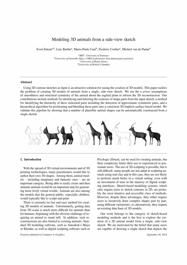
Using 2D contour sketches as input is an attractive solution for easing the creation of 3D models. This paper tacklesthe problem of creating 3D models of animals from a single, side-view sketch. We use the a priori assumptionsof smoothness and structural symmetry of the animal about the sagittal plane to inform the 3D reconstruction. Ourcontributions include methods for identifying and inferring the contours of shape parts from the input sketch, a methodfor identifying the hierarchy of these structural parts including the detection of approximate symmetric pairs, and ahierarchical algorithm for positioning and blending these parts into a consistent 3D implicit-surface-based model. Wevalidate this pipeline by showing that a number of plausible animal shapes can be automatically constructed from asingle sketch.

1. Introduction

With the spread of 3D virtual environments and of 3Dprinting technologies, many practitioners would like toauthor their own 3D shapes. Among them, animal mod-els – including imaginary and fantastic ones – are animportant category. Being able to easily create and thenanimate animals would be an important step for generat-ing more lively virtual worlds. Animals are also amongthe models that the general public, especially children,would typically like to sculpt and print.

There is currently no fast and easy method for creat-ing 3D models of animals. Unfortunately, getting datafrom 3D scans is much more difficult for animals thanfor humans, beginning with the obvious challenge of re-quiring an animal to stand still. In addition, such re-constructions are also limited to existing animals. Stan-dard 3D modeling software, such as Autodesk’s Mayaor Blender, as well as digital sculpting software such as

Pixologic-Zbrush, can be used for creating animals, buttheir complexity limits their use to experienced or pas-sionate users. The use of 3D sculpting is possible, but isstill difficult: many people are not adept at sculpting an-imals using real clay and in this case, they are not likelyto perform much better in a virtual setting, even withan investment of time in the mastery of digital sculpt-ing interfaces. Sketch-based modeling systems, whichonly require users to sketch contours in 2D, are proba-bly the most intuitive and accessible class of methods.However, despite these advantages, they either requireusers to iteratively draw complex shapes part by part,using different viewpoints, or, alternatively, they requirean existing data-base of 3D models.

Our work belongs to the category of sketch-basedmodeling methods and is the first to explore the cre-ation of a 3D animal model from a single, side-viewsketch. We are motivated by the belief that many usersare capable of drawing a single sketch that depicts the

Preprint submitted to Computer & Graphics September 30, 2014

contour lines and the internal silhouettes of an animal,such as shown in the top-left of Figure 1. If needed,users can use a background drawing or a photo as aguide. The process of inferring 3D geometry from the2D sketch necessitates the use of relevant assumptionsin order to be tractable, and in our context of modelinganimal forms, we shall assume smoothness of the result-ing shape as well as the presence of structural symme-tries. Several further moderate constraints include: (a)restricting ourself to non self-overlapping limbs in thesketch; (b) requiring the user to draw both contours forpairs of symmetric limbs; and (c) ignoring the recon-struction of repetitive details scattered on the surface,such as scales. With these assumptions and constraintsin place, the method we develop is capable of automat-ically converting an input vectorized sketch into a 3Dmodel. The total processing time is less than one sec-ond, effectively enabling one to create new animal mod-els in only the time required to sketch them.

Note that in this work, we only tackle the creationof the volumetric shape parts of an animal and that wedo not consider the surface components that should beused for ears or scales. The ears we reconstruct arealso therefore interpreted as volumes. We are not ableto reconstruct large flat parts such as wings. In addi-tion, we reconstruct limbs in a symmetric fashion, evenwhen they were drawn in arbitrary postures in the inputsketch. The construction of symmetric 3D models isusually desirable, as it ensures that left and right limbshave identical dimensions. To achieve a desired non-symmetric posture, the 3D model can be deformed, ei-ther by using an animation skeleton and the associatedskinning weights, or by directly articulating the implicitsurface’s skeleton.

Our processing pipeline for creating 3D animals froma sketch is summarized in Section 3. It consists of threemain steps, which also correspond to our three technicalcontributions:

1. the identification of the animal’s foreground struc-tural parts in the sketch, with completion of theparts that are not explicitly bounded, such as thetop of the legs (see the teaser figure)

2. the generation of a hierarchical graph of depths forthe structural parts, using the complete results andbased on an algorithm for detecting the portions ofthe sketch that correspond to symmetrical parts ofthe animal;

3. 3D reconstruction based on a specific choice ofimplicit surface, scale invariant integral surfaces,which enables us to accurately reconstruct shapeparts from their medial axis in the 2D sketch,

and to seamlessly blend them into a single animalmodel.

2. Related Work

2D sketches only represent the contours, silhouettesand main features of an object. Converting them intoa 3D model therefore requires resolving indetermina-cies and inferring a large amount of missing data. Fourstrategies are commonly used to do so, each of whichis based on a different level of hypotheses or a prioriknowledge of the shape being modeled (see [1] and [2]for detailed surveys):

Iterative methods enable the user to build general mod-els part by part, by iteratively adding new shape com-ponents from different viewpoints, e.g. the Teddy sys-tem [3]. These methods make the hypothesis that thefinal shape is a combination of parts that all have planarsilhouettes from a given viewpoint, and can therefore beinflated from closed planar contours. Animals belong tothis category but in practice these methods still requirepractice and time in order to achieving a convincing re-sult. Other iterative methods have been developed us-ing alternatives to inflation for geometric construction.These include the use of primitives such as generalizedcylinders and ellipsoids, as in [4], and methods basedon implicit surfaces, as in [5] or [6].

Shape matching approaches match the user sketchwith silhouettes, or parts of silhouettes of predefined3D models, possibly enabling some deformation. Thismethod was successfully applied to organic shapes suchas humans or animals [7], as well as for technical mod-els [8]. However, they require a template example of thegiven general class of animal which imposes a restric-tion on the family of sketches that can be used. We didnot consider this approach in our case, in order to allowthe user to imagine any animal shape without furtherrestrictions on the number of limbs, horns, etc.

Multi-view methods, e.g., [9], generate 3D shapesfrom two or three sketches drawn from orthogonal view-points. They require the ability to draw consistent viewsof the shape to be reconstructed. They are thereforemore easily applicable to man-made objects than to or-ganic shapes. Alternatively, a number of man-made ob-jects can be easily built from a network of 3D curves,which can themselves be directly reconstructed fromperspective sketches [10, 11]. However, these methodsrequire more user input than a single contour sketch,and are generally difficult to apply to the modeling offree form, organic shapes.

2

a) b) c) d)

e) f) g) h)

i) j) k) l)

z0

Figure 1: Overview of algorithmic stages: a) Half-edge graph; b) Detailed view of the resulting bounded curves; c) Cycles extracted from thegraph, each one depicted in a different color; d) Classification of cycles: the different colors now represent the cycle type; e) Detection of suggestivecontours; f) Completion of contours around shape parts; g) Detection of the main body and of pairs of symmetrical parts (displayed using the samecolor); h) Extracting a depth ordering; i) Skeletons extracted from the medial axes of shape parts; j) Reconstructed shape parts; k) Front view:inferring depth information for shape parts; l) Final result after implicit blending.

Lastly, direct methods try to infer 3D shapes from asingle complex sketch that depicts complex silhouetteswith loops, branches, cusps and T-junctions [12]. Thistechnique is probably the most appealing, since it im-poses few restrictions on the sketch being drawn, andmimics the human ability to see in 3D when provideda single, 2D-only representation. Different levels ofa priori knowledge are used for performing this task,spanning the range from very specific context based hy-potheses, as in methods for sketching flowers [13], gar-ments [14], trees [15] or blood vessels [16] to more gen-eral methods, such as the one for reconstructing arbi-trary shapes under the hypothesis of exact geometricalsymmetry [17]. Our research belongs to this last cat-egory. In the context of working with animal shapes,

we leverage the hypotheses of symmetrical subshapeswith planar contours, smoothly blending with the mainbody. In contrast to related prior work exploiting sym-metry [17], we do not demand exact geometrical sym-metry to be present in the input sketch, which would bedifficult to draw for most users.

3. Overview

Our method builds a 3D model from a single 2Dsketch. This involves the following steps, which are alsosummarized in Figure 1.

We start from a sagittal-view vectorized sketch of ananimal in the (x, y) plane. The hand-drawn input sketchis transformed into a set of parametric curves using a

3

(a) (b)

Figure 2: Two cases of failure: (a) Discontinuous sketch: a large discontinuity, as the one on the left, prevents the detection of the main body part inthe drawing. In that case our algorithm fails from its first steps. A small gap in the sketch, as on the left, is filtered and considered as a connectionduring our first step. The reconstruction will perform adequately. (b) Incomplete sketch: on the left, a structural part is missing in the sketch, here,the left inner-body silhouette of the front foreground leg. Our algorithm will not be able to detect the presence of a limb and the reconstructionof the legs will fail. On the right, both inner-body silhouettes of the rear foreground leg are drawn and the rear legs will therefore be adequatelyreconstructed.

vectorization algorithm such as the one proposed byNoris et al. [18]. These algorithms are relatively robustto noise and provide the smooth curves we seek. Whatthe user must really pay attention to is the correctness ofthe input hand-drawn sketch topology, i.e., the provisionof continuous closed contours that do not have spuriouscrossings with other contours. Figure 2 illustrates twofailure cases, the first, in 2(a), is due to an incorrectlyclosed contour and the second, in 2(b), is due to an in-complete input.

The goal of the first step, detailed in Section 4, is toidentify the strokes that correspond to the same struc-tural part, such as an eye, leg, or body, and to infer anymissing curves, i.e., perform contour completion, if theresulting contour is open. This is done in the followingway: We build a counter-clock-wise oriented half-edgegraph whose edges are in general bounded parametriccurves (see Figure 1(a,b)). In this graph, we iterativelyfollow successive half-edges, and store cycles in a list(Figure 1(c)). Each cycle is classified as being eitheran outer-sketch, island, border or other as explained inSection 4.1 and illustrated in Figure 1(d).

We then define as inner-edges those edges where bothhalf-edges belong to the same cycle (the green edges inFigure 1(e)). These lists of inner-edges represent sug-gestive curves where two shape parts merge (such as aleg merging with the body). This implies the presence ofhidden silhouettes or cusps [12]. Each suggestive curvehas an open endpoint and a closed endpoing, which aredepicted in red and blue, respectively, in Figure 1(e).The next step is to pair these suggestive curves and con-

nect their extremities in order to infer new cycles repre-senting the different structural parts of the animal (Fig-ure 1(f)). This is the topic of Section 4.2.

The subsequent step, presented in Section 5, is thecomputation of a depth hierarchy for structural parts,based on the structural symmetry hypothesis. We firstidentify the main body part located in the saggital plane,i.e., the torso, and detect structural symmetries around itsuch as pairs of ears or pairs of front legs, cf. Section 5.1and Figure 1(g)). We then use the pieces of informa-tion we already gathered, e.g., island cycles, structuralparts, chest, and symmetries, to define a depth hierarchybetween structural parts, as detailed in Section 5.2 andFigure 1(h).

This leads us to the last step, detailed in Section 6which consists of the 3D reconstruction of the animalmodel. For each pair of limbs, only the one in theforeground of the drawing is considered during the re-construction steps. The 3D reconstruction of the back-ground limbs are added at the end of the process by sym-metry. We choose implicit surfaces to represent shapeparts, in order to benefit from their blending capabili-ties. We first compute the medial axis [19] of each struc-tural part (Figure 1(i)). Medial axes are then filtered andspecifically simplified in order to be be used as skeletonsfor 3D implicit surface modeling (Section 6.1 and Fig-ure 1(j). Among the variety of existing implicit models,we use scale invariant integral surfaces (SCALIS) [20]to accurately reconstruct shape parts (Section 6.2). Fig-ure 1(j)) shows the 3D reconstruction of each structuralshape part in isolation. Structural parts without sym-

4

metries are placed in the sagittal plane of the model.The depth of the foreground structural parts is com-puted using the thickness of their 3D reconstruction andthe thickness of the part to which it is connected in thesagittal plane (Section 6.3 and Figure 1(k)). Symmetricbackground parts are then added to provide the final 3Dmodel (Figure 1(l)). The final shape is obtained using asimple sum to blend the fields from the different implicitprimitives.

The next sections give a detailed presentation of oursolutions at each stage of this process.

4. Structural parts identification and completion

4.1. Representing the sketch as a set of cyclesThe first step is to decompose the curves of the sketch

into a set of cycles. This decomposition is a preliminarystep towards identifying the different parts of the animaldrawn in the sketch. In particular, this step is requiredfor the hidden contour computation and the contour clo-sure, as described in Section 5.

The input data is a hand-drawn sketch composed ofa set of non-crossing curves that are connected to eachother (see Figure 1(a)). Each of these curves is repre-sented by a pair of directed half-edges1 of opposite di-rection (see Figure 1(b)). The curves of the sketch arethen represented using a graph whose edges are the half-edges of the curves and whose nodes are the points atwhich the curves are connected to each other. Next, wedecompose this graph into a set of cycles.

Formally, a cycle is defined as a closed sequenceof connected half-edges; each half-edge shares its end-points with at least two other half-edges. We require thehalf-edges that compose a cycle not to cross each other;we also require the cycles to be topologically equiva-lent to a disk. Therefore, a cycle divides the sketch intoan ”interior” region and an ”exterior” region. In orderto define the interior of a cycle, cycles and their asso-ciated half-edges are given a direction which is eitherclockwise or counter-clockwise; the interior of the re-gion bounded by a cycle lies on the left side of the di-rected half-edges that compose this cycle.

The first cycle that we identify is the one whichis composed of the half-edges located along the outerboundary of the sketch. This cycle is oriented clockwiseand is unbounded; it corresponds to the outer region ofthe sketch. We name this the outer sketch cycle. Next,we identify the border cycles which are cycles that have

1Note that each graph edge geometrically correspond to a fullcurve of the sketch.

Figure 3: Selecting the next half-edge. In (a), the selection of thenext half-edge (shown in green) for T-junctions is chosen such thatthe angle between the next half-edge and the preceding one (shown inred) is the smallest possible. In (b), the selection of the next half-edgefor cusps.

one or several half-edges belonging to the outer bound-ary of the sketch. All of these cycles are oriented in acounter-clockwise fashion. The process to construct aborder cycle is as follows: we first select a half edgewhich is located along the outer boundary of the sketchand which has not yet been associated to a cycle. Wenext find its endpoint by following its direction and se-lect the next half-edge. This next half-edge is chosensuch that its direction is the same as the previous half-edge and the clock-wise oriented angle between the twohalf-edges is the smallest possible, as illustrated in Fig-ure 3. The process of finding the next half-edge is iter-ated until we reach the first half-edge.

Finally, we identify the island cycles; island cyclesare single half-edges that correspond to a closed curvewith no self-intersection and which are not connectedto any other curves of the sketch. These island cyclesare also oriented counter-clockwise, meaning that theydo not represent a hole but rather a surface feature of theanimal (such as the eye of cat model shown in Figure 1).After processing all the cycles, there may remain somecycles that could not be classified as any of the threetypes (outer sketch cycles, border cycles and island cy-cles); we mark these cycles as others.

4.2. Contour completion

The goal is now to convert the set of cycles intoclosed contours associated to each structural part of theshape.

Once the graph cycles are classified as describedabove, we use the hypothesis that structural parts haveat least one edge in contact with the outer part of thesketch, and consider only the border cycles. In these cy-cles, we extract the sets of neighbor embedded edges,

5

a) b)

c)

β0

α00

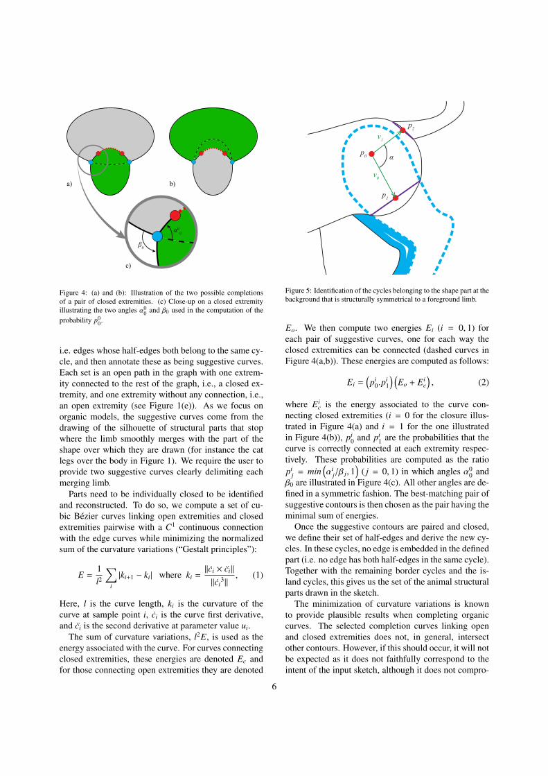
Figure 4: (a) and (b): Illustration of the two possible completionsof a pair of closed extremities. (c) Close-up on a closed extremityillustrating the two angles α0

0 and β0 used in the computation of theprobability p0

0.

i.e. edges whose half-edges both belong to the same cy-cle, and then annotate these as being suggestive curves.Each set is an open path in the graph with one extrem-ity connected to the rest of the graph, i.e., a closed ex-tremity, and one extremity without any connection, i.e.,an open extremity (see Figure 1(e)). As we focus onorganic models, the suggestive curves come from thedrawing of the silhouette of structural parts that stopwhere the limb smoothly merges with the part of theshape over which they are drawn (for instance the catlegs over the body in Figure 1). We require the user toprovide two suggestive curves clearly delimiting eachmerging limb.

Parts need to be individually closed to be identifiedand reconstructed. To do so, we compute a set of cu-bic Bezier curves linking open extremities and closedextremities pairwise with a C1 continuous connectionwith the edge curves while minimizing the normalizedsum of the curvature variations (“Gestalt principles”):

E =1l2

∑i

|ki+1 − ki| where ki =‖ci × ci‖

‖ci3‖

, (1)

Here, l is the curve length, ki is the curvature of thecurve at sample point i, ci is the curve first derivative,and ci is the second derivative at parameter value ui.

The sum of curvature variations, l2E, is used as theenergy associated with the curve. For curves connectingclosed extremities, these energies are denoted Ec andfor those connecting open extremities they are denoted

p0

p1

p2

v0

v1

α

Figure 5: Identification of the cycles belonging to the shape part at thebackground that is structurally symmetrical to a foreground limb.

Eo. We then compute two energies Ei (i = 0, 1) foreach pair of suggestive curves, one for each way theclosed extremities can be connected (dashed curves inFigure 4(a,b)). These energies are computed as follows:

Ei =(pi

0.pi1

) (Eo + Ei

c

), (2)

where Eic is the energy associated to the curve con-

necting closed extremities (i = 0 for the closure illus-trated in Figure 4(a) and i = 1 for the one illustratedin Figure 4(b)), pi

0 and pi1 are the probabilities that the

curve is correctly connected at each extremity respec-tively. These probabilities are computed as the ratiopi

j = min(αi

j/β j, 1)

( j = 0, 1) in which angles α00 and

β0 are illustrated in Figure 4(c). All other angles are de-fined in a symmetric fashion. The best-matching pair ofsuggestive contours is then chosen as the pair having theminimal sum of energies.

Once the suggestive contours are paired and closed,we define their set of half-edges and derive the new cy-cles. In these cycles, no edge is embedded in the definedpart (i.e. no edge has both half-edges in the same cycle).Together with the remaining border cycles and the is-land cycles, this gives us the set of the animal structuralparts drawn in the sketch.

The minimization of curvature variations is knownto provide plausible results when completing organiccurves. The selected completion curves linking openand closed extremities does not, in general, intersectother contours. However, if this should occur, it will notbe expected as it does not faithfully correspond to theintent of the input sketch, although it does not compro-

6

mise the rest of the reconstruction. If necessary, the usercan correct the completion by editing the extremities.

5. Depth hierarchy of structural parts

5.1. Body and symmetrical parts

In order to assign appropriate depth values, we createa graph that represents the desired depth relations. Thisbegins with the choice of a reference part as the rootnode of the graph, for which it is natural to use the bodyor torso. For some animals, this main body part maybe smaller than the limbs. As such, we did not find arobust method to automatically label this in the inputsketch. Instead, we request the user to select it or todraw the sketch so as to locate it in the center of thedrawing canvas. Once labeled, this part defines the nodeof reference for the graph. The method described belowautomatically locates the remaining structural parts withrespect to the body, in terms of their relative depth. Webegin by detecting the sketch strokes that correspond topairs of symmetric parts, as explained next.

We already know the parts, Fi, that should be locatedin front of the body and thus that may have a symmet-rical part in the background. These are defined by theopen contours with suggestive curves we just completedat the previous step. The goal is now to identify thestrokes from the sketch corresponding to Bi, the struc-turally symmetric part with respect to Fi, but located inthe background. Indeed, Bi should not be processed anyfurther, since we are going to use symmetric geometryto create the background limbs. In practice, Bi may becomposed of several distinct cycles, since it is partly oc-cluded. We use a propagation method for fully selectingit, as we now describe.

We initialize Bi with all cycles not belonging to theshape part under Fi, but that share an edge with Fi.We then compute the medial axis of Fi as described inSection 6. Let us denote as p0 the medial axis extrem-ity corresponding to the suggestive silhouette we closed(see Figure 5). We then denote as p1 the middle of theclosed extremities of the suggestive curves and then de-fine v0 = p1 − p0. Starting from both closed extremi-ties, we march along both sides (one clock-wise and theother counter-clock wise) of the cycle of the structuralpart which is located under Fi in the sketch, as long asthe opposite half-edge belongs to the outside sketch. Ifwe meet an opposite half-edge belonging to a border cy-cle, we get both extremities of the shared edge and wecompute their middle point p2. We define v1 = p2 − p0and compute the angle α = |v0, v1|. If α < π/4 we con-sider that this cycle potentially belongs to Bi, since the

angle formed by two symmetrical parts is unlikely to belarger than this value in usual standing poses. Note thatthis criterion could be relaxed to handle a larger set ofposes.

We stop when the half-edge we reach is an occludededge, i.e., when we meet the next foreground part. Ifselected on multiple occasions, a potentially symmetriccycle is assigned to the Bi for which the angle α withFi is minimal. The results of this selection process aredepicted in Figure 1(g), where pairs of symmetric partsare depicted using the same colors.

5.2. Graph construction

In order to support the 3D reconstruction of themodel, we build a graph whose nodes are the structuralparts (and their associated cycle) and whose edges rep-resent the relations over, under, adjacent or over-in withrespect to the main body. Foreground parts are definedas lying over the part they have been separated from.Symmetric counterparts are located under the part thattheir foreground is over. All remaining border parts thathave not been designated as part of a symmetric pair aredefined as being adjacent to parts with which they sharean edge. Islands are assigned to the graph by first usinga simple 2D ray-cast in the sketch plane in order to iden-tify the part within which the island lies. The island cy-cles are over and inside a structural part, and this part isalso then defined as being under the island. Each edge isfurther tagged with additional information, such as thepresence of suggestive curves, which help determine ifthe region being over a particular part is an island or alimb.

6. 3D Reconstruction

6.1. Medial-axis computation & simplification

Animals have the convenient property that their shapeis naturally approximated as a set of generalized cylin-ders. A generalized cylinder is a surface obtained bymoving a circle of varying radius along a 3D arbitrarycurve. An advantage of generalized cylinders is thattheir skeleton and associated radii are easily determinedfrom their projected image. Given a 2D simple closedcurve C, the skeleton and the associated radii of the gen-eralized cylinder whose orthogonal projection matchesC are obtained by computing the medial axis and theassociated radius function of the curve C.

We start the 3D reconstruction step by reconstruct-ing each structural part independently. The parts whichwere detected as being symmetric to foreground partsare not considered. The contour curve of each part is

7

a)

b)

Figure 6: Medial axis computation and simplication. In (a), the medialaxes of the sketch components computed using Fortune’s sweep-linealgorithm [19]. In (b), the skeletons after removing the branches usingthe Scale-Axis Transform [21] and after simplifying the medial axesusing the Douglas-Peucker algorithm [22].

first sampled so as to obtain a polygonal curve. Wethen compute the medial axis transform of each of thepolygonal curves using the Fortune’s sweep-line algo-rithm [19]. The medial axes usually contain manybranches because of the noise in the polygonal curves.We use the Scale-Axis Transform method by Giesen etal. [21] to remove these branches. In our experiments,the scale factor of the Scale Axis Transform has beenset to 1.2.

The last step is to simplify the medial axis; the pur-pose of this simplification is to lower the computationtime for generating the surface of the reconstructed an-imal. We have implemented a modified version of theDouglas-Peucker algorithm [22] which is a method toreduce the number of points of polygonal curves. Acost function is defined for each point, which is themaximum distance between the original curve and thecurve after removing the point. Points are removed iter-atively in increasing order of their cost. The algorithmstops when the cost of the point to remove is above a

user threshold. Figure 6(b) illustrate the result of the catskeletons simplification.

(a)

Ap

Bp Cp

(b)

d

Ap

Cp

Figure 7: Medial axis simplification. In (a), the polygonal curve (de-picted in black) and its medial axis (depicted in red) before the simpli-fication. In (b), the medial axis has been simplified by removing thepoint pB. The result is new polygonal curve with fewer segments. Thecost value of removing the point pB is d; it is the maximum distancebetween the original curve (depicted in light grey) and the curve afterthe simplification.

The Douglas-Peucker algorithm has been modified totake into account the radii of the medial axis. This mod-ification consists of a new cost function. Let C be apolygonal curve and pA, pB, pC be three neighboringpoints of the medial axis of C. If the point pB is re-moved, the two segments pA pB and pB pC are replacedwith the segment pA pC (see Figure 7). Similarly, thecurve corresponding to the medial axis is simplified;two of its segments are removed. The new cost func-tion is defined as the maximum distance d between theoriginal curve and the curve after the simplification ofthe medial axis.

6.2. Surface reconstruction of the shape componentsOnce the skeletons of all the shape components

have been computed, the next step is to reconstructthe 3D surface of these shape components. We haveimplemented the SCALe-invariant Integral Surfaces(SCALIS) method proposed by Zanni et al. [20]. Thismethod generates an implicit surface using a skeletonand its radius function. In Zanni’s method, the scalarfield is computed with the Homothetic Polynomial ker-nel of degree 8. In our method, we have implementedthe kernel of degree 6 instead of degree 8. Although thequality of the reconstructed surface is slighly lower, thecomputation time is much smaller, and allows for sur-face reconstruction at near-interactive rates. The result

8

IpA,0pA,1

a)

b)

I

pNA,0

r

Sket

chin

g p

lane

dA,1

dA,1

Sket

chin

g p

lane

Figure 8: Computation of the depth coordinates of the implicit surfaceIA. In (a), the depth coordinate dA,1 of the skeleton extremity pA iscomputed. In (b), the skeleton (depicted in red) of IA is translated tothe depth coordinate dA,1.

is a set of implicit surfaces, one for each shape compo-nent (see Figure 1(k)).

6.3. Placement & embedding of the shape components

The last step of the surface reconstruction is to as-semble the implicit surfaces to generate the 3D shapeof the animal. At this stage, the skeletons of the im-plicit surfaces are all located in the same plane whichis the sketching plane. The goal is to place these im-plicit surfaces so that their depth order complies withthat of the sketch; the shape components that are drawnin the sketch foreground should be placed in front ofthe sketching plane and those drawn in the sketch back-ground should be placed behind the sketching plane. Wemake use of the depth graph that has been previouslycomputed (see Section 5.2).

We start by placing the implicit surface correspond-ing to the main body component in the sketching plane.Other implicit surfaces are sequentially placed as fol-lows. Using the depth graph, we find a shape compo-nent that has not yet been placed and which is adjacentto a shape component which has already been placed.

Using the depth order between these two shape compo-nents, we compute the depth position of the one to beplaced.

Let IA and IB be two implicit surfaces, with IA beingin front of IB. The depth coordinates of IB have beenalready computed; those of IA have to be computed. LetpA and rA be the skeleton extremity of the implicit sur-face IA and its radius respectively. We first compute pA,0the orthogonal projection of pA onto IB. Next, we com-pute −−−→NA,0, the surface normal of the implicit surface IB

at the point pA,0. Finally, we compute pA,1 such that∥∥∥−−−−−−→pA,1 pA,0∥∥∥ is equal to rA and such that the two vectors

−−−→NA,0 and −−−−−−→pA,1 pA,0 are parallel and have same direction(see Figure 8(a)). The depth coordinate dA,1 of pA,1 isthen used as the depth coordinate of all the points of theskeleton of IA (see Figure 8(b)).

Once the depth coordinates of all the implicit surfaceshave been computed, the 3D shape of the animal is thengenerated by blending these implicit surfaces using thewell-known Ricci blending operator.

7. Results and discussion

Figure 9: Different views of the 3D reconstruction of the cat sketchedin the top-left.

We implement our method as a Maya plugin, en-abling us to use the existing sketching interface of Mayato design the vectorized sketches we need as input. Pro-cessing the 2D sketches into 3D models is then a fullyautomatic process.

9

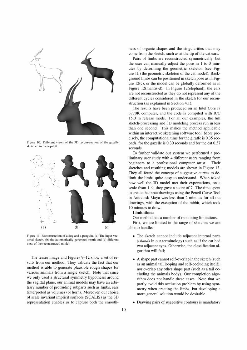
Figure 10: Different views of the 3D reconstruction of the gazellesketched in the top-left.

(a) (b) (c)

Figure 11: Reconstruction of a dog and a penguin. (a) The input vec-torial sketch, (b) the automatically generated result and (c) differentview of the reconstructed model.

The teaser image and Figures 9–12 show a set of re-sults from our method. They validate the fact that ourmethod is able to generate plausible rough shapes forvarious animals from a single sketch. Note that sincewe only used a structural symmetry hypothesis aroundthe sagittal plane, our animal models may have an arbi-trary number of protruding subparts such as limbs, ears(interpreted as volumes) or horns. Moreover, our choiceof scale invariant implicit surfaces (SCALIS) as the 3Drepresentation enables us to capture both the smooth-

ness of organic shapes and the singularities that maycome from the sketch, such as at the tip of the cat ears.

Pairs of limbs are reconstructed symmetrically, butthe user can manually adjust the pose in 1 to 3 min-utes by deforming the geometric skeleton (see Fig-ure 1(i) the geometric skeleton of the cat model). Back-ground limbs can be positioned in sketch pose as in Fig-ure 12(c), or the model can be globally deformed as inFigure 12(mantis-d). In Figure 12(elephant), the earsare not reconstructed as they do not represent any of thedifferent cycles considered in the sketch for our recon-struction (as explained in Section 4.1).

The results have been produced on an Intel Core i73770K computer, and the code is compiled with ICC15.0 in release mode. For all our examples, the fullsketch-processing and 3D modeling process run in lessthan one second. This makes the method applicablewithin an interactive sketching software tool. More pre-cisely, the computational time for the giraffe is 0.35 sec-onds, for the gazelle is 0.30 seconds and for the cat 0.37seconds.

To further validate our system we performed a pre-liminary user study with 4 different users ranging frombeginners to a professional computer artist. Theirsketches and resulting models are shown in Figure 13.They all found the concept of suggestive curves to de-limit the limbs quite easy to understand. When askedhow well the 3D model met their expectations, on ascale from 1–9, they gave a score of 7. The time spentto create the input drawings using the Pencil Curve Toolin Autodesk Maya was less than 2 minutes for all thedrawings, with the exception of the rabbit, which took10 minutes to draw.

Limitations:Our method has a number of remaining limitations.First, we are limited in the range of sketches we are

able to handle:

• The sketch cannot include adjacent internal parts(islands in our terminology) such as if the cat hadtwo adjacent eyes. Otherwise, the classification al-gorithm will fail;

• A shape part cannot self-overlap in the sketch (suchas an animal tail looping and self-occluding itself),nor overlap any other shape part (such as a tail oc-cluding the animals body). Our completion algo-rithm does not handle these cases. Note that wepartly avoid this occlusion problem by using sym-metry when creating the limbs, but developing amore general solution would be desirable.

• Drawing pairs of suggestive contours is mandatory

10

(a) (b) (c) (d)

Figure 12: Reconstruction of a mantis, an elephant and a dinosaur. (a) The input vectorial sketch, (b) the automatically generated result, (c) themodel with the foreground limbs manually adjusted to the sketch and (d) different views of the reconstructed models. The mantis is shown withdifferent poses in (d).

Figure 13: Reconstruction of imaginary creatures and a rabbit made by four different users ranging from beginners to a professional computergraphics artist (the rabbit model).

11

when two shape parts blend (such as at the top of afront leg, where it blends with the body), and thesecontours should be such that our completion algo-rithm keeps the reconstructed part of the contourinside the main body-shape. Although this holdstrue in most cases, we currently offer no guaran-tees regarding this point.

A second family of limitations concerns the 3D shapewe output:

• All the shape parts we create have a planar medialaxis, which we locate in a vertical plane. Althoughthis works quite well for the legs, this methodneeds to be improved for parts such as the ears orthe horns, which should preferably be oriented tolie in a direction that is normal to the surface.

• We only use segment skeletons for generatingthe implicit shapes, as opposed to surface skele-tons, which restricts our construction to general-ized cylinders. This prevents us from capturingthe flat surfaces that one can readily observe onthe flanks of many animals, or flat features suchas elephant ears that cannot be reconstructed withour approach (see Figure 12).

• We reconstruct pairs of limbs using symmetricposes. Automatically fitting the reconstructedbackground parts is non-trivial since we do not re-construct a rigging skeleton and most of the draw-ing of the background limbs is missing. Perform-ing this fitting remains a challenging open problemon its own.

8. Conclusions and future work

We have presented the first method, to the best ofour knowledge, for creating 3D animal models from asingle sagittal-view sketch. Our method handles com-plex sketches with open curves, closed curves, and T-junctions. Once the main body part is selected, themethod is fully automatic for reconstructing a symmet-ric version of the 3D shape. The reconstructed shape isinferred using only two hypotheses: shape smoothness,except at singular points appearing on the sketch con-tour; and structural symmetry. The resulting 3D modelcan then be posed using standard software or by directlymanipulating its skeleton.

In future work, we would like to address some of thelimitations we listed. In particular, we are in the pro-cess of extending our stroke classification and comple-tion method to more general families of sketches. Being

able to convert any sketch to the vector graphic com-plexes proposed in [23] would be an excellent interme-diate step for our application. In addition, exploitingthe 2D detection of partial symmetries in the cycles, us-ing techniques such as the one by Mitra et al. [24], maybe a promising direction of investigation for improvingthe pairing stage of our approach. This could also helpfor handling more complex inputs such as sketches inarbitrary views. A last caveat is that the technique wecurrently use is not able to reconstruct large flat partssuch as wings. A direction is to use more complexskeletons including surface parts as was previously donein the context of reconstruction with convolution sur-faces [25].

Acknowledgements

We also thank the anonymous reviewers for theiruseful comments and suggestions, as well as CedricZANNI for sharing his implementation of SCALIS.This work was funded by the advanced grant EXPRES-SIVE from the European Research Council (ERC-2011-ADG 20110209) and by the project IM&M (ANR-11-JS02-007).

References

[1] M. T. Cook, A. Agah, A survey of sketch-based 3-d modelingtechniques, Interact. Comput. 21 (3) (2009) 201–211.

[2] L. Olsen, F. F. Samavati, M. C. Sousa, J. A. Jorge, Technical sec-tion: Sketch-based modeling: A survey, Comput. Graph. 33 (1)(2009) 85–103.

[3] T. Igarashi, S. Matsuoka, H. Tanaka, Teddy: A sketching inter-face for 3d freeform design, in: Proceedings of the 26th AnnualConference on Computer Graphics and Interactive Techniques,SIGGRAPH ’99, 1999, pp. 409–416.

[4] Y. Gingold, T. Igarashi, D. Zorin, Structured annotations for 2d-to-3d modeling, in: ACM SIGGRAPH Asia 2009 Papers, SIG-GRAPH Asia ’09, ACM, New York, NY, USA, 2009, pp. 148:1–148:9.

[5] R. Schmidt, B. Wyvill, M. C. Sousa, J. A. Jorge, Shapeshop:Sketch-based solid modeling with blobtrees, in: ACM SIG-GRAPH 2006 Courses, SIGGRAPH ’06, ACM, New York, NY,USA, 2006.

[6] A. Bernhardt, A. Pihuit, M. P. Cani, L. Barthe, Matisse: Paint-ing 2d regions for modeling free-form shapes, in: Proceedingsof the Fifth Eurographics Conference on Sketch-Based Inter-faces and Modeling, SBM’08, Eurographics Association, Aire-la-Ville, Switzerland, Switzerland, 2008, pp. 57–64.

[7] V. Kraevoy, A. Sheffer, M. van de Panne, Modeling from con-tour drawings, in: Proceedings of the 6th Eurographics Sym-posium on Sketch-Based Interfaces and Modeling, SBIM ’09,ACM, New York, NY, USA, 2009, pp. 37–44.

[8] M. J. Fonseca, A. Ferreira, J. A. Jorge, Sketch-based retrievalof complex drawings using hierarchical topology and geometry,Comput. Aided Des. 41 (12) (2009) 1067–1081.

[9] A. Rivers, F. Durand, T. Igarashi, 3d modeling with silhouettes,ACM Trans. Graph. (SIGGRAPH 2010) 29 (4).

12

[10] R. Schmidt, A. Khan, K. Singh, G. Kurtenbach, Analytic draw-ing of 3d scaffolds, ACM Transactions on Graphics 28 (5), pro-ceedings of SIGGRAPH ASIA 2009.

[11] B. Xu, W. Chang, A. Sheffer, A. Bousseau, J. McCrae, K. Singh,True2form: 3d curve networks from 2d sketches via selectiveregularization, Transactions on Graphics (Proc. SIGGRAPH2014) 33 (4).

[12] O. A. Karpenko, J. F. Hughes, Smoothsketch: 3d free-formshapes from complex sketches, in: ACM SIGGRAPH 2006 Pa-pers, SIGGRAPH ’06, ACM, New York, NY, USA, 2006, pp.589–598.

[13] T. Ijiri, S. Owada, T. Igarashi, Seamless integration of ini-tial sketching and subsequent detail editing in flower modeling,Computer Graphics Forum (Eurographics 2006) 25 (3) (2006)617–624.

[14] E. Turquin, J. Wither, L. Boissieux, M.-P. Cani, J. F. Hughes,A sketch-based interface for clothing virtual characters, IEEEComputer Graphics and Applications 27 (1) (2007) 72–81.

[15] J. Wither, F. Boudon, M.-P. Cani, C. Godin, Structure from sil-houettes: a new paradigm for fast sketch-based design of trees,Comput. Graph. Forum 28 (2) (2009) 541–550, special issue:Eurographics 2009.

[16] A. Pihuit, M.-P. Cani, O. Palombi, Sketch-based modeling ofvascular systems: A first step towards interactive teaching ofanatomy, in: Proceedings of the Seventh Sketch-Based Inter-faces and Modeling Symposium, SBIM ’10, Eurographics Asso-ciation, Aire-la-Ville, Switzerland, Switzerland, 2010, pp. 151–158.

[17] F. Cordier, H. Seo, J. Park, J. Y. Noh, Sketching of mirror-symmetric shapes, IEEE Transactions on Visualization andComputer Graphics 17 (11) (2011) 1650–1662.

[18] G. Noris, A. Hornung, R. W. Sumner, M. Simmons, M. Gross,Topology-driven vectorization of clean line drawings, ACMTrans. Graph. 32 (1) (2013) 4:1–4:11.

[19] S. Fortune, A sweepline algorithm for voronoi diagrams, in:Proceedings of the Second Annual Symposium on Computa-tional Geometry, SCG ’86, ACM, New York, NY, USA, 1986,pp. 313–322.

[20] C. Zanni, A. Bernhardt, M. Quiblier, M.-P. Cani, SCALe-invariant Integral Surfaces, Computer Graphics Forum 32 (8)(2013) 219–232.

[21] J. Giesen, B. Miklos, M. Pauly, C. Wormser, The scale axistransform, in: Proceedings of the Twenty-fifth Annual Sympo-sium on Computational Geometry, SCG ’09, ACM, 2009, pp.106–115.

[22] D. H. Douglas, T. K. Peucker, Algorithms for the reduction ofthe number of points required to represent a digitized line orits caricature, Cartographica: The International Journal for Ge-ographic Information and Geovisualization 10 (2) (1973) 112–122.

[23] B. Dalstein, R. Ronfard, M. van de Panne, Vector graphics com-plexes, ACM Trans. Graph. 33 (4) (2014) 133.

[24] N. J. Mitra, L. Guibas, M. Pauly, Partial and approximate sym-metry detection for 3d geometry, ACM Transactions on Graph-ics (SIGGRAPH) 25 (3) (2006) 560–568.

[25] A. Alexe, L. Barthe, M. Cani, V. Gaildrat, Shape modellingby sketching using convolution surfaces, in: Pacific Graphics(Short Papers), 2005.

13