A rational fraction polynomials model to study vertical ...

$Page 1: A rational fraction polynomials model to study vertical ...$
N. Correa et al.

A rational fraction polynomials model to study

vertical dynamic wheel-rail interaction

N. CORREA, E. G. VADILLO, J. SANTAMARIA, J. GOMEZ

Department of Mechanical Engineering. University of the Basque Country

UPV/EHU. Alameda Urquijo s.n., 48013 Bilbao, Spain

Please cite this paper as: Correa, N., Vadillo, E.G., Santamaria, J., Gomez, J. A rational fraction polynomials model to study vertical dynamic wheel-rail interaction. Journal of Sound and Vibration, Vol. 331, pp. 1844-1858. 2012

Corresponding author. Email: [email protected]

NOTICE: This is an electronic version of an article published in Journal of Sound and Vibration, Vol. 331, pp. 1844-1858. 2012. Changes resulting from the publishing process, such as editing, corrections, structural formatting, and other quality control mechanisms may not be reflected in this document.

JOURNAL OF SOUND AND VIBRATION is available online and the final version can be obtained at: http://dx.doi.org/10.1016/j.jsv.2011.12.012 DOI: 10.1016/j.jsv.2011.12.012

N. Correa et al.

1

A rational fraction polynomials model to study vertical dynamic

wheel-rail interaction

N. Correa, E. G. Vadillo∗, J. Santamaria, J. Gómez

Mechanical Engineering Department, University of the Basque Country UPV-EHU,

Escuela Técnica Superior de Ingeniería, Alda Urquijo s/n, 48013 Bilbao, Spain

Summary

This paper presents a model designed to study vertical interactions between wheel and rail

when the wheel moves over a rail welding. The model focuses on the spatial domain, and is

drawn up in a simple fashion from track receptances. The paper obtains the receptances from a

full track model in the frequency domain already developed by the authors, which includes

deformation of the rail section and propagation of bending, elongation and torsional waves

along an infinite track. Transformation between domains was secured by applying a modified

rational fraction polynomials method. This obtains a track model with very few degrees of

freedom, and thus with minimum time consumption for integration, with a good match to the

original model over a sufficiently broad range of frequencies. Wheel-rail interaction is modelled

on a non-linear Hertzian spring, and consideration is given to parametric excitation caused by

the wheel moving over a sleeper, since this is a moving wheel model and not a moving

irregularity model. The model is used to study the dynamic loads and displacements emerging at

the wheel-rail contact passing over a welding defect at different speeds.

Keywords: wheel, rail, track, welding defects, Rational Fraction Polynomials

1. Introduction

The presence of welds between rail sections on track with continuous welded rail (CWR)

frequently causes irregularity in the geometry of the rail around the weld. Although this

irregularity is mellowed by the grinding process applied to rails after welding, normally a

certain amount of impairment remains, which is restricted by acceptance regulations for rail

welds in legislation prevailing in each country. Irregularity on the railhead surface may

considerably increase dynamic loads during contact as the wheel moves over the rail, and this

could damage the track.

∗ Corresponding author. Tel.: +34 94 601 4223; fax: +34 94 601 4215.

E-mail address: [email protected] (E.G. Vadillo).

A rational fraction polynomials model to study vertical dynamic…

2

The acceptability of rail welds has been widely studied in [1,2]. These articles present one

criterion based on the gradient of the rail surface in the area the geometry of which is affected

by the weld, and another based on its curvature. This advanced criterion showed that welds

which were acceptable in accordance with normal regulations could be unacceptable if the new

criterion were taken into account. International regulations nevertheless continue to impose

restrictions exclusively on maximum deviation on the defect and its planitude [3].

In general, two different methods may be used to study wheel-rail interaction: in the

frequency domain or in the spatial domain. Each contains a number of applications that present

certain advantages with respect to the other.

Working in the frequency domain permits a study of the vehicle-track interaction and also

enables the steady-state response to be obtained in an accurate manner and with low computing

time expenses, both for tracks with discrete sleepers [4] and for continuously supported track

[5]. The utilisation of frequency domain models makes it possible to obtain linear models which

describe the real track dynamic behaviour to a great degree of precision, including rail

transversal cross-section deformation and elongation, flexion and torsional wave propagation

along the infinite track [6-8]. The ease of calculation using frequency domain models also

enables the optimisation of track parameters in order to improve their behaviour [9].

In non-linear and non-steady-state problems, however, as is the case in this work, time-

domain models must be employed. These require more time for calculation, even with models

much less accurate than those which may be secured by working in the frequency domain.

Thus this paper has chosen to develop a time domain track model obtained from the

transformation of a comprehensive frequency domain model able to study medium-high

frequency ranges developed by the authors [6-8], which enables the consideration of transversal

cross-section deformation of an infinite rail, using a modified Rational Fraction Polynomials

(RFP) method. This method availed itself of an extremely detailed model in the frequency

domain to obtain a simplified spatial domain model valid up to frequencies as high as required

for each particular problem.

Recently Mazilu has developed a model alternative to the one proposed in this paper, by

using the Green’s functions of the track to solve wheel/rail interaction problems, both linear

[10] and also non-linear [11]. Such a method has been used to study the response to several

defects such as rail corrugation and wheel flats, considering the rail as an infinite Timoshenko

beam.

Alternatively, the method developed in this paper produces, as one of its main advantages, a

very simple time domain model represented by a system of equations in the space domain with

very few degrees of freedom, thus obtaining highly accurate results, the calculation of which

entails an extremely low computational outlay. This method is based on the fitting of track

receptances via transfer functions, with subsequent passage to the time domain. Therefore, the

dynamic influence of pads, sleepers, ballast, etc. (including their masses, stiffnesses, dampings

N. Correa et al.

3

and moments of inertia) is taken into account through such track receptances. These types of

transformation methods, for tracks with both continuous support and discrete support, have been

applied by Wu and Thompson [12-18] and other researchers [19,20] to examine various

phenomena observed in wheel/rail contact.

The paper focuses on a track with discrete support. As the rail vehicle runs along a discretely

supported track, the track receptance below the wheel is changing with the position of the

contact patch within a sleeper bay. Therefore the track receptances in the different rail sections

along the sleeper bay must be calculated, and adjusted using the RPF. As a result, the

coefficients of the system of differential equations that describes the track dynamics change at

each instant in time (because the receptance is changing). The combination of the set of systems

of differential equations for each section of the sleeper bay leads to a system of differential

equations with coefficients that vary with distance along this sleeper bay. Track periodicity is

introduced to the model at this point, by periodically repeating the coefficients of the system of

equations (with a spatial period equal to the sleeper bay distance) in every bay travelled by the

wheel. It is assumed, therefore, that all the track spans are identical.

The difficulty of studying a track with discrete support is due to the extreme variability of the

track receptance along a span. By way of an example, Fig. 1 shows the receptances on certain

sections of a span of a discretely supported track. The positions on the track span of those

sections are shown in Fig. 2. The receptances were obtained from the track characteristics set

out in Table 1. This shows the substantial difference between the various receptances, in

particular at frequencies in proximity to the first vertical pinned-pinned mode around 1,080 Hz,

with a midspan resonance and an anti-resonance over the sleeper. Receptances of sections

located between midspan and over the sleeper take up an intermediate format between that of

these two, in such a way that they show a resonance and an anti-resonance in close proximity to

this frequency.

Using the RFP method also presents a special difficulty for some tracks with discrete support,

depending on the particular parameters of the track, including its stiffness and damping values.

The novelty of this method lies in the combined use of the RFP together with optimisation

methods based on multi-objective genetic algorithms. This has two advantages. Firstly, it makes

it possible to easily and more accurately adjust track receptances. Secondly, it improves the

integration of the system of differential equations obtained from the application of the RFP

method to describe the track. In addition to application of the genetic algorithm method, the

paper also presents a number of fitting methods that have been tested as alternatives to obtain

the time domain system.


4

Fig. 1. Track receptances on span sections at millimetres: 300, 360, 440, 520, 600.

Fig. 2. Location of span sections at millimetres: 300, 360, 440, 520, 600.

For the sake of simplicity the wheel has been modelled as a mass over which the

corresponding weight of the vehicle is applied, and contact has been represented by a non-linear

Hertzian spring, in such a way as to permit loss of contact between the wheel and the rail that

may occur when the wheel moves over the welding. Moreover, considering that it is the wheel

which moves and not the irregularity, it is possible to take account of the excitation at the

sleeper-passing frequency.

300

360

440

520

600

N. Correa et al.

5

Table 1: Track parameters

Pad stiffness (kN/mm) 348.6

Pad damping (-) 0.29

Ballast stiffness (kN/mm) 50

Ballast damping (-) 1

Sleeper mass (kg) 324

Sleeper spacing (m) 0.6

Rail 60E1

The interaction model presented in this paper is applied to the study of the dynamic response

of the wheel and the rail when the former has a wheel flat, and also when the latter has an

acceptable weld pursuant to the criteria of regulations [3]. This study is performed for wheelsets

travelling at different speeds.

2. Track model developed

2.1 Rational fraction polynomials method applied to the case of the track

The model developed uses the rational fraction polynomials method [21]. This method

obtains in the s-plane (Laplace plane) the transfer functions related to the receptances which

define the dynamic system studied (the track, in our case) for a specific frequency range. These

)(sG transfer functions are expressed as polynomial quotients (Eq. (1)), the coefficients of

which are calculated by solving the problem of minimising Eq. (2). This corresponds to

minimisation of the quadratic error between the original receptance and the receptance fitted

during optimisation in the frequency range within which the fitting is being performed.

nnnnn

mmmm

asasasas

bsbsbsb

sA

sB

sF

sYsG

+++++++++

===−

−−−

−

12

21

1

11

21

...

...

)(

)(

)(

)()( (1)

In Eq. (1), )(sY is the Laplace transform of the displacement function of the point of the rail

in contact with the wheel, )(sF is the Laplace transform of the contact force, and A(s) and B(s)

the denominator and numerator of the transfer function.

In Eq. (2), h is the track receptance which is being fitted, ω is the vector of angular

frequencies, length p , and wt is a weight vector for error at the various frequencies at which

the fitting is being performed.

2

1, ))((

))(()()(min∑

=

−p

kba kA

kBkk

ω

ωhwt (2)


6

The degrees of the numerator and denominator polynomials m and n of the transfer functions

arising from Eq. (1) match the number of zeros and poles of these transfer functions,

respectively.

When the transfer function has been calculated on different sections of the track span, the

associated system of differential equations is obtained via the inverse Laplace transform of the

transfer function. The result of this operation is an ordinary differential equation of an order

equal to the order of the denominator polynomial of the transfer function (3), where y is the

displacement of the point of the rail in contact with the wheel and f is the contact force. Eq.

(3) may be transformed into a first-order system of differential equations (4).

=+′++++ −−− )()(...)()()( 1

)22

)11

) tyatyatyatyaty nnnnn

)()(...)()( 1)1

2)

1 tfbtfbtfbtfb mmmm +′+++ −

− (3)

)()(...)()()()(

)()()(

...

)()()(

)()()(

132211

11

232

121

tfctxatxatxatxatx

tfctxtx

tfctxtx

tfctxtx

nnnnnn

nnn

+−−−−−=′

+=′

+=′

+=′

−−

−−

(4a)

where the values corresponding to c are [22]:

∑−

=−−=

+−=−=

=

1

1

211233

1122

11

...

)(

n

k

kknnn cabc

bababc

babc

bc

and thus:

)()( 1 txty =

(4b)

2.2 Practical application of the fraction polynomials method to the track

For the purposes of practical implementation of this method, there must be a constant

guarantee of reaching a stable system of differential equations. Obviously an unstable system

would serve no purpose. In order to achieve stability, it must be ensured that the poles of the

transfer function denominator have a negative real part. Thus it is necessary to add the

constraint to the problem of minimising Eq. (2) that the transfer function poles must be stable.

N. Correa et al.

7

It was observed in the course of this process that it is important that a suitable number of

zeros and poles be used for the fitting. An excessively small number of poles and zeros would

lead to a poor receptance fit, and could even produce a resultant transfer function the associated

receptance of which shows fewer resonances or anti-resonances than the original receptance. On

the other hand, contrary to what might be assumed initially, too many poles and zeros do not

furnish a satisfactory solution either, since an excessive number would force the excess poles

and zeros to cancel each other out during optimisation in order to perform a satisfactory fit of

the receptances [23]. This could lead to numeric problems during integration, and could even

entail the emergence of resonances and anti-resonances in the fitted transfer function that do not

actually exist.

It must also be considered that, when the wheel moves over the track, the track receptance at

the point of contact varies, and thus the fitting must be carried out using the RFP method for

different sections of the track span. Then, for each span location where the adjustment is carried

out, different values for ai and bi are obtained, which lead to a different system of equations for

each span location. It is assumed that all the spans in the track are identical, and therefore that

the receptance in each location within the span is the same for such location in all the spans. As

a consequence, the coefficients for ai and bi are repeated periodically for each span along the

track. This leads to a system of differential equations with variable coefficients in space. In

those locations within the span where no adjustment has been carried out using the RFP method,

the coefficients for ai and bi are calculated by means of linear interpolation from those

coefficients corresponding to the two closest locations where the adjustment has been actually

carried out.

The fact that different coefficients in space are included in the system of equations adds

another difficulty to the problem in that the coefficients of the polynomials obtained from the

receptance fit on each section of the span must be of a similar order of magnitude, since

otherwise there could be abrupt variations in space of the system of differential equations,

which not only do not have any physical meaning, but would also considerably hamper the

integration of the system of equations with variable coefficients.

2.3 Optimisation in the rational fraction polynomials method

In order to carry out the optimisation expressed in Eq. (2), tests were conducted with a

number of algorithms, the advantages and disadvantages of which are discussed below:


8

2.3.1 Optimisation using sequential quadratic programming methods (SQP)

This approaches the objective function and the constraints of the problem using quadratic

functions around the point at which the solution is located in each iteration during optimisation.

This is an optimisation with a single objective function, that shown in Eq. (2), in which the

errors made in the fittings have been separated into real part and imaginary part, since the

objective function must be real, and not complex. The variables are the coefficients of the

numerator polynomial of transfer function (bi) and the real parts (ri) and imaginary parts (ni) of

the poles of the transfer function (see Eq. 4). The constraints are that the real part of the poles

must be negative (ri<0). The sum of quadratic errors at each frequency between the real and

imaginary parts of the real and fitted receptance is minimised, and subsequently the totals of the

quadratic errors are added together. This method has also been tested in two ways:

a. Calculating the derivatives in numeric fashion, from evaluations of the objective

function.

b. Entering the derivatives of the objective function in analytic fashion.

This method is programmed in the MATLAB optimisation toolbox [24], in the fmincon

function.

The results obtained through this method were not satisfactory. This was because it is an

extremely local method, and the objective function employed has a large number of relative

minima, and thus in all cases a local minimum was obtained that did not secure a proper fit for

the receptance. Finding a solution would have necessitated taking an initial solution in very

close proximity to the global minimum, which in principle is unknown, and therefore many

initial solutions would had to have been taken, sweeping across an extremely wide space. This

did not serve to solve the problem envisaged.

2.3.2 Optimisation using the Nelder-Mead algorithm

This method enables optimisation of the function with no need to know its derivatives in

analytic fashion, and is based solely on evaluations of the function.

The objective function, the constraints and the variables optimised are the same as in the

preceding case.

It is programmed in MATLAB in the fminsearch function [24], modified so as to allow

constraints to be entered.

As in the case of SQP, it is a local algorithm and does not locate the solution with ease. It has

also been observed that it is only possible to work in a practical manner with very few variables

to carry out the optimisation.

N. Correa et al.

9

2.3.3 Optimisation using genetic algorithms, with a single objective function

These methods do not require the derivatives of the objective function to be known. The

process is based on the evolution of an initial population, generation after generation, through

the selection, reproduction, crossover and mutation procedures. It is a global method that does

not require an initial approach in close proximity to the solution.

It is programmed in MATLAB with the ga function in the Global Optimisation Toolbox [25].

It has been used in two different ways:

a. With the same variables, objective function and constraints as those used in the

preceding cases. It required an extremely large initial population for good results to be achieved,

and a considerable period for calculation. Practical utilisation of the method requires a large

memory, and it is therefore unfeasible.

b. Carrying out minimisation using the damped Gauss-Newton method (as programmed in

the MATLAB invfreqs function [26]) to obtain the coefficients of the transfer function

polynomials, and forcing pole stability by changing the sign of the real part of the poles in cases

where this is positive. The process commences again with this new value as the initial solution

to the Gauss-Newton problem, and so on. In this case a weight vector is added to each

frequency in which the receptance is fitted. The aim of this vector is to increase the importance

of some frequencies over others when optimisation is carried out, and this proved extremely

effective in securing a satisfactory fit. With this method, optimisation with genetic algorithms is

used precisely to calculate the optimum weight vector for the best possible fit. In this case the

objective function is the same as in the preceding examples, although the weights are entered at

each frequency, in such a way that what is minimised is the weighted sum of quadratic errors at

each frequency, between the original transfer function and the fitted function. The variables are

the components of the weight vector, and the constraints are that these weights must have values

of between 0 and 1.

This algorithm has one marked disadvantage: the large number of unknowns (as many as

frequency lines), and this makes it extremely difficult to achieve a good solution within a short

space of time. Moreover, the transfer function coefficients obtained using this method have

excessively high values, showing major variations with respect to those obtained on adjacent

sections of the span, and this poses difficulties in terms of integration.

2.3.4 Optimisation using multi-objective genetic algorithms

As in the preceding case, these are global methods that do not require the derivatives of the

objective function to be known. They are based on the evolution of an initial population,

generation after generation, through the selection, reproduction, crossover and mutation

procedures. Unlike the preceding case, here there may be more than one objective function, and


10

there is not only one solution but rather a Pareto front, which contains a set of non-dominated

solutions.

Two objective functions are employed, as follows:

• The weighted sum of quadratic errors at each frequency in the fitting of the transfer

functions.

• The magnitude of the coefficients of the transfer function fitted. This prevents

excessively high coefficients from emerging, and also forces coefficients for the various

sections of the track to be of the same order of magnitude.

The variables are the weights at each frequency. Here the process has also been deployed in

two different ways:

a. With the weights as real variables, which also requires a considerable amount of time

for calculations, as in the case of an objective function, though the former process secures better

results since the coefficients are much more homogeneous among the adjacent sections.

b. With the weights as binary variables (0 or 1). This substantially reduces calculation time

since the number of values that the optimisation variables may take is finite, unlike the process

carried out with real numbers. It also achieves some very good fitting results.

2.3.5 Method finally developed

From all the methods developed and tested the one chosen has been the method described just

before. By way of a summary, this method consists of obtaining, for each section of the span on

which receptance is being fitted, the weight vector that provides the best possible fit of the

receptances by solving the problem defined in Eq. (2).

The algorithm used substantially reduces the calculation time required for fitting the

receptances with respect to a direct application of the method used by previous researchers, and

also ensures that the magnitude of the coefficients of the transfer function polynomials is set.

This facilitates subsequent integration of the system of equations in the space domain shown in

Eq. (4).

For the purposes of optimisation using genetic algorithms, the function already available in

MATLAB known as gamultiobj [25], was used, with binary variables.

2.4 Application of the transformation method to obtain the track model

As a first step, the receptance of the specific track under study is measured or calculated.

Next, the receptance curve-fitting specific for that track is undertaken. This section shows the

fits carried out for some of the receptances on a track the parameters of which are shown in

Table 1. These parameters lead to the same receptances shown in [16,17], allowing therefore to

N. Correa et al.

11

validate results. These receptances were calculated, as already mentioned, using the first module

of a mathematical tool developed by the authors [6-8].

In this case, receptances were calculated for track span sections with 4 cm interspacing. This

distance is sufficient for an appraisal of variation in the receptances between sections, and is

also short enough to properly register the effect of the parametric excitation that arises when the

vehicle moves over each span of track - it has been ascertained that this is of great importance in

connection with wheel-track interaction.

Fig. 3 shows the fittings of the receptance over the sleeper and at 320 mm from the sleeper

respectively. It should be mentioned that, for this particular track parameters, securing a good

receptance fit at all frequencies was a complicated process, especially at low frequencies and

high frequencies. Though it may be tempting to forsake a satisfactory fit at low frequency and

focus on medium and high frequencies, it should be borne in mind that the sleeper-passing

frequency, which can be extremely high, occurs precisely at low frequency, except in the case of

high-speed trains. Hence the preference in these examples in the figures towards a slightly

impaired fit at medium frequency (in the case of the figures shown, around the first anti-

resonance) rather than low frequency. Furthermore, the error in an anti-resonance is shown as an

exaggeration on the logarithmic scale representation. On the linear scale this error is completely

negligible. With regard to the fitting of the phase of receptances, the method shows a limitation

in that it forces the phase at frequency 0 Hz to equal 0º. As may be observed, the fit result is

very good indeed. For other track parameters the fit result is even better.

When the transfer functions associated with the receptances of each section of the span have

been obtained, the inverse Laplace transform is applied to them. The result, as stated above, is

an ordinary differential equation of an order equal to the order of the denominator polynomial of

the transfer functions, which may be moved to the same first-order number of equations. Thus a

system of equations with variable coefficients in space is obtained (due to the various positions

of the wheelset on the span of track).

The greatest difficulty encountered in this method for transfer to the spatial domain lies in

obtaining such a system. Once it has been calculated, however, integration is very swift since

the system approached has very few degrees of freedom (2n). It must be borne in mind that this

calculation is performed only once and that, once the fit has been made, it is not necessary to

repeat this unless any changes are made to the track.


12

Fig. 3. Receptance fittings using the method developed on the sections located over the

sleeper: (a) module, (b) phase; and at millimetre 320 of the span: (c) module, (d) phase.

(b)

(c)

(a)

(d)

N. Correa et al.

13

3. Rail-wheel interaction

The system of differential equations obtained in the preceding section is used to define the

movement of the point on the rail located at the centre of the contact patch for its various

positions along the rail.

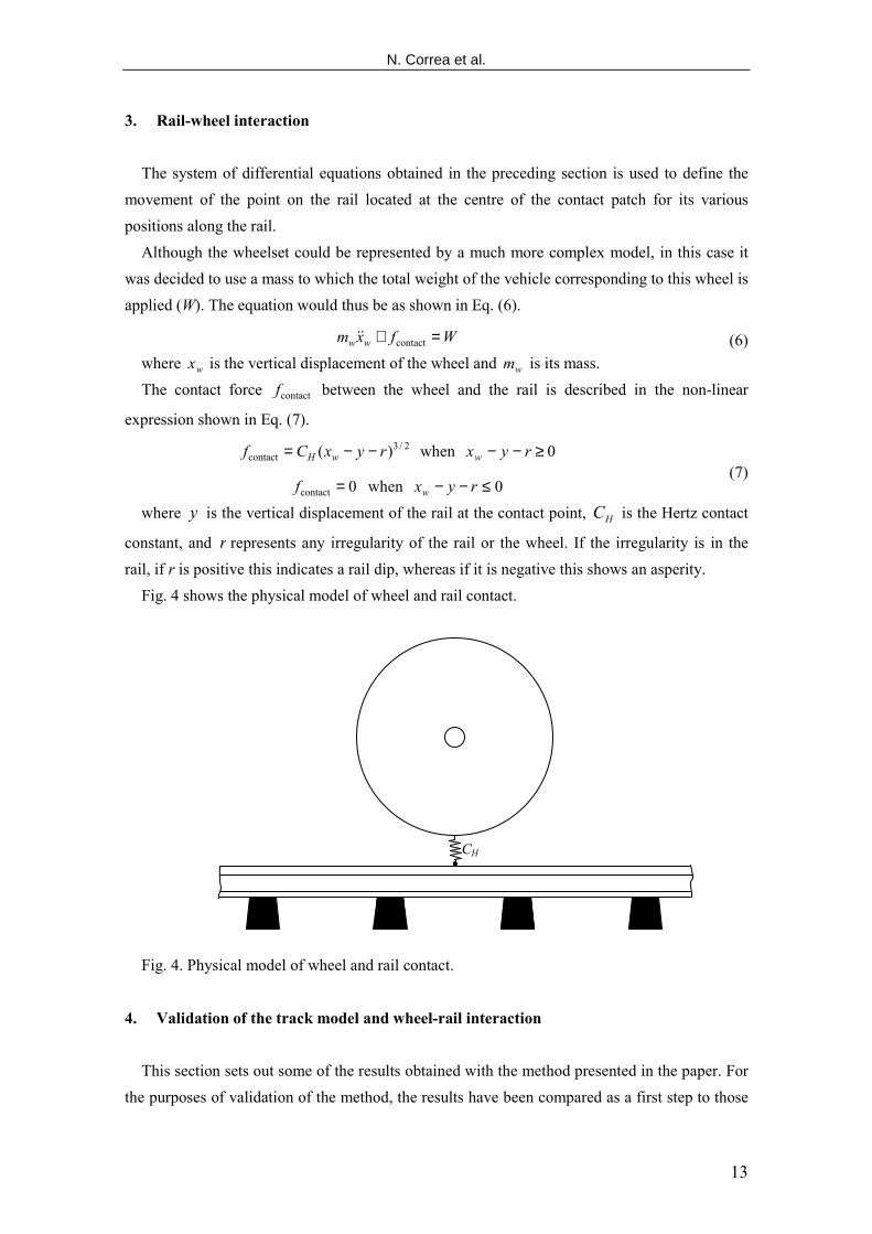
Although the wheelset could be represented by a much more complex model, in this case it

was decided to use a mass to which the total weight of the vehicle corresponding to this wheel is

applied (W). The equation would thus be as shown in Eq. (6).

Wfxm ww =+ contact&& (6)

where wx is the vertical displacement of the wheel and wm is its mass.

The contact force contactf between the wheel and the rail is described in the non-linear

expression shown in Eq. (7).

2/3contact )( ryxCf wH −−= when 0≥−− ryxw

0contact =f when 0≤−− ryxw (7)

where y is the vertical displacement of the rail at the contact point, HC is the Hertz contact

constant, and r represents any irregularity of the rail or the wheel. If the irregularity is in the

rail, if r is positive this indicates a rail dip, whereas if it is negative this shows an asperity.

Fig. 4 shows the physical model of wheel and rail contact.

Fig. 4. Physical model of wheel and rail contact.

4. Validation of the track model and wheel-rail interaction

This section sets out some of the results obtained with the method presented in the paper. For

the purposes of validation of the method, the results have been compared as a first step to those

CH


14

shown by Wu and Thompson [16,17]. It must be borne in mind that the initial receptances in

this work feature a number of differences with respect to Wu's and Thompson's receptances,

since they were obtained using different models, and thus the results of displacements after

integration may be slightly different. At a second step the new model has been validated against

Pieringer’s results [27].

Fig. 5 shows the comparison between the results obtained in paper [17] and those calculated

using the method described in this paper for displacements of the contact point on the wheel and

the rail at a speed of 36 m/s, when there is no irregularity on the rail surface (r = 0). The track

parameters are described in Table 1. The total weight of the vehicle corresponding to one wheel

and the unsprung mass are, respectively, W=100 kN and mw = 600 kg; and the elastic spring

constant is HC = 93.7 GNm-3/2

. The first instant represented on the figures corresponds to

movement over a sleeper, and shows movement over six spans of track. The Ss show the

position of the sleepers. Both Fig. 5a and 5b show that the main harmonic in the displacements

is that corresponding to the sleeper passage frequency, which in this case is 60 Hz. It may also

be observed that maximum dip at contact does not occur at exact midspan, but is displaced

slightly to the right.

Fig. 5. Displacements of wheel (--) and rail (−) when speed V = 36 m/s (a) obtained using the

method described herein, (b) obtained through [17].

(b)

(a)

N. Correa et al.

15

Fig. 6 shows the comparison between the displacements of wheel and rail when a wheel flat

exists calculated in accordance with this work and the displacements obtained through [16]. The

parameters used in this case are the same ones that those used for Fig. 5. This wheel flat was

defined using expression (8) [14].

−=l

zdr π2cos1

2 (8)

The depth of the defect (d) is 2 mm, and its total length (l) is 150 mm. Fig. 6 shows

superimposition of the displacements and representation of the defect. It may be observed that

the individual results are extremely similar. Likewise, Fig. 7 shows the contact force between

the wheel and the rail with this wheel flat. In both cases the force attains a maximum value

above 500 kN after the first loss of contact, and 200 kN after the second.

Fig. 6. Displacements of wheel (--) and rail (−) when speed V = 24 m/s and a wheel flat (-·-)

(a) obtained using the method described herein, (b) obtained through [16].

The results provided by the present model have also been compared to those published by

Pieringer and Kropp in [27]. Such a model is also linear in what regards to the track and

nonlinear in the contact, and has been applied to simulate wheel-rail interactions induced by

wheel flats. Pieringer and Kropp, on their turn, compare their own results to those

experimentally obtained by Johansson and Nielsen [28]. The results that follow have been

(b)

(a)


16

compared to both, the ones of [27] and [28]. The parameters of this track and case study are

shown in Table 2.

Fig. 7. Force of wheel and rail when speed V = 24 m/s and a wheel flat (a) obtained using the

method described herein, (b) obtained through [16].

Table 2: Track and vehicle parameters as described in [27]

Pad stiffness (kN/mm) 120

Pad damping (kNs/m) 16

Ballast stiffness (kN/mm) 140

Ballast damping (kNs/m) 165

Sleeper mass (kg) 250

Sleeper spacing (m) 0.65

Rail 60E1

Sprung mass W (t) 12

Unsprung mass (kg) 592.5

Wheel radius (m) 0.45

Fig. 8 shows the maximum contact forces produced by the wheel flat as defined in [27],

comparing the experimental results from [28], the numerical results obtained by Pieringer [27]

(b)

(a)

N. Correa et al.

17

and the ones obtained by the model presented in this paper. The wheel flat has been defined

according to expression (8), with 9.0=d mm and 1.0=l m.

Fig. 8. Comparison between the maximum forces measured experimentally by Johansson

[28] (measured values: • in blue, and curve fitted to their experimental results: continuous blue

line); Pieringer’s numerical results [27] (▪ in black); and results provided by the new model (in

red).

The experimental results by Johanson and Nielsen are shown as discrete values for several

vehicle speeds, together with the curve fit. Both Pieringer’s results and the ones obtained with

the present model are shown for each speed as a vertical segment or as a band, respectively,

taking account of the maximum and minimum values as a result of the position of the wheel flat

relative to the sleeper. It is shown that for speeds up to 100 km/h the results of the new model

are extremely similar to the curve by Johanson and Nielsen fitted to their experimental results.

And, despite the large conceptual differences between Pieringer’s model and the model

presented in this paper, both lead to results with reasonably similar trends.

Fig. 9 shows wheel and rail displacements when the wheelset, with the same wheel flat as

before, runs at 50 km/h along the same track. The sleeper is located al x=0. Fig. 9a shows the

results obtained by Pieringer in [27] and Fig. 9b shows the results provided by the method

developed. Fig. 10 compares wheel-rail contact forces, with the same criteria as above. As it can

be seen the results are reasonably similar for both forces and displacements, despite the great

differences between both models.

The differences between both results of the forces are at distance 0.08 m, where the wheel flat

starts, and a singular variation at distance 0.18 m, where the wheel flat ends. The beginning and


18

ending of the wheel flat is indicated with vertical dashed lines in Figs. 9 and 10. Both

differences are due to the dissimilar contact model used by each method.

Fig. 9. Wheel (--) and rail (-) displacements when the wheel flat runs at 50 km/h: (a) results

by Pieringer and (b) results of the new model.

(b)

(a)

(b)

(a)

N. Correa et al.

19

Fig. 10. Comparison between forces produced by a wheel flat at 50 km/h obtained by: (a)

results by Pieringer and (b) results of the new method.

5. Application of the method for modelling forces and displacements on movement over

a weld

Rail welds constitute one of the critical features of continuous welded rail (CWR). Depending

on the quality of the weld after grinding, large dynamic loads may arise as the wheelset moves

over the track, and even loss of contact and impacts in certain cases, when the irregularity

emerging from the weld is particularly large. Repeated movement of wheelsets over the welds

may cause cracks in the rail due to fatigue, and this can lead to breakage of the rail, a

particularly dangerous occurrence on the outside rail through a bend, since it could derail the

train.

Several rail infrastructure authorities are concerned with tendencies in weld surfaces, which

show dips after a number of years. As the wheelsets move over the rails, this effect is detected

as an impact similar to that caused by a wheelset moving over a flanged joint.

This section shows some of the results obtained for the track previously fitted using the

method set out herein, at different speeds, when the wheelset moves over the irregularity

emerging from the weld.

The method developed herein is particularly suited to this type of calculation, since it

reproduces the behaviour of the track extremely accurately, including the effect of the periodic

excitation when the vehicle moves over the sleepers, and the computational outlay of each

simulation is minimal.

Several welding geometry defects have been published as, for example, in [1, 29-31]. In the

present work the first welding geometry defect shown by Steenbergen in [31] has been chosen.

It is a welding experimentally measured by the author. A second welding geometry defect can

be found as well in [31], although it has not been used in this work because it exceeds the limits

described in the European Standard EN 14730-2 [3], which specifies the geometric

characteristics that rail welds must verify after grinding to be acceptable. Fig. 11 shows the

selected welding shape. In this dip the filtering effect due to the contact patch has already been

considered, and a continuous smoothing of five points (taking a 25 mm length) has been

performed.

Figs. 12 to 16 show the results of the wheel passing along the track described in Table 1, over

a welding irregularity as described in Fig. 11, being the dip located 10 cm before the sleeper.

The total weight of the vehicle corresponding to one wheel and the unsprung mass are,

respectively, W=100 kN and mw = 600 kg; and the elastic spring constant is HC = 93.7 GNm-3/2

.

Fig. 12 shows the displacements of the wheel and rail contact points, the contact force

generated when the wheel is moving at 40 km/h, and the rail surface irregularity at the weld. It


20

should be observed that the separation between the wheel and rail displacements is caused by

deformation on the contact due to the weight of the vehicle borne by the wheel. The

displacements' y-axis is inverted because displacements have been taken as positive when a dip

occurs, and as negative if this is not the case. Displacement of the rail surface has been

represented relative to the longitudinal geometry of the rail including the defect, in order to

appraise at what points in space loss of contact may occur (as it may happen for certain cases of

abnormal defects) and the impact when contact is retrieved. In the space before the weld defect,

the figure above to the right shows the influence of movement over the sleeper, which gives the

forces and displacements a periodic value rather than a constant value, with a spatial period

defined by the sleeper spacing (0.6 m). The figure above has been enlarged in the area

containing the weld for a better view of the forces and displacements in that area, and has been

represented on the figure below.

Fig. 11. Welding shape used [31].

At the beginning of the irregularity wheel and rail displacements are low, due to the fact that

the first part of the welding defect geometry is a slight and smooth elevation of the rail surface.

When the wheel commences the descent, as a result of the dipping on the rail surface in the

central area of the rail defect, the force falls very slightly. After this decrease, there is an

increase in the force during the defect’s upward ramp, leading to a contact force maximum 20%

above its average value. This is approximately twice the fluctuation of the force due to the

wheelset passage over sleeper and midspan, which, on its turn, is approximately 10% of the

static force supported by the wheel due to the vehicle weight.

N. Correa et al.

21

These figures also show that the excitation after the impact lasts over a very short space, and

that the effect of passage over the weld disappears almost as the wheel reaches the end of the

irregularity.

In the case of Fig. 13, where the results of the simulation at a running speed of 60 km/h are

shown, forces reach 134 kN. Given the higher speed, the duration of the excitation after passing

over the welding defect is also longer, although it still remains very low.

Fig. 12. (a) Displacements of wheel (--) and rail (−) at contact. (b) Irregularity (--) and contact

forces (−) for a speed of 40 km/h.

(a)

(b)


22



Fig. 14 shows displacements and forces calculated for a running speed of 80 km/h. In this

case the contact force reaches a maximum value of circa 144 kN, i.e. 44% above the static force

due to the weight of the vehicle on the wheel.

(a)

(b)

N. Correa et al.

23



Fig. 15 shows the contact forces for all three speeds. For these speeds, this track, and this

location of the welding dip, it can be observed that the maximum forces in the contact increase

with speed. It is also shown that the effect of passage over the weld is maintained over a greater

distance when the speed is increased.

Parametric excitation has a significant importance in wheel-rail interactions, as already

mentioned. The sleeper positioning considerably affects the dynamic wheel-rail interaction, and

the model developed is able to take this into account. Therefore this capability has been used to

quantify the influence on the wheel-rail forces of the defect position relative to the sleeper, in a

similar way to what was mentioned previously in relation to the wheel flat positioning relative

to the sleeper.

Fig. 16 shows the comparison between calculated forces when the welding is located at

different positions. These results have been obtained for a wheelset running at a speed of 80

km/h on a track whose receptances are the ones shown in Fig. 1. In this figure line 0L

corresponds to the welding located at the rail section above a sleeper, 0.25L is the response

when the welding is located at a quarter span distance from that sleeper, 0.5L when the defect is

just at midspan, and 0.75L is the response if the welding defect is at three quarter span from the

previous sleeper.

(a)

(b)


24

Fig. 15. Comparison of contact forces for: speed 40 km/h (-·-), speed 60 km/h (−), and speed

80 km/h (--).

Fig. 16. Contact forces from welding defects at different positions within a span.

It can be seen that the largest forces appear when the welding defect is at a rail section

located above the sleeper, reaching for this type of track and vehicle a maximum force of 144

N. Correa et al.

25

kN, whereas the minimum forces appear when the welding defect is at midspan, reaching in this

case 134 kN.

These forces are higher than usual. After a comparison of the forces obtained for different

track parameters, it is concluded that in the present case the track is considerably stiff, leading

therefore to such high forces. Slight reductions in track stiffness provoke the maximum forces to

decrease up to 10 kN. For the case of the track described in [31] and with the same dip as

before, even though the present model and the model described in that paper are based on

completely different assumptions, the maximum forces provided by the present model for a

speed of 140 km/h are lower than the ones published in that paper: 125,7 kN of total maximum

force with the present method, against approximately 129,5 kN of total maximum force (17 kN

of dynamic force) obtained in [31].

6. Conclusions

A method has been developed to improve and facilitate the passage of track models in the

frequency domain to models in the spatial domain. This can be a very interesting procedure

when an extremely precise model in the frequency domain is available which, in comparison to

the usual spatial-domain models, can take account to a high degree of accuracy of the track's

dynamic behaviour, including deformation of the rail section and the propagation of elongation,

bending and buckling waves, and the intention is to make use of the advantages of this model

with respect to more simplified models in the spatial domain. Moreover, the model produced by

this method is very simple, with very few degrees of freedom, thus compensating the time

required for passage to the spatial domain with a substantial reduction of simulation time.

The method developed is based on the receptances obtained using the model in the frequency

domain on track sections in as close proximity as is desired, and this secures a model in the

spatial domain that adjusts to these receptances. To this end the process is based on application

of the rational fraction polynomials method, with a weight vector at each frequency of the fitting

optimised using genetic algorithms, in order to obtain the best possible fit of track receptances.

The result of this fitting is a transfer function the frequency response of which represents a good

fit for the track receptance, and which can be transformed into a system of ordinary differential

equations by applying the inverse Laplace transform. This fitting is repeated for different

sections of the track span, and the result obtained is a system of equations in the spatial domain

which varies along the track span. The method also guarantees the stability of the resultant

system in the spatial domain and the fitting coefficients set, which facilitate integration of the

system of equations.

The method has been validated with the results obtained by Wu and Thompson [16,17] and

by Pieringer [27]. The model is applicable to most wheel-rail dynamic interaction problems, and


26

it has been applied to the study of the displacements and forces that emerge when the wheelset

moves over a weld. It has been possible to compare the increase in the contact forces produced

by the welding defect with the increase in such forces as a result of the parametric excitation

due to the discrete support. Welding defects complying with international standards have been

studied and contact forces and displacements have been calculated at different speeds. The

model has been used to quantify the influence of the welding being over a sleeper, on the centre

of the span or at intermediate locations.

Acknowledgements

The authors thank the Spanish Research Ministry MICINN for their funding through contract

TRA2010-18386 including the FEDER funds of the European Union, as well as the Basque

Government for its financial assistance through IT-453-10 and for Research Grant BFI08.172.

They also thank the Basque Railway Infrastructure Manager ETS/RFV and Metro Bilbao for

their assistance and valuable suggestions.

References

[1] M. J. M. M. Steenbergen, C. Esveld. Rail weld geometry and assessment concepts,

Proceedings of the IMechE, Part F: Journal of Rail and Rapid Transit, 2006, 220 (F3), 257-271.

[2] M. J. M. M. Steenbergen, C Esveld. Relation between the geometry of rail welds and the

dynamic wheel - rail response: numerical simulations for measured welds, Proceedings of the

IMechE, Part F, Journal of Rail and Rapid Transit, 2006, 220 (F4), 409-424.

[3] EN 14730-2:2006. Railway applications. Track. Aluminothermic welding of rails.

Qualifications of aluminothermic welders, approval of contractors and acceptance of welds.

[4] A. V. Vostroukhov, A. V. Metrikine. Periodically supported beam on a visco-elastic layer as

a model for dynamic analysis of a high-speed railway track, International Journal of Solids and

Structures. 40 (2003) 5723-5752.

[5] M. F. M. Hussein, H. E. M. Hunt. Modelling of floating-slab tracks with continuous slabs

under oscillating moving loads, Journal of Sound and Vibration. 297 (2006) 37-54.

[6] I. Gómez, E. G. Vadillo. An analytical approach to study a special case of booted sleeper

track rail corrugation, Wear. 251 (2001) 916-924.

N. Correa et al.

27

[7] I. Gómez, E. G. Vadillo. A linear model to explain short pitch corrugation on rails, Wear.

255 (2003) 1127-1142.

[8] J. Gómez, E. G. Vadillo, J Santamaría. A comprehensive track model for the improvement

of corrugation models, Journal of Sound and Vibration. 293 (2006) 522-534.

[9] O. Oyarzabal, J. Gómez, J. Santamaría, E. G. Vadillo. Dynamic optimization of track

components to minimize rail corrugation, Journal of Sound and Vibration. 319 (2009) 904-917.

[10] T. Mazilu. Green's functions for analysis of dynamic response of wheel/rail to vertical

excitation, Journal of Sound and Vibration. 306 (2007) 31-58.

[11] T. Mazilu, M. Dumitriu, C. Tudorache, M. Sebeşan. Using the Green’s functions method to

study wheelset/ballasted track vertical interaction, Mathematical Computer Modelling. 54

(2011) 261-279.

[12] T. X. Wu, D. J. Thompson. Theoretical investigation of wheel/rail non-linear interaction

due to roughness excitation, Vehicle System Dynamics. 34 (2000) 261-282.

[13] T. X. Wu, D. J. Thompson. A hybrid model for the noise generation due to railway wheel

flats, Journal of Sound and Vibration. 251 (2002) 115-139.

[14] T. X. Wu, D. J. Thompson. On the impact noise generation due to a wheel passing over rail

joints, Journal of Sound and Vibration. 267 (2003) 485-496.

[15] T. X. Wu, D. J. Thompson. Wheel/rail non-linear interactions with coupling between

vertical and lateral directions, Vehicle System Dynamics. 41 (2004) 27-49.

[16] T. X. Wu, D. J. Thompson. On the parametric excitation of the wheel/track system, Journal

of Sound and Vibration. 278 (2004) 725-747.

[17] T. X. Wu, D. J. Thompson. On the rolling noise generation due to wheel/track parametric

excitation, Journal of Sound and Vibration. 293 (2006) 566-574.

[18] T. X. Wu. Parametric excitation of wheel/track system and its effects on rail corrugation,

Wear. 265 (2008) 1176-1182.

[19] G. Bonin, G. Cantisani, M. Carbonari, G. Loprencipe, A. Pancotto, Railway traffic

vibrations: generation and propagation - Theoretical aspects, 4th International SIIV Congress -

Palermo (Italy). (2007).


28

[20] G. Bonin, G. Cantisani, M. Carbonari, G. Loprencipe, A. Pancotto, Railway traffic

vibrations: generation and propagation - Use of computational models, 4th International SIIV

Congress - Palermo (Italy). (2007).

[21] M.H. Richardson, D. L. Formenti, Parameter estimation from frequency response

measurements using rational fraction polynomials. (1982).

[22] F. H. Raven, Automatic control Engineering, 4th ed. ed., McGraw-Hill, New York, 1987.

[23] R. Taghipour, T. Perez, T. Moan. Hybrid frequency–time domain models for dynamic

response analysis of marine structures, Ocean Engineering. 35 (2008) 685-705.

[24] The MathWorks Inc., Optimization Toolbox™ User’s Guide, 2010.

[25] The MathWorks Inc., Global Optimization Toolbox User’s Guide, 2010.

[26] The MathWorks Inc., Signal Processing Toolbox™ User’s Guide, 2010.

[27] A. Pieringer, W. Kropp, A fast-time-domain model for wheel/rail interaction demonstrated

for the case of impact forces caused by wheel flats. Proceedings of Acoustics '08, Paris, France,

June 29-July 4, 2008.

[28] A. Johansson, J. C. O. Nielsen. Out-of-round railway wheels—wheel-rail contact forces

and track response derived from field tests and numerical simulations, Proceedings of the

Institution of Mechanical Engineers, Part F: Journal of Rail and Rapid Transit. 217 (2003) 135-

146.

[29] W. Li, G. Xiao, Z. Wen, X Xiao, X. Jin. Plastic deformation of curved rail at rail weld

caused by train–track dynamic interaction, Wear. 271 (2011) 311-318.

[30] Z. Wen, G. Xiao, X. Xiao, X. Jin, M. Zhu. Dynamic vehicle–track interaction and plastic

deformation of rail at rail welds, Engineering Failure Analysis. 16 (2009) 1221-1237.

[31] M. J. M. M. Steenbergen. Quantification of dynamic wheel–rail contact forces at short rail

irregularities and application to measured rail welds, Journal of Sound and Vibration. 312

(2008) 606-629.

A rational fraction polynomials model to study vertical ...

Documents