The Annals of Applied Probability 2018, Vol. 28, No. 2, 1190–1248 https://doi.org/10.1214/17-AAP1328 © Institute of Mathematical Statistics, 2018 A RANDOM MATRIX APPROACH TO NEURAL NETWORKS BY COSME LOUART,ZHENYU LIAO AND ROMAIN COUILLET 1 CentraleSupélec, University of Paris–Saclay This article studies the Gram random matrix model G = 1 T T , = σ(WX), classically found in the analysis of random feature maps and ran- dom neural networks, where X =[x 1 ,...,x T ]∈ R p×T is a (data) ma- trix of bounded norm, W ∈ R n×p is a matrix of independent zero-mean unit variance entries and σ : R → R is a Lipschitz continuous (activation) function—σ(WX) being understood entry-wise. By means of a key concen- tration of measure lemma arising from nonasymptotic random matrix argu- ments, we prove that, as n,p,T grow large at the same rate, the resolvent Q = (G + γI T ) −1 , for γ> 0, has a similar behavior as that met in sam- ple covariance matrix models, involving notably the moment = T n E[G], which provides in passing a deterministic equivalent for the empirical spec- tral measure of G. Application-wise, this result enables the estimation of the asymptotic performance of single-layer random neural networks. This in turn provides practical insights into the underlying mechanisms into play in ran- dom neural networks, entailing several unexpected consequences, as well as a fast practical means to tune the network hyperparameters. CONTENTS 1. Introduction ............................................ 1191 2. System model ........................................... 1193 3. Main results ............................................ 1196 3.1. Main technical results and training performance ..................... 1196 3.2. Testing performance .................................... 1199 3.3. Evaluation of AB ..................................... 1200 4. Practical outcomes ........................................ 1202 4.1. Simulation results ...................................... 1202 4.2. The underlying kernel .................................... 1203 4.3. Limiting cases ........................................ 1207 5. Proof of the main results ..................................... 1209 5.1. Concentration results on ................................. 1209 5.2. Asymptotic equivalents ................................... 1219 5.2.1. First equivalent for E[Q] .............................. 1219 5.2.2. Second equivalent for E[Q] ............................. 1223 5.2.3. Asymptotic equivalent for E[QAQ], where A is either or symmetric of bounded norm .................................... 1225 5.3. Derivation of ab ...................................... 1230 Received February 2017; revised June 2017. 1 Supported by the ANR Project RMT4GRAPH (ANR-14-CE28-0006). MSC2010 subject classifications. Primary 60B20; secondary 62M45. Key words and phrases. Random matrix theory, random feature maps, neural networks. 1190

Welcome message from author
This document is posted to help you gain knowledge. Please leave a comment to let me know what you think about it! Share it to your friends and learn new things together.
Transcript
The Annals of Applied Probability2018, Vol. 28, No. 2, 1190–1248https://doi.org/10.1214/17-AAP1328© Institute of Mathematical Statistics, 2018
A RANDOM MATRIX APPROACH TO NEURAL NETWORKS
BY COSME LOUART, ZHENYU LIAO AND ROMAIN COUILLET1
CentraleSupélec, University of Paris–Saclay
This article studies the Gram random matrix model G = 1T
�T�, � =σ(WX), classically found in the analysis of random feature maps and ran-dom neural networks, where X = [x1, . . . , xT ] ∈ R
p×T is a (data) ma-trix of bounded norm, W ∈ R
n×p is a matrix of independent zero-meanunit variance entries and σ : R → R is a Lipschitz continuous (activation)function—σ(WX) being understood entry-wise. By means of a key concen-tration of measure lemma arising from nonasymptotic random matrix argu-ments, we prove that, as n,p,T grow large at the same rate, the resolventQ = (G + γ IT )−1, for γ > 0, has a similar behavior as that met in sam-ple covariance matrix models, involving notably the moment � = T
n E[G],which provides in passing a deterministic equivalent for the empirical spec-tral measure of G. Application-wise, this result enables the estimation of theasymptotic performance of single-layer random neural networks. This in turnprovides practical insights into the underlying mechanisms into play in ran-dom neural networks, entailing several unexpected consequences, as well asa fast practical means to tune the network hyperparameters.
CONTENTS
1. Introduction . . . . . . . . . . . . . . . . . . . . . . . . . . . . . . . . . . . . . . . . . . . . 11912. System model . . . . . . . . . . . . . . . . . . . . . . . . . . . . . . . . . . . . . . . . . . . 11933. Main results . . . . . . . . . . . . . . . . . . . . . . . . . . . . . . . . . . . . . . . . . . . . 1196
3.1. Main technical results and training performance . . . . . . . . . . . . . . . . . . . . . 11963.2. Testing performance . . . . . . . . . . . . . . . . . . . . . . . . . . . . . . . . . . . . 11993.3. Evaluation of �AB . . . . . . . . . . . . . . . . . . . . . . . . . . . . . . . . . . . . . 1200
4. Practical outcomes . . . . . . . . . . . . . . . . . . . . . . . . . . . . . . . . . . . . . . . . 12024.1. Simulation results . . . . . . . . . . . . . . . . . . . . . . . . . . . . . . . . . . . . . . 12024.2. The underlying kernel . . . . . . . . . . . . . . . . . . . . . . . . . . . . . . . . . . . . 12034.3. Limiting cases . . . . . . . . . . . . . . . . . . . . . . . . . . . . . . . . . . . . . . . . 1207
5. Proof of the main results . . . . . . . . . . . . . . . . . . . . . . . . . . . . . . . . . . . . . 12095.1. Concentration results on � . . . . . . . . . . . . . . . . . . . . . . . . . . . . . . . . . 12095.2. Asymptotic equivalents . . . . . . . . . . . . . . . . . . . . . . . . . . . . . . . . . . . 1219
5.2.1. First equivalent for E[Q] . . . . . . . . . . . . . . . . . . . . . . . . . . . . . . 12195.2.2. Second equivalent for E[Q] . . . . . . . . . . . . . . . . . . . . . . . . . . . . . 12235.2.3. Asymptotic equivalent for E[QAQ], where A is either � or symmetric of
bounded norm . . . . . . . . . . . . . . . . . . . . . . . . . . . . . . . . . . . . 12255.3. Derivation of �ab . . . . . . . . . . . . . . . . . . . . . . . . . . . . . . . . . . . . . . 1230
Received February 2017; revised June 2017.1Supported by the ANR Project RMT4GRAPH (ANR-14-CE28-0006).MSC2010 subject classifications. Primary 60B20; secondary 62M45.Key words and phrases. Random matrix theory, random feature maps, neural networks.
1190
A RANDOM MATRIX APPROACH TO NEURAL NETWORKS 1191
5.3.1. Gaussian w . . . . . . . . . . . . . . . . . . . . . . . . . . . . . . . . . . . . . . 12305.4. Polynomial σ(·) and generic w . . . . . . . . . . . . . . . . . . . . . . . . . . . . . . . 12335.5. Heuristic derivation of Conjecture 1 . . . . . . . . . . . . . . . . . . . . . . . . . . . . 1233
6. Concluding remarks . . . . . . . . . . . . . . . . . . . . . . . . . . . . . . . . . . . . . . . 1243Appendix: Intermediary lemmas . . . . . . . . . . . . . . . . . . . . . . . . . . . . . . . . . . 1245References . . . . . . . . . . . . . . . . . . . . . . . . . . . . . . . . . . . . . . . . . . . . . . 1246
1. Introduction. Artificial neural networks, developed in the late fifties[Rosenblatt (1958)] in an attempt to develop machines capable of brain-like behav-iors, know today an unprecedented research interest, notably in its applications tocomputer vision and machine learning at large [Krizhevsky, Sutskever and Hinton(2012), Schmidhuber (2015)] where superhuman performances on specific tasksare now commonly achieved. Recent progress in neural network performanceshowever find their source in the processing power of modern computers as well asin the availability of large datasets rather than in the development of new math-ematics. In fact, for lack of appropriate tools to understand the theoretical be-havior of the nonlinear activations and deterministic data dependence underlyingthese networks, the discrepancy between mathematical and practical (heuristic)studies of neural networks has kept widening. A first salient problem in harness-ing neural networks lies in their being completely designed upon a deterministictraining dataset X = [x1, . . . , xT ] ∈ R
p×T , so that their resulting performancesintricately depend first and foremost on X. Recent works have nonetheless es-tablished that, when smartly designed, mere randomly connected neural networkscan achieve performances close to those reached by entirely data-driven networkdesigns [Rahimi and Recht (2007), Saxe et al. (2011)]. As a matter of fact, to han-dle gigantic databases, the computationally expensive learning phase (the so-calledbackpropagation of the error method) typical of deep neural network structures be-comes impractical, while it was recently shown that smartly designed single-layerrandom networks (as studied presently) can already reach superhuman capabilities[Cambria et al. (2015)] and beat expert knowledge in specific fields [Jaeger andHaas (2004)]. These various findings have opened the road to the study of neu-ral networks by means of statistical and probabilistic tools [Choromanska et al.(2015), Giryes, Sapiro and Bronstein (2016)]. The second problem relates to thenonlinear activation functions present at each neuron, which have long been known(as opposed to linear activations) to help design universal approximators for anyinput–output target map [Hornik, Stinchcombe and White (1989)].
In this work, we propose an original random matrix-based approach to under-stand the end-to-end regression performance of single-layer random artificial neu-ral networks, sometimes referred to as extreme learning machines [Huang, Zhuand Siew (2006), Huang et al. (2012)], when the number T and size p of the in-put dataset are large and scale proportionally with the number n of neurons inthe network. These networks can also be seen, from a more immediate statis-tical viewpoint, as a mere linear ridge-regressor relating a random feature map

1192 C. LOUART, Z. LIAO AND R. COUILLET
σ(WX) ∈ Rn×T of explanatory variables X = [x1, . . . , xT ] ∈ R
p×T and targetvariables y = [y1, . . . , yT ] ∈ R
d×T , for W ∈ Rn×p a randomly designed matrix
and σ(·) a nonlinear R → R function (applied component-wise). Our approachhas several interesting features both for theoretical and practical considerations.It is first one of the few known attempts to move the random matrix realm awayfrom matrices with independent or linearly dependent entries. Notable exceptionsare the line of works surrounding kernel random matrices [Couillet and Benaych-Georges (2016), El Karoui (2010)] as well as large dimensional robust statisticsmodels [Couillet, Pascal and Silverstein (2015), El Karoui (2013), Zhang, Chengand Singer (2014)]. Here, to alleviate the nonlinear difficulty, we exploit concentra-tion of measure arguments [Ledoux (2005)] for nonasymptotic random matrices,thereby pushing further the original ideas of El Karoui (2009), Vershynin (2012)established for simpler random matrix models. While we believe that more power-ful, albeit more computational intensive, tools [such as an appropriate adaptationof the Gaussian tools advocated in Pastur and Serbina (2011)] cannot be avoided tohandle advanced considerations in neural networks, we demonstrate here that theconcentration of measure phenomenon allows one to fully characterize the mainquantities at the heart of the single-layer regression problem at hand.
In terms of practical applications, our findings shed light on the already in-completely understood extreme learning machines which have proved extremelyefficient in handling machine learning problems involving large to huge datasets[Cambria et al. (2015), Huang et al. (2012)] at a computationally affordable cost.But our objective is also to pave to path to the understanding of more involved neu-ral network structures, featuring notably multiple layers and some steps of learningby means of backpropagation of the error.
Our main contribution is twofold. From a theoretical perspective, we first ob-tain a key lemma, Lemma 1, on the concentration of quadratic forms of thetype σ(wTX)Aσ(XTw) where w = ϕ(w), w ∼ N (0, Ip), with ϕ : R → R andσ : R → R Lipschitz functions, and X ∈ R
p×T , A ∈ Rn×n are deterministic ma-
trices. This nonasymptotic result (valid for all n,p,T ) is then exploited under asimultaneous growth regime for n,p,T and boundedness conditions on ‖X‖ and‖A‖ to obtain, in Theorem 1, a deterministic approximation Q of the resolventE[Q], where Q = ( 1
T�T� + γ IT )−1, γ > 0, � = σ(WX), for some W = ϕ(W ),
W ∈ Rn×p having independent N (0,1) entries. As the resolvent of a matrix (or
operator) is an important proxy for the characterization of its spectrum [see, e.g.,Akhiezer and Glazman (1993), Pastur and Serbina (2011)], this result therefore al-lows for the characterization of the asymptotic spectral properties of 1
T�T�, such
as its limiting spectral measure in Theorem 2.Application-wise, the theoretical findings are an important preliminary step for
the understanding and improvement of various statistical methods based on ran-dom features in the large dimensional regime. Specifically, here, we consider thequestion of linear ridge-regression from random feature maps, which coincides
A RANDOM MATRIX APPROACH TO NEURAL NETWORKS 1193
with the aforementioned single hidden-layer random neural network known as ex-treme learning machine. We show that, under mild conditions, both the trainingEtrain and testing Etest mean-square errors, respectively, corresponding to the re-gression errors on known input–output pairs (x1, y1), . . . , (xT , yT ) (with xi ∈ R
p ,yi ∈ R
d ) and unknown pairings (x1, y1), . . . , (xT, y
T), almost surely converge to
deterministic limiting values as n,p,T grow large at the same rate (while d iskept constant) for every fixed ridge-regression parameter γ > 0. Simulations onreal image datasets are provided that corroborate our results.
These findings provide new insights into the roles played by the activation func-tion σ(·) and the random distribution of the entries of W in random feature maps aswell as by the ridge-regression parameter γ in the neural network performance. Wenotably exhibit and prove some peculiar behaviors, such as the impossibility forthe network to carry out elementary Gaussian mixture classification tasks, wheneither the activation function or the random weights distribution are ill chosen.
Besides, for the practitioner, the theoretical formulas retrieved in this work al-low for a fast offline tuning of the aforementioned hyperparameters of the neuralnetwork, notably when T is not too large compared to p. The graphical resultsprovided in the course of the article were particularly obtained within a 100- to500-fold gain in computation time between theory and simulations.
The remainder of the article is structured as follows: in Section 2, we introducethe mathematical model of the system under investigation. Our main results arethen described and discussed in Section 3, the proofs of which are deferred toSection 5. Section 4 discusses our main findings. The article closes on concludingremarks on envisioned extensions of the present work in Section 6. The Appendixprovides some intermediary lemmas of constant use throughout the proof section.
Reproducibility: Python 3 codes used to produce the results of Section 4 areavailable at https://github.com/Zhenyu-LIAO/RMT4ELM.
Notation: The norm ‖ · ‖ is understood as the Euclidean norm for vectors andthe operator norm for matrices, while the norm ‖ · ‖F is the Frobenius norm formatrices. All vectors in the article are understood as column vectors.
2. System model. We consider a ridge-regression task on random featuremaps defined as follows. Each input data x ∈ R
p is multiplied by a matrixW ∈ R
n×p; a nonlinear function σ : R → R is then applied entry-wise to thevector Wx, thereby providing a set of n random features σ(Wx) ∈ R
n for eachdatum x ∈ R
p . The output z ∈ Rd of the linear regression is the inner product
z = βTσ(Wx) for some matrix β ∈ Rn×d to be designed.
From a neural network viewpoint, the n neurons of the network are the virtualunits operating the mapping Wi·x �→ σ(Wi·x) (Wi· being the ith row of W ), for1 ≤ i ≤ n. The neural network then operates in two phases: a training phase wherethe regression matrix β is learned based on a known input–output dataset pair(X,Y ) and a testing phase where, for β now fixed, the network operates on a newinput dataset X with corresponding unknown output Y .
1194 C. LOUART, Z. LIAO AND R. COUILLET
During the training phase, based on a set of known input X = [x1, . . . , xT ] ∈R
p×T and output Y = [y1, . . . , yT ] ∈ Rd×T datasets, the matrix β is chosen so
as to minimize the mean square error 1T
∑Ti=1 ‖zi − yi‖2 + γ ‖β‖2
F , where zi =βTσ(Wxi) and γ > 0 is some regularization factor. Solving for β , this leads to theexplicit ridge-regressor
β = 1
T�
(1
T�T� + γ IT
)−1Y T,
where we defined � ≡ σ(WX). This follows from differentiating the mean squareerror along β to obtain 0 = γβ + 1
T
∑Ti=1 σ(Wxi)(β
Tσ(Wxi) − yi)T, so that
( 1T��T + γ In)β = 1
T�Y T which, along with ( 1
T��T + γ In)
−1� = �( 1T
�T� +γ IT )−1, gives the result.
In the remainder, we will also denote
Q ≡(
1
T�T� + γ IT
)−1
the resolvent of 1T�T�. The matrix Q naturally appears as a key quantity in the
performance analysis of the neural network. Notably, the mean-square error Etrainon the training dataset X is given by
Etrain = 1
T
∥∥Y T − �Tβ∥∥2F = γ 2
TtrY TYQ2.(1)
Under the growth rate assumptions on n,p,T taken below, it shall appear that therandom variable Etrain concentrates around its mean, letting then appear E[Q2] asa central object in the asymptotic evaluation of Etrain.
The testing phase of the neural network is more interesting in practice as it
unveils the actual performance of neural networks. For a test dataset X ∈ Rp×T of
length T , with unknown output Y ∈ Rd×T , the test mean-square error is defined
by
Etest = 1
T
∥∥Y T − �Tβ∥∥2F ,
where � = σ(WX) and β is the same as used in (1) [and thus only dependson (X,Y ) and γ ]. One of the key questions in the analysis of such an elemen-tary neural network lies in the determination of γ which minimizes Etest (and isthus said to have good generalization performance). Notably, small γ values areknown to reduce Etrain but to induce the popular overfitting issue which gener-ally increases Etest, while large γ values engender both large values for Etrain andEtest.
From a mathematical standpoint though, the study of Etest brings forward sometechnical difficulties that do not allow for as a simple treatment through the presentconcentration of measure methodology as the study of Etrain. Nonetheless, the

A RANDOM MATRIX APPROACH TO NEURAL NETWORKS 1195
analysis of Etrain allows at least for heuristic approaches to become available,which we shall exploit to propose an asymptotic deterministic approximation forEtest.
From a technical standpoint, we shall make the following set of assumptions onthe mapping x �→ σ(Wx).
ASSUMPTION 1 (Sub-Gaussian W ). The matrix W is defined by
W = ϕ(W )
(understood entry-wise), where W has independent and identically distributedN (0,1) entries and ϕ(·) is λϕ-Lipschitz.
For a = ϕ(b) ∈ R, ≥ 1, with b ∼ N (0, I), we shall subsequently denote
a ∼Nϕ(0, I).Under the notation of Assumption 1, we have in particular Wij ∼ N (0,1) if
ϕ(t) = t and Wij ∼ U(−1,1) (the uniform distribution on [−1,1]) if ϕ(t) = −1 +2 1√
2π
∫∞t e−x2
dx (ϕ is here a√
2/π -Lipschitz map).We further need the following regularity condition on the function σ .
ASSUMPTION 2 (Function σ ). The function σ is Lipschitz continuous withparameter λσ .
This assumption holds for many of the activation functions traditionally con-sidered in neural networks, such as sigmoid functions, the rectified linear unitσ(t) = max(t,0) or the absolute value operator.
When considering the interesting case of simultaneously large data and ran-dom features (or neurons), we shall then make the following growth rate assump-tions.
ASSUMPTION 3 (Growth rate). As n → ∞,
0 < lim infn
min{p/n,T /n} ≤ lim supn
max{p/n,T /n} < ∞
while γ,λσ , λϕ > 0 and d are kept constant. In addition,
lim supn
‖X‖ < ∞,
lim supn
maxij
|Yij | < ∞.
1196 C. LOUART, Z. LIAO AND R. COUILLET
3. Main results.
3.1. Main technical results and training performance. As a standard prelimi-nary step in the asymptotic random matrix analysis of the expectation E[Q] of theresolvent Q = ( 1
T�T� + γ IT )−1, a convergence of quadratic forms based on the
row vectors of � is necessary [see, e.g., Marcenko and Pastur (1967), Silversteinand Bai (1995)]. Such results are usually obtained by exploiting the independence(or linear dependence) in the vector entries. This not being the case here, as theentries of the vector σ(XTw) are in general not independent, we resort to a con-centration of measure approach, as advocated in El Karoui (2009). The followinglemma, stated here in a nonasymptotic random matrix regime (i.e., without neces-sarily resorting to Assumption 3), and thus of independent interest, provides thisconcentration result. For this lemma, we need first to define the following key ma-trix:
� = E[σ(wTX
)Tσ(wTX
)](2)
of size T × T , where w ∼ Nϕ(0, Ip).
LEMMA 1 (Concentration of quadratic forms). Let Assumptions 1–2 hold. Letalso A ∈ R
T ×T such that ‖A‖ ≤ 1 and, for X ∈ Rp×T and w ∼ Nϕ(0, Ip), define
the random vector σ ≡ σ(wTX)T ∈ RT . Then
P
(∣∣∣∣ 1T σ TAσ − 1
Ttr�A
∣∣∣∣> t
)≤ Ce
− cT
‖X‖2λ2ϕλ2
σmin( t2
t20,t)
for t0 ≡ |σ(0)| + λϕλσ‖X‖√
pT
and C,c > 0 independent of all other parameters.In particular, under the additional Assumption 3,
P
(∣∣∣∣ 1T σ TAσ − 1
Ttr�A
∣∣∣∣> t
)≤ Ce−cnmin(t,t2)
for some C,c > 0.
Note that this lemma partially extends concentration of measure results involv-ing quadratic forms [see, e.g., Rudelson, Vershynin et al. (2013), Theorem 1.1], tononlinear vectors.
With this result in place, the standard resolvent approaches of random matrixtheory apply, providing our main theoretical finding as follows.
THEOREM 1 (Asymptotic equivalent for E[Q]). Let Assumptions 1–3 holdand define Q as
Q ≡(
n
T
�
1 + δ+ γ IT
)−1,
A RANDOM MATRIX APPROACH TO NEURAL NETWORKS 1197
where δ is implicitly defined as the unique positive solution to δ = 1T
tr�Q. Then,for all ε > 0, there exists c > 0 such that∥∥E[Q] − Q
∥∥≤ cn− 12 +ε.
As a corollary of Theorem 1 along with a concentration argument on 1T
trQ, wehave the following result on the spectral measure of 1
T�T�, which may be seen as
a nonlinear extension of Silverstein and Bai (1995) for which σ(t) = t .
THEOREM 2 (Limiting spectral measure of 1T�T�). Let Assumptions 1–3
hold and, for λ1, . . . , λT the eigenvalues of 1T�T�, define μn = 1
T
∑Ti=1 δλi
. Then,for every bounded continuous function f , with probability one∫
f dμn −∫
f dμn → 0,
where μn is the measure defined through its Stieltjes’ transform mμn(z) ≡ ∫ (t −z)−1 dμn(t) given, for z ∈ {w ∈C,�[w] > 0}, by
mμn(z) = 1
Ttr(
n
T
�
1 + δz
− zIT
)−1
with δz the unique solution in {w ∈ C,�[w] > 0} of
δz = 1
Ttr�(
n
T
�
1 + δz
− zIT
)−1.
Note that μn has a well-known form, already met in early random matrixworks [e.g., Silverstein and Bai (1995)] on sample covariance matrix models. No-tably, μn is also the deterministic equivalent of the empirical spectral measure of1TP TWTWP for any deterministic matrix P ∈ R
p×T such that P TP = �. As such,to some extent, the results above provide a consistent asymptotic linearizationof 1
T�T�. From standard spiked model arguments [see, e.g., Benaych-Georges
and Nadakuditi (2012)], the result ‖E[Q] − Q‖ → 0 further suggests that also theeigenvectors associated to isolated eigenvalues of 1
T�T� (if any) behave similarly
to those of 1TP TWTWP , a remark that has fundamental importance in the neural
network performance understanding.However, as shall be shown in Section 3.3, and contrary to empirical covariance
matrix models of the type P TWTWP , � explicitly depends on the distribution ofWij (i.e., beyond its first two moments). Thus, the aforementioned linearizationof 1
T�T�, and subsequently the deterministic equivalent for μn, are not universal
with respect to the distribution of zero-mean unit variance Wij . This is in strikingcontrast to the many linear random matrix models studied to date which oftenexhibit such universal behaviors. This property too will have deep consequences inthe performance of neural networks as shall be shown through Figure 3 in Section 4

1198 C. LOUART, Z. LIAO AND R. COUILLET
for an example where inappropriate choices for the law of W lead to networkfailure to fulfill the regression task.
For convenience in the following, letting δ and � be defined as in Theorem 1,we shall denote
= n
T
�
1 + δ.(3)
Theorem 1 provides the central step in the evaluation of Etrain, for which notonly E[Q] but also E[Q2] needs be estimated. This last ingredient is provided inthe following proposition.
PROPOSITION 1 (Asymptotic equivalent for E[QAQ]). Let Assumptions 1–3hold and A ∈ R
T ×T be a symmetric nonnegative definite matrix which is either �
or a matrix with uniformly bounded operator norm (with respect to T ). Then, forall ε > 0, there exists c > 0 such that, for all n,∥∥∥∥E[QAQ] −
(QAQ +
1n
tr( QAQ)
1 − 1n
tr 2Q2Q Q
)∥∥∥∥≤ cn− 12 +ε.
As an immediate consequence of Proposition 1, we have the following result onthe training mean-square error of single-layer random neural networks.
THEOREM 3 (Asymptotic training mean-square error). Let Assumptions 1–3hold and Q, be defined as in Theorem 1 and (3). Then, for all ε > 0,
n12 −ε(Etrain − Etrain) → 0
almost surely, where
Etrain = 1
T
∥∥Y T − �Tβ∥∥2F = γ 2
TtrY TYQ2,
Etrain = γ 2
TtrY TYQ
[ 1n
tr Q2
1 − 1n
tr( Q)2 + IT
]Q.
Since Q and � share the same orthogonal eigenvector basis, it appears thatEtrain depends on the alignment between the right singular vectors of Y and theeigenvectors of �, with weighting coefficients
(γ
λi + γ
)2(1 + λi
1n
∑Tj=1 λj (λj + γ )−2
1 − 1n
∑Tj=1 λ2
j (λj + γ )−2
), 1 ≤ i ≤ T ,
where we denoted λi = λi( ), 1 ≤ i ≤ T , the eigenvalues of [which dependon γ through λi( ) = n
T (1+δ)λi(�)]. If lim infn n/T > 1, it is easily seen that
δ → 0 as γ → 0, in which case Etrain → 0 almost surely. However, in the more
A RANDOM MATRIX APPROACH TO NEURAL NETWORKS 1199
interesting case in practice where lim supn n/T < 1, δ → ∞ as γ → 0 and Etrainconsequently does not have a simple limit (see Section 4.3 for more discussion onthis aspect).
Theorem 3 is also reminiscent of applied random matrix works on empiricalcovariance matrix models, such as Bai and Silverstein (2007), Kammoun et al.(2009), then further emphasizing the strong connection between the nonlinear ma-
trix σ(WX) and its linear counterpart W�12 .
As a side note, observe that, to obtain Theorem 3, we could have used the factthat trY TYQ2 = − ∂
∂γtrY TYQ which, along with some analyticity arguments [for
instance when extending the definition of Q = Q(γ ) to Q(z), z ∈ C], would have
directly ensured that ∂Q∂γ
is an asymptotic equivalent for −E[Q2], without the needfor the explicit derivation of Proposition 1. Nonetheless, as shall appear subse-quently, Proposition 1 is also a proxy to the asymptotic analysis of Etest. Besides,the technical proof of Proposition 1 quite interestingly showcases the strength ofthe concentration of measure tools under study here.
3.2. Testing performance. As previously mentioned, harnessing the asymp-totic testing performance Etest seems, to the best of the authors’ knowledge, out ofcurrent reach with the sole concentration of measure arguments used for the proofof the previous main results. Nonetheless, if not fully effective, these argumentsallow for an intuitive derivation of a deterministic equivalent for Etest, which isstrongly supported by simulation results. We provide this result below under theform of a yet unproven claim, a heuristic derivation of which is provided at the endof Section 5.
To introduce this result, let X = [x1, . . . , xT] ∈R
p×T be a set of input data with
corresponding output Y = [y1, . . . , yT] ∈ R
d×T . We also define � = σ(WX) ∈R
p×T . We assume that X and Y satisfy the same growth rate conditions as X andY in Assumption 3. To introduce our claim, we need to extend the definition of� in (2) and in (3) to the following notation: for all pair of matrices (A,B) ofappropriate dimensions,
�AB = E[σ(wTA
)Tσ(wTB
)],
AB = n
T
�AB
1 + δ,
where w ∼Nϕ(0, Ip). In particular, � = �XX and = XX .With these notation in place, we are in position to state our claimed result.
CONJECTURE 1 (Deterministic equivalent for Etest). Let Assumptions 1–2hold and X, Y satisfy the same conditions as X,Y in Assumption 3. Then, forall ε > 0,
n12 −ε(Etest − Etest) → 0
1200 C. LOUART, Z. LIAO AND R. COUILLET
almost surely, where
Etest = 1
T
∥∥Y T − �Tβ∥∥2F ,
Etest = 1
T
∥∥Y T − TXX
QY T∥∥2F
+1n
trY TYQ Q
1 − 1n
tr( Q)2
[1
Ttr
XX− 1
Ttr(IT + γ Q)(
XX
XXQ)
].
While not immediate at first sight, one can confirm (using notably the relation Q + γ Q = IT ) that, for (X, Y ) = (X,Y ), Etrain = Etest, as expected.
In order to evaluate practically the results of Theorem 3 and Conjecture 1, it is afirst step to be capable of estimating the values of �AB for various σ(·) activationfunctions of practical interest. Such results, which call for completely differentmathematical tools (mostly based on integration tricks), are provided in the subse-quent section.
3.3. Evaluation of �AB . The evaluation of �AB = E[σ(wTA)Tσ(wTB)] forarbitrary matrices A,B naturally boils down to the evaluation of its individualentries, and thus to the calculus, for arbitrary vectors a, b ∈ R
p , of
�ab ≡ E[σ(wTa)σ(wTb)]
(4)= (2π)−
p2
∫σ(ϕ(w)Ta
)σ(ϕ(w)Tb
)e− 1
2 ‖w‖2dw.
The evaluation of (4) can be obtained through various integration tricks for a widefamily of mappings ϕ(·) and activation functions σ(·). The most popular activa-tion functions in neural networks are sigmoid functions, such as σ(t) = erf(t) ≡
2√π
∫ t0 e−u2
du, as well as the so-called rectified linear unit (ReLU) defined byσ(t) = max(t,0) which has been recently popularized as a result of its robust be-havior in deep neural networks. In physical artificial neural networks implementedusing light projections, σ(t) = |t | is the preferred choice. Note that all aforemen-tioned functions are Lipschitz continuous and, therefore, in accordance with As-sumption 2.
Despite their not abiding by the prescription of Assumptions 1 and 2, we be-lieve that the results of this article could be extended to more general settings, asdiscussed in Section 4. In particular, since the key ingredient in the proof of all ourresults is that the vector σ(wTX) follows a concentration of measure phenomenon,induced by the Gaussianity of w [if w = ϕ(w)], the Lipschitz character of σ andthe norm boundedness of X, it is likely, although not necessarily simple to prove,that σ(wTX) may still concentrate under relaxed assumptions. This is likely thecase for more generic vectors w than Nϕ(0, Ip) as well as for a larger class of
A RANDOM MATRIX APPROACH TO NEURAL NETWORKS 1201
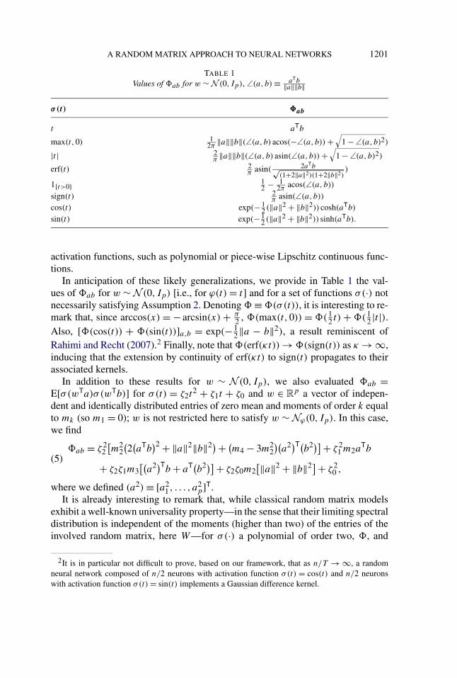
TABLE 1Values of �ab for w ∼ N (0, Ip), ∠(a, b) ≡ aTb
‖a‖‖b‖
σ(t) �ab
t aTb
max(t,0) 12π
‖a‖‖b‖(∠(a, b) acos(−∠(a, b)) +√
1 −∠(a, b)2)
|t | 2π ‖a‖‖b‖(∠(a, b) asin(∠(a, b)) +
√1 −∠(a, b)2)
erf(t) 2π asin( 2aTb√
(1+2‖a‖2)(1+2‖b‖2))
1{t>0} 12 − 1
2πacos(∠(a, b))
sign(t) 2π asin(∠(a, b))
cos(t) exp(− 12 (‖a‖2 + ‖b‖2)) cosh(aTb)
sin(t) exp(− 12 (‖a‖2 + ‖b‖2)) sinh(aTb).
activation functions, such as polynomial or piece-wise Lipschitz continuous func-tions.
In anticipation of these likely generalizations, we provide in Table 1 the val-ues of �ab for w ∼ N (0, Ip) [i.e., for ϕ(t) = t] and for a set of functions σ(·) notnecessarily satisfying Assumption 2. Denoting � ≡ �(σ(t)), it is interesting to re-mark that, since arccos(x) = − arcsin(x) + π
2 , �(max(t,0)) = �(12 t) + �(1
2 |t |).Also, [�(cos(t)) + �(sin(t))]a,b = exp(−1
2‖a − b‖2), a result reminiscent ofRahimi and Recht (2007).2 Finally, note that �(erf(κt)) → �(sign(t)) as κ → ∞,inducing that the extension by continuity of erf(κt) to sign(t) propagates to theirassociated kernels.
In addition to these results for w ∼ N (0, Ip), we also evaluated �ab =E[σ(wTa)σ (wTb)] for σ(t) = ζ2t
2 + ζ1t + ζ0 and w ∈ Rp a vector of indepen-
dent and identically distributed entries of zero mean and moments of order k equalto mk (so m1 = 0); w is not restricted here to satisfy w ∼ Nϕ(0, Ip). In this case,we find
�ab = ζ 22[m2
2(2(aTb)2 + ‖a‖2‖b‖2)+ (m4 − 3m2
2)(
a2)T(b2)]+ ζ 21 m2a
Tb(5)
+ ζ2ζ1m3[(
a2)Tb + aT(b2)]+ ζ2ζ0m2[‖a‖2 + ‖b‖2]+ ζ 2
0 ,
where we defined (a2) ≡ [a21, . . . , a2
p]T.It is already interesting to remark that, while classical random matrix models
exhibit a well-known universality property—in the sense that their limiting spectraldistribution is independent of the moments (higher than two) of the entries of theinvolved random matrix, here W—for σ(·) a polynomial of order two, �, and
2It is in particular not difficult to prove, based on our framework, that as n/T → ∞, a randomneural network composed of n/2 neurons with activation function σ(t) = cos(t) and n/2 neuronswith activation function σ(t) = sin(t) implements a Gaussian difference kernel.
1202 C. LOUART, Z. LIAO AND R. COUILLET
thus μn strongly depend on E[Wkij ] for k = 3,4. We shall see in Section 4 that
this remark has troubling consequences. We will notably infer (and confirm viasimulations) that the studied neural network may provably fail to fulfill a specifictask if the Wij are Bernoulli with zero mean and unit variance but succeed withpossibly high performance if the Wij are standard Gaussian [which is explainedby the disappearance or not of the term (aTb)2 and (a2)T(b2) in (5) if m4 = m2
2].
4. Practical outcomes. We discuss in this section the outcomes of our mainresults in terms of neural network application. The technical discussions on The-orem 1 and Proposition 1 will be made in the course of their respective proofs inSection 5.
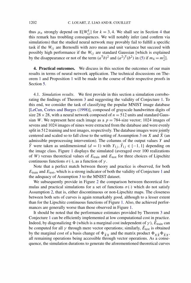
4.1. Simulation results. We first provide in this section a simulation corrobo-rating the findings of Theorem 3 and suggesting the validity of Conjecture 1. Tothis end, we consider the task of classifying the popular MNIST image database[LeCun, Cortes and Burges (1998)], composed of grayscale handwritten digits ofsize 28×28, with a neural network composed of n = 512 units and standard Gaus-sian W . We represent here each image as a p = 784-size vector; 1024 images ofsevens and 1024 images of nines were extracted from the database and were evenlysplit in 512 training and test images, respectively. The database images were jointlycentered and scaled so to fall close to the setting of Assumption 3 on X and X (anadmissible preprocessing intervention). The columns of the output values Y andY were taken as unidimensional (d = 1) with Y1j , Y1j ∈ {−1,1} depending onthe image class. Figure 1 displays the simulated (averaged over 100 realizationsof W ) versus theoretical values of Etrain and Etest for three choices of Lipschitzcontinuous functions σ(·), as a function of γ .
Note that a perfect match between theory and practice is observed, for bothEtrain and Etest, which is a strong indicator of both the validity of Conjecture 1 andthe adequacy of Assumption 3 to the MNIST dataset.
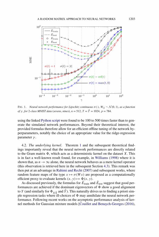
We subsequently provide in Figure 2 the comparison between theoretical for-mulas and practical simulations for a set of functions σ(·) which do not satisfyAssumption 2, that is, either discontinuous or non-Lipschitz maps. The closenessbetween both sets of curves is again remarkably good, although to a lesser extentthan for the Lipschitz continuous functions of Figure 1. Also, the achieved perfor-mances are generally worse than those observed in Figure 1.
It should be noted that the performance estimates provided by Theorem 3 andConjecture 1 can be efficiently implemented at low computational cost in practice.Indeed, by diagonalizing � (which is a marginal cost independent of γ ), Etrain canbe computed for all γ through mere vector operations; similarly, Etest is obtainedby the marginal cost of a basis change of �
XXand the matrix product �
XX�
XX,
all remaining operations being accessible through vector operations. As a conse-quence, the simulation durations to generate the aforementioned theoretical curves
A RANDOM MATRIX APPROACH TO NEURAL NETWORKS 1203
FIG. 1. Neural network performance for Lipschitz continuous σ(·), Wij ∼ N (0,1), as a function
of γ , for 2-class MNIST data (sevens, nines), n = 512, T = T = 1024, p = 784.
using the linked Python script were found to be 100 to 500 times faster than to gen-erate the simulated network performances. Beyond their theoretical interest, theprovided formulas therefore allow for an efficient offline tuning of the network hy-perparameters, notably the choice of an appropriate value for the ridge-regressionparameter γ .
4.2. The underlying kernel. Theorem 1 and the subsequent theoretical find-ings importantly reveal that the neural network performances are directly relatedto the Gram matrix �, which acts as a deterministic kernel on the dataset X. Thisis in fact a well-known result found, for example, in Williams (1998) where it isshown that, as n → ∞ alone, the neural network behaves as a mere kernel operator(this observation is retrieved here in the subsequent Section 4.3). This remark wasthen put at an advantage in Rahimi and Recht (2007) and subsequent works, whererandom feature maps of the type x �→ σ(Wx) are proposed as a computationallyefficient proxy to evaluate kernels (x, y) �→ �(x,y).
As discussed previously, the formulas for Etrain and Etest suggest that good per-formances are achieved if the dominant eigenvectors of � show a good alignmentto Y (and similarly for �
XXand Y ). This naturally drives us to finding a priori sim-
ple regression tasks where ill-choices of � may annihilate the neural network per-formance. Following recent works on the asymptotic performance analysis of ker-nel methods for Gaussian mixture models [Couillet and Benaych-Georges (2016),
1204 C. LOUART, Z. LIAO AND R. COUILLET
FIG. 2. Neural network performance for σ(·) either discontinuous or non-Lipschitz,Wij ∼N (0,1), as a function of γ , for 2-class MNIST data (sevens, nines), n = 512, T = T = 1024,p = 784.
Liao and Couillet (2017), Mai and Couillet (2017)] and [Couillet and Kammoun(2016)], we describe here such a task.
Let x1, . . . , xT/2 ∼ N (0, 1pC1) and xT/2+1, . . . , xT ∼ N (0, 1
pC2) where C1 and
C2 are such that trC1 = trC2, ‖C1‖,‖C2‖ are bounded, and tr(C1 −C2)2 = O(p).
Accordingly, y1, . . . , yT/2+1 = −1 and yT/2+1, . . . , yT = 1. It is proved in theaforementioned articles that, under these conditions, it is theoretically possible, inthe large p,T limit, to classify the data using a kernel least-square support vectormachine (i.e., with a training dataset) or with a kernel spectral clustering method(i.e., in a completely unsupervised manner) with a nontrivial limiting error prob-ability (i.e., neither zero nor one). This scenario has the interesting feature thatxTi xj → 0 almost surely for all i = j while ‖xi‖2 − 1
ptr(1
2C1 + 12C2) → 0, almost
surely, irrespective of the class of xi , thereby allowing for a Taylor expansion ofthe nonlinear kernels as early proposed in El Karoui (2010).
Transposed to our present setting, the aforementioned Taylor expansion allowsfor a consistent approximation � of � by an information-plus-noise (spiked) ran-dom matrix model [see, e.g., Benaych-Georges and Nadakuditi (2012), Loubatonand Vallet (2010)]. In the present Gaussian mixture context, it is shown in Couilletand Benaych-Georges (2016) that data classification is (asymptotically at least)only possible if �ij explicitly contains the quadratic term (xT
i xj )2 [or combina-

A RANDOM MATRIX APPROACH TO NEURAL NETWORKS 1205
tions of (x2i )Txj , (x2
j )Txi , and (x2i )T(x2
j )]. In particular, letting a, b ∼ N (0,Ci)
with i = 1,2, it is easily seen from Table 1 that only max(t,0), |t |, and cos(t) canrealize the task. Indeed, we have the following Taylor expansions around x = 0:
asin(x) = x + O(x3),
sinh(x) = x + O(x3),
acos(x) = π
2− x + O
(x3),
cosh(x) = 1 + x2
2+ O
(x3),
x acos(−x) +√
1 − x2 = 1 + πx
2+ x2
2+ O
(x3),
x asin(x) +√
1 − x2 = 1 + x2
2+ O
(x3),
where only the last three functions [only found in the expression of �ab corre-sponding to σ(t) = max(t,0), |t |, or cos(t)] exhibit a quadratic term.
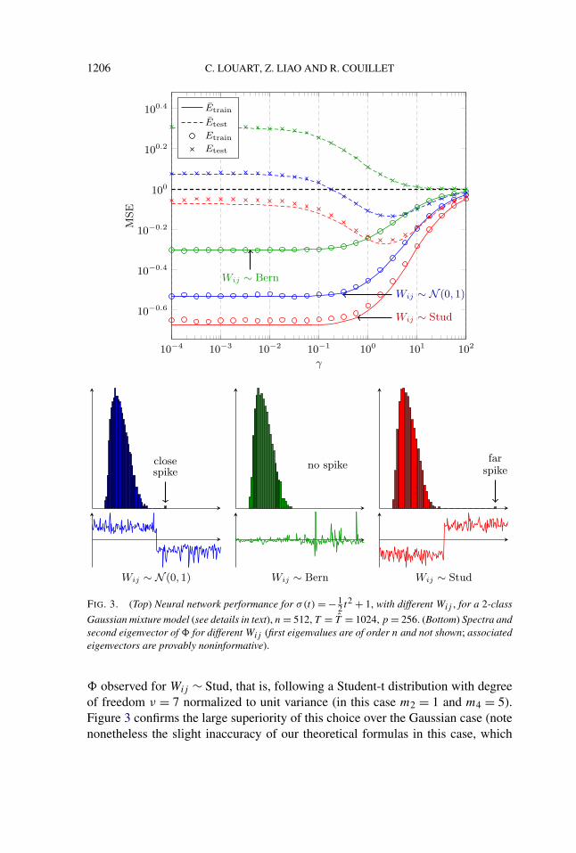
More surprisingly maybe, recalling now equation (5) which considers nonnec-essarily Gaussian Wij with moments mk of order k, a more refined analysis showsthat the aforementioned Gaussian mixture classification task will fail if m3 = 0and m4 = m2
2, so for instance, for Wij ∈ {−1,1} Bernoulli with parameter 12 .
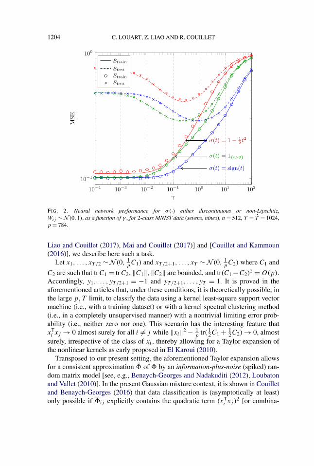
The performance comparison of this scenario is shown in the top part of Fig-ure 3 for σ(t) = −1
2 t2 + 1 and C1 = diag(Ip/2,4Ip/2), C2 = diag(4Ip/2, Ip/2),for Wij ∼ N (0,1) and Wij ∼ Bern [i.e., Bernoulli {(−1, 1
2), (1, 12)}]. The choice
of σ(t) = ζ2t2 + ζ1t + ζ0 with ζ1 = 0 is motivated by Couillet and Benaych-
Georges (2016), Couillet and Kammoun (2016) where it is shown, in a somewhatdifferent setting, that this choice is optimal for class recovery. Note that, whilethe test performances are overall rather weak in this setting, for Wij ∼ N (0,1),Etest drops below one (the amplitude of the Yij ), thereby indicating that nontriv-ial classification is performed. This is not so for the Bernoulli Wij ∼ Bern casewhere Etest is systematically greater than |Yij | = 1. This is theoretically explainedby the fact that, from equation (5), �ij contains structural information about thedata classes through the term 2m2
2(xTi xj )
2 + (m4 − 3m22)(x
2i )T(x2
j ) which induces
an information-plus-noise model for � as long as 2m22 + (m4 − 3m2
2) = 0, that is,m4 = m2
2 [see Couillet and Benaych-Georges (2016) for details]. This is visuallyseen in the bottom part of Figure 3 where the Gaussian scenario presents an iso-lated eigenvalue for � with corresponding structured eigenvector, which is not thecase of the Bernoulli scenario. To complete this discussion, it appears relevant inthe present setting to choose Wij in such a way that m4 − m2
2 is far from zero,thus suggesting the interest of heavy-tailed distributions. To confirm this predic-tion, Figure 3 additionally displays the performance achieved and the spectrum of
1206 C. LOUART, Z. LIAO AND R. COUILLET
FIG. 3. (Top) Neural network performance for σ(t) = − 12 t2 + 1, with different Wij , for a 2-class
Gaussian mixture model (see details in text), n = 512, T = T = 1024, p = 256. (Bottom) Spectra andsecond eigenvector of � for different Wij (first eigenvalues are of order n and not shown; associatedeigenvectors are provably noninformative).
� observed for Wij ∼ Stud, that is, following a Student-t distribution with degreeof freedom ν = 7 normalized to unit variance (in this case m2 = 1 and m4 = 5).Figure 3 confirms the large superiority of this choice over the Gaussian case (notenonetheless the slight inaccuracy of our theoretical formulas in this case, which
A RANDOM MATRIX APPROACH TO NEURAL NETWORKS 1207
is likely due to too small values of p,n,T to accommodate Wij with higher ordermoments, an observation which is confirmed in simulations when letting ν be evensmaller).
4.3. Limiting cases. We have suggested that � contains, in its dominant eigen-modes, all the usable information describing X. In the Gaussian mixture exampleabove, it was notably shown that � may completely fail to contain this information,resulting in the impossibility to perform a classification task, even if one were totake infinitely many neurons in the network. For � containing useful informationabout X, it is intuitive to expect that both infγ Etrain and infγ Etest become smalleras n/T and n/p become large. It is in fact easy to see that, if � is invertible (whichis likely to occur in most cases if lim infn T /p > 1), then
limn→∞ Etrain = 0,
limn→∞ Etest − 1
T
∥∥Y T − �XX
�−1Y T∥∥2F = 0
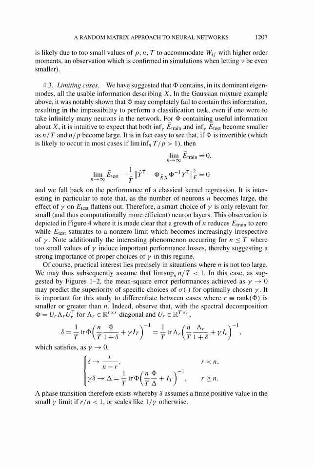
and we fall back on the performance of a classical kernel regression. It is inter-esting in particular to note that, as the number of neurons n becomes large, theeffect of γ on Etest flattens out. Therefore, a smart choice of γ is only relevant forsmall (and thus computationally more efficient) neuron layers. This observation isdepicted in Figure 4 where it is made clear that a growth of n reduces Etrain to zerowhile Etest saturates to a nonzero limit which becomes increasingly irrespectiveof γ . Note additionally the interesting phenomenon occurring for n ≤ T wheretoo small values of γ induce important performance losses, thereby suggesting astrong importance of proper choices of γ in this regime.
Of course, practical interest lies precisely in situations where n is not too large.We may thus subsequently assume that lim supn n/T < 1. In this case, as sug-gested by Figures 1–2, the mean-square error performances achieved as γ → 0may predict the superiority of specific choices of σ(·) for optimally chosen γ . Itis important for this study to differentiate between cases where r ≡ rank(�) issmaller or greater than n. Indeed, observe that, with the spectral decomposition� = Ur�rU
Tr for �r ∈ R
r×r diagonal and Ur ∈ RT ×r ,
δ = 1
Ttr�(
n
T
�
1 + δ+ γ IT
)−1= 1
Ttr�r
(n
T
�r
1 + δ+ γ Ir
)−1,
which satisfies, as γ → 0,⎧⎪⎪⎨⎪⎪⎩
δ → r
n − r, r < n,
γ δ → � = 1
Ttr�(
n
T
�
�+ IT
)−1, r ≥ n.
A phase transition therefore exists whereby δ assumes a finite positive value in thesmall γ limit if r/n < 1, or scales like 1/γ otherwise.
1208 C. LOUART, Z. LIAO AND R. COUILLET
FIG. 4. Neural network performance for growing n (256, 512, 1024, 2048, 4096) as a function ofγ , σ(t) = max(t,0); 2-class MNIST data (sevens, nines), T = T = 1024, p = 784. Limiting (n = ∞)Etest shown in thick black line.
As a consequence, if r < n, as γ → 0, → nT(1 − r
n)� and Q ∼ T
n−rUr ×
�−1r UT
r + 1γVrV
Tr , where Vr ∈ R
T ×(n−r) is any matrix such that [UrVr ] is or-
thogonal, so that Q → UrUTr and Q2 → Ur�
−1r UT
r ; and thus, Etrain →1T
trYVrVTr Y T = 1
T‖YVr‖2
F , which states that the residual training error corre-sponds to the energy of Y not captured by the space spanned by �. Since Etrain isan increasing function of γ , so is Etrain (at least for all large n), and thus 1
T‖YVr‖2
F
corresponds to the lowest achievable asymptotic training error.If instead r > n (which is the most likely outcome in practice), as γ → 0, Q ∼
1γ( nT
��
+ IT )−1 and thus
Etrainγ→0−→ 1
TtrYQ�
[ 1n
tr �Q2�
1 − 1n
tr( �Q�)2 � + IT
]Q�Y T,
where � = nT
��
and Q� = ( nT
��
+ IT )−1.These results suggest that neural networks should be designed both in a way that
reduces the rank of � while maintaining a strong alignment between the dominanteigenvectors of � and the output matrix Y .
Interestingly, if X is assumed as above to be extracted from a Gaussian mixtureand that Y ∈ R
1×T is a classification vector with Y1j ∈ {−1,1}, then the toolsproposed in Couillet and Benaych-Georges (2016) (related to spike random matrix
A RANDOM MATRIX APPROACH TO NEURAL NETWORKS 1209
analysis) allow for an explicit evaluation of the aforementioned limits as n,p,T
grow large. This analysis is however cumbersome and outside the scope of thepresent work.
5. Proof of the main results. In the remainder, we shall use extensively thefollowing notation:
� = σ(WX) =
⎡⎢⎢⎣σ T
1...
σ Tn
⎤⎥⎥⎦ , W =
⎡⎢⎢⎣wT
1...
wTn
⎤⎥⎥⎦
that is, σi = σ(wTi X)T. Also, we shall define �−i ∈ R
(n−1)×T the matrix � withith row removed, and correspondingly
Q−i =(
1
T�T� − 1
Tσiσ
Ti + γ IT
)−1.
Finally, because of exchangeability, it shall often be convenient to work with thegeneric random vector w ∼ Nϕ(0, IT ), the random vector σ distributed as anyof the σi ’s, the random matrix �− distributed as any of the �−i’s, and with therandom matrix Q− distributed as any of the Q−i ’s.
5.1. Concentration results on �. Our first results provide concentration ofmeasure properties on functionals of �. These results unfold from the follow-ing concentration inequality for Lipschitz applications of a Gaussian vector; see,for example, Ledoux (2005), Corollary 2.6, Propositions 1.3, 1.8 or Tao (2012),Theorem 2.1.12. For d ∈ N, consider μ the canonical Gaussian probability on
Rd defined through its density dμ(w) = (2π)− d
2 e− 12 ‖w‖2
and f : Rd → R a λf -Lipschitz function. Then we have the said normal concentration
μ
({∣∣∣∣f −∫
f dμ
∣∣∣∣≥ t
})≤ Ce
−c t2
λ2f ,(6)
where C,c > 0 are independent of d and λf . As a corollary [see, e.g., Ledoux(2005)], for every k ≥ 1,
E[∣∣∣∣f −
∫f dμ
∣∣∣∣k]
≤(
Cλf√c
)k
.
The main approach to the proof of our results, starting with that of the keyLemma 1, is as follows: since Wij = ϕ(Wij ) with Wij ∼ N (0,1) and ϕ Lipschitz,the normal concentration of W transfers to W which further induces a normalconcentration of the random vector σ and the matrix �, thereby implying thatLipschitz functionals of σ or � also concentrate. As pointed out earlier, these
1210 C. LOUART, Z. LIAO AND R. COUILLET
concentration results are used in place for the independence assumptions (and theirmultiple consequences on convergence of random variables) classically exploitedin random matrix theory.
Notation: In all subsequent lemmas and proofs, the letters c, ci,C,Ci > 0 willbe used interchangeably as positive constants independent of the key equation pa-rameters (notably n and t below) and may be reused from line to line. Additionally,the variable ε > 0 will denote any small positive number; the variables c, ci,C,Ci
may depend on ε.We start by recalling the first part of the statement of Lemma 1 and subsequently
providing its proof.
LEMMA 2 (Concentration of quadratic forms). Let Assumptions 1–2 hold. Letalso A ∈ R
T ×T such that ‖A‖ ≤ 1 and, for X ∈ Rp×T and w ∼ Nϕ(0, Ip), define
the random vector σ ≡ σ(wTX)T ∈ RT . Then
P
(∣∣∣∣ 1T σ TAσ − 1
Ttr�A
∣∣∣∣> t
)≤ Ce
− cT
‖X‖2λ2ϕλ2
σmin( t2
t20,t)
for t0 ≡ |σ(0)| + λϕλσ‖X‖√
pT
and C,c > 0 independent of all other parameters.
PROOF. The layout of the proof is as follows: since the application w �→1Tσ TAσ is “quadratic” in w, and thus not Lipschitz (therefore not allowing for
a natural transfer of the concentration of w to 1Tσ TAσ ), we first prove that 1√
T‖σ‖
satisfies a concentration inequality, which provides a high probability O(1) boundon 1√
T‖σ‖. Conditioning on this event, the map w �→ 1√
Tσ TAσ can then be shown
to be Lipschitz (by isolating one of the σ terms for bounding and the other one forretrieving the Lipschitz character) and, up to an appropriate control of concentra-tion results under conditioning, the result is obtained.
Following this plan, we first provide a concentration inequality for ‖σ‖. To thisend, note that the application ψ : Rp → R
T , w �→ σ(ϕ(w)TX)T is Lipschitz withparameter λϕλσ‖X‖ as the combination of the λϕ-Lipschitz function ϕ : w �→ w,the ‖X‖-Lipschitz map R
n → RT , w �→ XTw and the λσ -Lipschitz map R
T →R
T , Y �→ σ(Y ). As a Gaussian vector, w has a normal concentration and so doesψ(w). Since the Euclidean norm R
T →R, Y �→ ‖Y‖ is 1-Lipschitz, we thus haveimmediately by (6)
P
(∣∣∣∣∥∥∥∥ 1√
Tσ(wTX
)∥∥∥∥− E[∥∥∥∥ 1√
Tσ(wTX
)∥∥∥∥]∣∣∣∣≥ t
)≤ Ce
− cT t2
‖X‖2λ2σ λ2
ϕ
for some c,C > 0 independent of all parameters.Finally, using again the Lipschitz character of σ(wTX),∣∣∥∥σ (wTX
)∥∥− ∥∥σ(0)1TT
∥∥∣∣≤ ∥∥σ (wTX)− σ(0)1T
T
∥∥≤ λσ‖w‖ · ‖X‖

A RANDOM MATRIX APPROACH TO NEURAL NETWORKS 1211
so that, by Jensen’s inequality,
E[∥∥∥∥ 1√
Tσ(wTX
)∥∥∥∥]
≤ ∣∣σ(0)∣∣+ λσ E
[1√T
‖w‖]‖X‖
≤ ∣∣σ(0)∣∣+ λσ
√E[
1
T‖w‖2
]‖X‖
with E[‖ϕ(w)‖2] ≤ λ2ϕE[‖w‖2] = pλ2
ϕ [since w ∼ N (0, Ip)]. Letting t0 ≡|σ(0)| + λσλϕ‖X‖
√pT
, we then find
P
(∥∥∥∥ 1√T
σ(wTX
)∥∥∥∥≥ t + t0
)≤ Ce
− cT t2
λ2ϕλ2
σ ‖X‖2,
which, with the remark t ≥ 4t0 ⇒ (t − t0)2 ≥ t2/2, may be equivalently stated as
∀t ≥ 4t0, P
(∥∥∥∥ 1√T
σ(wTX
)∥∥∥∥≥ t
)≤ Ce
− cT t2
2λ2ϕλ2
σ ‖X‖2.(7)
As a side (but important) remark, note that, since
P
(∥∥∥∥ �√T
∥∥∥∥F
≥ t√
T
)= P
(√√√√ n∑i=1
∥∥∥∥ σi√T
∥∥∥∥2≥ t
√T
)
≤ P
(max
1≤i≤n
∥∥∥∥ σi√T
∥∥∥∥≥√
T
nt
)
≤ nP
(∥∥∥∥ σ√T
∥∥∥∥≥√
T
nt
)
the result above implies that
∀t ≥ 4t0, P
(∥∥∥∥ �√T
∥∥∥∥F
≥ t√
T
)≤ Cne
− cT 2t2
2nλ2ϕλ2
σ ‖X‖2
and thus, since ‖ · ‖F ≥ ‖ · ‖, we have
∀t ≥ 4t0, P
(∥∥∥∥ �√T
∥∥∥∥≥ t√
T
)≤ Cne
− cT 2t2
2nλ2ϕλ2
σ ‖X‖2.
Thus, in particular, under the additional Assumption 3, with high probability, theoperator norm of �√
Tcannot exceed a rate
√T .
REMARK 1 (Loss of control of the structure of �). The aforementioned con-trol of ‖�‖ arises from the bound ‖�‖ ≤ ‖�‖F which may be quite loose (byas much as a factor
√T ). Intuitively, under the supplementary Assumption 3, if

1212 C. LOUART, Z. LIAO AND R. COUILLET
E[σ ] = 0, then �√T
is “dominated” by the matrix 1√T
E[σ ]1TT , the operator norm of
which is indeed of order√
n and the bound is tight. If σ(t) = t and E[Wij ] = 0, wehowever know that ‖ �√
T‖ = O(1) [Bai and Silverstein (1998)]. One is tempted to
believe that, more generally, if E[σ ] = 0, then ‖ �√T‖ should remain of this order.
And, if instead E[σ ] = 0, the contribution of 1√T
E[σ ]1TT should merely engender
a single large amplitude isolate singular value in the spectrum of �√T
and the othersingular values remain of order O(1). These intuitions are not captured by ourconcentration of measure approach.
Since � = σ(WX) is an entry-wise operation, concentration results with re-spect to the Frobenius norm are natural, where with respect to the operator normare hardly accessible.
Back to our present considerations, let us define the probability space AK ={w,‖σ(wTX)‖ ≤ K
√T }. Conditioning the random variable of interest in
Lemma 2 with respect to AK and its complementary AcK , for some K ≥ 4t0,
gives
P
(∣∣∣∣ 1T σ(wTX
)Aσ(wTX
)T − 1
Ttr�A
∣∣∣∣> t
)
≤ P
({∣∣∣∣ 1T σ(wTX
)Aσ(wTX
)T − 1
Ttr�A
∣∣∣∣> t
},AK
)+ P(Ac
K
).
We can already bound P(AcK) thanks to (7). As for the first right-hand side term,
note that on the set {σ(wTX),w ∈ AK}, the function f : RT → R : σ �→ σ TAσ isK
√T -Lipschitz. This is because, for all σ,σ + h ∈ {σ(wTX),w ∈ AK},∥∥f (σ + h) − f (σ)
∥∥= ∥∥hTAσ + (σ + h)TAh∥∥≤ K
√T ‖h‖.
Since conditioning does not allow for a straightforward application of (6), weconsider instead f , a K
√T -Lipschitz continuation to R
T of fAK, the restric-
tion of f to AK , such that all the radial derivative of f are constant in the set{σ,‖σ‖ ≥ K
√T }. We may thus now apply (6) and our previous results to obtain
P(∣∣f (σ (wTX
))− E[f(σ(wTX
))]∣∣≥ KT t)≤ e
− cT t2
‖X‖2λ2σ λ2
ϕ .
Therefore,
P({∣∣f (σ (wTX
))− E[f(σ(wTX
))]∣∣≥ KT t},AK
)= P({∣∣f (σ (wTX
))− E[f(σ(wTX
))]∣∣≥ KT t},AK
)
≤ P(∣∣f (σ (wTX
))− E[f(σ(wTX
))]∣∣≥ KT t)≤ e
− cT t2
‖X‖2λ2σ λ2
ϕ .
A RANDOM MATRIX APPROACH TO NEURAL NETWORKS 1213
Our next step is then to bound the difference � = |E[f (σ (wTX))] −E[f (σ(wTX))]|. Since f and f are equal on {σ,‖σ‖ ≤ K
√T },
� ≤∫‖σ‖≥K
√T
(∣∣f (σ)∣∣+ ∣∣f (σ )
∣∣)dμσ (σ ),
where μσ is the law of σ(wTX). Since ‖A‖ ≤ 1, for ‖σ‖ ≥ K√
T , max(|f (σ)|,|f (σ )|) ≤ ‖σ‖2, and thus
� ≤ 2∫‖σ‖≥K
√T
‖σ‖2 dμσ = 2∫‖σ‖≥K
√T
∫ ∞t=0
1‖σ‖2≥t dt dμσ
= 2∫ ∞t=0
P({‖σ‖2 ≥ t
},Ac
K
)dt
≤ 2∫ K2T
t=0P(Ac
K
)dt + 2
∫ ∞t=K2T
P(∥∥σ (wTX
)∥∥2 ≥ t)dt
≤ 2P(Ac
K
)K2T + 2
∫ ∞t=K2T
Ce− ct
2λ2ϕλ2
σ ‖X‖2dt
≤ 2CT K2e− cT K2
2λ2ϕλ2
σ ‖X‖2 + 2Cλ2ϕλ2
σ‖X‖2
ce− cT K2
2λ2ϕλ2
σ ‖X‖2
≤ 6C
cλ2
ϕλ2σ‖X‖2,
where in last inequality we used the fact that for x ∈ R, xe−x ≤ e−1 ≤ 1, and
K ≥ 4t0 ≥ 4λσλϕ‖X‖√
pT
. As a consequence,
P({∣∣f (σ (wTX
))− E[f(σ(wTX
))]∣∣≥ KT t + �},AK
)≤ Ce− cT t2
‖X‖2λ2ϕλ2
σ
so that, with the same remark as before, for t ≥ 4�KT
,
P({∣∣f (σ (wTX
))− E[f(σ(wTX
))]∣∣≥ KT t},AK
)≤ Ce− cT t2
2‖X‖2λ2ϕλ2
σ .
To avoid the condition t ≥ 4�KT
, we use the fact that, probabilities being lower thanone, it suffices to replace C by λC with λ ≥ 1 such that
λCe−c T t2
2‖X‖2λ2ϕλ2
σ ≥ 1 for t ≤ 4�
KT.
The above inequality holds if we take for instance λ = 1C
e18C2
c since then t ≤4�KT
≤ 24Cλ2ϕλ2
σ ‖X‖2
cKT≤ 6Cλϕλσ ‖X‖
c√
pT(using successively � ≥ 6C
cλ2
ϕλ2σ‖X‖2 and K ≥
4λσλϕ‖X‖√
pT
), and thus
λCe− cT t2
2‖X‖2λ2ϕλ2
σ ≥ λCe− 18C2
cp ≥ λCe− 18C2c ≥ 1.

1214 C. LOUART, Z. LIAO AND R. COUILLET
Therefore, setting λ = max(1, 1C
eC′2c
2 ), we get for every t > 0
P({∣∣f (σ
(wTX
))− E[f(σ(wTX)
)]∣∣≥ KT t},AK
)
≤ λCe− cT t2
2‖X‖2λ2ϕλ2
σ ,
which, together with the inequality P(AcK) ≤ Ce
− cT K2
2λ2ϕλ2
σ ‖X‖2 , gives
P(∣∣f (σ (wTX
))− E[f(σ(wTX
))]∣∣≥ KT t)
≤ λCe− T ct2
2‖X‖2λ2ϕλ2
σ + Ce− cT K2
2λ2ϕλ2
σ ‖X‖2.
We then conclude
P
(∣∣∣∣ 1T σ(wTX
)Aσ(wTX
)T − 1
Ttr(�A)
∣∣∣∣≥ t
)
≤ (λ + 1)Ce− cT
2‖X‖2λ2ϕλ2
σmin(t2/K2,K2)
and, with K = max(4t0,√
t),
P
(∣∣∣∣ 1T σ(wTX
)Aσ(wTX
)T − 1
Ttr(�A)
∣∣∣∣≥ t
)≤ (λ + 1)Ce
−cT min( t2
16t20,t)
2‖X‖2λ2ϕλ2
σ .
Indeed, if 4t0 ≤ √t then min(t2/K2,K2) = t , while if 4t0 ≥ √
t then min(t2/K2,
K2) = min(t2/16t20 ,16t2
0 ) = t2/16t20 . �
As a corollary of Lemma 2, we have the following control of the moments of1Tσ TAσ .
COROLLARY 1 (Moments of quadratic forms). Let Assumptions 1–2 hold. Forw ∼ Nϕ(0, Ip), σ ≡ σ(wTX)T ∈R
T , A ∈ RT ×T such that ‖A‖ ≤ 1, and k ∈ N,
E[∣∣∣∣ 1T σ TAσ − 1
Ttr�A
∣∣∣∣k]
≤ C1
(t0η√
T
)k
+ C2
(η2
T
)k
with t0 = |σ(0)| + λσλϕ‖X‖√
pT
, η = ‖X‖λσλϕ , and C1,C2 > 0 independent ofthe other parameters. In particular, under the additional Assumption 3,
E[∣∣∣∣ 1T σ TAσ − 1
Ttr�A
∣∣∣∣k]
≤ C
nk/2 .
A RANDOM MATRIX APPROACH TO NEURAL NETWORKS 1215
PROOF. We use the fact that, for a nonnegative random variable Y , E[Y ] =∫∞0 P(Y > t) dt , so that
E[∣∣∣∣ 1T σ TAσ − 1
Ttr�A
∣∣∣∣k]
=∫ ∞
0P
(∣∣∣∣ 1T σ TAσ − 1
Ttr�A
∣∣∣∣k > u
)du
=∫ ∞
0kvk−1P
(∣∣∣∣ 1T σ TAσ − 1
Ttr�A
∣∣∣∣> v
)dv
≤∫ ∞
0kvk−1Ce
− cT
η2 min( v2
t20,v)
dv
≤∫ t0
0kvk−1Ce
− cT v2
t20 η2dv +
∫ ∞t0
kvk−1Ce− cT v
η2 dv
≤∫ ∞
0kvk−1Ce
− cT v2
t20 η2dv +
∫ ∞0
kvk−1Ce− cT v
η2 dv
=(
t0η√cT
)k ∫ ∞0
ktk−1Ce−t2dt +
(η2
cT
)k ∫ ∞0
ktk−1Ce−t dt,
which, along with the boundedness of the integrals, concludes the proof. �
Beyond concentration results on functions of the vector σ , we also have thefollowing convenient property for functions of the matrix �.
LEMMA 3 (Lipschitz functions of �). Let f : Rn×T → R be a λf -Lipschitzfunction with respect to the Froebnius norm. Then, under Assumptions 1–2,
P
(∣∣∣∣f(
�√T
)− Ef
(�√T
)∣∣∣∣> t
)≤ Ce
− cT t2
λ2σ λ2
ϕλ2f
‖X‖2
for some C,c > 0. In particular, under the additional Assumption 3,
P
(∣∣∣∣f(
�√T
)− Ef
(�√T
)∣∣∣∣> t
)≤ Ce−cT t2
.
PROOF. Denoting W = ϕ(W ), since vec(W ) ≡ [W11, . . . , Wnp] is a Gaussianvector, by the normal concentration of Gaussian vectors, for g a λg-Lipschitz func-tion of W with respect to the Frobenius norm [i.e., the Euclidean norm of vec(W)],by (6),
P(∣∣g(W) − E
[g(W)
]∣∣> t)= P
(∣∣g(ϕ(W ))− E
[g(ϕ(W )
)]∣∣> t)≤ Ce
− ct2
λ2gλ2
ϕ
1216 C. LOUART, Z. LIAO AND R. COUILLET
for some C,c > 0. Let us consider in particular g : W �→ f (�/√
T ) and remarkthat
∣∣g(W + H) − g(W)∣∣= ∣∣∣∣f
(σ((W + H)X)√
T
)− f
(σ(WX)√
T
)∣∣∣∣≤ λf√
T
∥∥σ ((W + H)X)− σ(WX)
∥∥F
≤ λf λσ√T
‖HX‖F
= λf λσ√T
√trHXXTH T
≤ λf λσ√T
√∥∥XXT∥∥‖H‖F
concluding the proof. �
A first corollary of Lemma 3 is the concentration of the Stieltjes’ transform1T
tr( 1T�T� − zIT )−1 of μn, the empirical spectral measure of 1
T�T�, for all
z ∈C \R+ (so in particular, for z = −γ , γ > 0).
COROLLARY 2 (Concentration of the Stieltjes’ transform of μn). Under As-sumptions 1–2, for z ∈ C \R+,
P
(∣∣∣∣ 1T tr(
1
T�T� − zIT
)−1− E[
1
Ttr(
1
T�T� − zIT
)−1]∣∣∣∣> t
)
≤ Ce− c dist(z,R+)2T t2
λ2σ λ2
ϕ‖X‖2
for some C,c > 0, where dist(z,R+) is the Hausdorff set distance. In particular,for z = −γ , γ > 0, and under the additional Assumption 3,
P
(∣∣∣∣ 1T trQ − 1
Ttr E[Q]
∣∣∣∣> t
)≤ Ce−cnt2
.
PROOF. We can apply Lemma 3 for f : R �→ 1T
tr(RTR − zIT )−1, since wehave∣∣f (R + H) − f (R)
∣∣=∣∣∣∣ 1T tr
((R + H)T(R + H) − zIT
)−1((R + H)TH + H TR
)(RTR − zIT
)−1∣∣∣∣
≤∣∣∣∣ 1T tr
((R + H)T(R + H) − zIT
)−1(R + H)TH
(RTR − zIT
)−1∣∣∣∣
A RANDOM MATRIX APPROACH TO NEURAL NETWORKS 1217
+∣∣∣∣ 1T tr
((R + H)T(R + H) − zIT
)−1H TR
(RTR − zIT
)−1∣∣∣∣
≤ 2‖H‖dist(z,R+)
32
≤ 2‖H‖F
dist(z,R+)32
,
where, for the second to last inequality, we successively used the relations| trAB| ≤ √
trAAT√
trBBT, | trCD| ≤ ‖D‖ trC for nonnegative definite C,and ‖(RTR − zIT )−1‖ ≤ dist(z,R+)−1, ‖(RTR − zIT )−1RTR‖ ≤ 1, ‖(RTR −zIT )−1RT‖ = ‖(RTR − zIT )−1RTR(RTR − zIT )−1‖ 1
2 ≤ ‖(RTR − zIT )−1RT ×R‖ 1
2 ‖(RTR − zIT )−1‖ 12 ≤ dist(z,R+)− 1
2 , for z ∈ C\R+, and finally ‖ · ‖ ≤ ‖ · ‖F .�
Lemma 3 also allows for an important application of Lemma 2 as follows.
LEMMA 4 (Concentration of 1Tσ TQ−σ ). Let Assumptions 1–3 hold and write
WT = [w1, . . . ,wn]. Define σ ≡ σ(wT1X)T ∈ R
T and, for WT− = [w2, . . . ,wn] and�− = σ(W−X), let Q− = ( 1
T�T−�− + γ IT )−1. Then, for A,B ∈R
T ×T such that‖A‖,‖B‖ ≤ 1
P
(∣∣∣∣ 1T σ TAQ−Bσ − 1
Ttr�AE[Q−]B
∣∣∣∣> t
)≤ Ce−cnmin(t2,t)
for some C,c > 0 independent of the other parameters.
PROOF. Let f : R �→ 1Tσ TA(RTR + γ IT )−1Bσ . Reproducing the proof of
Corollary 2, conditionally to 1T‖σ‖2 ≤ K for any arbitrary large enough K > 0,
it appears that f is Lipschitz with parameter of order O(1). Along with (7) andAssumption 3, this thus ensures that
P
(∣∣∣∣ 1T σ TAQ−Bσ − 1
Tσ TAE[Q−]Bσ
∣∣∣∣> t
)
≤ P
(∣∣∣∣ 1T σ TAQ−Bσ − 1
Tσ TAE[Q−]Bσ
∣∣∣∣> t,‖σ‖2
T≤ K
)
+ P
(‖σ‖2
T> K
)≤ Ce−cnt2
for some C,c > 0. We may then apply Lemma 1 on the bounded norm matrixAE[Q−]B to further find that
P
(∣∣∣∣ 1T σ TAQ−Bσ − 1
Ttr�AE[Q−]B
∣∣∣∣> t
)
≤ P
(∣∣∣∣ 1T σ TAQ−Bσ − 1
Tσ TAE[Q−]Bσ
∣∣∣∣> t
2
)
1218 C. LOUART, Z. LIAO AND R. COUILLET
+ P
(∣∣∣∣ 1T σ TAE[Q−]Bσ − 1
Ttr�AE[Q−]B
∣∣∣∣> t
2
)
≤ C′e−c′nmin(t2,t),
which concludes the proof. �
As a further corollary of Lemma 3, we have the following concentration resulton the training mean-square error of the neural network under study.
COROLLARY 3 (Concentration of the mean-square error). Under Assumptions1–3,
P
(∣∣∣∣ 1T trY TYQ2 − 1
TtrY TYE
[Q2]∣∣∣∣> t
)≤ Ce−cnt2
for some C,c > 0 independent of the other parameters.
PROOF. We apply Lemma 3 to the mapping f : R �→ 1T
trY TY(RTR +γ IT )−2. Denoting Q = (RTR +γ IT )−1 and QH = ((R +H)T(R +H)+γ IT )−1,remark indeed that∣∣f (R + H) − f (R)
∣∣=∣∣∣∣ 1T trY TY
((QH )2 − Q2)∣∣∣∣
≤∣∣∣∣ 1T trY TY
(QH − Q
)QH
∣∣∣∣+∣∣∣∣ 1T trY TYQ
(QH − Q
)∣∣∣∣=∣∣∣∣ 1T trY TYQH ((R + H)T(R + H) − RTR
)QQH
∣∣∣∣+∣∣∣∣ 1T trY TYQQH ((R + H)T(R + H) − RTR
)Q
∣∣∣∣≤∣∣∣∣ 1T trY TYQH(R + H)THQQH
∣∣∣∣+∣∣∣∣ 1T trY TYQHH TRQQH
∣∣∣∣+∣∣∣∣ 1T trY TYQQH(R + H)TRQ
∣∣∣∣+∣∣∣∣ 1T trY TYQQHH TRQ
∣∣∣∣.As ‖QH(R + H)T‖ =
√‖QH(R + H)T(R + H)QH‖ and ‖RQ‖ =√‖QRTRQ‖
are bounded and 1T
trY TY is also bounded by Assumption 3, this implies∣∣f (R + H) − f (R)∣∣≤ C‖H‖ ≤ C‖H‖F
A RANDOM MATRIX APPROACH TO NEURAL NETWORKS 1219
for some C > 0. The function f is thus Lipschitz with parameter independent of n,which allows us to conclude using Lemma 3. �
The aforementioned concentration results are the building blocks of the proofsof Theorem 1–3 which, under all Assumptions 1–3, are established using standardrandom matrix approaches.
5.2. Asymptotic equivalents.
5.2.1. First equivalent for E[Q]. This section is dedicated to a first character-ization of E[Q], in the “simultaneously large” n,p,T regime. This preliminarystep is classical in studying resolvents in random matrix theory as the direct com-parison of E[Q] to Q with the implicit δ may be cumbersome. To this end, let usthus define the intermediary deterministic matrix
Q =(
n
T
�
1 + α+ γ IT
)−1
with α ≡ 1T
tr�E[Q−], where we recall that Q− is a random matrix distributed as,say, ( 1
T�T� − 1
Tσ1σ
T1 + γ IT )−1.
First note that, since 1T
tr� = E[ 1T‖σ‖2] and, from (7) and Assumption 3,
P( 1T‖σ‖2 > t) ≤ Ce−cnt2
for all large t , we find that 1T
tr� = ∫∞0 t2P( 1
T‖σ‖2 >
t)dt ≤ C′ for some constant C′. Thus, α ≤ ‖E[Q−]‖ 1T
tr� ≤ C′γ
is uniformlybounded.
We will show here that ‖E[Q] − Q‖ → 0 as n → ∞ in the regime of As-sumption 3. As the proof steps are somewhat classical, we defer to the Appendixsome classical intermediary lemmas (Lemmas 5–7). Using the resolvent identity,Lemma 5, we start by writing
E[Q] − Q = E[Q
(n
T
�
1 + α− 1
T�T�
)]Q
= E[Q] n
T
�
1 + αQ − E
[Q
1
T�T�
]Q
= E[Q] n
T
�
1 + αQ − 1
T
n∑i=1
E[Qσiσ
Ti
]Q,
which, from Lemma 6, gives for Q−i = ( 1T�T� − 1
Tσiσ
Ti + γ IT )−1,
E[Q] − Q
= E[Q] n
T
�
1 + αQ − 1
T
n∑i=1
E[Q−i
σiσTi
1 + 1Tσ T
i Q−iσi
]Q
1220 C. LOUART, Z. LIAO AND R. COUILLET
= E[Q] n
T
�
1 + αQ − 1
1 + α
1
T
n∑i=1
E[Q−iσiσ
Ti
]Q
+ 1
T
n∑i=1
E[Q−iσiσ
Ti ( 1
Tσ T
i Q−iσi − α)
(1 + α)(1 + 1Tσ T
i Q−iσi)
]Q.
Note now, from the independence of Q−i and σiσTi , that the second right-hand
side expectation is simply E[Q−i]�. Also, exploiting Lemma 6 in reverse on therightmost term, this gives
E[Q] − Q = 1
T
n∑i=1
E[Q − Q−i]�1 + α
Q
(8)
+ 1
1 + α
1
T
n∑i=1
E[Qσiσ
Ti Q
(1
Tσ T
i Q−iσi − α
)].
It is convenient at this point to note that, since E[Q] − Q is symmetric, we maywrite
E[Q] − Q = 1
2
1
1 + α
(1
T
n∑i=1
(E[Q − Q−i]�Q + Q�E[Q − Q−i])
(9)
+ 1
T
n∑i=1
E[(
QσiσTi Q + Qσiσ
Ti Q)( 1
Tσ T
i Q−iσi − α
)]).
We study the two right-hand side terms of (9) independently.For the first term, since Q − Q−i = −Q 1
Tσiσ
Ti Q−i ,
1
T
n∑i=1
E[Q − Q−i]�1 + α
Q = 1
1 + α
1
TE
[Q
1
T
n∑i=1
σiσTi Q−i
]�Q
= 1
1 + α
1
TE
[Q
1
T
n∑i=1
σiσTi Q
(1 + 1
Tσ T
i Q−iσi
)]�Q,
where we used again Lemma 6 in reverse. Denoting D = diag({1 + 1Tσ T
i ×Q−iσi}ni=1), this can be compactly written:
1
T
n∑i=1
E[Q − Q−i]�1 + α
Q = 1
1 + α
1
TE[Q
1
T�TD�Q
]�Q.
Note at this point that, from Lemma 7, ‖�Q‖ ≤ (1 + α)Tn
and
∥∥∥∥Q 1√T
�T∥∥∥∥=√∥∥∥∥Q 1
T�T�Q
∥∥∥∥≤ γ − 12 .
A RANDOM MATRIX APPROACH TO NEURAL NETWORKS 1221
Besides, by Lemma 4 and the union bound,
P(
max1≤i≤n
Dii > 1 + α + t)
≤ Cne−cnmin(t2,t)
for some C,c > 0, so in particular, recalling that α ≤ C′ for some constant C′ > 0,
E[
max1≤i≤n
Dii
]=∫ 2(1+C′)
0P(
max1≤i≤n
Dii > t)dt +
∫ ∞2(1+C′)
P(
max1≤i≤n
Dii > t)dt
≤ 2(1 + C′)+ ∫ ∞
2(1+C′)Cne−cnmin((t−(1+C′))2,t−(1+C′)) dt
= 2(1 + C′)+ ∫ ∞
1+C′Cne−cnt dt
= 2(1 + C′)+ e−Cn(1+C′) = O(1).
As a consequence of all the above (and of the boundedness of α), we have that, forsome c > 0,
1
T
∥∥∥∥E[Q
1
T�TD�Q
]�Q
∥∥∥∥≤ c
n.(10)
Let us now consider the second right-hand side term of (9). Using the rela-tion abT + baT � aaT + bbT in the order of Hermitian matrices [which unfoldsfrom (a − b)(a − b)T � 0], we have, with a = T
14 Qσi(
1Tσ T
i Q−iσi − α) and
b = T − 14 Qσi ,
1
T
n∑i=1
E[(
QσiσTi Q + Qσiσ
TQ)( 1
Tσ T
i Q−iσi − α
)]
� 1√T
n∑i=1
E[Qσiσ
Ti Q
(1
Tσ T
i Q−iσi − α
)2]+ 1
T√
T
n∑i=1
E[Qσiσ
Ti Q]
= √T E[Q
1
T�TD2
2�Q
]+ n
T√
TQ�Q,
where D2 = diag({ 1Tσ T
i Q−iσi − α}ni=1). Of course, since we also have −aaT −bbT � abT + baT [from (a + b)(a + b)T � 0], we have symmetrically
1
T
n∑i=1
E[(
QσiσTi Q + Qσiσ
TQ)( 1
Tσ T
i Q−iσi − α
)]
� −√T E[Q
1
T�TD2
2�Q
]− n
T√
TQ�Q.

1222 C. LOUART, Z. LIAO AND R. COUILLET
But from Lemma 4,
P(‖D2‖ > tnε− 1
2)= P
(max
1≤i≤n
∣∣∣∣ 1T σ Ti Q−iσi − α
∣∣∣∣> tnε− 12
)
≤ Cne−cmin(n2εt2,n12 +ε
t)
so that, with a similar reasoning as in the proof of Corollary 1,∥∥∥∥√T E
[Q
1
T�TD2
2�Q
]∥∥∥∥≤ √T E[‖D2‖2]≤ Cnε′− 1
2 ,
where we additionally used ‖Q�‖ ≤ √T in the first inequality.
Since in addition ‖ n
T√
TQ�Q‖ ≤ Cn− 1
2 , this gives
∥∥∥∥∥ 1
T
n∑i=1
E[(
QσiσTi Q + Qσiσ
Ti Q)( 1
Tσ T
i Q−iσi − α
)]∥∥∥∥∥≤ Cnε− 12 .
Together with (9), we thus conclude that
∥∥E[Q] − Q∥∥≤ Cnε− 1
2 .
Note in passing that we proved that
∥∥E[Q − Q−]∥∥= T
n
∥∥∥∥∥ 1
T
n∑i=1
E[Q − Q−i]∥∥∥∥∥=∥∥∥∥1
nE[Q
1
T�TD�Q
]∥∥∥∥≤ c
n,
where the first equality holds by exchangeability arguments.In particular,
α = 1
Ttr�E[Q−] = 1
Ttr�E[Q] + 1
Ttr�(E[Q−] − E[Q]),
where | 1T
tr�(E[Q−] − E[Q])| ≤ cn
. And thus, by the previous result,
∣∣∣∣α − 1
Ttr�Q
∣∣∣∣≤ Cn− 12 +ε 1
Ttr�.
We have proved in the beginning of the section that 1T
tr� is bounded and thus wefinally conclude that
∥∥∥∥α − 1
Ttr�Q
∥∥∥∥≤ Cnε− 12 .
A RANDOM MATRIX APPROACH TO NEURAL NETWORKS 1223
5.2.2. Second equivalent for E[Q]. In this section, we show that E[Q] can beapproximated by the matrix Q, which we recall is defined as
Q =(
n
T
�
1 + δ+ γ IT
)−1,
where δ > 0 is the unique positive solution to δ = 1T
tr�Q. The fact that δ > 0 iswell defined is quite standard and has already been proved several times for moreelaborate models. Following the ideas of Couillet, Hoydis and Debbah (2012), wemay for instance use the framework of so-called standard interference functions[Yates (1995)] which claims that, if a map f : [0,∞) → (0,∞), x �→ f (x), satis-fies x ≥ x′ ⇒ f (x) ≥ f (x′), ∀a > 1, af (x) > f (ax) and there exists x0 such thatx0 ≥ f (x0), then f has a unique fixed point Yates (1995), Theorem 2. It is easilyshown that δ �→ 1
Ttr�Q is such a map, so that δ exists and is unique.
To compare Q and Q, using the resolvent identity, Lemma 5, we start by writing
Q − Q = (α − δ)Qn
T
�
(1 + α)(1 + δ)Q
from which
|α − δ| =∣∣∣∣ 1T tr�
(E[Q−] − Q
)∣∣∣∣≤∣∣∣∣ 1T tr�(Q − Q)
∣∣∣∣+ cn− 12 +ε
= |α − δ| 1
Ttr
�Q nT�Q
(1 + α)(1 + δ)+ cn− 1
2 +ε,
which implies that
|α − δ|(
1 − 1
Ttr
�Q nT�Q
(1 + α)(1 + δ)
)≤ cn− 1
2 +ε.
It thus remains to show that
lim supn
1
Ttr
�Q nT�Q
(1 + α)(1 + δ)< 1
to prove that |α − δ| ≤ cnε− 12 . To this end, note that, by Cauchy–Schwarz’s in-
equality,
1
Ttr
�Q nT�Q
(1 + α)(1 + δ)≤√
n
T (1 + δ)2
1
Ttr�2Q2 · n
T (1 + α)2
1
Ttr�2Q2
so that it is sufficient to bound the limsup of both terms under the square rootstrictly by one. Next, remark that
δ = 1
Ttr�Q = 1
Ttr�Q2Q−1 = n(1 + δ)
T (1 + δ)2
1
Ttr�2Q2 + γ
1
Ttr�Q2.

1224 C. LOUART, Z. LIAO AND R. COUILLET
In particular,
n
T (1 + δ)2
1
Ttr�2Q2 =
δ nT (1+δ)2
1T
tr�2Q2
(1 + δ) nT (1+δ)2
1T
tr�2Q2 + γ 1T
tr�Q2≤ δ
1 + δ.
But at the same time, since ‖( nT� + γ IT )−1‖ ≤ γ −1,
δ ≤ 1
γ Ttr�
the limsup of which is bounded. We thus conclude that
lim supn
n
T (1 + δ)2
1
Ttr�2Q2 < 1.(11)
Similarly, α, which is known to be bounded, satisfies
α = (1 + α)n
T (1 + α)2
1
Ttr�2Q2 + γ
1
Ttr�Q2 + O
(nε− 1
2)
and we thus have also
lim supn
n
T (1 + α)2
1
Ttr�2Q2 < 1,
which completes to prove that |α − δ| ≤ cnε− 12 .
As a consequence of all this,
‖Q − Q‖ = |α − δ| ·∥∥∥∥ Q n
T�Q
(1 + α)(1 + δ)
∥∥∥∥≤ cn− 12 +ε
and we have thus proved that ‖E[Q] − Q‖ ≤ cn− 12 +ε for some c > 0.
From this result, along with Corollary 2, we now have that
P
(∣∣∣∣ 1T trQ − 1
Ttr Q∣∣∣∣> t
)
≤ P
(∣∣∣∣ 1T trQ − 1
Ttr E[Q]
∣∣∣∣> t −∣∣∣∣ 1T tr E[Q] − 1
Ttr Q∣∣∣∣)
≤ C′e−c′n(t−cn− 1
2 +ε) ≤ C′e− 1
2 c′nt
for all large n. As a consequence, for all γ > 0, 1T
trQ− 1T
tr Q → 0 almost surely.As such, the difference mμn − mμn of Stieltjes’ transforms mμn : C \ R
+ → C,z �→ 1
Ttr( 1
T�T� − zIT )−1 and mμn : C \ R
+ → C, z �→ 1T
tr( nT
�1+δz
− zIT )−1
[with δz the unique Stieltjes’ transform solution to δz = 1T
tr�( nT
�1+δz
− zIT )−1]
converges to zero for each z in a subset of C \ R+ having at least one accumu-
lation point (namely R−), almost surely so [i.e., on a probability set Az with
A RANDOM MATRIX APPROACH TO NEURAL NETWORKS 1225
P(Az) = 1]. Thus, letting {zk}∞k=1 be a converging sequence strictly included inR
−, on the probability one space A =⋂∞k=1 Ak , mμn(zk) − mμn(zk) → 0 for all
k. Now, mμn is complex analytic on C \ R+ and bounded on all compact sub-
sets of C \ R+. Besides, it was shown in Silverstein and Bai (1995), Silverstein
and Choi (1995) that the function mμn is well defined, complex analytic andbounded on all compact subsets of C \R+. As a result, on A, mμn − mμn is com-plex analytic, bounded on all compact subsets of C \ R
+ and converges to zeroon a subset admitting at least one accumulation point. Thus, by Vitali’s conver-gence theorem [Titchmarsh (1939)], with probability one, mμn − mμn convergesto zero everywhere on C \ R+. This implies, by Bai and Silverstein (2010), The-orem B.9, that μn − μn → 0, vaguely as a signed finite measure, with prob-ability one, and since μn is a probability measure [again from the results ofSilverstein and Bai (1995), Silverstein and Choi (1995)], we have thus provedTheorem 2.
5.2.3. Asymptotic equivalent for E[QAQ], where A is either � or symmet-ric of bounded norm. The evaluation of the second-order statistics of the neuralnetwork under study requires, beside E[Q], to evaluate the more involved formE[QAQ], where A is a symmetric matrix either equal to � or of bounded norm(so in particular ‖QA‖ is bounded). To evaluate this quantity, first write
E[QAQ]= E[QAQ] + E
[(Q − Q)AQ
]= E[QAQ] + E
[Q
(n
T
�
1 + δ− 1
T�T�
)QAQ
]
= E[QAQ] + n
T
1
1 + δE[Q�QAQ] − 1
T
n∑i=1
E[Qσiσ
Ti QAQ
].
Of course, since QAQ is symmetric, we may write
E[QAQ] = 1
2
(E[QAQ + QAQ] + n
T
1
1 + δE[Q�QAQ + QAQ�Q]
− 1
T
n∑i=1
E[Qσiσ
Ti QAQ + QAQσiσ
Ti Q])
,
which will reveal more practical to handle.
First note that, since ‖E[Q] − Q‖ ≤ Cnε− 12 and A is such that ‖QA‖ is
bounded, ‖E[QAQ]−QAQ‖ ≤ ‖QA‖‖E[Q]−Q‖ ≤ C ′nε− 12 , which provides an
estimate for the first expectation. We next evaluate the last right-hand side expecta-tion above. With the same notation as previously, from exchangeability arguments
1226 C. LOUART, Z. LIAO AND R. COUILLET
and using Q = Q− − Q 1Tσσ TQ−, observe that
1
T
n∑i=1
E[Qσiσ
Ti QAQ
]= n
TE[Qσσ TQAQ
]
= n
TE[Q−σσ TQAQ
1 + 1Tσ TQ−σ
]
= n
T
1
1 + δE[Q−σσ TQAQ
]
+ n
T
1
1 + δE[Q−σσ TQAQ
δ − 1Tσ TQ−σ
1 + 1Tσ TQ−σ
],
which, reusing Q = Q− − Q 1Tσσ TQ−, is further decomposed as
1
T
n∑i=1
E[Qσiσ
Ti QAQ
]
= n
T
1
1 + δE[Q−σσ TQAQ−
]− n
T 2
1
1 + δE[Q−σσ TQAQ−σσ TQ−
1 + 1Tσ TQ−σ
]
+ n
TE[Q−σσ TQAQ−
δ − 1Tσ TQ−σ
(1 + δ)(1 + 1Tσ TQ−σ)
]
− n
T 2 E[Q−σσ TQAQ−σσ TQ−(δ − 1
Tσ TQ−σ)
(1 + δ)(1 + 1Tσ TQ−σ)2
]
= n
T
1
1 + δE[Q−�QAQ−] − n
T
1
1 + δE[Q−σσ TQ−
1Tσ TQAQ−σ
1 + 1Tσ TQ−σ
]
+ n
TE[Q−
σσ T(δ − 1Tσ TQ−σ)
(1 + δ)(1 + 1Tσ TQ−σ)
QAQ−]
− n
TE[Q−σσ TQ−
1Tσ TQAQ−σ(δ − 1
Tσ TQ−σ)
(1 + δ)(1 + 1Tσ TQ−σ)2
]
≡ Z1 + Z2 + Z3 + Z4
(where in the previous to last line, we have merely reorganized the terms conve-niently) and our interest is in handling Z1 +ZT
1 +Z2 +ZT2 +Z3 +ZT
3 +Z4 +ZT4 .
Let us first treat term Z2. Since QAQ− is bounded, by Lemma 4, 1Tσ TQAQ−σ
concentrates around 1T
tr�QAE[Q−]; but, as ‖�Q‖ is bounded, we also have
| 1T
tr�QAE[Q−] − 1T
tr�QAQ| ≤ cnε− 12 . We thus deduce, with similar argu-

A RANDOM MATRIX APPROACH TO NEURAL NETWORKS 1227
ments as previously, that
−Q−σσ TQ−Cnε− 12 � Q−σσ TQ−
[ 1Tσ TQAQ−σ
1 + 1Tσ TQ−σ
−1T
tr�QAQ
1 + δ
]
� Q−σσ TQ−Cnε− 12
with probability exponentially close to one, in the order of symmetric matrices.Taking expectation and norms on both sides, and conditioning on the aforemen-tioned event and its complementary, we thus have that∥∥∥∥E
[Q−σσ TQ−
1Tσ TQAQ−σ
1 + 1Tσ TQ−σ
]− E[Q−�Q−]
1T
tr�QAQ
1 + δ
∥∥∥∥≤ ∥∥E[Q−�Q−]∥∥Cnε− 1
2 + C′ne−cnε′
≤ ∥∥E[Q−�Q−]∥∥C′′nε− 12 .
But, again by exchangeability arguments,
E[Q−�Q−] = E[Q−σσ TQ−
]= E[Qσσ TQ
(1 + 1
Tσ TQ−σ
)2]
= T
nE[Q
1
T�TD2�Q
]
with D = diag({1 + 1Tσ T
i Q−σi}), the operator norm of which is bounded as O(1).So finally,∥∥∥∥E
[Q−σσ TQ−
1Tσ TQAQ−σ
1 + 1Tσ TQ−σ
]− E[Q−�Q−]
1T
tr�QAQ
1 + δ
∥∥∥∥≤ Cnε− 12 .
We now move to term Z3 + ZT3 . Using the relation abT + baT � aaT + bbT,
E[(
δ − 1
Tσ TQ−σ
)Q−σσ TQAQ− + Q−AQσσ TQ−
(1 + 1Tσ TQ−σ)2
]
� √nE[(δ − 1
Tσ TQ−σ)2
(1 + 1Tσ TQ−σ)4
Q−σσ TQ−]
+ 1√n
E[Q−AQσσ TQAQ−
]
= √nT
nE[Q
1
T�TD2
3�Q
]+ 1√
nE[Q−AQ�QAQ−]
and the symmetrical lower bound (equal to the opposite of the upper bound), whereD3 = diag((δ− 1
Tσ T
i Q−iσi)/(1+ 1Tσ T
i Q−iσi)). For the same reasons as above, the
first right-hand side term is bounded by Cnε− 12 . As for the second term, for A =
IT , it is clearly bounded; for A = �, using nT
Q�1+δ
= IT −γ Q, E[Q−AQ�QAQ−]
1228 C. LOUART, Z. LIAO AND R. COUILLET
can be expressed in terms of E[Q−�Q−] and E[Q−Qk�Q−] for k = 1,2, all ofwhich have been shown to be bounded (at most by Cnε). We thus conclude that∥∥∥∥E
[(δ − 1
Tσ TQ−σ
)Q−σσ TQAQ− + Q−AQσσ TQ−
(1 + 1Tσ TQ−σ)2
]∥∥∥∥≤ Cnε− 12 .
Finally, term Z4 can be handled similarly as term Z2 and is shown to be of norm
bounded by Cnε− 12 .
As a consequence of all the above, we thus find that
E[QAQ] = QAQ + n
T
E[Q�QAQ]1 + δ
− n
T
E[Q−�QAQ−]1 + δ
+ n
T
1T
tr�QAQ
(1 + δ)2 E[Q−�Q−] + O(nε− 1
2).
It is attractive to feel that the sum of the second and third terms above vanishes.This is indeed verified by observing that, for any matrix B ,
E[QBQ] − E[Q−BQ] = 1
TE[Qσσ TQ−BQ
]
= 1
TE[Qσσ TQBQ
(1 + 1
Tσ TQ−σ
)]
= 1
nE[Q
1
T�TD�QBQ
]and symmetrically
E[QBQ] − E[QBQ−] = 1
nE[QBQ
1
T�TD�Q
]
with D = diag(1 + 1Tσ T
i Q−iσi), and a similar reasoning is performed to con-trol E[Q−BQ] − E[Q−BQ−] and E[QBQ−] − E[Q−BQ−]. For B bounded,‖E[Q 1
T�TD�QBQ]‖ is bounded as O(1), and thus ‖E[QBQ] − E[Q−BQ−]‖
is of order O(n−1). So in particular, taking A of bounded norm, we find that
E[QAQ] = QAQ + n
T
1T
tr�QAQ
(1 + δ)2 E[Q−�Q−] + O(nε− 1
2).
Take now B = �. Then, from the relation ABT + BAT � AAT + BBT in theorder of symmetric matrices,∥∥∥∥E[Q�Q] − 1
2E[Q−�Q + Q�Q−]
∥∥∥∥= 1
2n
∥∥∥∥E[Q
1
T�TD�Q�Q + Q�Q
1
T�TD�Q
]∥∥∥∥≤ 1
2n
(∥∥∥∥E[Q
1
T�TD�Q
1
T�TD�Q
]∥∥∥∥+ ∥∥E[Q�Q�Q]∥∥).
A RANDOM MATRIX APPROACH TO NEURAL NETWORKS 1229
The first norm in the parenthesis is bounded by Cnε and it thus remainsto control the second norm. To this end, similar to the control of E[Q�Q],by writing E[Q�Q�Q] = E[Qσ1σ
T1 Qσ2σ
T2 Q] for σ1, σ2 independent vectors
with the same law as σ , and exploiting the exchangeability, we obtain aftersome calculus that E[Q�Q] can be expressed as the sum of terms of the formE[Q++ 1
T�T++D�++Q++] or E[Q++ 1
T�T++D�++Q++ 1
T�T++D2�++Q++] for
D,D2 diagonal matrices of norm bounded as O(1), while �++ and Q++are similar as � and Q, only for n replaced by n + 2. All these terms arebounded as O(1) and we finally obtain that E[Q�Q�Q] is bounded, andthus ∥∥∥∥E[Q�Q] − 1
2E[Q−�Q + Q�Q−]
∥∥∥∥≤ C
n.
With the additional control on Q�Q− −Q−�Q− and Q−�Q−Q−�Q−, to-gether, this implies that E[Q�Q] = E[Q−�Q−] + O‖·‖(n−1). Hence, for A =�, exploiting the fact that n
T1
1+δ�Q� = � − γ Q�, we have the simplifica-
tion
E[Q�Q]
= Q�Q + n
T
E[Q�Q�Q]1 + δ
− n
T
E[Q−�Q�Q−]1 + δ
+ n
T
1T
tr�2Q2
(1 + δ)2 E[Q−�Q−] + O‖·‖(nε− 1
2)
= Q�Q + n
T
1T
tr�2Q2
(1 + δ)2 E[Q�Q] + O‖·‖(nε− 1
2)
or equivalently
E[Q�Q](
1 − n
T
1T
tr�2Q2
(1 + δ)2
)= Q�Q + O‖·‖
(nε− 1
2).
We have already shown in (11) that lim supnnT
1T
tr�2Q2
(1+δ)2 < 1, and thus
E[Q�Q] = Q�Q
1 − nT
1T
tr�2Q2
(1+δ)2
+ O‖·‖(nε− 1
2).
So finally, for all A of bounded norm,
E[QAQ] = QAQ + n
T
1T
tr�QAQ
(1 + δ)2
Q�Q
1 − nT
1T
tr�2Q2
(1+δ)2
+ O(nε− 1
2),
which proves immediately Proposition 1 and Theorem 3.
1230 C. LOUART, Z. LIAO AND R. COUILLET
5.3. Derivation of �ab.
5.3.1. Gaussian w. In this section, we evaluate the terms �ab provided inTable 1. The proof for the term corresponding to σ(t) = erf(t) can be alreadybe found in Williams (1998), Section 3.1, and is not recalled here. For the otherfunctions σ(·), we follow a similar approach as in Williams (1998), as detailednext.
The evaluation of �ab for w ∼N (0, Ip) requires to estimate
I ≡ (2π)−p2
∫Rp
σ(wTa)σ(wTb)e− 1
2 ‖w‖2dw.
Assume that a and b and not linearly dependent. It is convenient to observe thatthis integral can be reduced to a two-dimensional integration by considering thebasis e1, . . . , ep defined (for instance) by
e1 = a
‖a‖ , e2 =b
‖b‖ − aTb‖a‖‖b‖
a‖a‖√
1 − (aTb)2
‖a‖2‖b‖2
and e3, . . . , ep any completion of the basis. By letting w = w1e1 + · · · +wpep and a = a1e1 (a1 = ‖a‖), b = b1e1 + b2e2 (where b1 = aTb
‖a‖ and b2 =‖b‖√
1 − (aTb)2
‖a‖2‖b‖2 ), this reduces I to
I = 1
2π
∫R
∫R
σ(w1a1)σ (w1b1 + w2b2)e− 1
2 (w21+w2
2) dw1 dw2.
Letting w = [w1, w2]T, a = [a1,0]T and b = [b1, b2]T, this is conveniently writtenas the two-dimensional integral
I = 1
2π
∫R2
σ(wTa)σ(wTb)e− 1
2 ‖w‖2dw.
The case where a and b would be linearly dependent can then be obtained bycontinuity arguments.
The function σ(t) = max(t,0). For this function, we have
I = 1
2π
∫min(wTa,wTb)≥0
wTa · wTb · e− 12 ‖w‖2
dw.
Since a = a1e1, a simple geometric representation lets us observe that
{w|min
(wTa, wTb
)≥ 0}= {r cos(θ)e1 + r sin(θ)e2|r ≥ 0, θ ∈
[θ0 − π
2,π
2
]},
A RANDOM MATRIX APPROACH TO NEURAL NETWORKS 1231
where we defined θ0 ≡ arccos( b1‖b‖) = − arcsin( b1
‖b‖) + π2 . We may thus operate a
polar coordinate change of variable (with inverse Jacobian determinant equal to r)to obtain
I = 1
2π
∫ π2
θ0− π2
∫R+(r cos(θ)a1
)(r cos(θ)b1 + r sin(θ)b2
)re− 1
2 r2dθ dr
= a11
2π
∫ π2
θ0− π2
cos(θ)(cos(θ)b1 + sin(θ)b2
)dθ
∫R+
r3e− 12 r2
dr.
With two integration by parts, we have that∫R+ r3e− 1
2 r2dr = 2. Classical trigono-
metric formulas also provide∫ π2
θ0− π2
cos(θ)2 dθ = 1
2(π − θ0) + 1
2sin(2θ0)
= 1
2
(π − arccos
(b1
‖b‖)
+ b1
‖b‖b2
‖b‖)
∫ π2
θ0− π2
cos(θ) sin(θ) dθ = 1
2sin2(θ0) = 1
2
(b2
‖b‖)2
,
where we used in particular sin(2 arccos(x)) = 2x√
1 − x2. Altogether, this is aftersimplification and replacement of a1, b1 and b2,
I = 1
2π‖a‖‖b‖(√1 −∠(a, b)2 +∠(a, b) arccos
(−∠(a, b)))
.
It is worth noticing that this may be more compactly written as
I = 1
2π‖a‖‖b‖
∫ ∠(a,b)
−1arccos(−x)dx,
which is minimum for ∠(a, b) → −1 (since arccos(−x) ≥ 0 on [−1,1]) and takesthere the limiting value zero. Hence, I > 0 for a and b not linearly dependent.
For a and b linearly dependent, we simply have I = 0 for ∠(a, b) = −1 andI = 1
2‖a‖‖b‖ for ∠(a, b) = 1.
The function σ(t) = |t |. Since |t | = max(t,0) + max(−t,0), we have∣∣wTa∣∣ · ∣∣wTb
∣∣= max
(wTa,0
)max(wTb,0
)+ max(wT(−a),0
)max(wT(−b),0
)+ max
(wT(−a),0
)max(wTb,0
)+ max(wTa,0
)max(wT(−b),0
).
Hence, reusing the results above, we have here
I = ‖a‖‖b‖2π
(4√
1 −∠(a, b)2 + 2∠(a, b)
× acos(−∠(a, b)
)− 2∠(a, b) acos(∠(a, b)
)).

1232 C. LOUART, Z. LIAO AND R. COUILLET
Using the identity acos(−x) − acos(x) = 2 asin(x) provides the expected result.
The function σ(t) = 1t≥0. With the same notation as in the case σ(t) = max(t,0),we have to evaluate
I = 1
2π
∫min(wTa,wTb)≥0
e− 12 ‖w‖2
dw.
After a polar coordinate change of variable, this is
I = 1
2π
∫ π2
θ0− π2
dθ
∫R+
re− 12 r2
dr = 1
2− θ0
2π
from which the result unfolds.
The function σ(t) = sign(t). Here, it suffices to note that sign(t) = 1t≥0 − 1−t≥0so that
σ(wTa)σ(wTb)= 1wTa≥01wTb≥0 + 1wT(−a)≥01wT(−b)≥0
− 1wT(−a)≥01wTb≥0 − 1wTa≥01wT(−b)≥0
and to apply the result of the previous section, with either (a, b), (−a, b), (a,−b)
or (−a,−b). Since arccos(−x) = − arccos(x) + π , we conclude that
I = (2π)−p2
∫Rp
sign(wTa)
sign(wTb)e− 1
2 ‖w‖2dw = 1 − 2θ0
π.
The functions σ(t) = cos(t) and σ(t) = sin(t). Let us first consider σ(t) =cos(t). We have here to evaluate
I = 1
2π
∫R2
cos(wTa)
cos(wTb)e− 1
2 ‖w‖2dw
= 1
8π
∫R2
(eıwTa + e−ıwTa)(eıwTb + e−ıwTb)e− 1
2 ‖w‖2dw,
which boils down to evaluating, for d ∈ {a+ b, a− b,−a+ b,−a− b}, the integral
e− 12 ‖d‖2
∫R2
e− 12 ‖w−ıd‖2
dw = (2π)e− 12 ‖d‖2
.
Altogether, we find
I = 1
2
(e− 1
2 ‖a+b‖2 + e− 12 ‖a−b‖2)= e− 1
2 (‖a‖+‖b‖2) cosh(aTb).
For σ(t) = sin(t), it suffices to appropriately adapt the signs in the expressionof I [using the relation sin(t) = 1
2ı(et + e−t )] to obtain in the end
I = 1
2
(e− 1
2 ‖a+b‖2 + e− 12 ‖a−b‖2)= e− 1
2 (‖a‖+‖b‖2) sinh(aTb)
as desired.
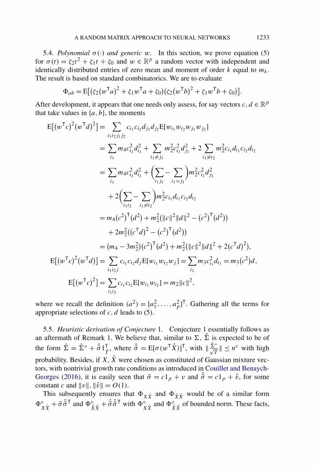
A RANDOM MATRIX APPROACH TO NEURAL NETWORKS 1233
5.4. Polynomial σ(·) and generic w. In this section, we prove equation (5)for σ(t) = ζ2t
2 + ζ1t + ζ0 and w ∈ Rp a random vector with independent and
identically distributed entries of zero mean and moment of order k equal to mk .The result is based on standard combinatorics. We are to evaluate
�ab = E[(
ζ2(wTa)2 + ζ1w
Ta + ζ0)(
ζ2(wTb)2 + ζ1w
Tb + ζ0)]
.
After development, it appears that one needs only assess, for say vectors c, d ∈ Rp
that take values in {a, b}, the moments
E[(
wTc)2(
wTd)2]= ∑
i1i2j1j2
ci1ci2dj1dj2E[wi1wi2wj1wj2]
= ∑i1
m4c2i1d2i1
+ ∑i1 =j1
m22c
2i1d2j1
+ 2∑i1 =i2
m22ci1di1ci2di2
= ∑i1
m4c2i1d2i1
+(∑
i1j1
− ∑i1=j1
)m2
2c2i1d2j1
+ 2(∑
i1i2
− ∑i1 =i2
)m2
2ci1di1ci2di2
= m4(c2)T(d2)+ m2
2(‖c‖2‖d‖2 − (c2)T(d2))
+ 2m22((
cTd)2 − (c2)T(d2))
= (m4 − 3m22)(
c2)T(d2)+ m22(‖c‖2‖d‖2 + 2
(cTd)2)
,
E[(
wTc)2(
wTd)]= ∑
i1i2j
ci1ci2dj E[wi1wi2wj ] =∑i1
m3c2i1di1 = m3
(c2)d,
E[(
wTc)2]= ∑
i1i2
ci1ci2E[wi1wi2] = m2‖c‖2,
where we recall the definition (a2) = [a21, . . . , a2
p]T. Gathering all the terms forappropriate selections of c, d leads to (5).
5.5. Heuristic derivation of Conjecture 1. Conjecture 1 essentially follows asan aftermath of Remark 1. We believe that, similar to �, � is expected to be of
the form � = �◦ + ˆσ1TT
, where ˆσ = E[σ(wTX)]T, with ‖ �◦√T‖ ≤ nε with high
probability. Besides, if X, X were chosen as constituted of Gaussian mixture vec-tors, with nontrivial growth rate conditions as introduced in Couillet and Benaych-Georges (2016), it is easily seen that σ = c1p + v and ˆσ = c1p + v, for someconstant c and ‖v‖,‖v‖ = O(1).
This subsequently ensures that �XX
and �XX
would be of a similar form
�◦XX
+ σ ˆσ T and �◦XX
+ ˆσ ˆσ T with �◦XX
and �◦XX
of bounded norm. These facts,
1234 C. LOUART, Z. LIAO AND R. COUILLET
that would require more advanced proof techniques, let envision the followingheuristic derivation for Conjecture 1.
Recall that our interest is on the test performance Etest defined as
Etest = 1
T
∥∥Y T − �Tβ∥∥2F ,
which may be rewritten as
Etest = 1
Ttr(Y Y T)− 2
T Ttr(YQ�T�Y T)+ 1
T 2Ttr(YQ�T��T�QY T)
(12)≡ Z1 − Z2 + Z3.
If � = �◦ + ˆσ1TT
follows the aforementioned claimed operator norm control, re-producing the steps of Corollary 3 leads to a similar concentration for Etest, whichwe shall then admit. We are therefore left to evaluating E[Z2] and E[Z3].
We start with the term E[Z2], which we expand as
E[Z2] = 2
T TE[tr(YQ�T�Y T)]= 2
T T
n∑i=1
[tr(YQσiσ
Ti Y T)]
= 2
T T
n∑i=1
E[tr(
YQ−iσi σTi Y T
1 + 1Tσ T
i Q−iσi
)]
= 2
T T
1
1 + δ
n∑i=1
E[tr(YQ−iσi σ
Ti Y T)]
+ 2
T T
1
1 + δ
n∑i=1
E[tr(YQ−iσi σ
Ti Y T)δ − 1
Tσ T
i Q−iσi
1 + 1Tσ T
i Q−iσi
]
= 2n
T T
1
1 + δtr(YE[Q−]�
XXY T)+ 2
T T
1
1 + δE[tr(YQ�TD�Y T)]
≡ Z21 + Z22
with D = diag({δ − 1Tσ T
i Q−iσi}), the operator norm of which is bounded by nε− 12
with high probability. Now, observe that, again with the assumption that � = �◦ +σ1T
Twith controlled �◦, Z22 may be decomposed as
2
T T
1
1 + δE[tr(YQ�TD�Y T)]= 2
T T
1
1 + δE[tr(YQ�TD�◦Y T)]
+ 2
T T
1
1 + δ1TTY TE[YQ�TDσ
].
In the display above, the first right-hand side term is now of order O(nε− 12 ). As
for the second right-hand side term, note that Dσ is a vector of independent and
A RANDOM MATRIX APPROACH TO NEURAL NETWORKS 1235
identically distributed zero mean and variance O(n−1) entries; while note formallyindependent of YQ�T, it is nonetheless expected that this independence “weak-ens” asymptotically (a behavior several times observed in linear random matrixmodels), so that one expects by central limit arguments that the second right-hand
side term be also of order O(nε− 12 ).
This would thus result in
E[Z2] = 2n
T T
1
1 + δtr(YE[Q−]�
XXY T)+ O
(nε− 1
2)
= 2n
T T
1
1 + δtr(YQ�
XXY T)+ O
(nε− 1
2)
= 2
Ttr(YQ
XXY T)+ O
(nε− 1
2),
where we used ‖E[Q−] − Q‖ ≤ Cnε− 12 and the definition
XX= n
T
�XX
1+δ.
We then move on to E[Z3] of equation (12), which can be developed as
E[Z3] = 1
T 2TE[tr(YQ�T��T�QY T)]
= 1
T 2T
n∑i,j=1
E[tr(YQσiσ
Ti σj σ
Tj QY T)]
= 1
T 2T
n∑i,j=1
E[tr(Y
Q−iσi σTi
1 + 1Tσ T
i Q−iσi
σj σTj Q−j
1 + 1Tσ T
j Q−jσj
Y T)]
= 1
T 2T
n∑i=1
∑j =i
E[tr(Y
Q−iσi σTi
1 + 1Tσ T
i Q−iσi
σj σTj Q−j
1 + 1Tσ T
j Q−jσj
Y T)]
+ 1
T 2T
n∑i=1
E[tr(Y
Q−iσi σTi σiσ
Ti Q−i
(1 + 1Tσ T
i Q−iσi)2Y T)]
≡ Z31 + Z32.
In the term Z32, reproducing the proof of Lemma 1 with the condition ‖X‖bounded, we obtain that
σTi σi
Tconcentrates around 1
Ttr�
XX, which allows us to
write
Z32 = 1
T 2T
n∑i=1
E[tr(Y
Q−iσi tr(�XX
)σ Ti Q−i
(1 + 1Tσ T
i Q−iσi)2Y T)]
+ 1
T 2T
n∑i=1
E[tr(Y
Q−iσi(σTi σi − tr�
T)σ T
i Q−i
(1 + 1Tσ T
i Q−iσi)2Y T)]
= 1
T 2
tr(�XX
)
T
n∑i=1
E[tr(Y
Q−iσiσTi Q−i
(1 + 1Tσ T
i Q−iσi)2Y T)]
1236 C. LOUART, Z. LIAO AND R. COUILLET
+ 1
T 2
n∑i=1
E[tr(YQσi
(σ T
i σi − tr�T
T
)σ T
i QY T)]
≡ Z321 + Z322
with D = diag({ 1Tσ T
i σi − 1T
tr�T T
}ni=1) and thus Z322 can be rewritten as
Z322 = 1
TE[tr(Y
Q�T
√T
D�Q√
TY T)]
= O(nε− 1
2)
while for Z321, following the same arguments as previously, we have
Z321 = 1
T 2
tr�XX
T
n∑i=1
E[tr(Y
Q−iσiσTi Q−i
(1 + 1Tσ T
i Q−iσi)2Y T)]
= 1
T 2
tr�XX
T
n∑i=1
1
(1 + δ)2 E[tr(YQ−iσiσ
Ti Q−iY
T)]
+ 1
T 2
tr�XX
T
n∑i=1
1
(1 + δ)2
× E[tr(YQσiσ
Ti QY T)((1 + δ)2 −
(1 + 1
Tσ T
i Q−iσi
)2)]
= 1
T 2
tr�XX
T
n∑i=1
1
(1 + δ)2 E[tr(YQ−i�XQ−iY
T)]
+ 1
T 2
tr�XX
T
n∑i=1
1
(1 + δ)2 E[tr(YQ�TD�QY T)]
= n
T 2 E[tr(YQ−�XQ−Y T)] tr(�
XX)
T (1 + δ)2+ O
(nε− 1
2),
where D = diag({(1 + δ)2 − (1 + 1Tσ T
i Q−iσi)2}ni=1).
Since E[Q−AQ−] = E[QAQ]+O‖·‖(nε− 12 ), we are free to plug in the asymp-
totic equivalent of E[QAQ] derived in Section 5.2.3, and we deduce
Z32 = n
T 2 E[trY(Q�XQ + Q XQ · 1
ntr( XQ�XQ)
1 − 1n
tr( 2XQ2)
)Y T] tr(�
XX)
T (1 + δ)2
=1n
tr(Y Q XQY T)
1 − 1n
tr( 2XQ2)
1
Ttr(
XX) + O
(nε− 1
2).
The term Z31 of the double sum over i and j (j = i) needs more efforts. Tohandle this term, we need to remove the dependence of both σi and σj in Q in

A RANDOM MATRIX APPROACH TO NEURAL NETWORKS 1237
sequence. We start with j as follows:
Z31 = 1
T 2T
n∑i=1
∑j =i
E[tr(YQσiσ
Ti
σj σTj Q−j
1 + 1Tσ T
j Q−j σj
Y T)]
= 1
T 2T
n∑i=1
∑j =i
E[tr(YQ−j σi σ
Ti
σj σTj Q−j
1 + 1Tσ T
j Q−jσj
Y T)]
− 1
T 3T
n∑i=1
∑j =i
E[tr(Y
Q−j σjσTj Q−jσi σ
Ti
1 + 1Tσ T
j Q−jσj
σj σTj Q−j
1 + 1Tσ T
j Q−jσj
Y T)]
≡ Z311 − Z312,
where in the previous to last inequality we used the relation
Q = Q−j − Q−j σjσTj Q−j
1 + 1Tσ T
j Q−j σj
.
For Z311, we replace 1 + 1Tσ T
j Q−j σj by 1 + δ and take expectation over wj :
Z311 = 1
T 2T
n∑i=1
∑j =i
E[tr(YQ−j σi σ
Ti
σj σTj Q−j
1 + 1Tσ T
j Q−j σj
Y T)]
= 1
T 2T
n∑j=1
E[tr(Y
Q−j�T−j �−j σj σ
Tj Q−j
1 + 1Tσ T
j Q−j σj
Y T)]
= 1
T 2T
1
1 + δ
n∑j=1
E[tr(YQ−j�
T−j �−j σj σTj Q−jY
T)]
+ 1
T 2T
1
1 + δ
n∑j=1
E[tr(Y
Q−j�T−j �−j σj σ
Tj Q−j (δ − 1
Tσ T
j Q−jσj )
1 + 1Tσ T
j Q−j σj
Y T)]
≡ Z3111 + Z3112.
The idea to handle Z3112 is to retrieve forms of the type∑n
j=1 dj σjσTj = �TD�
for some D satisfying ‖D‖ ≤ nε− 12 with high probability. To this end, we use
Q−j
�T−j �−j
T= Q−j
�T�
T− Q−j
σj σTj
T
= Q�T�
T+ Qσjσ
Tj Q
1 − 1Tσ T
j Qσj
�T�
T− Q−j
σj σTj
T

1238 C. LOUART, Z. LIAO AND R. COUILLET
and thus Z3112 can be expanded as the sum of three terms that shall be studied inorder:
Z3112 = 1
T 2T
1
1 + δ
n∑j=1
E[tr(Y
Q−j�T−j �−j σj σ
Tj Q−j (δ − 1
Tσ T
j Q−jσj )
1 + 1Tσ T
j Q−j σj
Y T)]
= 1
T T
1
1 + δE[tr(YQ
�T�
T�TD�QY T
)]
+ 1
T T
1
1 + δ
n∑j=1
E[tr(Y
QσjσTj Q�T�σj (δ − 1
Tσ T
j Q−j σj )σTj Q
T (1 − 1Tσ T
j Qσj )Y T)]
− 1
T 2T
1
1 + δ
n∑j=1
E[tr(YQσj σ
Tj σj σ
Tj Q
(δ − 1
Tσ T
j Q−jσj
)
×(
1 + 1
Tσ T
j Q−j σj
)Y T)]
≡ Z31121 + Z31122 − Z31123,
where D = diag({δ − 1Tσ T
j Q−j σj }ni=1). First, Z31121 is of order O(nε− 12 ) since
Q�T�T
is of bounded operator norm. Subsequently, Z31122 can be rewritten as
Z31122 = 1
T
1
1 + δE[tr(YQ
�TD�
TQY T
)]= O
(nε− 1
2)
with here
D = diag{((
δ − 1
Tσ T
j Q−j σj
)(1
Ttr(Q−j
�T−j �−j
T�
XX
)
+ 1
Ttr(Q−j�)
1
Ttr�
XX
))/((
1 − 1
Tσ T
j Qσj
)(1 + 1
Tσ T
j Q−jσj
))}n
i=1.
The same arguments apply for Z31123 but for
D = diag{ tr�
XX
T
(δ − 1
Tσ T
j Q−j σj
)(1 + 1
Tσ T
j Q−j σj
)}n
i=1,
which completes to show that |Z3112| ≤ Cnε− 12 and thus
Z311 = Z3111 + O(nε− 1
2)
= 1
T 2T
1
1 + δ
n∑j=1
E[tr(YQ−j�
T−j �−j σj σTj Q−jY
T)]+ O(nε− 1
2).
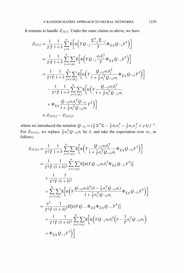
A RANDOM MATRIX APPROACH TO NEURAL NETWORKS 1239
It remains to handle Z3111. Under the same claims as above, we have
Z3111 = 1
T T
1
1 + δ
n∑j=1
E[tr(YQ−j
�T−j �−j
T�
XXQ−jY
T)]
= 1
T T
1
1 + δ
n∑j=1
∑i =j
E[tr(YQ−j
σi σTi
T�
XXQ−jY
T)]
= 1
T 2T
1
1 + δ
n∑j=1
∑i =j
E[tr(Y
Q−ij σi σTi
1 + 1Tσ T
i Q−ij σi
�XX
Q−ij YT)]
− 1
T 3T
1
1 + δ
n∑j=1
∑i =j
E[tr(Y
Q−ij σi σTi
1 + 1Tσ T
i Q−ij σi
× �XX
Q−ij σiσTi Q−ij
1 + 1Tσ T
i Q−ij σi
Y T)]
≡ Z31111 − Z31112,
where we introduced the notation Q−ij = ( 1T�T� − 1
Tσiσ
Ti − 1
Tσjσ
Tj + γ IT )−1.
For Z31111, we replace 1Tσ T
i Q−ij σi by δ, and take the expectation over wi , asfollows:
Z31111 = 1
T 2T
1
1 + δ
n∑j=1
∑i =j
E[tr(Y
Q−ij σi σTi
1 + 1Tσ T
i Q−ij σi
�XX
Q−ij YT)]
= 1
T 2T
1
(1 + δ)2
n∑j=1
∑i =j
E[tr(YQ−ij σi σ
Ti �
XXQ−ij Y
T)]
+ 1
T 2T
1
(1 + δ)2
×n∑
j=1
∑i =j
E[tr(Y
Q−ij σi σTi (δ − 1
Tσ T
i Q−ij σi)
1 + 1Tσ T
i Q−ij σi
�XX
Q−ij YT)]
= n2
T 2T
1
(1 + δ)2 E[tr(YQ−−�
XX�
XXQ−−Y T)]
+ 1
T 2T
1
(1 + δ)2
n∑j=1
∑i =j
E[tr(YQ−j σi σ
Ti
(δ − 1
Tσ T
i Q−ij σi
)
× �XX
Q−jYT)]
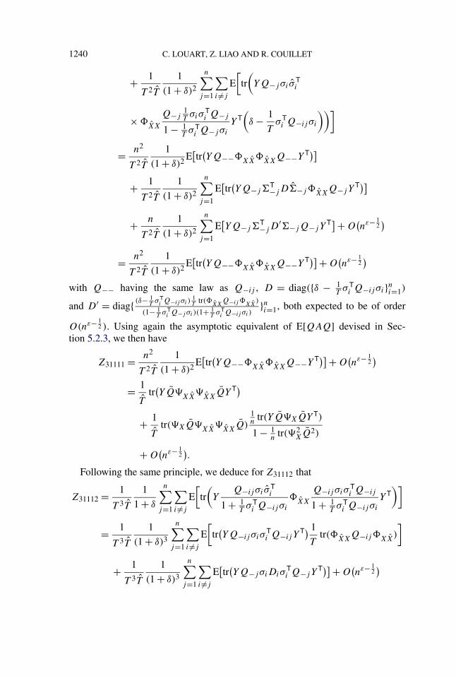
1240 C. LOUART, Z. LIAO AND R. COUILLET
+ 1
T 2T
1
(1 + δ)2
n∑j=1
∑i =j
E[tr(YQ−j σi σ
Ti
× �XX
Q−j1Tσiσ
Ti Q−j
1 − 1Tσ T
i Q−jσi
Y T(δ − 1
Tσ T
i Q−ij σi
))]
= n2
T 2T
1
(1 + δ)2 E[tr(YQ−−�
XX�
XXQ−−Y T)]
+ 1
T 2T
1
(1 + δ)2
n∑j=1
E[tr(YQ−j�
T−jD�−j�XXQ−jY
T)]
+ n
T 2T
1
(1 + δ)2
n∑j=1
E[YQ−j�
T−jD′�−jQ−jY
T]+ O(nε− 1
2)
= n2
T 2T
1
(1 + δ)2 E[tr(YQ−−�
XX�
XXQ−−Y T)]+ O
(nε− 1
2)
with Q−− having the same law as Q−ij , D = diag({δ − 1Tσ T
i Q−ij σi}ni=1)
and D′ = diag{ (δ− 1T
σTi Q−ij σi )
1T
tr(�XX
Q−ij �XX
)
(1− 1T
σTi Q−j σi )(1+ 1
TσT
i Q−ij σi )}ni=1, both expected to be of order
O(nε− 12 ). Using again the asymptotic equivalent of E[QAQ] devised in Sec-
tion 5.2.3, we then have
Z31111 = n2
T 2T
1
(1 + δ)2 E[tr(YQ−−�
XX�
XXQ−−Y T)]+ O
(nε− 1
2)
= 1
Ttr(YQ
XX
XXQY T)
+ 1
Ttr( XQ
XX
XXQ)
1n
tr(Y Q XQY T)
1 − 1n
tr( 2XQ2)
+ O(nε− 1
2).
Following the same principle, we deduce for Z31112 that
Z31112 = 1
T 3T
1
1 + δ
n∑j=1
∑i =j
E[tr(Y
Q−ij σi σTi
1 + 1Tσ T
i Q−ij σi
�XX
Q−ij σiσTi Q−ij
1 + 1Tσ T
i Q−ij σi
Y T)]
= 1
T 3T
1
(1 + δ)3
n∑j=1
∑i =j
E[tr(YQ−ij σiσ
Ti Q−ij Y
T) 1
Ttr(�
XXQ−ij�XX
)
]
+ 1
T 3T
1
(1 + δ)3
n∑j=1
∑i =j
E[tr(YQ−j σiDiσ
Ti Q−jY
T)]+ O(nε− 1
2)

A RANDOM MATRIX APPROACH TO NEURAL NETWORKS 1241
= n2
T 3T
1
1 + δE[tr(YQ−−�XQ−−Y T) 1
Ttr(�
XXQ−−�
XX)
]
+ O(nε− 1
2)
= 1
Ttr(
XXQ
XX)
1n
tr(Y Q XQY T)
1 − 1n
tr( 2XQ2)
+ O(nε− 1
2)
with Di = 1T
tr(�XX
Q−ij�XX)[(1 + δ)2 − (1 + 1
Tσ T
i Q−ij σi)2], also believed to
be of order O(nε− 12 ). Recalling the fact that Z311 = Z3111 +O(nε− 1
2 ), we can thusconclude for Z311 that
Z311 = 1
Ttr(YQ
XX
XXQY T)
+ 1
Ttr( XQ
XX
XXQ)
1n
tr(Y Q XQY T)
1 − 1n
tr( 2XQ2)
− 1
Ttr(
XXQ
XX)
1n
tr(Y Q XQY T)
1 − 1n
tr( 2XQ2)
+ O(nε− 1
2).
As for Z312, we have
Z312 = 1
T 3T
n∑i=1
∑j =i
E[tr(Y
Q−j σjσTj Q−jσi σ
Ti
1 + 1Tσ T
j Q−jσj
σj σTj Q−j
1 + 1Tσ T
j Q−jσj
Y T)]
= 1
T 3T
n∑j=1
E[tr(Y
Q−j σjσTj Q−j�
T−j �−j
1 + 1Tσ T
j Q−j σj
σj σTj Q−j
1 + 1Tσ T
j Q−j σj
Y T)]
.
Since Q−j1T�T−j �−j is expected to be of bounded norm, using the concentration
inequality of the quadratic form 1Tσ T
j Q−j�T−j �−j
Tσj , we infer
Z312 = 1
T T
n∑j=1
E[tr(Y
Q−j σjσTj Q−jY
T
(1 + 1Tσ T
j Q−j σj )2
)
×(
1
T 2 tr(Q−j�
T−j �−j�XX
)+ O(nε− 1
2))]
= 1
T T
n∑j=1
E[tr(Y
Q−j σjσTj Q−jY
T
(1 + 1Tσ T
j Q−j σj )2
)(1
T 2 tr(Q−j�
T−j �−j�XX
))]
+ O(nε− 1
2).

1242 C. LOUART, Z. LIAO AND R. COUILLET
We again replace 1Tσ T
j Q−jσj by δ and take expectation over wj to obtain
Z312 = 1
T T
1
(1 + δ)2
n∑j=1
E[tr(YQ−j σjσ
Tj Q−jY
T) 1
T 2 tr(Q−j�
T−j �−j�XX
)]
+ 1
T T
1
(1 + δ)2
×n∑
j=1
E[ tr(YQ−j σjDjσ
Tj Q−jY
T)
(1 + 1Tσ T
j Q−j σj )2
1
T 2 tr(Q−j�
T−j �−j�XX
)]
+ O(nε− 1
2)
= n
T T
1
(1 + δ)2 E[tr(YQ−�XQ−Y T) 1
T 2 tr(Q−�T−�−�
XX
)]
+ 1
T T
1
(1 + δ)2 E[tr(YQ�TD�QY T) 1
T 2 tr(Q−�T−�−�
XX
)]+ O(nε− 1
2)
with Dj = (1 + δ)2 − (1 + 1Tσ T
j Q−jσj )2 = O(nε− 1
2 ), which eventually brings thesecond term to vanish, and we thus get
Z312 = n
T T
1
(1 + δ)2 E[tr(YQ−�XQ−Y T) 1
T 2 tr(Q−�T−�−�
XX
)]+ O(nε− 1
2).
For the term 1T 2 tr(Q−�T−�−�
XX) we apply again the concentration inequality
to get
1
T 2 tr(Q−�T−�−�
XX
)
= 1
T 2
∑i =j
tr(Q−j σi σ
Ti �
XX
)
= 1
T 2
∑i =j
tr(
Q−ij σi σTi
1 + 1Tσ T
i Q−ij σi
�XX
)
= 1
T 2
1
1 + δ
∑i =j
tr(Q−ij σi σ
Ti �
XX
)
+ 1
T 2
1
1 + δ
∑i =j
tr(
Q−ij σi σTi (δ − 1
Tσ T
i Q−ij σi)
1 + 1Tσ T
i Q−ij σi
�XX
)
= n − 1
T 2
1
1 + δtr(�
XXE[Q−−]�
XX
)
+ 1
T 2
1
1 + δtr(Q−j�
T−jD�−j�XX
)+ O(nε− 1
2)
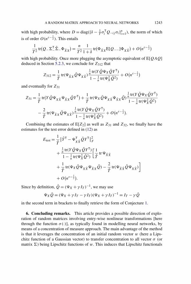
A RANDOM MATRIX APPROACH TO NEURAL NETWORKS 1243
with high probability, where D = diag({δ − 1Tσ T
i Q−ij σi}ni=1), the norm of which
is of order O(nε− 12 ). This entails
1
T 2 tr(Q−�T−�−�
XX
)= n
T 2
1
1 + δtr(�
XXE[Q−−]�
XX
)+ O(nε− 1
2)
with high probability. Once more plugging the asymptotic equivalent of E[QAQ]deduced in Section 5.2.3, we conclude for Z312 that
Z312 = 1
Ttr(
XXQ
XX)
1n
tr(Y Q XQY T)
1 − 1n
tr( 2XQ2)
+ O(nε− 1
2)
and eventually for Z31
Z31 = 1
Ttr(YQ
XX
XXQY T)+ 1
Ttr( XQ
XX
XXQ)
1n
tr(Y Q XQY T)
1 − 1n
tr( 2XQ2)
− 2
Ttr(
XXQ
XX)
1n
tr(Y Q XQY T)
1 − 1n
tr( 2XQ2)
+ O(nε− 1
2).
Combining the estimates of E[Z2] as well as Z31 and Z32, we finally have theestimates for the test error defined in (12) as
Etest = 1
T
∥∥Y T − TXX
QY T∥∥2F
+1n
tr(Y Q XQY T)
1 − 1n
tr( 2XQ2)
[1
Ttr
XX
+ 1
Ttr( XQ
XX
XXQ) − 2
Ttr(
XXQ
XX)
]
+ O(nε− 1
2).
Since by definition, Q = ( X + γ IT )−1, we may use
XQ = ( X + γ IT − γ IT )( X + γ IT )−1 = IT − γ Q
in the second term in brackets to finally retrieve the form of Conjecture 1.
6. Concluding remarks. This article provides a possible direction of explo-ration of random matrices involving entry-wise nonlinear transformations [herethrough the function σ(·)], as typically found in modelling neural networks, bymeans of a concentration of measure approach. The main advantage of the methodis that it leverages the concentration of an initial random vector w (here a Lips-chitz function of a Gaussian vector) to transfer concentration to all vector σ (ormatrix �) being Lipschitz functions of w. This induces that Lipschitz functionals
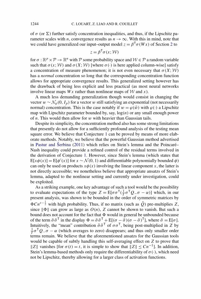
1244 C. LOUART, Z. LIAO AND R. COUILLET
of σ (or �) further satisfy concentration inequalities, and thus, if the Lipschitz pa-rameter scales with n, convergence results as n → ∞. With this in mind, note thatwe could have generalized our input–output model z = βTσ(Wx) of Section 2 to
z = βTσ(x;W)
for σ : Rp ×P →Rn with P some probability space and W ∈ P a random variable
such that σ(x;W) and σ(X;W) [where σ(·) is here applied column-wise] satisfya concentration of measure phenomenon; it is not even necessary that σ(X;W)
has a normal concentration so long that the corresponding concentration functionallows for appropriate convergence results. This generalized setting however hasthe drawback of being less explicit and less practical (as most neural networksinvolve linear maps Wx rather than nonlinear maps of W and x).
A much less demanding generalization though would consist in changing thevector w ∼ Nϕ(0, Ip) for a vector w still satisfying an exponential (not necessarilynormal) concentration. This is the case notably if w = ϕ(w) with ϕ(·) a Lipschitzmap with Lipschitz parameter bounded by, say, log(n) or any small enough powerof n. This would then allow for w with heavier than Gaussian tails.
Despite its simplicity, the concentration method also has some strong limitationsthat presently do not allow for a sufficiently profound analysis of the testing meansquare error. We believe that Conjecture 1 can be proved by means of more elab-orate methods. Notably, we believe that the powerful Gaussian method advertisedin Pastur and Serbina (2011) which relies on Stein’s lemma and the Poincaré–Nash inequality could provide a refined control of the residual terms involved inthe derivation of Conjecture 1. However, since Stein’s lemma (which states thatE[xφ(x)] = E[φ′(x)] for x ∼ N (0,1) and differentiable polynomially bounded φ)can only be used on products xφ(x) involving the linear component x, the latter isnot directly accessible; we nonetheless believe that appropriate ansatzs of Stein’slemma, adapted to the nonlinear setting and currently under investigation, couldbe exploited.
As a striking example, one key advantage of such a tool would be the possibilityto evaluate expectations of the type Z = E[σσ T( 1
Tσ TQ−σ − α)] which, in our
present analysis, was shown to be bounded in the order of symmetric matrices by
�Cnε− 12 with high probability. Thus, if no matrix (such as Q) pre-multiplies Z,
since ‖�‖ can grow as large as O(n), Z cannot be shown to vanish. But such abound does not account for the fact that � would in general be unbounded becauseof the term σ σ T in the display � = σ σ T + E[(σ − σ )(σ − σ )T], where σ = E[σ ].Intuitively, the “mean” contribution σ σ T of σσ T, being post-multiplied in Z by1Tσ TQ−σ − α (which averages to zero) disappears; and thus only smaller order
terms remain. We believe that the aforementioned ansatzs for the Gaussian toolswould be capable of subtly handling this self-averaging effect on Z to prove that‖Z‖ vanishes [for σ(t) = t , it is simple to show that ‖Z‖ ≤ Cn−1]. In addition,Stein’s lemma-based methods only require the differentiability of σ(·), which neednot be Lipschitz, thereby allowing for a larger class of activation functions.
A RANDOM MATRIX APPROACH TO NEURAL NETWORKS 1245
As suggested in the simulations of Figure 2, our results also seem to extend tononcontinuous functions σ(·). To date, we cannot envision a method allowing totackle this setting.
In terms of neural network applications, the present article is merely a first steptowards a better understanding of the “hardening” effect occurring in large dimen-sional networks with numerous samples and large data points (i.e., simultaneouslylarge n,p,T ), which we exemplified here through the convergence of mean-squareerrors. The mere fact that some standard performance measure of these randomnetworks would “freeze” as n,p,T grow at the predicted regime and that the per-formance would heavily depend on the distribution of the random entries is alreadyin itself an interesting result to neural network understanding and dimensioning.However, more interesting questions remain open. Since neural networks are to-day dedicated to classification rather than regression, a first question is the studyof the asymptotic statistics of the output z = βTσ(Wx) itself; we believe that z
satisfies a central limit theorem with mean and covariance allowing for assessingthe asymptotic misclassification rate.
A further extension of the present work would be to go beyond the single-layernetwork and include multiple layers (finitely many or possibly a number scalingwith n) in the network design. The interest here would be on the key question ofthe best distribution of the number of neurons across the successive layers.
It is also classical in neural networks to introduce different (possibly random)biases at the neuron level, thereby turning σ(t) into σ(t +b) for a random variableb different for each neuron. This has the effect of mitigating the negative impactof the mean E[σ(wT
i xj )], which is independent of the neuron index i.Finally, neural networks, despite their having been recently shown to operate al-
most equally well when taken random in some very specific scenarios, are usuallyonly initiated as random networks before being subsequently trained through back-propagation of the error on the training dataset (i.e., essentially through convexgradient descent). We believe that our framework can allow for the understandingof at least finitely many steps of gradient descent, which may then provide furtherinsights into the overall performance of deep learning networks.
APPENDIX: INTERMEDIARY LEMMAS
This section recalls some elementary algebraic relations and identities usedthroughout the proof section.
LEMMA 5 (Resolvent identity). For invertible matrices A,B , A−1 − B−1 =A−1(B − A)B−1.
LEMMA 6 (A rank-1 perturbation identity). For A Hermitian, v a vector andt ∈ R, if A and A + tvvT are invertible, then
(A + tvvT)−1
v = A−1v
1 + tvTA−1v.

1246 C. LOUART, Z. LIAO AND R. COUILLET
LEMMA 7 (Operator norm control). For nonnegative definite A and z ∈ C \R
+, ∥∥(A − zIT )−1∥∥≤ dist(z,R+)−1
,∥∥A(A − zIT )−1∥∥≤ 1,
where dist(x,A) is the Hausdorff distance of a point to a set. In particular, forγ > 0, ‖(A + γ IT )−1‖ ≤ γ −1 and ‖A(A + γ IT )−1‖ ≤ 1.
REFERENCES
AKHIEZER, N. I. and GLAZMAN, I. M. (1993). Theory of Linear Operators in Hilbert Space. Dover,New York. MR1255973
BAI, Z. D. and SILVERSTEIN, J. W. (1998). No eigenvalues outside the support of the limitingspectral distribution of large-dimensional sample covariance matrices. Ann. Probab. 26 316–345.MR1617051
BAI, Z. D. and SILVERSTEIN, J. W. (2007). On the signal-to-interference-ratio of CDMA systemsin wireless communications. Ann. Appl. Probab. 17 81–101. MR2292581
BAI, Z. and SILVERSTEIN, J. W. (2010). Spectral Analysis of Large Dimensional Random Matrices,2nd ed. Springer, New York. MR2567175
BENAYCH-GEORGES, F. and NADAKUDITI, R. R. (2012). The singular values and vectors of lowrank perturbations of large rectangular random matrices. J. Multivariate Anal. 111 120–135.
CAMBRIA, E., GASTALDO, P., BISIO, F. and ZUNINO, R. (2015). An ELM-based model for affec-tive analogical reasoning. Neurocomputing 149 443–455.
CHOROMANSKA, A., HENAFF, M., MATHIEU, M., AROUS, G. B. and LECUN, Y. (2015). Theloss surfaces of multilayer networks. In AISTATS.
COUILLET, R. and BENAYCH-GEORGES, F. (2016). Kernel spectral clustering of large dimensionaldata. Electron. J. Stat. 10 1393–1454.
COUILLET, R., HOYDIS, J. and DEBBAH, M. (2012). Random beamforming over quasi-static andfading channels: A deterministic equivalent approach. IEEE Trans. Inform. Theory 58 6392–6425.MR2982669
COUILLET, R. and KAMMOUN, A. (2016). Random matrix improved subspace clustering. In 2016Asilomar Conference on Signals, Systems, and Computers.
COUILLET, R., PASCAL, F. and SILVERSTEIN, J. W. (2015). The random matrix regime ofMaronna’s M-estimator with elliptically distributed samples. J. Multivariate Anal. 139 56–78.
EL KAROUI, N. (2009). Concentration of measure and spectra of random matrices: Applicationsto correlation matrices, elliptical distributions and beyond. Ann. Appl. Probab. 19 2362–2405.MR2588248
EL KAROUI, N. (2010). The spectrum of kernel random matrices. Ann. Statist. 38 1–50. MR2589315EL KAROUI, N. (2013). Asymptotic behavior of unregularized and ridge-regularized
high-dimensional robust regression estimators: Rigorous results. Preprint. Available atarXiv:1311.2445.
GIRYES, R., SAPIRO, G. and BRONSTEIN, A. M. (2016). Deep neural networks with random Gaus-sian weights: A universal classification strategy? IEEE Trans. Signal Process. 64 3444–3457.MR3515693
HORNIK, K., STINCHCOMBE, M. and WHITE, H. (1989). Multilayer feedforward networks areuniversal approximators. Neural Networks 2 359–366.
HUANG, G.-B., ZHU, Q.-Y. and SIEW, C.-K. (2006). Extreme learning machine: Theory and ap-plications. Neurocomputing 70 489–501.
A RANDOM MATRIX APPROACH TO NEURAL NETWORKS 1247
HUANG, G.-B., ZHOU, H., DING, X. and ZHANG, R. (2012). Extreme learning machine for re-gression and multiclass classification. Systems, Man, and Cybernetics, Part B: Cybernetics, IEEETransactions on 42 513–529.
JAEGER, H. and HAAS, H. (2004). Harnessing nonlinearity: Predicting chaotic systems and savingenergy in wireless communication. Science 304 78–80.
KAMMOUN, A., KHAROUF, M., HACHEM, W. and NAJIM, J. (2009). A central limit theorem forthe sinr at the lmmse estimator output for large-dimensional signals. IEEE Transactions on Infor-mation Theory 55 5048–5063.
KRIZHEVSKY, A., SUTSKEVER, I. and HINTON, G. E. (2012). Imagenet classification with deepconvolutional neural networks. In Advances in Neural Information Processing Systems 1097–1105.
LECUN, Y., CORTES, C. and BURGES, C. (1998). The MNIST database of handwritten digits.LEDOUX, M. (2005). The Concentration of Measure Phenomenon 89. Amer. Math. Soc., Providence,
RI. MR1849347LIAO, Z. and COUILLET, R. (2017). A large dimensional analysis of least squares support vector
machines. J. Mach. Learn. Res. To appear. Available at arXiv:1701.02967.LOUBATON, P. and VALLET, P. (2010). Almost sure localization of the eigenvalues in a Gaussian
information plus noise model. Application to the spiked models. Electron. J. Probab. 16 1934–1959.
MAI, X. and COUILLET, R. (2017). The counterintuitive mechanism of graph-based semi-supervised learning in the big data regime. In IEEE International Conference on Acoustics,Speech and Signal Processing (ICASSP’17).
MARCENKO, V. A. and PASTUR, L. A. (1967). Distribution of eigenvalues for some sets of randommatrices. Math. USSR, Sb. 1 457–483.
PASTUR, L. and SERBINA, M. (2011). Eigenvalue Distribution of Large Random Matrices. Amer.Math. Soc., Providence, RI. MR2808038
RAHIMI, A. and RECHT, B. (2007). Random features for large-scale kernel machines. In Advancesin Neural Information Processing Systems 1177–1184.
ROSENBLATT, F. (1958). The perceptron: A probabilistic model for information storage and organi-zation in the brain. Psychol. Rev. 65 386–408.
RUDELSON, M., VERSHYNIN, R. et al. (2013). Hanson–Wright inequality and sub-Gaussian con-centration. Electron. Commun. Probab. 18 1–9.
SAXE, A., KOH, P. W., CHEN, Z., BHAND, M., SURESH, B. and NG, A. Y. (2011). On randomweights and unsupervised feature learning. In Proceedings of the 28th International Conferenceon Machine Learning (ICML-11) 1089–1096.
SCHMIDHUBER, J. (2015). Deep learning in neural networks: An overview. Neural Netw. 61 85–117.SILVERSTEIN, J. W. and BAI, Z. D. (1995). On the empirical distribution of eigenvalues of a class
of large dimensional random matrices. J. Multivariate Anal. 54 175–192.SILVERSTEIN, J. W. and CHOI, S. (1995). Analysis of the limiting spectral distribution of large
dimensional random matrices. J. Multivariate Anal. 54 295–309.TAO, T. (2012). Topics in Random Matrix Theory 132. Amer. Math. Soc., Providence, RI.TITCHMARSH, E. C. (1939). The Theory of Functions. Oxford Univ. Press, New York.VERSHYNIN, R. (2012). Introduction to the non-asymptotic analysis of random matrices. In Com-
pressed Sensing, 210–268, Cambridge Univ. Press, Cambridge.WILLIAMS, C. K. I. (1998). Computation with infinite neural networks. Neural Comput. 10 1203–
1216.YATES, R. D. (1995). A framework for uplink power control in cellular radio systems. IEEE Journal
on Selected Areas in Communications 13 1341–1347.ZHANG, T., CHENG, X. and SINGER, A. (2014). Marchenko–Pastur Law for Tyler’s and Maronna’s
M-estimators. Available at http://arxiv.org/abs/1401.3424.

1248 C. LOUART, Z. LIAO AND R. COUILLET
LABORATOIRE DES SIGNAUX ET SYSTÈMES
CENTRALESUPÉLEC
UNIVERSITY OF PARIS-SACLAY
3, RUE JOLIOT-CURIE
91192 GIF SUR YVETTE
FRANCE
E-MAIL: [email protected]@[email protected]
Related Documents


