A queueing system with discrete autoregressive arrivals

Performance Evaluation 64 (2007) 148–161www.elsevier.com/locate/peva

A queueing system with discrete autoregressive arrivalsI

Bara Kima,∗, Yong Changb, Yeong Cheol Kimc, Bong Dae Choia

a Department of Mathematics and Telecommunication Mathematics Research Center, Korea University, 1, Anam-dong, Sungbuk-ku, Seoul,136-701, Republic of Korea

b Telecommunication Systems Division, Information and Communication Business, Samsung Electronics Co., Ltd, Suwon-si, Gyeonggi-do,442-742, Republic of Korea

c Department of Mathematics, Mokpo National University, Muan-gun, Chonnam, 534-729, Republic of Korea

Received 29 April 2003; received in revised form 3 March 2006Available online 7 July 2006

Abstract

We consider a discrete time single server queue with discrete autoregressive process of order 1 (DAR(1)) input. By extractinga Markov process from the queue size process and applying the BASTA property, we derive simple recursive formulae for thestationary distributions of the queue size and the waiting time. These formulae are simple, numerically stable and transform-free. A stochastic decomposition property is given for the stationary waiting time, and relations between the distributions of thestationary queue size and the stationary waiting time are discussed. Numerical examples are given for stationary distributions ofthe queue size and the waiting time for various DAR(1) inputs.c© 2006 Elsevier B.V. All rights reserved.

Keywords: DAR(1); Discrete time queue; Queue size; Waiting time; Recursive formula; Stochastic decomposition

1. Introduction

The discrete autoregressive process of order 1 (abbreviated by DAR(1)) is described by a small number ofparameters and it is known that DAR(1) is a good candidate to model video teleconference traffic in telecommunicationnetworks [5,6]. The parameters for the stationary distribution and the correlation function in the DAR(1) model canbe determined from measured real traffic. Further, many queueing systems with DAR(1) inputs are mathematicallytractable.

Many analyses for DAR(1) queueing models are found in recent works. For a discrete time single server queuewith DAR(1) input, Hwang and Sohraby [5] derived the probability generating function of the stationary queue size,Hwang et al. [6] derived the probability generating function of the stationary waiting time, and Kim and Sohraby [7]found a necessary and sufficient condition for the queue size and waiting time to have asymptotically geometric taildistributions. Kim and Sohraby [8] proved that if the stationary distribution of the DAR(1) has a regularly varying tail,

I This work was supported by grant No. R01-2001-00007 from the Korea Science & Engineering Foundation.∗ Corresponding author.

E-mail addresses: [email protected] (B. Kim), [email protected] (Y. Chang), [email protected] (Y.C. Kim),[email protected] (B.D. Choi).

0166-5316/$ - see front matter c© 2006 Elsevier B.V. All rights reserved.doi:10.1016/j.peva.2006.05.008

http://www.elsevier.com/locate/peva

mailto:[email protected]




http://dx.doi.org/10.1016/j.peva.2006.05.008

B. Kim et al. / Performance Evaluation 64 (2007) 148–161 149

then the queue size and the waiting time also have regularly varying tails. For a discrete time multiserver queue withDAR(1) input, Choi et al. [3] obtained the stationary distributions of the queue size and the waiting time by using thematrix analytic method.

In this paper, we consider a discrete time single server queue with DAR(1) input. By using an embedded Markovchain and the BASTA (Bernoulli arrivals see time averages) property, we derive simple recursive formulae (seeTheorem 1, Corollaries 1 and 2) for the stationary distributions of the queue size and the waiting time. The meritsof the formulae in Theorem 1, Corollaries 1 and 2 are as follows: The formulae are simple, numerically stable andtransform-free. For calculation of the stationary distributions of the queue size and the waiting time, the results inthis paper are much more useful than those in [5,6], where probability generating functions of the queue size andthe waiting time are given. We also derive a stochastic decomposition property that the stationary waiting time canbe expressed as an independent sum of the stationary number of packets and a nonnegative integer-valued randomvariable. Then we discuss relations between the distributions of the stationary queue size and the stationary waitingtime (see Corollary 2 and subsequent remarks). Numerical examples are given for the stationary distributions ofthe queue size and the waiting time for various DAR(1) inputs. Numerical examples reflects the properties provenin [7,8]:

• The stationary distributions of the queue size and the waiting time in the queueing system with DAR(1) input areasymptotically geometric if and only if the stationary distribution of the DAR(1) has finite support;• The queue size and the waiting time have regularly varying tails if the stationary distribution of the DAR(1) has a

regularly varying tail.

The contributions in this paper are different from those in other works as follows: While we express the distributionsof the stationary queue size and the stationary waiting time in a transform-free form, Hwang et al. [5,6] expressedthe distributions in terms of the probability generating functions. Kim and Sohraby [7,8] investigated asymptoticproperties of the distributions of the stationary queue size and the stationary waiting time by using the probabilitygenerating functions. Choi et al. [3] anayzed the multiserver queue by using the matrix analytic method, where theirresults heavily rely on matrix manipulation even for the special case of the single server queue.

2. The DAR(1)/D/1 queue

Let B(t), t = 0, 1, 2, . . . , be independent and identically distributed (i.i.d.) random variables. We assume that B(t)takes nonnegative integers and denote bk = P{B(t) = k}, k = 0, 1, 2, . . .. The process {Y (t) : t = 0, 1, 2, . . .} definedby the following recursion is a DAR(1):

Y (0) = B(0);

Y (t) = (1− α(t))Y (t − 1)+ α(t)B(t), t = 1, 2, 3, . . . ,

where α(t), t = 1, 2, 3, . . . , are i.i.d. Bernoulli random variables with P{α(t) = 0} = β (0 ≤ β < 1) andP{α(t) = 1} = 1 − β, and {α(t) : t = 1, 2, 3, . . .} is assumed to be independent of {B(t) : t = 0, 1, 2, . . .}.The following are basic properties of DAR(1) (see, for example, [6]).

• {Y (t)} is stationary.• The probability distribution of Y (t) is the same as the distribution of B(t), i.e.,

P{Y (t) = k} = bk, k = 0, 1, 2, . . . .

• The autocorrelation function r(t) for {Y (t)} is given by

r(t) ≡Cov(Y (0), Y (t))

Var(Y (0))= β t , t = 0, 1, 2, . . . . (1)

Now we consider the DAR(1)/D/1 queue, where the time is divided into slots of equal size and one slot is neededto serve a packet. We assume that packet arrivals occur at the beginning of slots and departures occur at the end ofslots. Let Y (t), t = 0, 1, 2. . . . , represent the number of packets that arrive at the beginning of the t th slot. The orderof services are assumed to be based on the first-come-first-served policy. A packet among those that arrive at thebeginning of a slot can be served at the slot if there are no previously arrived packets at the arrival epoch. Packets that

150 B. Kim et al. / Performance Evaluation 64 (2007) 148–161

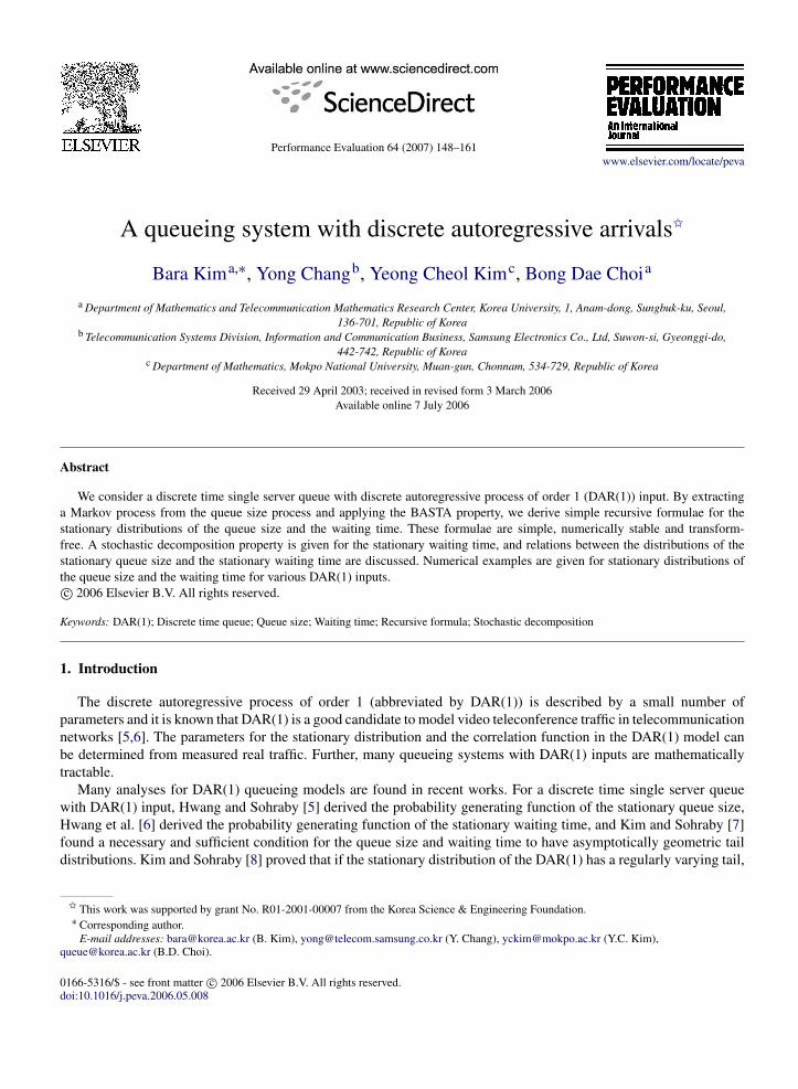
Fig. 1. DAR(1) and embedded slots.

find that the system is not empty at the arrival epoch have to wait until the server becomes available. We assume thestability condition

ρ ≡ E[B(0)] < 1.

3. Recursive formula for the queue size distribution

Let N (t) (N (t), respectively) be the number of packets in the system immediately before (after, respectively)arrivals at the beginning of the t th slot. Then the following recursions are obtained:

N (t) = N (t)+ Y (t), t = 0, 1, 2, . . . ; (2)

N (t + 1) = max{N (t)− 1, 0}, t = 0, 1, 2, . . . . (3)

The above recursions lead to a recursion for the process {N (t) : t = 0, 1, 2, . . .}

N (t + 1) = max{N (t)+ Y (t)− 1, 0}, t = 0, 1, 2, . . . , (4)

and a recursion for the process {N (t) : t = 0, 1, 2, . . .}

N (t + 1) = max{N (t)− 1, 0} + Y (t + 1), t = 0, 1, 2, . . . . (5)

Now we analyze the {N (t) : t = 0, 1, 2, . . .}. First we extract a Markov process from {N (t) : t = 0, 1, 2 · · · } byembedding at epochs t such that α(t) = 1 (Fig. 1). Define Sn , n = 0, 1, 2, . . ., by

S0 ≡ 0,

Sn ≡ inf{t > Sn−1 : α(t) = 1}, n = 1, 2, . . . .

Then, it can be easily shown that {N (Sn) : n = 0, 1, 2, . . .} is a Markov process with state space {0, 1, 2, . . .}. Let

Xn ≡ Sn − Sn−1, n = 1, 2, . . . .

Then Xn , n = 1, 2, . . ., are i.i.d. and

P{Xn = i} = (1− β)β i−1, i = 1, 2, . . . .

Since Y (t) = B(Sn) for Sn ≤ t < Sn+1, the number of packets that arrive during slots Sn, Sn + 1, . . . , Sn+1 − 1 isXn+1 B(Sn). Since the service time of a packet is one slot, the number of packets that depart the system during slotsSn, Sn + 1, . . . , Sn+1 − 1 is Xn+1 if there is no idle slot among slots Sn, Sn + 1, . . . , Sn+1 − 1. Therefore the Markovprocess {N (Sn) : n = 0, 1, 2, . . .} evolves by the following recursion:

N (Sn+1) = max{N (Sn)+ Xn+1(B(Sn)− 1), 0}, n = 0, 1, 2, . . . . (6)

Now we find the limiting distribution of {N (t) : t = 0, 1, 2, . . .} by using the Markov process {N (Sn) : n =0, 1, 2, . . .}. Actually the limiting distribution of {N (t) : t = 0, 1, 2, . . .} is the same as that of {N (Sn) : n =0, 1, 2, . . .} as we see in the following lemma.


Lemma 1. The processes {N (t) : t = 0, 1, 2, . . .} and {N (Sn) : n = 0, 1, 2, . . .} have the same limiting distributions,i.e.,

limt→∞

P(N (t) = i) = limn→∞

P(N (Sn) = i), i = 0, 1, 2, . . . .

Proof. Since the Markov process {N (Sn) : n = 0, 1, 2, . . .} is irreducible and aperiodic, limn→∞ P(N (Sn) = i) existsand

limn→∞

1n

n∑k=1

1{N (Sk )=i} = limn→∞

P(N (Sn) = i), a.s., i = 0, 1, 2, . . . . (7)

From the stability condition ρ < 1, it is easy to show that the Markov process {(N (t), Y (t)) : t = 1, 2, . . .} is ergodic.Hence limt→∞ P(N (t) = i) exists and

limt→∞

1t

t∑k=1

1{N (k)=i} = limt→∞

P(N (t) = i), a.s., i = 0, 1, 2, . . . . (8)

Now it remains to show that

limn→∞

1n

n∑k=1

1{N (Sk )=i} = limt→∞

1t

t∑k=1

1{N (k)=i}, a.s., i = 0, 1, 2, . . . . (9)

Since {α(t) : t = 1, 2, . . .} and {B(t) : t = 0, 1, 2, . . .} are independent, for each t = 1, 2, . . ., α(t) is independent ofB(0), . . . , B(t − 1), α(1), . . . , α(t − 1). Further, α(t) is independent of N (1), . . . , N (t), α(1), . . . , α(t − 1) becauseN (1), . . . , N (t) are determined by B(0), . . . , B(t − 1), α(1), . . . , α(t − 1). Thus, the process {N (t) : t = 1, 2, . . .}

satisfies the lack of anticipation assumption in Theorem 3 in Appendix with respect to the Bernoulli process{α(t) : t = 1, 2, . . .}. Therefore (9) holds by BASTA (Theorem 3 in Appendix). �

Now we derive a recursion for the limiting distribution of {N (t) : t = 0, 1, 2, . . .}. Let

πi ≡ limt→∞

P{N (t) = i} = limn→∞

P{N (Sn) = i}, i = 0, 1, 2, . . . .

By (6), we have

pi j ≡ P(N (Sn+1) = j |N (Sn) = i) =

{a j−i , if j > 0,

a−i , if j = 0,

where ak ≡ P{Xn+1(B(Sn)− 1) = k} and ak ≡∑k

l=−∞ al , k = . . . ,−1, 0, 1, . . .. By the balance equation

n∑i=0

∞∑j=n+1

πi pi j =

∞∑i=n+1

n∑j=0

πi pi j , n = 0, 1, 2, . . . ,

we have

n∑i=0

πi an+1−i =

∞∑i=n+1

πi an−i , n = 0, 1, 2, . . . , (10)

where ak ≡∑∞

l=k al , k = . . . ,−1, 0, 1, . . .. Since

a−k = P{Xn+1(B(Sn)− 1) = −k}

= P{Xn+1 = k, B(Sn) = 0}

= b0(1− β)βk−1, k = 1, 2, . . . ,

(10) leads to

n∑i=0

πi an+1−i =

∞∑i=n+1

πi b0βi−n−1, n = 0, 1, 2, . . . . (11)


By (11), we have

β

n+1∑i=0

πi an+2−i =

∞∑i=n+2

πi b0βi−n−1, n = 0, 1, 2, . . . . (12)

Subtracting (12) from (11) leads to

πn+1 =1

b0 + βa1

n∑i=0

πi (an+1−i + (1− β)an+2−i ), n = 0, 1, 2, . . . . (13)

By summing both sides of (13) over n from 0 to∞, we have

∞∑n=1

πn =1

b0 + βa1

∞∑n=0

n∑i=0

πi (an+1−i + (1− β)an+2−i )

=1

b0 + βa1

∞∑i=0

∞∑n=i

πi (an+1−i + (1− β)an+2−i )

=1

b0 + βa1

∞∑i=0

πi

((1− β)

∞∑i=1

ai + βa1

). (14)

Since∑∞

n=0 πn = 1 and

∞∑i=1

ai =

∞∑i=1

P(Xn+1(B(Sn)− 1) ≥ i)

= E[Xn+1(B(Sn)− 1) · 1{Xn+1(B(Sn)−1)>0}]

= E[Xn+1(B(Sn)− 1)] − E[Xn+1(B(Sn)− 1) · 1{(B(Sn)=0)}]

=ρ − 11− β

+b0

1− β,

(14) becomes

1− π0 =ρ − 1+ b0 + βa1

b0 + βa1,

that is,

π0 =1− ρ

b0 + βa1. (15)

By (13) and (15), the limiting distribution {πi : i = 0, 1, 2, . . .} of the {N (t) : t = 0, 1, 2, . . .} is obtained.In summary, we have the following theorem.

Theorem 1. The limiting distribution {πi : i = 0, 1, 2, . . .} of the number of packets {N (t) : t = 0, 1, 2, . . .} (beforearrivals if any) at the beginning of slots is obtained by

π0 =1− ρ

b0 + βa1, (16)

πn+1 =1

b0 + βa1

n∑i=0

πi (an+1−i + (1− β)an+2−i ), n = 0, 1, 2, . . . . (17)

Now we consider the number N (t) of packets in the system after arrivals (if any) at the beginning of the t th slot.By (3), we obtain the relations

π0 = π0 + π1 and πn = πn+1, n = 1, 2, . . . , (18)

where πn ≡ limt→∞ P(N (t) = n), n = 0, 1, 2, . . ..


The number of packets in the service position is 1{N (t)≥1} after arrivals at the beginning of the t th slot. Hence the

mean number of packets in the service position is P(N (t) ≥ 1) after arrivals at the beginning of the t th slot. Thearrival rate into the service position, which equals the arrival rate into the system, is ρ. Every packet that joins thesystem stays one slot in the service position. Therefore Little’s formula [12] yields

limt→∞

P(N (t) ≥ 1) = ρ,

which implies that

1− π0 = ρ. (19)

By (18) and (19), we obtain πn , n = 0, 1, 2, . . ., by

π0 = 1− ρ, π1 = π0 − 1+ ρ and πn = πn−1, n = 2, 3, . . . . (20)

By Theorem 1 and (20), a recursive relation for {πi : i = 0, 1, 2, . . .} is obtained as follows:

Corollary 1. The limiting distribution {πi : i = 0, 1, 2, . . .} of the number of packets {N (t) : t = 0, 1, 2, . . .} (afterarrivals if any) at the beginning of slots is obtained by

π0 = 1− ρ; (21)

πn+1 =1

b0 + βa1

((1− ρ)(an + (1− β)an+1)+

n∑i=1

πi (an+1−i + (1− β)an+2−i )

), n = 0, 1, 2, . . . . (22)

Remark. 1. The process {N (t) : t = 0, 1, 2, . . .} is stochastically equivalent to the queue size process treated in [5]because both processes evolve by the same recursion (5). Therefore the limiting distribution of the queue sizeprocess in [5] is also obtained by (21) and (22).

2. The right hand sides of (17) and (22) are computed by additions and multiplications of nonnegative numbers. Thus,the recursions (17) and (22) are numerically stable.

3. Suppose that numerical values bk, bk, k = 0, 1, 2, . . . , n + 2, and β are given, where bk =∑∞

j=k bk . Then thecomputational complexity for a1, . . . , an and a1, . . . , an is O(log n) by the following algorithm:

For k = 1, 2, . . . , n

ak ← 0

end

an+1 ← 0

for k = 2, 3, . . . , n + 1

for j = 1, . . . , bn

k − 1c

a(k−1) j ← a(k−1) j + bk(1− β)β j−1

end

an+1 ← an+1 + bkβb

nk−1 c

end

an+1 ← an+1 + bn+2

for k = n, n − 1, . . . , 1

ak ← ak+1 + ak

end

The computational complexity of the recursion for π0, . . . , πn in Theorem 1 (and the recursion for π0, . . . , πn inCorollary 1) is O(n2).


4. Waiting time distribution

In this section, we investigate relations between the queue size distribution and the waiting time distribution. Letwi , i = 0, 1, 2, . . ., be the probability that the waiting time is n for an arbitrarily chosen packet. First we derive astochastic decomposition property that the stationary waiting time can be expressed as an independent sum of thestationary number of packets and a nonnegative integer-valued random variable.

Theorem 2. Let W and N denote random variables such that

P(W = i) = wi and P(N = i) = πi , i = 0, 1, 2, . . . .

Let Φ be a random variable that is independent of N and that has a distribution given by

P(Φ = i) =1ρ

[ai + (1− β)ai+1

], i = 0, 1, 2, . . . . (23)

Then

W = N + Φ in distribution. (24)

Proof. To deal with the stationary distribution of the waiting time, we assume that the system is at steady state.Suppose that an arbitrarily chosen packet, called the tagged packet, arrives at the beginning of the t th slot. Let S bethe last epoch such that S ≤ t and α(S) = 1. Then the waiting timeW of the packet satisfies

W = N (S)+ (Y (S)− 1)(t − S)+ K ,

where K is the number of packets that arrive at the beginning of the t th slot and that receive services before the taggedpacket. Notice that N (S) and (Y (S)− 1)(t − S)+ K are independent, and that, by Lemma 1,

N (S) = N in distribution. (25)

We complete the proof by showing

P((Y (S)− 1)(t − S)+ K = i) =1ρ[ai + (1− β)ai+1], i = 0, 1, 2, . . . . (26)

Since K is independent of t − S, for k = 1, 2, . . ., and u = 0, 1, 2, . . ., we have

P((Y (S)− 1)(t − S)+ K = i |Y (S) = k, t − S = u) = P(K = i − (k − 1)u|Y (S) = k)

=

{1k, if (k − 1)u ≤ i ≤ (k − 1)(u + 1),

0, otherwise.(27)

Since Y (S) and t − S are independent and

P(Y (S) = k) =kbk

ρ, k = 1, 2, . . . ;

P(t − S = u) = (1− β)βu, u = 0, 1, 2, . . . ,

we have

P(Y (S) = k, t − S = u) =kbk

ρ(1− β)βu, k = 1, 2, . . . , u = 0, 1, 2, . . . . (28)

By (27) and (28),

P((Y (S)− 1)(t − S)+ K = i) =∞∑

k=1

∞∑u=0

bk

ρ(1− β)βu1{(k−1)u≤i≤(k−1)(u+1)}

=1ρ

P((B − 1)(X − 1) ≤ i ≤ (B − 1)X), (29)


where B and X are independent random variables such that

P(B = i) = bi , i = 0, 1, 2, . . . ;

P(X = i) = (1− β)β i−1, i = 1, 2, . . . .

By (29),

P((Y (S)− 1)(t − S)+ K = i) =1ρ

(P((B − 1)X ≥ i)− P((B − 1)(X − 1) > i))

=1ρ

(ai − P(X ≥ 2)P(B − 1)(X − 1) > i |X ≥ 2)

=1ρ

(ai − βP((B − 1)X > i))

=1ρ

(ai − βai+1)

=1ρ

(ai + (1− β)ai+1),

which is (26). �

Remark. The right hand side of (23) indeed gives a distribution because

∞∑i=0

1ρ

(ai + (1− β)ai+1) =1ρ

a0 +1− β

ρ

∞∑i=1

ai

=1ρ

(1− b0)+1− β

ρ

∞∑i=1

P(Xn+1(B(Sn)− 1) ≥ i)

=1ρ

(1− b0)+1− β

ρE[max{Xn+1(B(Sn)− 1), 0}]

=1ρ

(1− b0)+1− β

ρ(E[Xn+1(B(Sn)− 1)] + E[Xn+11{B(Sn)=0}])

=1ρ

(1− b0)+1− β

ρ

(1

1− β(ρ − 1)+

11− β

b0

)= 1.

Corollary 2. The limiting distribution {wn : n = 0, 1, 2, . . .} of the waiting time is related to the limiting distribution{πn : n = 0, 1, 2, . . .} of the number of packets (before arrivals if any) at the beginning of slots as follows:

w0 =1ρ

(a0 + (1− ρ)a1)π0; (30)

wn =1ρ

πn, n = 1, 2, . . . . (31)

Proof. Let

φn =1ρ

(an + (1− ρ)an+1), n = 0, 1, 2, . . . .

By (24),

w0 = π0φ0

=1ρ

(a0 + (1− β)a1)π0.


For n = 1, 2, . . ., by (24) again,

wn =

n∑k=0

πkφn−k

=1ρ[a0 + (1− β)a1]πn +

1ρ

n−1∑k=0

πk[an−k + (1− β)an−k+1]. (32)

By (13) and (32), we have

wn =1ρ

(a0 + (1− β)a1)πn +1ρ

(b0 + βa1)πn

=1ρ

πn . �

Remark. 1. It is verified that∑∞

n=0 wn = 1, where wn is given by (30) and (31):∞∑

n=0

wn =1ρ

(a0 + (1− β)a1)π0 +1ρ

∞∑n=1

πn

=1ρ

(1− b0 − βa1)π0 +1ρ

(1− π0)

=1ρ−

1ρ

(b0 + βa1)π0

= 1.

2. Xiong and Bruneel [13] showed

wn =πn+1

1− π0, n = 0, 1, 2, . . . , (33)

for a discrete-time G/D/1 queue with a general arrival process and unit service times. Corollary 2 can also beobtained from (33).

When the packet length has a general distribution, a similar analysis as in Section 3 can be applied for theunfinished work instead of the number of packets. The waiting time distribution can also be obtained by using avariant of Theorem 2 with the unfinished work instead of the number of packets. However, the authors have notfound a relation corresponding to (33) for this model with general packet length.

3. From Corollary 2, we derive

EW =1ρ

∞∑n=1

nπn . (34)

Observe that W is the delay of an arbitrary packet in the queue (excluding the one that is in service). Fort = 1, 2, . . ., N (t) is the number of packets in the system immediately before arrivals at the beginning of thet th slot. This is the same as the number of packets in the queue (excluding the one that may be in service) duringthe (t −1)th slot. Therefore

∑∞

n=1 nπn is the mean number of packets in the queue (excluding the service position)at steady state. Since ρ is the mean number of packet arrivals during a slot, (34) is interpreted as Little’s formulaapplied to the queue (excluding the service position). We also refer to [4].

Eq. (34) together with (20) yields

EW =1ρ

∞∑n=1

nπn+1 =1ρ

∞∑n=1

(n − 1)πn =1ρ

∞∑n=1

nπn −1ρ

∞∑n=1

πn .

Since∑∞

n=1 πn = 1− π0 = ρ, the above equation becomes

ρE(W + 1) =

∞∑n=1

nπn . (35)


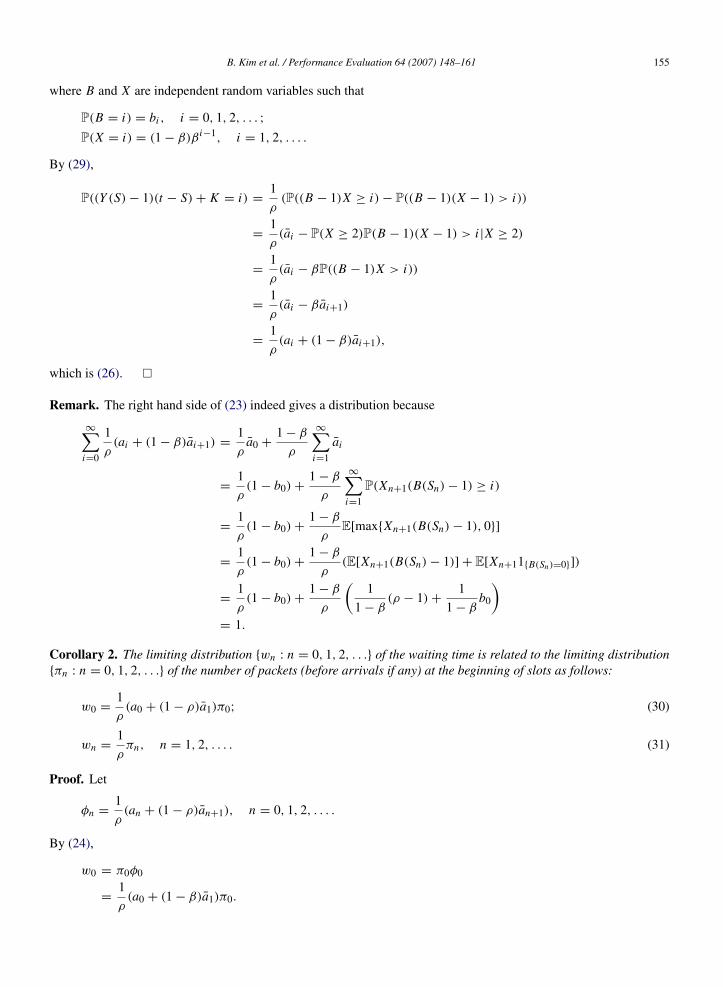
Fig. 2. Distributions of the stationary queue sizeN and the stationary waiting timeW when b0 = 1− 0.7m and bm =

0.7m .

Since W + 1 is the delay of an arbitrary packet in the system (including the service position) and∑∞

n=1 nπn isthe mean number of packets in the system (including the one that is in service) at steady state, Eq. (35) is alsointerpreted as Little’s formula (applied to the whole system).

5. Numerical examples

Fig. 2 is for the queue where β = 0.5 and the stationary distribution {bk : k = 0, 1, 2, . . .} of DAR(1) has thebinary distribution with masses at 0 and m. To get a fixed load 0.7, we set b0 = 1− 0.7

m and bm =0.7m . Fig. 2 displays

the complementary distribution functions of the stationary queue size N (before arrivals if any) at the beginning ofslots and the stationary waiting time for various values m.

The figure illustrates that the stationary queue size and the stationary waiting time increase stochastically as thevariance 0.7m−0.49 of the stationary distribution of DAR(1) increases. We observe that stationary distributions of thequeue size and the waiting time are asymptotically geometric. The figure shows that the complementary distributionof the stationary queue sizeN is close to that of the stationary waiting timeW . This is due to the relation (31) betweenthe stationary distribution of queue size and the stationary distribution of the waiting time. Eq. (31) implies that

P(W ≥ x) =1ρ

P(N ≥ x), x = 1, 2, . . . .

Hence we obtain

log P(W ≥ x) = log P(N ≥ x)+ log1ρ

, x = 1, 2, . . . . (36)

Because the second term log 1ρ

on the right hand side of the above equation is very small compared with the first termlog P(N ≥ x), log P(W ≥ x) looks very close to log P(N ≥ x) in the figure.

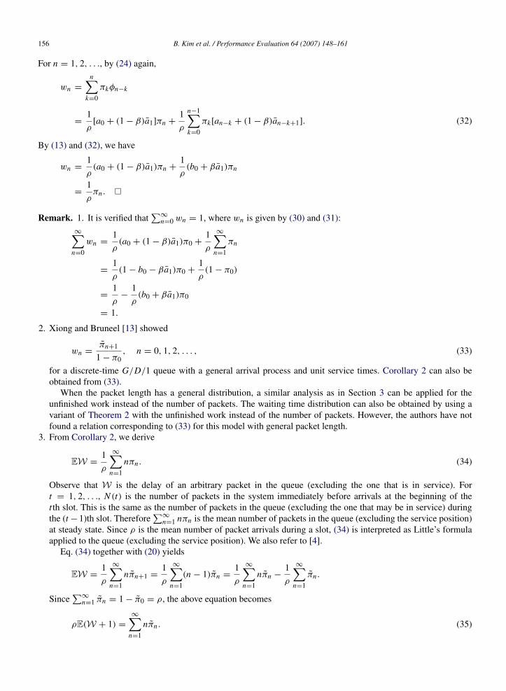
Fig. 3 is for the queue where the stationary distribution {bk : k = 0, 1, 2, . . .} of DAR(1) is geometrically distributedwith mean 0.7, i.e., bi =

1017 ( 7

17 )i , i = 0, 1, 2, . . .. Fig. 3 displays the complementary distribution functions of thestationary queue size N (before arrivals if any) at the beginning of slots and the stationary waiting time for variousdecay parameter β of the autocorrelation function of DAR(1). Notice that the larger β is, the more correlated packetarrivals are (see (1)). The figure illustrates that the stationary queue size and waiting time increase stochastically as β

increases. This is consistent with the general property: the more correlated packet arrivals are, the larger the stationaryqueue size and waiting time become stochastically. We observe that the stationary distribution of the waiting time isvery close to that of the queue size. This is due to the relation (36) as in Fig. 2.


Fig. 3. Distributions of the stationary queue sizeN and the stationary waiting timeW when bk =1017 ( 7

17 )k , k = 0, 1, 2, . . ..

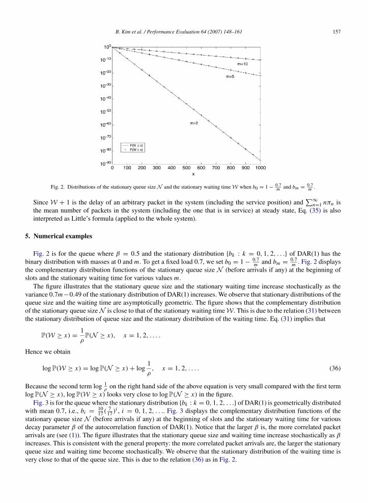
Fig. 4. Distributions of the stationary queue size N and the stationary waiting time W when bk = ck−(2+γ ), k = 1, 2, . . ., and b0 =

1− c∑∞k=1 k−(2+γ ).

Fig. 4 is for the queue where the stationary distribution {bk : k = 0, 1, 2, . . .} of DAR(1) has a heavy tail. Weset bk = ck−(2+γ ) or k = 1, 2, . . ., and b0 = 1 − c

∑∞

k=1 k−(2+γ ), and c is chosen so that the traffic load ρ is 0.7.Fig. 4 displays the complementary distribution functions of the stationary queue size N (before arrivals if any) at thebeginning of slots and the stationary waiting time for various values γ . The figure shows that the stationary queue sizeand the stationary waiting time increase stochastically as γ decreases. The figure illustrates that the stationary queuesize and the stationary waiting time have heavy-tailed distributions. We can recognize the effect of the second term onthe right hand side of (36) in the figure, because the second term is not negligible compared with the first term.

Recently Kim and Sohraby [7] proved that the stationary distribution of the queue size (and/or the stationarydistribution of the waiting time) in the DAR(1)/D/1 queue is asymptotically geometric if and only if the stationarydistribution of DAR(1) has finite support. Figs. 2–4 reflect this property. Kim and Sohraby [8] also proved that thestationary distributions of the queue size and the waiting time have regularly varying tails if the stationary distributionof the DAR(1) has a regularly varying tail. Fig. 4 reflects this property.


Appendix. Bernoulli arrivals see time averages (BASTA)

The ‘Poisson arrivals see time averages’ (PASTA) is one of the well-known properties in analyses of continuous-time queueing models. There is a discrete-time counterpart of PASTA, called ‘Bernoulli arrivals see time averages’(BASTA) or ‘Geometric arrivals see time averages’ (GASTA). A discrete-time process {An : n = 1, 2, . . .} is saidto be a Bernoulli process if it is a sequence of i.i.d. Bernoulli random variables, i.e., if A1, A2, . . . are i.i.d. withP(A1 ∈ {0, 1}) = 1. Notice that Bernoulli processes can be considered as a discrete-time counterpart of Poissonprocesses.

Many authors have applied BASTA to analyze their discrete-time queueing models (see, for examples, [1,2,11]).However BASTA does not seem to be well-known compared with PASTA. A general result of BASTA can be foundin [10]. They called the property discrete-time PASTA. Here we rewrite their result in a simple form. We also appenda proof for convenience of readers.

Theorem 3 ((BASTA) [10]). Let {Zn : n = 1, 2, . . .} be a stochastic process taking values in a measurable space(E, E) and {An : n = 1, 2, . . .} a Bernoulli process with P(A1 = 1) > 0. Suppose that the following, called the ‘lackof anticipation assumption’, holds:

An is independent of {Z1, . . . , Zn, A1, . . . , An−1} for each n = 1, 2, . . . . (37)

Define τn , n = 1, 2, . . ., by

τ1 = inf{k ≥ 1 : Ak = 1};

τn = inf{k > τn−1 : Ak = 1}, n = 2, 3, . . . .

Then, for every C ∈ E ,

1n

n∑k=1

1{Zk∈C} converges a.s. if and only if1n

n∑k=1

1{Zτk∈C} converges a.s. (38)

Further, if the convergence holds, then

limn→∞

1n

n∑k=1

1{Zk∈C} = limn→∞

1n

n∑k=1

1{Zτk∈C} a.s. (39)

Proof. Let

Mn =

n∑k=1

1{Zk∈C}(1{Ak=1} − p), n = 1, 2, . . . ,

where p = P(A1 = 1). For n = 1, 2, . . ., let Fn be the σ -field generated by Z1, . . . , Zn, A1, . . . , An . By the lack ofanticipation assumption,

E[Mn+1 − Mn|Fn] = E[1{Zn+1∈C}(1{An+1=1} − p)|Fn]

= E[E[1{Zn+1∈C}(1{An+1=1} − p)|Z1, . . . , Zn+1, A1, . . . , An]|Z1, . . . , Zn, A1, . . . , An]

= E[1{Zn+1∈C}E[1{An+1=1} − p|Z1, . . . , Zn+1, A1, . . . , An]|Z1, . . . , Zn, A1, . . . , An]

= E[1{Zn+1∈C}E[1{An+1=1} − p]|Z1, . . . , Zn, A1, . . . , An]

= 0.

Hence {Mn : n = 1, 2, . . .} is a martingale with respect to the filtration {Fn : n = 1, 2, . . .}. Since

|Mn+1 − Mn| = 1{Zn+1∈C}|1{An+1=1} − p| ≤ 1, n = 1, 2, . . . ,

the strong law of large numbers for martingale differences ( [9], p. 53, E, with bn = n) yields

limn→∞

1n

Mn = limn→∞

(1n

n∑k=1

1{Zk∈C}1{Ak=1} − p1n

n∑k=1

1{Zk∈C}

)= 0, a.s.


Therefore

1n

n∑k=1

1{Zk∈C}1{Ak=1} converges a.s. if and only if1n

n∑k=1

1{Zk∈C} converges a.s., (40)

and, if the convergence holds, then

limn→∞

1n

n∑k=1

1{Zk∈C}1{Ak=1} = p limn→∞

1n

n∑k=1

1{Zk∈C} a.s. (41)

On the other hand, since

1τn

τn∑k=1

1{Zk∈C}1{Ak=1} =1τn

n∑k=1

1{Zτk∈C} =n

τn

1n

n∑k=1

1{Zτk∈C}

and

limn→∞

n

τn= p a.s.,

we have that

1τn

τn∑k=1

1{Zk∈C}1{Ak=1} converges a.s. if and only if1n

n∑k=1

1{Zτk∈C} converges a.s., (42)

and that if the convergence holds, then

limn→∞

1τn

τn∑k=1

1{Zk∈C}1{Ak=1} = p limn→∞

1n

n∑k=1

1{Zτk∈C} a.s. (43)

It can be shown that

1n

n∑k=1

1{Zk∈C}1{Ak=1} converges a.s. if and only if1τn

τn∑k=1

1{Zk∈C}1{Ak=1} converges a.s.

Therefore (38) follows from (39), (40) and (42) follows from (41) and (43). �

References

[1] B. Desert, H. Daduna, Discrete time tandem networks of queues: Effects of different regulation schemes for simultaneous events, PerformanceEvaluation 47 (2002) 74–104.

[2] O.J. Boxma, W.P. Groenendijk, Waiting times in discrete-time cyclic-service systems, IEEE Transactions on Communications 36 (2) (1988)164–170.

[3] B.D. Choi, B. Kim, G.U. Hwang, J.-K. Kim, The analysis of a multiserver queue fed by discrete time autoregressive process of order 1,Operations Research Letters 32 (1) (2004) 85–93.

[4] D. Fiems, H. Bruneel, A note on the discretization of Little’s result, Operations Research Letters 30 (1) (2002) 17–18.[5] G.U. Hwang, K. Sohraby, On the exact analysis of a discrete-time queueing system with autoregressive inputs, Queueing Systems 43 (1–2)

(2003) 29–41.[6] G.U. Hwang, B.D. Choi, J.-K. Kim, The waiting time analysis of a discrete time queue with arrivals as an autoregressive process of order 1,

Journal of Applied Probability 39 (3) (2002) 619–629.[7] B. Kim, K. Sohraby, On the tail behavior of queues with discrete autoregressive arrivals, in: Proceedings of the 18th International Teletraffic

Congress, ITC-18, Berlin, Germany, 2003.[8] B. Kim, K. Sohraby, Tail behavior of the queue size and waiting time in a queue with discrete autoregressive arrivals, Advances in Applied

Probability (in press).[9] M. Loeve, Probability Theory II, fourth ed., Springer-Verlag, New York, 1978.

[10] A. Makowski, B. Melamed, W. Whitt, On averages seen by arrivals in discrete time, in: Proceedings of the IEEE Conference on Decision andControl, Tampa, FL, vol. 28, 1989, pp. 1084–1086.

[11] H. Takagi, Queueing Analysis–Volume 3: Discrete-Time Systems, Elsevier Science Publishers, 1993.


[12] R.W. Wolff, Stochastic Modeling and the Theory of Queues, Prentice Hall, 1989.[13] Y. Xiong, H. Bruneel, Buffer contents and delay for statistical multiplexers with fixed-length packet-train arrivals, Performance Evaluation 17

(1993) 31–42.

Bara Kim is an associate professor in the Department of Mathematics at Korea University, Seoul, Korea. He received B.S.,M.S. and Ph.D. in Mathematics from Korea Advanced Institute of Science and Technology (KAIST). During 2002 he wasa visiting scholar in the School of Industrial and Systems Engineering at Georgia Institute of Technology. His areas ofinterests include probability theory, stochastic models, applied operations research, queueing theory and their applicationsto the communication systems and industrial engineering.

Yong Chang received the B.S degree in mathematics in 1992 from HanYang University, Korea. He received the M.S degreein applied mathematics in 1994 and the Ph.D degree in applied mathematics in 1998 respectively, both from the KoreaAdvanced Institute of Science and Technology, South Korea. He was awarded the Summa Cum Laude Prize at HanYangUniversity in 1992. Since 1998, he has been at Telecommunication System Division, Information & CommunicationBusiness, Samsung Electronics Co. Ltd where he is a senior engineer. His current research interests are in the systemdesign and the air interface technologies to support 3G Long Term Evolution, IEEE802.11n, and IEEE802.16e evolution.

Yeong Cheol Kim is a professor in the Department of Mathematics at Mokpo National University, Mokpo, Chonnam,Korea. He received B.S. in mathematics in 1980 from Chonnam National University, and M.S. in 1982 in mathematics fromSeoul National University, and Ph.D. in 1998 in Mathematics from Korea Advanced Institute of Science and Technology(KAIST). His areas of interests include queueing theory and its applications to communication systems.

Bong Dae Choi is a Professor at Department of Mathematics and the Director of Telecommunication MathematicsResearch Center, Korea University, Seoul, Korea. He received B.S. and M.S. in Mathematics from Kyungpook Universityand Ph.D. in Mathematics from Ohio State University. He was awarded Seoul Culture Prize in Science in 2001. Hisareas of interests include queueing theory and its applications to communication systems. He is an editor of Journal ofCommunications and Networks. His papers have appeared in Queueing Systems, Journal of Applied Probability, IEEE,IEE, IEICE, Performance Evaluation, Telecommunication Systems, Computer Networks and others.

A queueing system with discrete autoregressive arrivals

Documents