A quasi-elliptic transformation for moving boundary problems with large anisotropic deformations

Journal of Computational Physics 192 (2003) 494–522

www.elsevier.com/locate/jcp

A quasi-elliptic transformation for moving boundaryproblems with large anisotropic deformations

Yannis Dimakopoulos, John Tsamopoulos *

Laboratory of Computational Fluid Dynamics, Department of Chemical Engineering, University of Patras, Patras 26500, Greece

Received 31 March 2003; received in revised form 1 July 2003; accepted 25 July 2003

Abstract

We have developed a quasi-elliptic set of equations for generating a discretization mesh that optimally conforms to

an entire domain that undergoes large deformations in primarily one direction. We have applied this method to the

axisymmetric problem of the transient displacement of a viscous liquid by a high-pressure gas. The liquid initially fills

completely a tube the diameter of which may be constant or change smoothly, suddenly or periodically along its finite

length. Key ingredients for the success of the proposed transformation are limiting the orthogonality requirements on

the mesh and employing an improved node distribution function along the deforming boundary. The retained or-

thogonal term along with the penalty method for the imposition of the boundary conditions overcome the inherent

restrictions of a conformal transformation, producing meshes of high quality. This term also eliminates the discon-

tinuous slopes of the coordinate lines that are normal to the free surface. These usually arise due to the harmonic

transformation around highly deforming surfaces. The mathematical anisotropy in the mesh generating equations

directly corresponds to the physical one, when the initially straight and normal to the axis of symmetry air/fluid in-

terface, at the tube entrance, develops mostly along the axial direction, generating a long, open bubble. Moreover, the

generalized node distribution imposes an optimal discretization of the bubble surface itself. Combining this scheme with

the mixed finite element method produces a powerful tool, with extended robustness and accuracy. In order to reduce

the computational cost, the resulting set of equations is solved with a non-linear, Gauss–Seidel technique and a variable

time step. Specific applications of the proposed scheme are presented.

� 2003 Elsevier B.V. All rights reserved.

Keywords:Moving boundary problems; Mesh generation; Finite element methods; Liquid displacement by gas; Adaptive time-stepping

1. Introduction

We are interested in developing accurate and efficient numerical schemes for simulating the displacement

of one fluid by another from a tube the diameter of which may be constant or may vary smoothly, suddenly

or periodically along its finite length. The deployment of such prototype geometries is necessary in order to

*Corresponding author. Tel.: +30-2610-997-203; fax: +30-2610-998-178.

E-mail address: [email protected] (J. Tsamopoulos).

0021-9991/$ - see front matter � 2003 Elsevier B.V. All rights reserved.

doi:10.1016/j.jcp.2003.07.027

Y. Dimakopoulos, J. Tsamopoulos / Journal of Computational Physics 192 (2003) 494–522 495

successfully analyze phenomena that take place in much more complicated, but often inaccessible

geometries and, thus, such schemes would have numerous practical applications. For example, there is

continuous interest in the displacement of oil from the ground using air or steam or various surfactants in

the so-called ‘‘enhanced oil recovery methods’’ or in the way pollutants and water flow and mix in the

ground. Similarly, the flow of air and vapor in the airway tubes of the lungs is modeled, aimed at exploring

conditions to facilitate pulmonary airway reopening. Moreover, such studies may be useful in modeling

potential accidents in nuclear reactors where light water may be displaced by gas after a steam explosion.

Because of its important advantages over conventional injection molding [1], we are currently interested ina polymer processing operation, the so-called gas-assisted injection molding (GAIM) in which nitrogen or

air at very high pressures are used to displace a polymer from a mold of a rather complex geometry.

Taylor [2] studied the steady development of a round-ended air column in a horizontal and extremely

long tube; its length was equal to about a thousand tube radii. A systematic experimental investigation of

this problem at even higher Capillary numbers (up to 10) was performed by Cox [3,4]. Motivated by the

slow, two-phase flow in channels of microscopic dimensions, where the driven fluid is more viscous than the

driving one and the capillary forces are important, Bretherton [5] developed an approximate solution by, in

effect, the method of matched asymptotic expansions and performed experiments to validate it. Bretherton�sanalysis has been thoroughly clarified and extended by Park and Homsy [6], while studying fluid dis-

placement in a Hele Shaw cell. Although fluid displacement by air in a capillary has been studied experi-

mentally for many years, its theoretical study has been restricted to simplified or steady state models. The

most common and convenient model for analyzing this phenomenon assumes steady motion of a semi-

infinite bubble in a tube of infinite length. Reinelt and Saffman [7] used finite differences to solve the Stokes

equations in a channel between two parallel plates or in a circular tube. To discretize the physical domain,

they applied a combination of two different grids: one curvilinear conformal to the free surface and another

one rectilinear parallel to the straight boundaries of the confining walls. The overlapping grids werestretched so that the number of grid points was greater in regions where they were needed the most. In-

terpolation was used to connect the solution between the two grids. A two-stage procedure was applied for

the solution of the problem. Beginning with an initial guess for the shape of the finger, a system of

equations equivalent to the biharmonic equation was solved. Having calculated the flow field, the shape of

the finger was updated to satisfy the normal-stress boundary condition and so on. Even so, numerical

results were reported in the range of 10�2 < Ca < 2 only. Beyond this range, the applied iterative scheme

failed to converge. Shen and Udell [8] presented a solution to the same problem, but instead of finite

differences, they followed the finite element technique, with a rather uniform mesh of points. Finite elementsolutions of the momentum and continuity equation, using also a two-stage procedure, were obtained only

for 5� 10�3 < Ca < 2� 10�1. These authors attempted to find solutions for capillary numbers greater than

0.2, but their results suffered from oscillations along the meniscus profile. They suggested that the oscil-

lations were probably caused by insufficient resolution of the flow field near the bubble front and in par-

ticular near the flow stagnation point(s). More recently, Giovedoni and Saita [9] solved simultaneously for

the flow field and the bubble shape using the spine parameterization introduced by Kistler and Scriven [10].

Inertial effects were taken for the first time into consideration. Converged solutions were obtained for

Reynolds numbers between 0 and an upper limit, which depended on Ca, whereas Ca was varied between10�4 and 10.

Very few researchers have examined the transient penetration of a bubble in a liquid-filled tube. The

main reason is the lack of robust methods for constructing meshes that highly deform with time [11]. An

attempt to solve a similar problem was made by Frederiksen and Watts [12]. They studied both the fluid

entrainment by a moving plate and the cavity flow problems using a classical finite element approximation

for the position of the internal nodes. Although their meshes were very coarse, their calculations ap-

proximated satisfactorily the actual phenomena. However, for small values of the capillary number saw

tooth instabilities covered the whole free surface of the viscous liquid. Coating flows were also examined by

496 Y. Dimakopoulos, J. Tsamopoulos / Journal of Computational Physics 192 (2003) 494–522

Sackinger et al. [13], in an attempt to test the efficiency of their combination of finite element and pseudo-

solid methods. Despite the high resolution of the contact line region there was a large shifting of the nodes

along the moving wall in dip coating, probably caused by inappropriate boundary conditions on their grid

generation scheme. More recently, they have advanced their methodology by performing three-dimensional

calculations [14,15].

Accurate simulation of moving boundary flows is a difficult and demanding task, because computing a

succession of transient states may require reconstruction of the mesh several times as the flow domain

changes in shape and size. The coupling between the instantaneous location of the interface and the fieldvariables introduces additional non-linearities through the boundary conditions imposed there. This may

be the reason that the full dynamics of the processes we are interested in have not been examined thor-

oughly. The available numerical approaches can be classified as Lagrangian, Eulerian, and mixed Lagra-

gian–Eulerian based on the method generating the computational grid. Only Eulerian techniques provide

easy handling of large interfacial distortions, because the grid points remain stationary or move in a

predetermined manner, whereas the fluid moves in and out the computational cells. This is achieved at the

expense of an interface that is not ‘‘sharply’’ defined and, consequently, the boundary conditions on it are

not as accurately approximated as the rest of the field equations. Instead, the interface is calculated basedon the values of the ‘‘color function’’ by interpolating between cells, which requires very fine meshes to

achieve certain accuracy and makes the computations very expensive, especially when the density ratio

between the two fluids is different from unity. The surface tracking method [16] is a significant improvement

for Eulerian methods because it determines the interface explicitly using a separate unstructured grid.

In the Lagrangian approach, the grid moves with the local fluid velocity (and the interface), which re-

quires frequent remeshing, but provides a sharp definition of the interface even at large deformations and

irrespective of the fluid properties. Finally, in ALE (arbitrary Lagrange–Euler) methods, kinematic de-

scriptions combine the two previous approaches, but still need a detailed technique for the mesh movement.The Lagrangian aspect of the method involves interpolation of the solution from the old to the new mesh,

which is a nontrivial and diffusive operation. This difficulty is alleviated by employing a curvilinear co-

ordinate system that conforms to the moving boundary. The evolving physical domain is mapped onto a

simple and time-independent computational one in which the moving boundary coincides with one of the

coordinate surfaces and in which it is trivial to generate the mesh. It is fairly easy to perform this boundary-

conforming mapping using simple algebraic relations [10,17,18]. However, this technique is restricted to

relatively simple initial shapes and small deformations and requires that the mapping function is single-

valued.Alternatively, elliptic mesh generation schemes in two dimensions have been proposed [19–21], which

produce the mapping between the two domains by solving two nonlinear PDEs. In spite of this additional

computational cost, the technique is preferred when more involved geometries arise, because it does not

have the limitations of the simpler algebraic methods and allows writing general codes. The quality of the

mesh to be constructed is based on the type of the mapping equation. Christodoulou and Scriven [20]

extended the earlier work by Ryskin and Leal [19] to develop a system of differential equations capable of

generating quasi-orthogonal grids, by minimizing a functional which quantifies the deviation of the mesh

from an orthogonal one that satisfies generalized Cauchy–Riemann equations. The main drawback of thisscheme was that by applying the same PDE in both coordinate directions it did not allow independent

control of mesh spacing in each direction. This was not overly restrictive, while applying this scheme for the

analysis of the slide coating flow, where the physical domain did not deform too much or preferably in one

of the directions. In contrast to this, Tsiveriotis and Brown [21] had to solve a free boundary problem in

directional solidification, where the free boundary was quite deformed and preferentially in one direction.

Typically one phase penetrated the other at distances up to three times its cross-section. They overcame this

additional difficulty by relaxing the contribution from orthogonality in the normal to the interface direc-

tion. Along the interface, nodes were equally distributed, while at the other boundaries reflective boundary

Y. Dimakopoulos, J. Tsamopoulos / Journal of Computational Physics 192 (2003) 494–522 497

conditions were used, allowing in this way the motion of the boundary nodes according to the interface

deformation. To improve the accuracy of the solution on the interface, Tsiveriotis and Brown [22] proposed

a two- to one-element splitting scheme, for a transition from a smaller number of elements in the bulk to a

larger one close to the interface. However, this splitting resulted in elements with great aspect ratios and the

generated grid lacked homogeneity; there were regions with extremely high concentration of elements and

others where the grid was rather coarse. Recently, Helenbrook [11] tried to overcome the inherent re-

strictions of the ‘‘direct’’ harmonic transformation, using a biharmonic operator. This allowed him to

specify two boundary conditions on each side of the computational domain, but as he mentioned, its maindisadvantage was the increased computational expense (about four times the cost of employing the

harmonic operator), which makes it unsuitable for large-scale calculations.

In our transient simulations we have to generate successive meshes that allow the bubble front to

eventually penetrate inside the liquid at distances even larger than 12 times the tube radius. Having

thoroughly examined the performance of the above-mentioned mesh generating techniques in our problem,

we found out that they were not satisfactory for such large deformations. Thus we developed a new elliptic

mesh generation technique, the key features of which are presented in Section 3 along with the finite ele-

ment method for solving the complete problem. Before that, in Section 2, we present the governingequations, which depend on two dimensionless parameters, the modified Reynolds number and the applied

by the gas pressure normalized by capillary forces, and various geometric ratios. Results are presented in

Section 4, where fluid displacement in straight, constricted, complex, and undulated tubes is discussed.

Finally, conclusions are drawn in Section 5.

2. Problem formulation

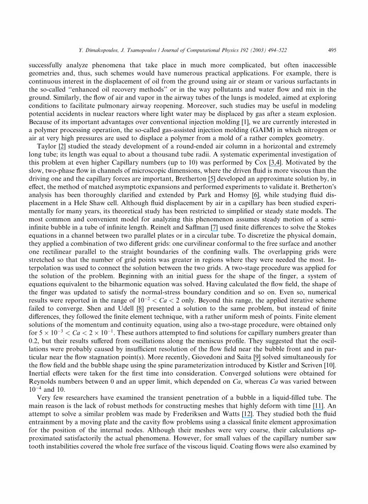
A cross-section of a prototype tube along its axis of symmetry is shown schematically in Fig. 1. In its

most general representation, the tube can be split in its entrance and exit regions, of different diameters

each, in its expansion and contraction regions, here represented by segments of sinusoidal curves and its

main region, in the middle. Each region can have different lengths. The radii of the introductory, the

Fig. 1. Schematic of a complex tube initially filled with fluid, which is displaced by high-pressure air.

498 Y. Dimakopoulos, J. Tsamopoulos / Journal of Computational Physics 192 (2003) 494–522

primary and the exit tubes are denoted as a1, a, and a2, respectively, and their corresponding lengths as b1,b, and b4, respectively. The lengths of the expansion and the contraction regions are equal to b2 and b3,respectively. Thus, the radius of this tube along its length is given by

SrðZÞ ¼

a1; 06 �ZZ6 �ZZ1;

f ðZÞ � a1 þ ða� a1Þ sin p2

�ZZ� �ZZ1�ZZ2� �ZZ1

h i; �ZZ1 6

�ZZ6 �ZZ2;

a; �ZZ2 6�ZZ6 �ZZ3;

gðZÞ � a2 þ ða2 � aÞ sin p2

�ZZ� �ZZ3�ZZ4� �ZZ3

h i; �ZZ3 6

�ZZ6 �ZZ4;

a2; �ZZ4 6�ZZ6 �ZZ5;

8>>>>>><>>>>>>:

ð1Þ

where �ZZ1 ¼ b1, �ZZ2 ¼ �ZZ1 þ b2, �ZZ3 ¼ �ZZ2 þ b, �ZZ4 ¼ �ZZ3 þ b3, �ZZ5 ¼ �ZZ4 þ b4 and an overbar indicates a dimensional

quantity. From this prototype geometry one can generate all the others that will be examined in this work.

For example, by setting b1 ¼ b2 ¼ b3 ¼ b4 ¼ 0 we obtain a straight tube and by setting b1 ¼ b2 ¼ b3 ¼ 0 we

obtain the suddenly constricted tube, etc.

Initially, the tube is filled completely with a viscous liquid, which forms a straight interface with a gas at

the tube entrance. The fluid is incompressible and Newtonian, of constant viscosity l and density q andsticks to the tube wall, forming a three-phase contact line at the entrance of the tube, which is located in the

left hand side of the tube cross-section in Fig. 1. At start up, the pressure in the air at the tube entrance is

increased abruptly from zero to �PPext, whereas the pressure at the tube exit remains at zero and displacing of

the fluid is initiated. This change causes a continuous deformation of the free surface, the position vector of

which is given by

�FF ¼ �RRer þ �ZZeZ ; ð2Þ

in the primitive representation relative to a cylindrical coordinate system centered at the axis of symmetry

of the tube, where ðer; eh; eZÞ are the corresponding unit vectors. The fluid pressure is denoted by �PPð�RR; �ZZ; �ssÞand the radial and axial component of the velocity vector in the fluid by �vvrð�RR; �ZZ; �ssÞ and �vvZð�RR; �ZZ; �ssÞ,respectively,

�vv ¼ �vvrð�RR; �ZZ; �ssÞer þ �vvZð�RR; �ZZ; �ssÞeZ : ð3Þ

We scale lengths with the radius of the primary tube, a, but, due to the accelerating nature of the flow, nocharacteristic velocity exists. Instead, we scale pressure with the externally applied, but constant air pres-

sure, �PPext, and derive a characteristic velocity assuming that Poiseuille flow takes place in a straight tube of

radius a and length Leq equal to the total length of the examined geometry, for example, Leq ¼ bþ b4 in a

constricted tube, vch ¼ ða2 �PPextÞ=ðlLeqÞ. Thus the resulting dimensionless groups are a modified Reynolds

number, which compares the applied pressure to viscous forces and the dimensionless applied pressure

relative to the capillary force. They are defined as

Rep ¼qa3 �PPextLeql2

; Pext ¼a2 �PPextrLeq

: ð4Þ

In these definitions, r is the surface tension of the air–liquid interface. In all geometries to be examined theaspect ratio, e ¼ a=Leq will arise along with additional ratios of length scales in specific geometries. For

example, in a suddenly constricted tube we will have also the contraction ratio, rc ¼ a2=a and the aspect

ratio of the main tube, a=b.The geometry in Fig. 1 has several points that may pose additional computational difficulties. They

are the three-phase contact line at the entrance of the tube, the expansion and contraction corners, and

the recirculation corners. It is well known that points where abrupt changes in geometric shape (i.e.

Y. Dimakopoulos, J. Tsamopoulos / Journal of Computational Physics 192 (2003) 494–522 499

contraction corner) and/or boundary conditions (contact line) take place are responsible for a singular

behavior of the stress tensor. Moreover, the expanding portion of the tube will provide additional area

for the bubble to move to, introducing additional complications to its shape. To handle numerically the

non-integrable stress singularity or the unexpectedly deforming bubble, a careful choice of boundary

conditions and numerical methods is needed. Although in the present formulation the contact point is

stationary due to fluid adherence at the tube entrance, fluid flow does take place in its vicinity which

can be computed only when the capillary force exerted on the moving surface is below a certain limit.

Beyond that value, all field variables are inaccurate or do not converge. This is first observed in theinterface shape, which develops a saw tooth shape between successive surface nodes. The resolution of

the flow field in such cases requires special treatment near the contact point, which is beyond the scope

of the present study, since in GAIM capillary forces are clearly subdominant to the applied pressure as

well as to viscous forces.

The Navier–Stokes equations subject to the constraint of divergence – free velocity field, for an in-

compressible fluid, govern the transient motion of a viscous fluid within the tube

RepDvDs

�r � r ¼ 0; ð5Þ

r � v ¼ 0; ð6Þ

where s is the dimensionless time, D=Ds ¼ eðo=osÞ þ v � r is the material derivative, r ¼ ðo=oRÞer þð1=RÞðo=oHÞeh þ ðo=oZÞeZ is the gradient operator and r ¼ �e�1PI þ ðrvþ ðrvÞTÞ is the total stress

tensor. Along the free surface the velocity field should satisfy a local balance between viscous stresses, n � r,surface tension, 2Hn=Pext, and gaseous pressure, e�1n:

n � r ¼ 2HPext

n� 1

en; 2H ¼ �rs � n; rs ¼ ðI � nnÞ � r: ð7Þ

In Eq. (7), 2H is twice the local mean curvature of the free surface; n is its inward unit normal, rs is the

surface gradient operator, and I is the identity tensor. Taking the inner product between Eq. (7) and the

unit tangent, t, we get the tangential stress balance

tn : r ¼ 0; ð8Þ

while acting similarly with the normal vector, Eq. (7) yields

nn : r ¼ 2HPext

� 1

e: ð9Þ

The transient free surface shape is a material surface provided that there is no mass transfer across it

DFDs

¼ v: ð10Þ

The velocity field must be also bounded at the centerline, and all variables must be symmetric around it

n � v ¼ 0; tn : r ¼ 0; FR ¼ 0: ð11Þ

Finally, the velocity field must be zero along the tube wall

vr ¼ 0; vZ ¼ 0; ð12Þ

and fully developed far downstream, where we apply hard boundary conditions [23]

500 Y. Dimakopoulos, J. Tsamopoulos / Journal of Computational Physics 192 (2003) 494–522

vr ¼ 0;ovZoZ

¼ 0: ð13Þ

The mathematical statement of the problem is completed by specifying the initial conditions. Initially, fluid

is assumed to occupy all the interior of the tube, to be under constant pressure �PP ð�RR; �ZZ; 0Þ ¼ 0, and to be

quiescent �vvð�RR; �ZZ; 0Þ ¼ 0. Its free surface in contact with the air is assumed to be flat and located at the

entrance of the tube.

3. Numerical solution

For reasons related to accuracy, flexibility, and robustness of the numerical algorithm, the resulting set

of equations is solved by a combination of an elliptic grid generation scheme and the mixed finite element

method. The use of the finite element method guarantees the accuracy and the stability of the numerical

results in each time step, while the elliptic mesh generation offers a very robust way of constructing a mesh

of points even in very deformed and evolving domains. The principle of this numerical approach has been

used [20,21] before, albeit in much less deformed or deforming domains.

3.1. Elliptic grid generation

When the grid must evolve with the solution at each time step, an inherent requirement of moving

boundary problems, a succession of mesh reconstructions, followed by interpolation of the solution vector

from the old grid to the new one must be used. To overcome this restriction, a modification of Winslow�sequations has been developed [20,21,24]. The new set of mapping equations is capable of dynamically

adapting the grid points so as to move in response to the developing free surface. The point distribution

over the domain is thus readjusted dynamically to keep a relatively uniform concentration of points in the

whole physical domain, without relying on prior knowledge of the interface location or placing unphysical

restrictions on its shape. The physical domain is mapped onto a fixed in time computational one, wherein a

simple mesh tessellation is generated. In the present problem, we chose as computational domain the

volume occupied by the viscous fluid initially. The mapping is defined as follows:

ðR; Z; sÞ!J ðn; g; ssÞ: ð14Þ

More specifically, every fluid particle being at time s at a position with coordinates (R; Z) is transformed in a

new plane with global coordinates (n; g). The new independent variables vary in the range 06 n6 1,

06 g6 e�1, 06 ss, for a straight tube, and appropriately modified for every other specific tube geometry.

Saltzman and Brackbill [24] with their pioneering work set the fundamental principles for the con-

struction of a quantitative mesh generation scheme. According to them, the three necessary characteristic

terms to describe quantitatively a mapping are: smoothness of the mapping, orthogonality and concen-

tration of the coordinate curves in the domain [25]. Algebraic techniques can control the concentration ofthe coordinate lines, but are unable to produce meshes with the other two characteristics. Even so, no

differential mapping method has been developed that accomplishes these characteristics for as large de-

formations as those anticipated in the present problem. A two-dimensional coordinate system becomes

smoother as the magnitude of the gradients of the transformed coordinates, jrnj and jrgj, decreases. Ameasure of the concentration of coordinate lines is the ratio of the area of a part of the physical domain to

the corresponding area in the transformed domain, i.e. the Jacobian of the transformation, J . Despite its

fundamental character, the analysis in [24] has limited applicability even for fixed domain problems because

the selection of three optimal scaling factors is a difficult task. Kreis et al. [26] explored this problemand concluded that poorly chosen weights may lead to a mathematically ill-posed problem. The same

Y. Dimakopoulos, J. Tsamopoulos / Journal of Computational Physics 192 (2003) 494–522 501

conclusion was drawn in moving boundary problems [23]. So in contrast to what initially was recom-

mended, Christodoulou and Scriven [20] introduced the ratio, S ¼ffiffiffiffiffiffiffiffiffiffiffiffiffiffiffiffiffiffiffiffiffiffiffiffiffiffiffiffiffiffiffiffiffiffiffiffiffiffiffiðR2

n þ Z2nÞ=ðR2

g þ Z2g

qÞ, of scale factors

and its inverse, S�1, for generating the g- and n-level curves, respectively, along with an arbitrary loga-

rithmic term in order to regularize the orthogonality functional which is related to the Cauchy–Riemann

equations. A variety of combinations and modifications of the above characteristics have been proposed[25]. In our extensive numerical experiments we found out that the logarithmic term did not offer any

improvement in generating the mesh, but including S did so. Moreover, we found out that we need not

include a term affecting the concentration of mesh lines, this could be accomplished through the related

boundary conditions, see below. Apparently, Tsiveriotis and Brown [21] reached similar conclusions.

Furthermore, one must force the coordinate lines, which are parallel to the deforming interface (n-curves, having constant g-values) to follow it in its large deformations and even concentrate near it without

the strong requirement that they remain orthogonal to the rest of the boundaries, [21]. On the other hand,

the coordinate lines normal to the interface (g-curves) must meet them smoothly and orthogonally. Thusanisotropy of the mapping equations is generated, which proved to be valuable and directly corresponds to

the physical anisotropy of the deformation: the arc length of the free surface often exceeds its original size

by many times, while deforming in the direction of its original normal vector. Additional systematic tests

have demonstrated that we should not include either a different scaling in the Laplacian or add a forcing

term in its right hand side in the equation generating the n-coordinates, see also [21]. Therefore, the elliptic

equation set that performed the best in our highly deforming case is

r � e1

ffiffiffiffiffiffiffiffiffiffiffiffiffiffiffiffiR2n þ Z2

n

R2g þ Z2

g

s þ ð1� e1Þ

!rn ¼ 0 ðequation generating the g-curvesÞ; ð15Þ

r � rg ¼ 0 ðequation generating the n-curvesÞ; ð16Þ

where the subscripts indicate differentiation with respect to that variable and e1 is an empirically chosen

parameter ranging between 0 and 1 and it usually equals 0.1. The gradient operator is still defined in the

physical domain as in Section 2.

In the hypothetical presence of an orthogonality term in the (n-curves), mesh spacing becomes overly

restrictive and the imposition of the boundary conditions is not possible for all the boundaries without

destroying mesh smoothness. Indeed, numerical experiments have shown that when an orthogonal term

is present in Eq. (16), two distinct regions of mesh distribution in the physical domain develop, which

are separated by a transition zone of highly distorted elements. This is illustrated in Fig. 2 with a se-quence of meshes generated according to the Christodoulou and Scriven [20] orthogonal transformation

and initially using as boundary conditions equidistribution of nodes on all the boundaries with an

optimally defined arc length on the free surface. More on the boundary conditions that should ac-

company Eqs. (15) and (16) will be presented shortly. To keep the plots clearer, we depict rectangular

and not triangular elements, but this does affect our conclusions in any way. The flow parameters are

Rep ¼ 0, Pext ¼ 8333, and e�1 ¼ 12, and the snapshots have been taken at s ¼ 0:555, 1.3536, and 1.7493.

Due to the additional orthogonality constraint, which tries to enforce that the angle between the n- andg-coordinates is nearly 90�, even the boundary constraint on the axis of symmetry had to be relaxed tosimple orthogonality there. Otherwise, the mesh generation scheme would be overly restrictive, leading

to failure the Newton–Raphson iterations either from the very beginning or after a few time-steps. In

other words, we did not impose any condition on the distance between nodes along the axis of symmetry

(i.e. equidistribution), allowing it to increase or decrease. Alternatively, one could act similarly on the

free-surface or the tube wall, but such a change would have had an extremely destructive impact on the

mesh. The negative effect of the orthogonal term becomes visible from the beginning of the simulation,

Fig. 2(a), when the size of the bubble is small, by the nonuniformity of the mesh around the bubble. At

Fig. 2. Mesh deformation at s ¼ 0:555, 1.3536, and 1.7493, for flow parameters ðRep; Pext; e�1Þ ¼ ð0; 8333; 12Þ. The mesh has been

constructed using the geometric transformation of [20] with 40� 80 radial and axial elements, respectively, and es ¼ e1 ¼ e2 ¼ 0:1. On

the axis of symmetry, the equidistribution condition was dropped; its application would lead to an over specified system of equations,

because of the orthogonality constraint in both equations in the bulk.

502 Y. Dimakopoulos, J. Tsamopoulos / Journal of Computational Physics 192 (2003) 494–522

larger deformations two distinct regions are apparent, one surrounding uniformly the free surface (I) and

another one with element sides nearly perpendicular to the wall (II). The zone between them is occupiedby highly distorted rectangular elements with their interior angles varying from nearly 0� to 180�,making the Jacobian of the domain transformation nearly singular. The line separating the distorted

from the regular elements-close to the tube wall is quite corrugated. Additionally, the aspect ratio of

the elements in region I is large, while that of region II is small. All these make apparent why the

orthogonality requirement in the n-curves is inappropriate for the deep-penetration problems studied

herein.

It may seem awkward that, although the computational domain is simpler and is in fact used to readily

construct a simple mesh in it, the equations generating the coordinate lines in physical space are writtenwith the pair of ðn; gÞ as unknowns! The reason for that is that the corresponding mapping ðR; ZÞ ! ðn; gÞ ispreferred because it is one-to-one provided that the curvature is non-positive and the boundary convex in

the computational domain, something that can be achieved by its construction [27], whereas this is not

always guaranteed if the dependent and independent variables are exchanged in Eqs. (15) and (16), see

[19,25]. Moreover, Mastin and Thompson [28] have shown that the mapping generated by the Winslow

system [29] which does not include any orthogonal term have a strictly positive Jacobian for a uniform

mesh. When the physical domain is not convex, adding internal restrictions on the nodes solves this

problem and this is something we had to employ in the constricted tube calculations, see Section 4.2. ThenEqs. (15) and (16) can be inverted to obtain Rðn; gÞ and Zðn; gÞ, i.e. the coordinate lines in the physical

domain. Moreover, the governing equations, Eqs. (5)–(13), and the mesh generating equations, Eqs. (15)

and (16), are written in the physical domain with independent variables ðR; ZÞ, so, in general, we need to

transform them in the computational one. This procedure, although straightforward, adds to the com-

plexity of the formulation by introducing new spatial and temporal derivatives in the governing equations

according to the chain rule of differentiation

Y. Dimakopoulos, J. Tsamopoulos / Journal of Computational Physics 192 (2003) 494–522 503

o

oR¼ on

oRo

onþ ogoR

o

og;

o

oZ¼ on

oZo

onþ ogoZ

o

og; ð17Þ

o

os¼ o

ossþ on

oso

onþ og

oso

og:

In these expressions, clearly time is independent of either the original or the mapped coordinate system,

s ¼ ss, so that os=oR ¼ os=on ¼ 0, etc. and the coefficient of the time derivative o=oss is unity. Moreover, the

partial differentiations, e.g. on=os, are implied under constant location in the physical space making these

derivatives nonzero. Obviously, the partial time derivatives of the coordinates in physical space are nonzeroas well. In these expressions the derivatives of the mapped domain coordinates with respect to those in the

physical domain must be expressed in an inverse manner. This is readily accomplished and, for example, we

obtain

nR ¼ Zg

jJ j ; nZ ¼ �Rg

jJ j ; ns ¼RgZs � ZgRs

jJ j ; where jJ j ¼ RnZg

�� � RgZn

��: ð18Þ

3.2. Boundary conditions

The quality of the mesh to be constructed depends not only on the bulk equations, but also on the

boundary conditions that go along with them. Appropriate boundary conditions for Eqs. (15) and (16) are:

(a) on fixed parts of the boundary (tube walls, axis of symmetry and the exit of the tube) the equation thatdefines the boundary curve replaces the mesh generation equation associated with the coordinate that is

constrained on that boundary, and (b) the angle formed between the boundary and the mesh lines inter-

secting it. These correspond to the streamline-velocity potential couple in flow problems or to the tem-

perature-heat flux couple in heat transfer problems. However, as we will demonstrate shortly, in order to

generate an acceptable mesh one needs to control the node distribution on the boundary. This is achieved

by imposing for the type (b) boundary conditions, orthogonality between the mesh lines and the boundary

lines and adding to them the constraints described below, upon multiplication by a large (penalty) pa-

rameter, because these constraints are not natural for this problem. Thus, only the latter are effectivelyadded to the bulk equations at elements on the domain boundary. Introducing them independently would

lead to divergence of the iterative scheme.

These boundary constraints should be imposed on the dependent variables of Eqs. (15) and (16), i.e. on nor g. For example, on the axis of symmetry, n ¼ 0;R ¼ 0, and the equidistribution of nodes would require

gZZ ¼ 0. However, the mesh in the computational domain is constructed algebraically (see end of this

section) and we need instead to relate it to that in the physical domain. So we transform these requirements

to equivalent ones in the physical domain. Using the chain rule transformations similar to those given by

Eq. (17) one may show that this is equivalent to

Zgg ¼ 0; ð19Þ

where this equation requires that along the boundary increments of the arc length always vary in the

physical domain as they do in the computational one. In the same boundary the second boundary condition

sets the location of the boundary, R ¼ 0. At the free surface, the boundary condition for the g-equation, onwhich it is mapped (g ¼ 0), is the kinematic condition, Eq. (10). The requirement of node equidistribution

504 Y. Dimakopoulos, J. Tsamopoulos / Journal of Computational Physics 192 (2003) 494–522

for the n-equation should be nss ¼ 0, but again, because on this boundary, n is only a function of s and vice

versa, then d=ds ¼ ðdn=dsÞðd=dnÞ and it is straight forward to show that this is equivalent to snn=sn ¼ 0 or

d2sðnÞdn2

¼ 0; where sðnÞ ¼Z n

0

ffiffiffiffiffiffiffiffiffiffiffiffiffiffiffiffiffiffiffiffiffiffiffiffiffiffiw1R2

n þ w2Z2n

qdn and w1 þ w2 ¼ 2: ð20Þ

sðnÞ is a weighted arc length along the free surface and w1;w2 are weight parameters, which have to be

adjusted by trial and error to optimize performance. Previous researchers [20,21] used an equidistribution

condition on the free surface (w1 ¼ w2 ¼ 1), which is useful and accurate only when the deformation of the

free surface is not very large. In our case Zn becomes much larger than Rn, and their scheme produces

unsatisfactory results. So we must use weights such that w1 � w2, in order to counterbalance the previouslymentioned large disparity in the derivatives and prevent strong repulsion of the nodes from the tip of the

bubble or from the neighborhood of the contact line, where the curvature of the surface is large. On the

boundaries except for the moving surface, Tsiveriotis and Brown [21] used the condition that the respective

coordinates intersect them orthogonally. This being a weak condition could smooth out irregularities in the

node distribution. However, we found out that this is not a good choice for the present problem. Indeed,

Fig. 3(a) and (b) show that applying this condition on all boundaries except for the free surface, where node

equidistribution is applied, results in strong repulsion of nodes from the contact line, an area that needs

high resolution. At later times, not shown here, there is stronger repulsion of nodes from the bubble tip aswell making even the bubble shape nonphysical. As a final unsuccessful attempt we show in Fig. 3(c) the

mesh generated following [20] with orthogonality boundary conditions applied on all boundaries. We

observe that in addition to the strong repulsion of nodes from the contact line, the highly distorted elements

near the free surface cause node-by-node oscillations on it.

For constructing the mesh in the computational domain a bottom-up algebraic technique is adopted. If

the computational domain is still somewhat complicated, it is split in even simpler subdomains. Mesh

tessellation takes place in these subdomains introducing equidistant nodes in both directions in the com-

putations domain irrespective of the particular geometry that we examine herein. Then, the subdomains arepatched together and double nodes are removed as described in [30].

3.3. Mixed finite element method

The coordinate lines in the computational domain generate rectangular elements, which in turn are

halved to eventually create triangular elements. These, when mapped to the physical domain, were found to

better conform to its large deformations. The mixed Galerkin finite element method was used following the

work by Poslinski et al. [17,18] for viscous free-surface problems. With the term �mixed� we imply using

higher order polynomials to interpolate the velocity field than the pressure in order to comply with the

Babuska-Brezzi condition [31]. In particular, the velocity field of the viscous fluid is represented by qua-

dratic Lagrangian polynomials, /i, the pressure and the position vectors of the mesh points by linear

Lagrangian polynomials, wi and vi, respectively (6/3 formulation [30])

v ¼XNi¼1

/ivhi ;

P ¼XMi¼1

wiPhi ; ð21Þ

G � ðR; ZÞ ¼XKi¼1

viðRhi ; Z

hi Þ:

Fig. 3. Meshes generated with ðRep; Pext; e�1Þ ¼ ð0; 833; 12Þ with the following methods: (a, b) using 28� 60 radial and axial nodes and

Eqs. (15) and (16) and orthogonality BCs except at the free interface where equidistribution is used with w1 ¼ w2 ¼ 1 at s ¼ 0:288

(Ztip ¼ 1) and 0.772 (Ztip ¼ 3), respectively, and (c) using 40� 80 radial and axial nodes and following the method in [20] and or-

thogonality BCs on all boundaries at s ¼ 0:347 (Ztip ¼ 1:21). For clarity we show only half of the length of the tube and rectangular

elements.

Y. Dimakopoulos, J. Tsamopoulos / Journal of Computational Physics 192 (2003) 494–522 505

where vhi , Phi , and (Rh

i ; Zhi ) are the dependent on the mesh nodal values of velocity, pressure, and position

vector, and N , M , and K are the number of equations, for the above referred quantities. The mixed for-

mulation combined with subparametric domain representation forms a stable and economical scheme that

satisfies automatically the no-penetration or reflective conditions on all boundaries, except on the free

surface, and conservation of mass on each element.

Galerkin�s principle is invoked in order to convert the governing partial differential equations to or-dinary ones; the momentum and continuity equations are weighted with the quadratic, /i, and linear, wi,

basis functions, respectively, and then integrated over the control volume, that is the volume of the viscous

fluid.

RM ¼ /i;RepDvDs

� �� ð/i;r � rÞ ¼ 0; ð22Þ

506 Y. Dimakopoulos, J. Tsamopoulos / Journal of Computational Physics 192 (2003) 494–522

RC ¼ ðwi;r � vÞ ¼ 0: ð23Þ

Eqs. (22) and (23) are the weak forms of the momentum and continuity equations, respectively. By ð�; �Þ isdenoted the inner product defined in the whole physical domain

ðj; kÞ ¼ZVjðn; gÞkðn; gÞdV ; ð24Þ

where dV is given by dV ¼ RJ dndg, and J is defined by Eq. (18). A similar inner product arises upon

application of the divergence theorem on Eq. (22). Its definition involves a surface integral over part of the

boundary

hj; ki ¼ZAjðn; gÞkðn; gÞdA: ð25Þ

The locations of the mesh points continuously change in time, therefore the time derivatives in the

momentum equation, Eq. (5), must be transformed according to the following relationship, which isequivalent with the last of Eq. (17):

ovos

����R;Z

¼ _vv���n;g

� _GG���n;g

� rv; ð26Þ

where the dots over the symbols indicate differentiation with respect to time. The last term in Eq. (26) is an

additional convective term due to the motion of the nodes. The momentum equation involves the diver-

gence of the stress tensor (r � r) and requires application of the divergence theorem within each element in

order to reduce the order of the velocity derivatives from two to one. The resulting line integrals cancel each

other within the control volume, whereas on fluid boundaries they are either omitted in order to impose

essential conditions, i.e. no slip, no penetration at the solid wall, symmetry condition at the centerline, or

computed by the free surface stress balance. The mean curvature has to be specially treated as it involves

products of the free surface position with its second derivative. Using the methodology proposed byRuschak [32] and applied by Poslinski and Tsamopoulos [17], the mean curvature on the free surface is split

into two parts. The first term is the derivative of the tangent vector, t, of the free surface with respect to its

arc length (s), while the second part is composed of the normal vector multiplied by the inverse of the

second principal radius, R2 ¼ RffiffiffiffiffiffiffiffiffiffiffiffiffiffiffiffiR2n þ Z2

n

q=Zn,

2Hn ¼ dtds

þ nR2

; ð27Þ

where t is given as t ¼ ðRner þ ZneZÞ=ffiffiffiffiffiffiffiffiffiffiffiffiffiffiffiffiR2n þ Z2

n

qand n is equal to n ¼ ðRneZ � ZnerÞ=

ffiffiffiffiffiffiffiffiffiffiffiffiffiffiffiffiR2n þ Z2

n

q.

Introduction of Eqs. (26) and (27) into the weak form of momentum equation eventually results in

RM ¼ ð/i;Rep½ _vvþ ðv� _GGÞ � rv�Þ þ ðr/i; rÞ � d/i

ds; P�1

ext t� �

� /i;nR2

� �¼ 0: ð28Þ

Similarly, the weak forms of the mapping equations are derived by multiplying them with the vi basisfunctions

RMR ¼ vi;r � e1

ffiffiffiffiffiffiffiffiffiffiffiffiffiffiffiffiR2n þ Z2

n

R2g þ Z2

g

s þ ð1� e1Þ

!rn

!¼ 0; ð29Þ

RMZ ¼ ðvi;r � rgÞ ¼ 0: ð30Þ

Y. Dimakopoulos, J. Tsamopoulos / Journal of Computational Physics 192 (2003) 494–522 507

Applying the divergence theorem, we get

RMR ¼ rvi; e1

ffiffiffiffiffiffiffiffiffiffiffiffiffiffiffiffiR2n þ Z2

n

R2g þ Z2

g

s þ ð1� e1Þ

!rn

!¼ 0; ð31Þ

RMZ ¼ ðrvi;rgÞ ¼ 0; ð32Þ

where the integrated out terms are not included because we weakly impose orthogonality between the mesh

lines and the domain boundaries on all boundaries and we add conditions on the node distribution through

a penalty method [20]. For example, the node equidistribution condition on the free surface the boundary isimposed by

RMR��g¼0

¼ rvi; e1

ffiffiffiffiffiffiffiffiffiffiffiffiffiffiffiffiR2n þ Z2

n

R2g þ Z2

g

s þ ð1� e1Þ

!rn

!þ L

dvi

dn;dsdn

� �¼ 0; ð33Þ

where the penalty parameter is L ¼ Oð103–105Þ. Even Eqs. (19) and (20) are treated as essential conditions

after multiplication by 1i, the one-dimensional linear basis functions, and integration by parts. Finally, the

equivalent algebraic form of the kinematic differential equation is

RK ¼ 1i;DFDs

�� v�

¼ 0: ð34Þ

Alternatively it could be stated that the free surface corresponds a surface with constant isoparametric

coordinate g ¼ 0 [19], and write

RK ¼ 1i;DgDs

� �¼ 0; ð35Þ

which is equivalent to Eq. (34). Starting from either one of Eqs. (34) or (35) and applying the chain rule of

differentiation, we readily deduce that

RK ¼ h1i;RsZn � RnZs þ Rnvz � Znvri ¼ 0: ð36Þ

According to some investigators (e.g. [33]) a SUPG weighting of the kinematic condition must be usedbecause of the wave nature of Eq. (36). This is indeed the case for high order polynomial approximations of

the free surface, but in our case it is unnecessary because we employ approximation functions of low degree.

All the above integrals are evaluated numerically by Gaussian quadrature. For triangular elements a seven-

point formula was used to evaluate two-dimensional integrals and a three-point formula for one-dimen-

sional integrals.

In order to integrate accurately the governing equations in time, the implicit Euler method, which is an

A-stable approximation, with time stepping adaptation, is used. More specifically, if by oj=os ¼ f ðjÞ wedenote the set of equations to be integrated, its approximate form, using backward finite differences is

jnþ1 � jn

snþ1 � sn¼ f ðjnþ1Þ; ð37Þ

where the index n indicates the previous time instant. The difference snþ1 � sn defines the current time step

Dsnþ1. The strategy for changing the time step is based on the estimation of the local truncation error, which

is the difference between the accurate approximation jn, and an explicitly predicted one jpn:

jp ¼ j þ Ds _jj ; ð38Þ

508 Y. Dimakopoulos, J. Tsamopoulos / Journal of Computational Physics 192 (2003) 494–522

Dsnþ1 ¼ Dsnednk k

� �1=2

� Dse; ð39Þ

where e is a user defined tolerance, k � k stands for the Euclidean norm and dn ¼ jn � jpn, is the difference

between the predicted and the accurate solution at sn [34].

The resulting set of non-linear equations is solved by the modified Newton–Raphson iteration scheme

from an initial estimate corresponding to the solution of the prediction step, Eq. (38). The modified Newton

method proceeds by not updating after each iteration the Jacobian matrix and its LU decomposition, but

only after a criterion of decreased convergence rate is exceeded. The entries of the Jacobian matrix are built

up as sums of contributions from the element-level Jacobian, which is calculated by analytical differenti-

ation. The agreement of successive iterates to within a prescribed numerical tolerance, typically 10�9, was

the criterion for convergence. The large system of algebraic equations arising at each step of the Newtoniterations was solved by Gaussian elimination using a banded matrix solver.

Although the above numerical scheme guarantees the convergence to a solution at each time step, and

can be easily embedded in a typical finite element code, it is extremely memory demanding. Therefore, a

different scheme was adopted in order to decouple the mesh generation problem from the flow problem,

[35]. In particular, the total set of equations

Resðv; p;GÞ ¼ 0 ð2N þM þ 2K unknownsÞ ð40Þ

is split in two sets and each set is solved by Newton–Raphson iterations until convergence. The first set

consists of the mass and momentum balances (Eqs. (23) and (28)) and their boundary conditions

Rvesðvj; pj;Gj�1Þ ¼ 0 ð2N þM unknownsÞ; ð41Þ

while the second set consists of the mesh generating equations (Eqs. (31) and (32)) and their boundary

conditions

Rmesðvj; pj;GjÞ ¼ 0 ð2K unknownsÞ: ð42Þ

Thus the complete scheme is a Gauss–Seidel (or Picard) iteration type scheme in which for a given physicaldomain, G ¼ Gj�1, the flow problem is solved first (stage I), and once velocities and pressure have been

calculated, the mesh points are moved (stage II). The basic advantage of the method is that it generates

significantly smaller Jacobian matrices, which can be allocated and deallocated whenever needed. The

convergence of the whole scheme is ensured by the automatic time adaptation, because the predicted so-

lution does not differ too much from the exact one and the Newton/Kantorovich sufficient condition is

satisfied, [36]. It must be mentioned that in order to improve the effectiveness of the scheme and disallow

unreasonable increases of the time step, an upper bound is placed on the latter by the number of Picard

iterations. So the new time step, Dsnþ1, is determined by

Dsnþ1 ¼ minðDsp;DseÞ; ð43Þ

where Dse stands for the predicted time step (Eq. (39)) using forward Euler technique [34], whereas Dsp isgiven by

Dsp ¼ Dsndesired number of Picard cycles

actual number of Picard cycles

� �1=4

;

and Dsn is the time step in the previous instant. Usually, the desired number of Picard iterations is equal to

the actual ones at the first integration step increased by 3–4.

Y. Dimakopoulos, J. Tsamopoulos / Journal of Computational Physics 192 (2003) 494–522 509

In addition, the proposed scheme assists in readily imposing boundary conditions that depend on the

location of a particular point of the physical domain (e.g. its distance from the three-phase contact point,

when a Navier slip condition is employed) without increasing the bandwidth of each submatrix, reduces the

calculation of matrix entries and expedites checking their correctness. Moreover, for the flow problem (and

not for the mesh generation one) it is not necessary to apply the chain rule once the coordinate points of the

physical domain are given. Finally, it must be mentioned that both full Newton–Raphson and Block

Gauss–Seidel/Newton–Raphson methods have been numerically implemented and compared. Their exe-

cution times do not differ too much, with the NR method being typically 10% faster, since the GS/NRrequires about five Picard cycles per time step. So, the GS/NR should be preferred for the reasons men-

tioned above.

The program was written in Fortran 90 and run on an Alpha Dec DS20E workstation at the laboratory

of Computational Fluid Dynamics. Depending on the parameters and the type of the tube geometry, ac-

curacy of the results was tested by mesh refinement and required different size of mesh, but it typically took

about 1 day to complete a run.

4. Results and discussion

The transient flow generated by the penetrating bubble and the bubble shape are functions of the

modified Reynolds number, the dimensionless applied pressure, and the geometric ratios characterizing the

tube. The most general form of a tube section that we consider in this work is given in Fig. 1, and its various

particular simplifications will be given in each subsection that follows.

4.1. Straight tube

As we mentioned in Section 2, the complex tube geometry defined by Eq. (1) reduces to a straight one by

setting b1 ¼ b2 ¼ b3 ¼ b4. The sequence of plots shown in Fig. 4 illustrates the deformation of the dis-

cretized into triangular elements physical domain, which is generated by a uniform mesh in the compu-tational domain at s ¼ 0:65, 1.20, and 1.80. For clarity the elements are shown as rectangular, i.e. before

dividing each one of them into two triangles. We observe that, even in the cases with the largest penetration

of the air bubble, the grid retains acceptable uniformity, in contrast to the one shown in Fig. 2, which was

obtained under similar values of the physical parameters, but not following our new scheme. The mesh here

deforms smoothly and nicely following the deformation of the free surface. Regions of particular interest,

which need special attention, such as the contact line region and the front of the bubble, are handled very

effectively. In this case we have Rep ¼ 0, Pext ¼ 833, and e�1 ¼ 12 and we have set the boundary control

parameters, w1 and w2, equal to 20/11 and 2/11, respectively. Doing so, we overcame the difficulty of thelarge Zn derivative compared with Rn, which is known to cause node repulsion along the n-direction. Tosimulate accurately the above-described phenomenon, the computational domain was subdivided into a

uniform mesh by 37 nodes in the n-direction and 81 nodes in the g-direction, resulting in 5760 triangular

elements and 32,497 unknowns including the coordinate locations of the mesh points. The initial time

increment was set at Ds ¼ 0:5� 10�5.

From the physical point of view, we observe that the initially flat air/fluid interface deforms everywhere,

but mostly around the axis of the tube initially forming a wedge-like profile. Already at s � 0:544 the

bubble shape has turned into almost parabolic. Subsequently, most of the bubble front assumes a per-manent, finger-like shape with a parabolic tip and straight sides leaving behind a layer of fluid of constant

thickness, which is attached to the tube wall. Near the tube entrance the film has a small, but monotonically

increasing thickness at all times. When the bubble front reaches the length of one and a half diameters, it

attains a constant thickness. This thickness is equal to h1 ¼ 0:6325 and the liquid volume fraction

Fig. 4. The deformation of the mesh points at s ¼ 0:544, 1.334, and 1.774. The discretization is finest at the fingertip, since both the

local capillary number and the curvature are large there. ðRep; Pext; e�1Þ ¼ ð0; 833; 12Þ.

510 Y. Dimakopoulos, J. Tsamopoulos / Journal of Computational Physics 192 (2003) 494–522

remaining attached to the tube wall, which is defined as m ¼ 1� h21, is 0.60. These values have been ob-

served experimentally by Taylor and Cox [2–4], when they studied the displacement of very viscous fluids at

their higher Capillary numbers (i.e. Ca � 2–10, asymptotic region of their m vs Ca plot). Their experiments

were carried out in very long tubes and they neglected the initial transients and the tube entrance effects.

4.2. Constricted tube

The methodology we presented needs only small modifications in order to extend the simulations to

cover cases where the bubble enters a secondary tube of smaller diameter than that in the primary one. Now

it is anticipated that the bubble radius will decrease as it tries to squeeze through the contraction and the

bubble may attain a concave shape. This is not desirable, if the mapping we used is to be preserved

throughout the simulations [27]. So we need to introduce an internal constraint on the nodes right at theentrance of the secondary tube. In particular, instead of the n-component of the mesh generation set of

equations, which is dropped, the nodes are forced to obey a generalized distribution similar to that given by

Eq. (20) at the entrance of the secondary tube in the physical domain. Now the nodes in both tubes

translate following the deformation of the free surface. Thus, the nodes originally located at the vertical

boundary between the two tubes translate and rotate with respect to the contraction corner, so that an

optimal node distribution is achieved. Some indicative results of the generated mesh before, during and

after the bubble penetration in the secondary tube are shown in Fig. 5. A short primary tube, b=a ¼ 5, with

a 4:1 contraction ratio and dimensionless length of the secondary tube b4=a ¼ 4 is at s ¼ 0 filled with liquid.The applied pressure and the other liquid properties are such that Rep ¼ 0, Pext ¼ 104. To accurately sim-

ulate the penetration of air through the viscous fluid, a mesh of 13,160 triangular elements is used resulting

in 73,757 unknowns. The sequence of finite element meshes in the displaced liquid as well as the bubble

shape is shown at different time instances. At s � 131 the bubble nearly exceeds in length three radii of the

primary tube and its front surface is nearly parabolic. At s � 189 the bubble tip reaches the entrance of the

secondary tube and becomes very pointed as gas and liquid try to squeeze through the contraction

Fig. 5. Sequence of finite element meshes in the liquid that is being displaced by the gas, at s ¼ 131:32, 189.67, and 193.14 corre-

sponding to Ztip ¼ 3; 5; 6:5 with ðRep; Pext; e�1; b4=a; a2=aÞ ¼ ð0; 104; 9; 4; 0:25Þ. For clarity of the figure we have used only 44� 53 and

11� 42 radial and axial nodes in the primary and the secondary tubes, respectively. This results in 5588 triangular elements and 11,455

total nodes.

Y. Dimakopoulos, J. Tsamopoulos / Journal of Computational Physics 192 (2003) 494–522 511

generating a locally extensional flow of the liquid. Soon after entering the narrower tube, the bubble front

expands again and eventually its front becomes parabolic again. A new, narrower finger is formed thatcontinues to travel inside the secondary tube, but with a greater speed (s ¼ 191). In the neighborhood of the

contraction corner, the bubble width remains very small, ab ¼ 0:065a. As the bubble occupies more and

more space in the secondary tube, its radius seems to reach the asymptotic value of 0:156a or 0:624a2, whichcorresponds to a remaining liquid fraction in the secondary tube m ¼ 0:61, nearly Cox�s [3] value for a

straight tube, although the length of the secondary tube and, thus, the fluid resistance here are not enough

to give the bubble a constant velocity. Apparently the mesh has all the desired qualities: uniform distri-

bution of nodes throughout, bound ratio of the element sides, and dynamically adjustable nodal positions

as the free surface deforms greatly. Details of the mesh around the contraction corner for times corre-sponding in cases that the bubble has either come very close to its entrance (s ¼ 185:45) or even penetrated

in the secondary tube (s ¼ 193:94) are shown in Fig. 6(a) and (b).The bounds of the zoomed area are

46 Z6 6. Using this method, we have studied the flow of Newtonian and viscoplastic fluids in straight and

constricted tubes [37,38].

In order to demonstrate the superiority of the proposed quasi-elliptic grid generation methodology over

algebraic ones, we applied the transfinite mapping technique of Gordon and Hall [39] with bilinear in-

terpolant of the boundary surfaces [40] to a typical displacement simulation inside a suddenly constricted

tube. According to their method, each of the primary and the secondary tubes are mapped to a unit squarein the computational domain. For the primary tube, the left, right, top, and bottom sides of this square

correspond to the deformed surface with coordinates G ¼ ðR; ZÞ given by Gðs ¼ 0; tÞ, the common surface

Fig. 6. Closeups of finite element meshes in the liquid that is being displaced by the gas, at s ¼ 185:45 and 193.94. Flow parameters are

identical with those of Fig. 5.

512 Y. Dimakopoulos, J. Tsamopoulos / Journal of Computational Physics 192 (2003) 494–522

between the two tubes given by Gðs ¼ 1; tÞ, the tube wall Gðs; t ¼ 1Þ, and the axis of symmetry Gðs; t ¼ 0Þ,respectively. The calculation of the coordinates of the boundary nodes is based on the simultaneous so-lution of a generalized node distribution condition, Eq. (20), and the kinematic condition on the free

surface, or an equation defining the other three boundaries; typically via an one-dimensional finite element

technique. Then we can specify the position of the interior points from the coordinates of the nodes in the

four boundaries of the physical domain by applying a simple algebraic formula, without needing to use any

iterative scheme (like Newton–Raphson), nor inverting any matrix. More specifically the bilinear inter-

polation inside the domain is

Gðs; tÞ ¼ ð1� sÞGð0; tÞ þ sGð1; tÞ þ ð1� tÞGðs; 0Þ þ tGðs; 1Þ� ð1½ � sÞð1� tÞGð0; 0Þ þ ð1� sÞtGð0; 1Þ þ sð1� tÞGð1; 0Þ þ stGð1; 1Þ�; ð44Þ

where s; t are the normalized arclength of the vertical and horizontal boundaries of the computational

domain (½0; 1� � ½0; 1�). A similar approach is followed for the secondary tube.

Fig. 7. Meshes generated with ðRep; Pext; e�1; b4=a; a2=aÞ ¼ ð0; 104; 12; 4; 0:25Þ using the transfinite mapping technique with bilinear

interpolant, at s ¼ 26:27, 97.07, and 112.28. For clarity we show rectangular elements.

Y. Dimakopoulos, J. Tsamopoulos / Journal of Computational Physics 192 (2003) 494–522 513

We test this methodology on a constricted tube with typical geometric parameters b=a ¼ 8, b4=a ¼ 4,

a2=a ¼ 0:25 (Fig. 7). Flow conditions are such that Rep ¼ 0, Pext ¼ 104. For the discretization of the

computational domain, we indicatively use 50� 28 and 30� 7 elements in each direction inside the primary

and the secondary tube, respectively. Apparently, the quality of the grid in the first stages of the simulation

(Fig. 7(a): s ¼ 26:27, Ztip ¼ 2) is high. The coordinate lines inside the primary tube follow closely the ge-

ometry of the four boundaries, remaining straight between the lower and the upper horizontal lines, or

progressively changing from parabolic to straight between the vertical boundaries. Later on, although the

mesh retains its high quality along the whole boundary, the algebraic transformation produces elementswith large skewness in about the middle of the radial distance (Fig. 7(b): s ¼ 97:07, Ztip ¼ 4). The bubble

has almost run one half of the primary tube when the simulation stops (Fig. 7(c): s ¼ 112:28, Ztip ¼ 4:657),because of the failure of the iterative solution scheme to converge, as a consequence of the large defor-

mation of the elements in the above-referred region. Up to this instance the accuracy of the calculations is

as good as that from the elliptic grid generation method. Therefore, we may remark that despite their low

computational cost and their effectiveness in simply connected geometries, algebraic techniques do not have

the robustness of the proposed elliptic one.

4.3. Complex tube

A very often encountered geometry in industrial applications such as GAIM is the one having both an

expanding and a contracting region as given in Fig. 1, because here the evolution of the bubble is controlledmore readily. Now the mapping equations from the physical domain (R; Z) to the computational one (n; g)must be modified as follows [25]:

r � e1

ffiffiffiffiffiffiffiffiffiffiffiffiffiffiffiffiR2n þ Z2

n

R2g þ Z2

g

s þ ð1� e1Þrn

!¼ Q; ð45Þ

514 Y. Dimakopoulos, J. Tsamopoulos / Journal of Computational Physics 192 (2003) 494–522

Dg ¼ 0; ð46Þ

where Q is a forcing term, added to the RHS of the n-component of the mesh generating equations turningit into a modified Poisson equation. This additional term reduces the repulsion, which is caused by the

concave nature of the complex geometry at the boundary around the corners of the primary tube and it has

the form

Q ¼ �X2i¼1

bi expf�di½ðn� niÞ2 þ ðg� giÞ2�g: ð47Þ

bi and di are appropriate coefficients (d1 ¼ d2 ¼ 3) and (ni; gi) stand for the coordinates of the two recir-

culation corners. The final shape of initial physical domain is generated after a sequence of gradual de-formations of the straight computational one. The procedure is completed with the gradual increase of bi�sfrom 0 to 200. It is impossible to apply their final values without any continuation procedure, because such

an attempt makes the Newton–Raphson iterations to fail. Moreover, the distribution of the nodes along the

varying tube wall follows Eq. (20), albeit with w1 slightly smaller than w2; their typical values are 0.8 and

1.2, respectively.

The complex tube of Fig. 8, which has been discretized in triangular elements, has an expansion ratio

equal to re ¼ a1=a ¼ 0:25 and a contraction ratio rc ¼ a2=a ¼ 0:1. Its total dimensionless length is

e�1 ¼ �ZZ5=a ¼ 3, and the particular lengths of the introductory and the exit tubes are e�1i ¼ �ZZ1=a ¼ 0:33 and

e�1e ¼ b4=a ¼ 0:33, respectively. To capture the large variation of the tube geometry an increased number of

elements in the axial direction is needed. Characteristically, we use 120 elements in the axial direction and

46 in the radial direction, which is the crucial one, since it controls the resolution of the free surface.

Unfortunately, the number of elements in the radial direction governs the band-width of the Jacobian

matrix and, thus, it cannot be increased much without significantly increasing the computational time. The

resulting number of triangular elements is 11,040 and the total number of unknowns is equal to 61,887. In

the upper part of Fig. 8 we depict the mesh generated when attractive term is absent from Eq. (45). We then

observe that the n-lines of the grid are mostly concentrated around the axis of symmetry, while the regions

Fig. 8. Mesh generated without and with attractive terms in the RHS side of Eq. (45), on the upper and the lower part of the figure,

respectively.

Fig. 9. The deformation of the mesh points at s ¼ 37:5, 785.5, and 1387 in a case of a complex tube. ðRep; Pext; e�1;

a1=a; a2=aÞ ¼ ð0; 105; 3; 0:25; 0:1Þ.

Y. Dimakopoulos, J. Tsamopoulos / Journal of Computational Physics 192 (2003) 494–522 515

516 Y. Dimakopoulos, J. Tsamopoulos / Journal of Computational Physics 192 (2003) 494–522

around recirculation corners have been covered by elements with large aspect ratios. However, in the lower

part of Fig. 8 which has been generated by adding this attractive term at both corners, we observe a much

improved node distribution throughout the tube.

Fig. 9 depict three different stages of a bubble evolution and the corresponding meshes in a complex tube

for a liquid with Pext ¼ 105 and Rep ¼ 0; (a) when the bubble is traveling in the introductory tube (s ¼ 37:5),(b) when it is expanding nearly uniformly in all directions with a constant velocity in the main tube

(s ¼ 787:5), and (c) when it is elongating moving fast towards the exit of the main tube (s ¼ 1387). As one

can observe in Fig. 9, the bubble surface is moving both horizontally and vertically. Therefore, the nodes ofthe free boundary must be allowed to move not only in the axial direction as before, but also along the

radial direction. This is achieved by forcing the weighting factor w2 to now have a greater value than that of

the w2 (w2 ¼ 1:2 > w2 ¼ 0:8). In this way, a better distribution of the nodes is achieved along the free

surface and the simulations can follow the bubble while it travels longer distances (s ¼ 1387). Despite the

large deformation of the bubble, nodal points adjust their position smoothly and nicely, constructing an

optimal set of finite elements. We must pay special attention on the two corners of the main tube and see

the effect of the two attractive terms, Q, on the mesh. Now, the g-lines follow more closely the wall and the

maximum distance between them has decreased significantly. In Fig. 9(b), we can also see the effect of theorthogonal term on the free surface: n-lines try to intersect the bubble vertically, so they bend themselves in

a way that is dictated by the geometry. The concentration of the nodes retains its initial uniformity in-

dependently from the depth of penetration.

4.4. Undulating tube

A final case that we have examined is often used in simulations of enhanced oil recovery and it is a

harmonically undulating tube with straight entrance and exit supplements. The tube surface (Sr) is functionof the axial distance

Srð�ZZÞ ¼Rmax; 06 �ZZ6 b1;Rmax

21þ Rmin

Rmax

� �þ 1� Rmin

Rmax

� �cos p 2

�ZZ�b1k

� �� �h i; b1 6 �ZZ6 b1 þ b;

Rmax; b1 þ b6 �ZZ6 b1 þ bþ2;

8><>: ð48Þ

where Rmin and Rmax are the minimum and the maximum radii of the undulated part of the tube, b1, b, andb2 are the lengths of the entrance, primary and exit tubes, and k stands for the wavelength of the undulating

Fig. 10. Typical physical domains of undulated tubes generated by deforming straight ones: (a) Rmin=Rmax ¼ 0:7 and (b) Rmin=Rmax ¼0:4. The rest of the ratios are b1=Rmax ¼ 1:2, b2=Rmax ¼ 2:4, n ¼ 4, and k ¼ 2:1.

Y. Dimakopoulos, J. Tsamopoulos / Journal of Computational Physics 192 (2003) 494–522 517

part. In particular, k is defined as k ¼ b=n where n stands for the number of the geometric undulations. In

order to construct the mesh in an undulated tube with a given undulation ratio Rmin=Rmax, we use a con-

tinuation technique beginning from a straight tube, where Rmin=Rmax ¼ 1 of equal total length and pro-

gressively we decrease the radii ratio until reaching the desired value. The continuation step is usually equal

to 0.05. Fig. 10 depict two indicative cases with Rmin=Rmax ratios equal to 0.7 (Fig. 10(a)) and 0.4 (Fig. 10(b)),

respectively. The number of elements for the tube with the smaller amplitude of undulations is 46 and 130 in

the radial and the axial direction, respectively, resulting in 24,273 nodes. On the top boundary of the

rectangular domain we apply the generalized distribution condition, Eq. (20), in order to achieve an op-timal concentration of the nodes in the physical domain. Typical values of the domain parameters are

b1=Rmax ¼ 1:2, b2=Rmax ¼ 2:4, and k ¼ 2:1.An extremely computationally demanding situation is shown in Fig. 11. The undulating ratio of the tube

surface is equal to 0.40 and consequently the total arc length of the developing bubble is even larger now.

So accuracy requires an increased number of elements in the radial direction must be used – namely 60.

Flow conditions remain creeping (Rep ¼ 0) and the effect of capillary forces is insignificant when compared

to the applied gaseous pressure (Pext ¼ 8:33� 103). Fig. 11(a) correspond to s ¼ 4:841 and Fig. 11(b) to

Fig. 11. Contour lines of the axial and radial velocity component, upper and lower part of each figure, in an undulated tube with

Rmin=Rmax ¼ 0:4 at s ¼ 4:841 and 8.769. ðRep; Pext; e�1; nÞ ¼ ð0; 8333; 12; 4Þ.

518 Y. Dimakopoulos, J. Tsamopoulos / Journal of Computational Physics 192 (2003) 494–522

s ¼ 8:769, or equivalently to axial penetrations equal to 2.251 and 8.251, respectively. In the upper part of

each figure we can observe contour plots of the radial velocity component, while in the lower part contours

of the axial velocity are shown. Apart from the clarity of the results, which is a demonstration of the quality

of the generated mesh, we observe the symmetry of the radial velocity field that exists inside each undu-

lation of the tube. In particular the left side of each undulation is colored red (positive values), due to the

expanding motion of the fluid particles, while the right side is colored blue (negative values), because of the

fluid�s tendency to enter the next undulation. The front of the bubble is extremely smooth, another result of

the high discretization of the free surface and the negligible effect of the surface tension. At greater times(Fig. 11(b)), the bubble surface is seen to follow the tube geometry, although it is permanently shifted

somewhat from it. The thickness of the remaining film is larger on the right side of each undulation, and

smaller on the left side.

Fig. 12. Closeups of the finite element mesh in the region of the third undulation, at s ¼ 8:38 and 9.68. ðRep; Pext;Rmin=

Rmax; e�1; nÞ ¼ ð103; 8333; 0:6; 12; 4Þ.

Y. Dimakopoulos, J. Tsamopoulos / Journal of Computational Physics 192 (2003) 494–522 519

Fig. 12 show the deformation of the mesh in the third spatial undulation after flow has been initiated.

Fluid properties and flow conditions are now such that Rep ¼ 103, Pext ¼ 8:33� 103, the geometric ratios

are identical with those of Fig. 11. Time instants correspond to occasions before (Fig. 12(a): s ¼ 8:38) andduring the penetration (Fig. 12(b): s ¼ 9:68) of the bubble in that area. Despite the higher concentration of

nodes in the entrance of this undulation, the quality of the mesh is high, which is confirmed further by the

quality of the generated flow field. Fig. 13(a) and (b) show contour plots of the axial velocity at the same

time instances. Here even before the bubble enters this undulation, at s ¼ 8:38, the flow field is not sym-

metric due to the finite inertia in the flow. The axial velocity is maximized on the axis of symmetry just afterthe tube cross-section is minimized. Characteristically, the contours of the axial velocity form homocentric

circles around this maximum. Further downstream, the axial velocity is locally minimized, just after the

Fig. 13. Closeups of the axial velocity in the region of the third undulation, at s ¼ 8:38 and 9.68. ðRep; Pext;Rmin=

Rmax; e�1; nÞ ¼ ð103; 8333; 0:6; 12; 4Þ.

520 Y. Dimakopoulos, J. Tsamopoulos / Journal of Computational Physics 192 (2003) 494–522

tube cross-section is maximized. This pattern repeats itself in all undulations before the bubble front

reaches them. Away from the core area the contour lines of the axial velocity tend to follow the tube ge-

ometry. When the bubble front enters this undulation, it disrupts the previously described flow field,

placing, for example, the location of the axial velocity maximum to its tip.

5. Concluding remarks

We presented a new numerical scheme in order to investigate large displacements of a Newtonian fluid

by pressurized air inside tubes of various cross-sections. Our numerical algorithm is a combination of the

finite element technique and a new two-dimensional quasi-elliptic transformation with appropriate

boundary conditions for generating the time dependent coordinates of the nodes of the mesh. Key ele-

ments for the success of this algorithm are the anisotropy of the transformation in the liquid volume and

the generalized node distribution along the free surface. The anisotropy is required because the initially

vertical to the flow direction free surface is deforming primarily in the axial direction. The operator of the

transformation is a modified Laplacian, because the n-component of the mesh generation set, where thefree surface is mapped, includes an orthogonal contribution in order to avoid discontinuous slopes [25].

Due to the large deformations, the spacing between the R-coordinates corresponding to the f-curves nearthe front of the bubble is very small, forcing the Z-coordinates corresponding to the g-curves to cross

them with discontinuous slopes. The orthogonal term makes the Z-curves straighter and assists in

keeping the boundary nodes on the front. On the other hand, adjusting the weighting factors so that

w1 � w2 in the definition of the arc length along the surface effectively controls the node spacing there

and prevents their motion in the radial direction. The imposition of the boundary constraints takes place

using the penalty method. For the solution of the resulting set of equations a block Gauss–Seidel methodis adopted in order to reduce the memory requirements, the number of Jacobian matrix entries, and

generally to decouple the mesh and flow problems. The convergence of the method was guaranteed by

using a time-step adaptation scheme, which also controls the stability of the calculations.

The proposed mesh generating scheme was applied in four different geometries: a straight tube, a

suddenly constricted one, a complex tube, and an undulating tube. Numerical simulations demonstrated

the improved characteristics of our scheme against earlier differential transformations or any algebraic

(transfinite) ones. The particularly difficult simulations inside the secondary part of a constricted tube or in

complex ones, were done by just changing a few lines of the code to either allow the motion of the nodes onthe internal tube/tube boundary, or to add a forcing term in the right hand side of the mesh generating set

of equations to keep enough nodes near the tube corners. It should be mentioned that we have applied this

method to a wide range of parameter values, 06Rep 6 5� 106, 1506 Pext 6 104, and 0:56 e�16 30, e.g.

[37,38]. However the resulting fluid transient velocities of the bubble give rise to a velocity-based Reynolds

number that is about 2 orders of magnitude smaller than Rep and a capillary number that is 2–4 orders of

magnitude smaller than Pext depending on the geometry.

Acknowledgements

This work was partially supported under the EPETII program (Grant No. 89, starting year 1998) of

the General Secretariat of Research and Technology of Greece and under the EPEAEK program of the

Ministry of Education of Greece. We would like to thank Dr. Costas Christodoulou for discussions

related to his grid generating method, and to Prof. George Georgiou for offering his plotting

subroutines.

Y. Dimakopoulos, J. Tsamopoulos / Journal of Computational Physics 192 (2003) 494–522 521

References

[1] Z. Tadmor, C. Gogos, Principles of Polymer Processing, Wiley, New York, 1979.

[2] G.I. Taylor, Deposition of a viscous fluid on the wall of a tube, J. Fluid Mech. 10 (1961) 161–165.

[3] B.G. Cox, On driving a viscous fluid out of a tube, J. Fluid Mech. 14 (1962) 81–96.

[4] B.G. Cox, An experimental investigation of the streamlines in viscous fluid expelled from a tube, J. Fluid Mech. 20 (2) (1964) 193–

200.

[5] F.P. Bretherton, The motion of long bubbles in tubes, J. Fluid Mech. 10 (1961) 166–188.

[6] C.-W. Park, G. Homsy, Two-phase displacement in Hele Shaw cells: theory, J. Fluid Mech. 139 (1984) 291–308.

[7] D.A. Reinelt, P.G. Saffman, The penetration of a finger into a viscous fluid in a channel and tube, SIAM J. Sci. Statist. Comput. 6

(1985) 542–561.

[8] E.I. Shen, K.S. Udell, A finite element study of low Reynolds number two-phase flow in cylindrical tubes, J. Appl. Mech. 52 (1985)

253–256.

[9] M.D. Giovedoni, F.A. Saita, The axisymmetric and plane cases of a gas phase steadily displacing a Newtonian liquid-A

simultaneous solution of the governing equations, Phys. Fluids 9 (8) (1997) 2420–2428.

[10] S.F. Kistler, L.E. Scriven, Coating flows, in: J.R.A. Pearson, S.M. Richardson (Eds.), Computational Analysis of Polymer

Processing, Applied Science, London, 1984, pp. 243–299.

[11] B.T. Helenbrook, Mesh deformation using the biharmonic operator, Int. J. Numer. Meth. Eng. 56 (2003) 1007–1021.

[12] C.S. Frederiksen, A.M. Watts, Finite-element method for time-dependent incompressible free surface flow, J. Comput. Phys. 39

(1981) 282–304.

[13] P.A. Sackinger, P.R. Schunk, R.R. Rao, A Newton–Raphson pseudo-solid domain mapping technique for free and moving

boundary problems: a finite element implementation, J. Comput. Phys. 125 (1996) 83–103.

[14] R.A. Cairncross, P.R. Schunk, T.A. Baer, R.R. Rao, P.A. Sackinger, A finite element method for free surface flows of

incompressible fluids in three dimensions. Part I. Boundary fitted mesh motion, Int. J. Numer. Methods Fluids 33 (2000)

375–403.

[15] R.A. Cairncross, P.R. Schunk, T.A. Baer, R.R. Rao, P.A. Sackinger, A finite element method for free surface flows

of incompressible fluids in three dimensions. Part II. Dynamic wetting lines, Int. J. Numer. Methods Fluids 33 (2000)

405–427.

[16] S.O. Unverdi, G. Tryggvason, A front-tracking method for viscous, incompressible, multi-fluid flows, J. Comput. Phys. 100 (1992)

25.

[17] A.J. Poslinski, J.A. Tsamopoulos, Inflation dynamics of fluid annular menisci inside a mold cavity-I. Deformation driven by small

gas pressure, Chem. Eng. Sci. 46 (1) (1991) 215–232.

[18] A.J. Poslinski, D. Orlicki, J.A. Tsamopoulos, Inflation dynamics of fluid annular menisci inside a mold cavity-II. Deformation

driven by large gas pressure, Chem. Eng. Sci. 46 (2) (1991) 597–608.

[19] G. Ryskin, L.G. Leal, Orthogonal mapping, J. Comput. Phys. 50 (1980) 71–100.

[20] K.N. Christodoulou, L.E. Scriven, Discretization of free surface flows and other moving boundary problems, J. Comput. Phys. 99

(1992) 39–55.

[21] K. Tsiveriotis, R.A. Brown, Boundary-conforming mapping applied to computations of highly deformed solidification interface,

Int. J. Numer. Methods Fluids 14 (1992) 981–1003.

[22] K. Tsiveriotis, R.A. Brown, Solution of free-boundary problems using fnite-element/Newton methods and locally refined grids:

application to analysis of solidification microstructure, Int. J. Numer. Methods Fluids 16 (1993) 827–843.

[23] A.N. Brooks, T.J.R. Hughes, Streamline upwind/Petrov–Galerkin formulations for convection dominated flows with particular

emphasis on the incompressible Navier–Stokes equations, Comput. Methods Appl. Mech. Eng. 32 (1982) 199–259.

[24] J. Saltzman, J. Brackbill, Applications and generalizations of variational methods for generating adaptive meshes, in: Numerical

Grid Generation, Elsevier, Amsterdam, 1982, pp. 865–884.

[25] J.F. Thompson, Z.U.A. Warsi, C.W. Mastin, Numerical Grid Generation, North-Holland, Amsterdam, 1985.

[26] R.I. Kreis, F.C. Thames, H.A. Hassan, Application of a variational method for generating adaptive grids, AIAA J. 24 (3) (1986)

404–410.

[27] A.S. Dvinsky, Adaptive grid generation from harmonic maps on Riemannian manifolds, J. Comput. Phys. 95 (1991) 450–476.

[28] C.W. Mastin, J.F. Thompson, Elliptic systems and numerical transformations, J. Math. Anal. Appl. 62 (1978) 52.

[29] A.M. Winslow, Numerical solution of quasilinear Poisson equation in nonuniform triangle mesh, J. Comput. Phys. 1 (1967) 149–

172.

[30] O.C. Zienkiewicz, R.L. Taylor, The finite element method, McGraw-Hill, New York, 1994.

[31] M. Fortin, Old and new finite elements for incompressible flows, Int. J. Numer. Methods Fluids 1 (1981) 347–364.

[32] K.J. Ruschak, A method for incorporating free boundaries with surface tension in finite element fluid-flow simulators, Int. J.

Numer. Methods Eng. 15 (1980) 639–648.

[33] B.T. Helenbrook, A two-fluid spectral-element method, Comput. Methods Appl. Mech. Eng. 191 (2001) 273–294.

522 Y. Dimakopoulos, J. Tsamopoulos / Journal of Computational Physics 192 (2003) 494–522

[34] P.M. Gresho, R.L. Lee, R.L. Sani, On the time-dependent solution of the incompressible Navier–Stokes equations in two and

three dimensions, in: C. Taylor, K. Morgan (Eds.), Recent Advances in Numerical Methods in Fluids, Pineridge Press, Swansea,

UK, 1980, pp. 27–81.

[35] R. Keunings, An algorithm for the simulation of transient viscoelastic flows with free surfaces, J. Comput. Phys. 62 (1986) 199–

220.

[36] B. Cockburn, Devising discontinuous Galerkin methods for non-linear hyperbolic conservation laws, J. Comput. Appl. Math. 128

(2001) 187–204.

[37] Y. Dimakopoulos, J. Tsamopoulos, Transient displacement of a viscoplastic material by air in straight and suddenly constricted

tubes, J. Non-Newt. Fluid Mech. 112/1 (2003) 43–75.

[38] Y. Dimakopoulos, J. Tsamopoulos, Transient displacement of a Newtonian fluid by air in straight or suddenly constricted tubes,

Phys. Fluids 15 (7) (2003) 1973–1991.

[39] W.J. Gordon, C.A. Hall, Construction of curvilinear coordinate systems and applications to mesh generation, Int. J. Numer.

Methods Eng. 7 (1973) 461–477.

[40] S.A. Coons, Surfaces for computer-aided design of space forms, Projects MAC, Design Div., Dept. Mech. Engng., Mass. Inst.

Available from: Clearing house for Federal Scientific-Technical Information, NBS, Springfield, VA, USA, 1964.