[Type text] A Quantum Circuit Model in Axiomatic Metaphysics Marek Perkowski and Rev. Tomasz Seweryn + Department of Electrical and Computer Engineering, Intelligent Robotics Laboratory, Portland State University +Pontifical Academy of Theology, Cracow, Poland Version 14.1, December 5, 2011 Abstract Assuming that: (1) the Quantum Mechanics is true, (2) the Copenhagen Interpretation of QM is right, and (3) that God (Mind) exists, we prove formally the possibility of miracles through God affecting the results of quantum measurements. Quantum Measurement clearly separates the domain of physics as a formal material system and the possible God’s intervention in it. We use the formalism of quantum circuits to design simple conceptual robots with various behaviors and we compare their behavior in standard Copenhagen Interpretation with truly random measurement and our immaterial interpretation of QM that introduces God-influenced measurements. Quantum measurement is presented as the only necessary mechanism that God uses to interact continuously with the Universe. 1. Introduction. This paper intends to create a new approach to the eternal problems of determinism, God’s omnipotence and actual actions in Universe, and human’s free will. If one principally believes in God, but wants to remain completely consistent with modern science, can this person admit the existence of miracles? We create an axiomatic system based on ideas taken from quantum computing. The paper is self-contained and requires only high school mathematics to understand the quantum circuits formalism. 1.1. Interpretations of Quantum Mechanics. Quantum mechanics (QM) is a fundament of modern science and technology. It is not a hypothesis. QM is an accepted part of science and a person who claims to have a “scientific viewpoint” has to agree that quantum mechanics is the best model of physical reality created so far, or at least this person has to understand basics of quantum mechanics. All interpretations of quantum mechanics are paradoxical and unacceptable from the point of view of a common sense. People who know and accept QM are forced to extend their concept of reality. A commonly accepted interpretation of quantum mechanics, called the Copenhagen Interpretation (CI) [Wimmel92], assumes randomness of measurement (wavefunction collapse) and is thus unacceptable to

Welcome message from author
This document is posted to help you gain knowledge. Please leave a comment to let me know what you think about it! Share it to your friends and learn new things together.
Transcript

[Type text]
A Quantum Circuit Model in Axiomatic Metaphysics
Marek Perkowski and Rev. Tomasz Seweryn+
Department of Electrical and Computer Engineering,
Intelligent Robotics Laboratory, Portland State University
+Pontifical Academy of Theology, Cracow, Poland
Version 14.1, December 5, 2011
Abstract
Assuming that: (1) the Quantum Mechanics is true, (2) the Copenhagen Interpretation of
QM is right, and (3) that God (Mind) exists, we prove formally the possibility of miracles
through God affecting the results of quantum measurements. Quantum Measurement
clearly separates the domain of physics as a formal material system and the possible God’s
intervention in it. We use the formalism of quantum circuits to design simple conceptual
robots with various behaviors and we compare their behavior in standard Copenhagen
Interpretation with truly random measurement and our immaterial interpretation of QM that
introduces God-influenced measurements. Quantum measurement is presented as the only
necessary mechanism that God uses to interact continuously with the Universe.
1. Introduction.
This paper intends to create a new approach to the eternal problems of determinism, God’s omnipotence and
actual actions in Universe, and human’s free will. If one principally believes in God, but wants to remain
completely consistent with modern science, can this person admit the existence of miracles? We create an
axiomatic system based on ideas taken from quantum computing. The paper is self-contained and requires
only high school mathematics to understand the quantum circuits formalism.
1.1. Interpretations of Quantum Mechanics.
Quantum mechanics (QM) is a fundament of modern science and technology. It is not a hypothesis. QM is an
accepted part of science and a person who claims to have a “scientific viewpoint” has to agree that quantum
mechanics is the best model of physical reality created so far, or at least this person has to understand basics
of quantum mechanics. All interpretations of quantum mechanics are paradoxical and unacceptable from the
point of view of a common sense. People who know and accept QM are forced to extend their concept of
reality. A commonly accepted interpretation of quantum mechanics, called the Copenhagen Interpretation (CI)
[Wimmel92], assumes randomness of measurement (wavefunction collapse) and is thus unacceptable to

[Type text]
determinists 1 [Born71]. Other well-known interpretation of QM, called the “many-worlds interpretation” or
the “Everett interpretation” [Davies80], [Byrne10] agrees with the objective reality of the universal
wavefunction but denies the wavefunction collapse.2 This implies that all possible alternative histories and
futures are real - each representing an actual "world" (or "universe"). In a sense, whenever a measurement is
made by a conscious observer, the universe splits. There are also other interpretations of quantum mechanics
[Jackiw00] but in this paper we will be interested only in the Copenhagen interpretation, as most scientists
believe in this interpretation3 . By QM we will understand here the standard mathematical apparatus, not a
philosophical interpretation.
1.2.Our Proposed Model
In this paper, we create a simple formal model of reality (world) that uses the notion of quantum circuits with
standard interpretation of measurement of states in these circuits. Quantum circuit is a basic concept from the
area of quantum computing [Nielsen04], as every quantum computer is built from quantum circuits. Our
formal model in this paper is entirely based on six axioms (postulates) of quantum mechanics and two
additional axioms. One of these additional axioms is that God exists. In contrast to other authors that try to
informally prove God’s existence from quantum mechanics4 , we just postulate God’s existence as an axiom
of a formal system here. Our model in its entirety is thus not at the ground of physics – it is a metaphysical
model and an immaterial interpretation of Quantum Mechanics. We are not proving God’s existence, we just
look to the very practical consequences of assuming that God exists. Our second additional axiom postulates
that the quantum mechanical phenomena affect human (and animal) thinking, behaviors and reproduction.
This second axiom is a scientific hypothesis that is falsifiable in future experimental research [Hameroff06].
But after including these two axioms in our model we do not use faith or additional theological assumptions
and we remain completely in the domain of an axiomatic model of reality. We use the formalism from
quantum computing, which method is in a contrast to the formal models used by the previous authors dealing
with QM interpretations: their models were based on the Schrödinger equations [Nielsen04], the quantum
logic [Birkhoff36] or the modal logic [Chellas80]. This new formalism of quantum circuits gives our model a
practical feel and a potential for visualization. Our model is also easy to explain as networks are easier to
explain than equations. We want to show logical consequences of adding only two axioms to the quantum
mechanics postulates. Our model can be called a “formal theological model”, a metaphysical model, or an
ontological model. We do not know similar approaches from the literature.
We explicitly add two axioms while other interpretations of QM also make metaphysical assumptions,
although their authors do not write openly about making these assumptions. Let us observe that all QM
1 Physicists and philosophers who object to Copenhagen Interpretation (CI) are called determinists. Einstein was one of them.
Their objections are on the base of its non-determinism and that CI includes an undefined measurement process that converts
wavefunctions to probabilistic values. Einstein commented: “I, at any rate, am convinced the He (God) does not throw dice” and
Bohr answered “Einstein, don’t tell God what to do”. [Born71]. 2 A wavefunction is a probability amplitude in quantum mechanics describing the quantum state of a particle or system of particles.
It is represented, for applications of this paper, by a vector of complex numbers. Measurement is equivalent to the collapse of this
wavefunction. We assume in this paper that the reader knows the concepts of complex number, vector, matrix and how to multiply
them. All the rest will be explained below. http://en.wikipedia.org/wiki/Wave_function 3 According to a poll at a Quantum Mechanics workshop in 1997 the Copenhagen interpretation is the most widely-accepted
specific interpretation of quantum mechanics, followed by the many-worlds interpretation.
http://en.wikipedia.org/wiki/Copenhagen_interpretation
4 http://www.reasons.org/resources/non-staff-papers/the-metaphysics-of-quantum-mechanics

[Type text]
interpretations are metaphysical; it means, they are beyond the falsifiable facts of physics. For QM
interpretations, the issue is “what is scientific and what is possible”. Formal metaphysical models like ours
can be next analyzed, similarly as it is done with formal models in the areas of General Systems Theory
(GST) [Klir69] or Artificial Intelligence (AI) [Luger04]. The formal models in these theories do not claim
that they represent reality, they allow however to analyze (mathematically, statistically or visually) the
internal properties and consequences of these models and answer “what if” questions. Such analysis may have
some philosophical consequences. All formal models can also be simulated on a standard computer.
Computer can also be used as a base for automated derivations of theorems that are derivable from the axioms
of the model [Newborn00]. When a detailed computer simulation of a system and its environment is too
difficult, the consequences of various axiomatic models can also be observed on the physical robots or other
devices controlled by the model-implementing standard computers. Our model will be constructed using the
basic concepts of quantum mechanics as well as the apparatuses of quantum computing, General Systems
Theory and Artificial Intelligence. Our long term goal is to contribute to the new area of research called
Computational Metaphysics (Analytic Theology, Axiomatic Metaphysics)5, for which this paper shows a
simple illustrative example.
1.3. Our philosophical approach to the model and our goals
In traditional philosophical discussions it was up to a theist to prove that God exists while the existence of
matter was taken as obvious. The existence and the definition of the matter were supposed to be given to
everybody. However, after an introduction of the paradigm of Quantum Mechanics everything changed. In
modern physics the existence of matter is not obvious and a reverse question can be asked – “can you prove
the existence of matter?” [Davies91]. The existence of matter is a 16th
Century myth, similar to the previous
myths of spiritual universes of Aristotle and Plato [Wolf98]. Believing in the existence of the matter and
believing in the existence of the non-matter have thus the same epistemological status. We either assume that
only matter defines what is the reality or that there is something more than the matter, without which the
existence (being) cannot be explained. While only matter existed to Marx, only consciousness existed to
extreme solipsists (but not to George Berkeley [Jacyna11]). A middle line assumes the existence of both the
matter and the spirit (St. Thomas Aquinas, Kant, Descartes, Newton, Gödel). In our model we assume that
both God and matter exist and we use these two concepts without formally defining them. God and matter are
represented in our model with the minimum set of axioms, and we inquire what kind of consequences can be
derived from the axioms of the introduced model. Our approach to creating the models can be thus called the
“experimental Axiomatic Metaphysics”, a direction that has a similar epistemological status as Cybernetics,
Systems Theory or Artificial Intelligence, in which theories the axiomatic models are created, next simulated,
analyzed and compared to the human observable reality of the existence.
1.4. For whom is this paper and our didactic approach while writing it.
We tried to make this paper to be completely self-contained, so it will be accessible to people with no formal
training in quantum mechanics, Artificial Intelligence or robotics. This paper includes all concepts of
mathematics and physics necessary to understand it. We try to avoid jargons of academic theology, artificial
intelligence, or quantum physics and we will introduce only these concepts and mathematical formalisms that
are absolutely necessary to understand the concepts that we want to explain. Introductory textbooks on QM
[von Neumann55], Quantum Computing [Nielsen04] and AI [Luger04] would be quite useful to the reader not
5 http://mally.stanford.edu/cm/

[Type text]
familiar with quantum mechanics and digital logic, but they are not necessary to understand this paper (they
can be however of much use if the reader would try to expand and improve our model).
Our intention is to show new ways of thinking about God and Universe also to those readers who are not
quantum physicists or philosophers. In our opinion many popular books and papers about quantum
mechanical paradigms applied to philosophy or biology are too “mystical” and they are not clear in what is a
personal author’s belief and what are the scientific concepts [Chopra89, Talbot92, Goswami08, Jacyna11].
Some of these works are not sufficiently precise, some other confuse the non-sophisticated reader more about
quantum mechanics than explain it. In some it is not clear what is a definition, what is an axiom and what
essentially is claimed; they do not use the form of logic reasoning. We postulate here another methodology to
the “God versus QM problem”. We believe in an approach that is closer to physics and scientific thinking: “it
is better to prove less but remain on a more firm ground”. Thus we do not attempt to relate our model to the
existence of Holy Trinity [Jacyna11a]], quantum healing [Goswami01, Goswami08] or other concepts based
on faith that would require adding more axioms to the system.
1.5. What is in this paper.
The construction of the paper is top-down: from general to specific and next bottom-up: from formal circuit
model to its philosophical consequences. The content of the paper is as follows.
In section 2 we introduce informally quantum circuits and our metaphysical interpretation of quantum
mechanics based on them. We discuss possible relations between the Omnipotent God and matter. We create
an axiomatic system and discuss Interpretations of Quantum Mechanics versus our model. In section 3 we
formulate eight axioms of our model. In section 4 we introduce formally quantum circuits and Quantum
Braitenberg Vehicles - robots controlled by quantum circuits, derived from six axioms of QM. We call our
model “metaphysical model of quantum mechanics” (MMQM). Section 5 shows simple and practical
examples of how our MMQM model of Axiomatic Metaphysics operates on simple quantum-controlled
robots with Gods’ involvement or with no God’s involvement. Various understandings of God’s Omnipotence
as related to our model are discussed. Section 6 concludes our paper.
2. Quantum Circuit Model for Metaphysics
2.1. Quantum Circuits
Quantum mechanics (QM) is a scientific model accepted by all scientists at the beginning of 21st Century. QM
was proven to describe the physical reality more accurately than the previous paradigms of physics dated from
Newton’s time. QM allows also to explain physical phenomena that cannot be explained in any other model
of physics. The research area of quantum circuits (QC) [Perkowski11] is based on quantum mechanics and is
the foundation of quantum computing [Nielsen04]. In quantum circuits research a formal model of QM is
used, without going to the physical details of quantum states of photons or electrons. One can thus state that
quantum circuits are in such relation to quantum computing as classical digital circuits are to standard
computing. Quantum circuit research can be compared to the area of computer architecture and logic circuits
theory in which areas the researchers create complex models of logic networks without considering how
actually the logic gates are built from transistors or diodes.
2.2. Metaphysical model of quantum mechanics. Omnipotent God and matter
[Type text]
Here we will introduce a “metaphysical model of quantum mechanics” (MMQM) which adds the Omnipotent
God to the circuit model used in QC. The name “God” in our paper can be replaced by Absolute, Mind,
Quantum Consciousness, Universal Consciousness, but we use the term “God” as this name has the best
connotations with the philosophical meaning attributed to the concept that we try to describe. The God of our
definition is a thought (person) that acts outside of the material world. Our model is thus a panentheistic
[Panentheism] and not pantheistic model. In a pantheistic model God is part of Nature or a metaphor of
Nature itself. God of our model has the freedom to affect the Universe by selecting the results (values) of all
quantum measurements, but has also a freedom not to use this power or to delegate it to humans, or other
spirits (or monads) that may exist in addition to matter. We define matter as everything that can be measured
and formalized to the formal models that are experimentally verifiable (falsifiable). In this sense, everything
that is not a matter but exists is called God here. Materialists believe that only matter exists and everything
that is not matter is only a human illusion or concept. Theists believe that reality cannot be described
(explained) entirely by using only the concepts of matter. They introduce concepts such as God, thought,
universal conscience, gods, spirits, souls, etc. Many modern physicists, irrelevant of being atheists or theists,
consider the existence of matter as defined in Newtonian physics (and as understood by the general
population), to be a myth [Davies91]. Observable physical phenomena related to matter, energy and
information really exist, but matter is only a concept derived by reasoning, in this sense, scientifically, matter
exists in the same sense as God exists.
2.3. Metaphysical model of quantum mechanics. Quantum Universe
World of physics is described by a set of variables (particles) that change their values (states) as a result of
quantum mechanical evolution. These variables are observable only when measured (observed). The
evolution and measurement of quantum particles obey the laws (axioms, postulates) of Quantum Mechanics
(QM). In our model the Universe is a quantum computer [Vedral10, Deutsch98], based on QM axioms. In a
sense, Universe is built from quantum circuits. In this aspect, ours is a scientific model. God is added as one
more axiom, as an external transmitter and receiver of information that affects results of quantum
measurements. An accident (i.e. pure randomness) affects all measurements in Copenhagen Interpretation of
QM. In our model however, it is God that affects measurements. We replace state-related probabilities of CI
of QM with a God that influences quantum measurements in non-basic states [Nielsen00]. This model is not a
scientific model in QM treated as a part of physics. Our model is an interpretation of QM. But every other
interpretation of QM is not a scientific model as well. What is scientific is only the mathematics of QM with
its experimental verification ability (experimental falsification). Observe that introducing the randomness is
always treated as a weakness of the explanatory status of a theory. Our modern “scientific thinking” allows
randomness as a scientific concept, but does not allow God as a scientific concept. We can ask “why?” Many
scientists assume that the concept of God cannot be used for explanation from the “definition of scientific
method”. Making this assumption means however adding by them an axiom to their world model (QM
interpretation): “no mechanism, material or non-material can explain an individual quantum measurement”.
This belief axiom postulates no external influence and is thus analogous to our axiom that postulates God
existence. We are just clear and specific when it comes to axioms taken in our “QM interpretation”, while the
materialists hide their assumption as supposedly obvious. If one would create a completely axiomatic system
for Metaphysics, it would be clear that both approaches require an axiom.
2.4. Axiom of God’s Existence in Axiomatic systems
Similarly as an axiom can be added or removed from an axiomatic system, which creates another axiomatic
system, the axioms like the our two additional axioms can be added or removed from our model, creating
[Type text]
other models. This is similar to other domains; (1) removing only one axiom changes Boolean logic to fuzzy
logic [Novák99], (2) modifying only one axiom changes Euclidean Geometry to Non-Euclidean Geometry
[Gray89]) (with the dramatic explanatory consequences). Our axiomatic model is thus a formal interpretation
of quantum mechanics that includes QM but is not equal with the quantum mechanics itself.
Therefore, from the formal system construction point of view, as long as quantum mechanics is not proven to
be wrong, our model is as consistent with mathematics of QM as the Copenhagen interpretation, or as
consistent as any other existing or possible interpretation of quantum mechanics. Copenhagen interpretation
tells “the measurement is random and it is not possible to create a scientific model which would remove this
randomness (no hidden variables).” The physicists who believe in Copenhagen interpretation do not prove
this statement. It is a belief, a modern paradigm of world-view, called the “Copenhagen Interpretation of
Quantum Mechanics”. Observe that the same mathematical model of quantum mechanics (called QM here)
has many philosophical interpretations, the Copenhagen Interpretation is just one of them. These
interpretations so far are all outside of physics, they are metaphysical. So a scientist can take any of them as
the base of his belief system about the reality of existence. He can work productively using only the
mathematics of QM6.
If somebody would create a new Universe model that would remove the “randomness of measurement” QM
postulate, then the quantum mechanics as it is currently known and as a fundament of modern science, would
no longer be valid. The belief of physicists that the QM axiomatic model is true, is based on the fact that
many theories that tried to remove randomness from QM proved to be wrong. The quantum mechanics based
on its axiomatic postulates proved many times to be correct experimentally. However, the concept of
randomness can be removed from “interpretations of QM” at the cost of assuming existence of many parallel
Universes [Davies80], [Byrne10]. That is another “belief interpretation of QM”, which is even harder to
digest from the “common sense” point of view. We will not discuss other interpretations of QM in this paper,
we only want to show what would be the price of removing randomness. We however very strongly
emphasize the need to distinguish between the axioms (mathematics) of QM (which are experimentally
verifiable and thus are potentially falsifiable) and the interpretations of QM which are philosophical and are
thus not falsifiable. Statements of formal systems are provable or falsifiable within these systems, statements
of physics are falsifiable by using experimental methods. Statements of philosophy or theology are not
verifiable and not falsifiable.
6 There is no consensus in physics about the supposed entailments of the findings of this discipline for religious belief.
While atheistic physicists such as Steven Weinberg and Victor J Stenger have argued that the findings of their discipline
point unmistakably to atheism, other equally distinguished physicists such as John D. Barrow, Russell Stannard, John
Polkinghorne, Arthur Peacocke, R.J. Russell, and Ian Barbour have argued that the findings of physics do not point to
atheism (and in some respects may even point to theism, or at least offer hints in that direction).
http://www.investigatingatheism.info/physics.html. Just few examples of quantum physicists who believe in something
else than matter are Niels Bohr [Born71, Bohr49], Werner Heisenberg [Kumar08],, Wolfgang Pauli, Max Planck, Paul
Davies [Davies80, Davies91], Albert Einstein [Kumar08], Erwin Schrödinger, Zbigniew Jacyna-Onyszkiewicz
[Jacyna11], Amit Goswamy [Goswamy01, Goswamy08], Roger Penrose and many other. The physicists who believe
that only matter exists include Paul Dirac, David Bohm, Steven Hawking and Richard Feynman. Observe that of the
famous “Four Horsemen of New Atheism” who related to QM in their writings (Daniel Dennett - philosopher, Richard
Dawkins - biologist, Sam Harris - neuroscientist and Christopher Hitchens - journalist) none is a physicist.

[Type text]
Here we formulate a statement: “An Omnipotent God exists. God may affect freely any quantum
measurement.” Is this a scientific statement? From the point of view of creating “fundamental paradigms”, the
belief that the control of individual quantum measurements is non-random (
random(quantum_measurement)) is as scientific a belief as the belief that the measurement is random (
random(quantum_measurement) ). Discussing these issues we are already out of the area o physics and in the
area of metaphysics; and the philosophers agree that the existence of some Absolute other than matter is at
least possible (see modal-logic based Ontological Proofs for Omnipotent God by Plantinga [Quinn95]).
Creating “a metaphysical model with God” or “a metaphysical model without God” has the same ontological
status from the point of view of unbiased metaphysics. The possibility of adding and removing axioms
to/from axiomatic systems is one of the advantages of formal systems in science. Such models can become a
common ground between the new system-theoretic paradigms of science and the contemporary paradigms of
theology.
2.5. Randomness and its Philosophical Consequences
Because QM assumes that measurements are random, we have first to discuss what is randomness. First, we
need to distinguish between the ontological statuses of “random” and “truly random”. The so-called “random
numbers” are generated by computers and used in all applications from games of chance to weather
simulations, but in reality these numbers are not random. Not random, because they are generated based on
deterministic phenomena (classical digital circuits). These numbers are just extremely hard to predict because
of the complexity of these circuits and the existence of “hidden variables” that are not observable by the user
(observer) of these random numbers. Similarly in thermodynamics, biology, sociology or market behavior
analysis science and computer simulations use randomness as a useful concept in calculations, but scientists
do not believe that a particle of gas moves truly randomly, at least in theory we can write equations of motion
of this particle and deterministically calculate its momentum and speed. This type of randomness is “the
randomness of convenience” and not “true randomness”.
In contrast, the randomness of QM is the true randomness [Nielsen00]. The above two types of “randomness”
are fundamentally different from the randomness of quantum measurement in which the QM theory states that
there is no “hidden mechanism” and that such hidden mechanism is fundamentally impossible [Nielsen00].
Randomness of the quantum model is thus not coming from the weakness of our calculation apparatuses but
from the very fact how Nature operates in the understanding of QM theory. Removing randomness or
introducing hidden variables would be a fundamental paradigm change, not a small modification to QM.
The existence of truly random events in our world raises immediately deep philosophical questions. Many
physicists (like Albert Einstein or Max Planck [Bohr49]) as well as Marxist philosophers could not agree that
a fundament of reality is randomness. This concept cannot be accepted by materialists. Indeterminism—
championed by the English astronomer Sir Arthur Eddington, says that a physical object has an ontologically
undetermined component that is not due to the epistemological limitations of physicists' understanding.7
7 http://en.wikipedia.org/wiki/Philosophy_of_physics.

[Type text]
Heisenberg, de Broglie, Dirac, Bohr, Jeans, Weyl, Compton, Thomson, Schrödinger, Jordan, Millikan,
Lemaître, Reichenbach, et al. were all supporters of indeterminism.
The existence of truly random events in our world would mean that “random” effects are without a cause or
that these “random events” are causes for themselves. The whole thinking of humanity (Newtonian and
Enlightment paradigms) before the introduction of the quantum mechanics paradigm was that something
without a cause can be only a God or an eternal matter controlled by its deterministic laws. A matter being an
eternal deterministic Universe being its own cause means materialism. We assume God’s existence. This God
can be the cause of these “random events” but then these events are not longer random. Thus there are no
events without a cause in our model, but on the other hand our model is in complete agreement with modern
science, as this science is practiced within the paradigm of quantum mechanics. Our model is thus in
agreement with both ancient faiths and with the most modern science, but our interpretation of QM within CI
is in fundamental disagreement with materialism and Newtonian physics.
2.6. Existing Interpretations of Quantum Mechanics versus our model
Observe that according to the paradigms of modern scientific thinking only one of the listed below
possibilities P1 - P4 related to QM can be true:
P1. QM Model is true and Quantum measurements are truly random (Copenhagen interpretation of QM).
P2. QM Model is not true. There exists certain yet unknown mechanism that stands behind quantum world
and in the future a deterministic model of this mechanism will be created to explain the perceived
randomness of quantum measurement. This would mean abolishment of quantum mechanics
postulates and this contradicts all the mathematics of QM. It is well-known that quantum mechanics
is the most solid physics theory and the fundament of QM remains in the newer, more general physics
theories such as string theory. QM cannot be in agreement with the theory of relativity, so thinking
literally, accepting only one of these theories is possible. It is thus quite likely that quantum
mechanics will be modified or abolished, but in this paper we are discussing the current scientific
view point and not a hypothetical future scientific viewpoint. At this point one cannot predict what
would be the next scientific paradigm that would replace QM.
P3. QM Model is true and the mechanism of our Universe is that it has two separate but intimately related
components: the quantum mechanics mathematics and a separate intelligent external and
independent agent that affects all measurements, which we call God. Actually what we call God here
can be some unspecified mechanism from another Universe which operates according to the laws that
can be never determined within our system of measurements and observations. This “external non-
material mechanism” is more similar to the traditional comprehension of God than to any possible
concepts of physics, so we keep to call this mechanism God. Observe that this mechanism cannot be
material, as quantum mechanics is the theory of matter with matter defined as “all that can be
measured and observed”. Another definition of matter as “all that exists” is not scientific. It is
circular, so this definition is useless in both philosophical and scientific discussions.
P4. Copenhagen interpretation of QM is not true but QM axiomatic/math are still true. We do not discuss
other interpretations of quantum mechanics in this paper.
Looking literally, if we analyze these fundaments using common sense, no other possibilities exist. Quantum
mechanics is true or not (if it is not, some “theory close to QM” may be created, but we do not refer here to

[Type text]
possible close (similar) theories but to the quantum mechanics as it is known now by its axioms). If quantum
mechanics is true, then scientists will never be able to understand the “internal mechanism” of quantum
measurements. The scientist will never know what stands behind the random choices; it will be always
beyond understanding as there are no hidden variables. The nature of this randomness will be always out of
the reach of science, from the very fundament of the QM. “Are the measurement results truly random or do
they only appear to us as random but are caused by some force external to the measurable Universe that can
be formally modeled by us?” If any of the axioms of QM is not true, then every QM interpretation loses its
validity. Thus the whole philosophical interpretation of the circuit and measurement construction of our
paper falls to pieces, the whole paper has no value, and our arguments should be forgotten. But so far,
quantum mechanics is the scientific paradigm of whole science, so any metaphysical model which claims to
be scientific cannot deny QM or disregard it.
1. If the first possibility, P1, is true, the Universe behaves randomly and is not completely deterministic.
This is the standard, commonly accepted philosophical interpretation of modern science (Copenhagen
Interpretation). Many scientists would perhaps treat the introduction of God to the model as not
scientific, but they still have to agree that introducing fundamental randomness is also against all
previous paradigms of science dating from Newton’s times. In a deep sense, science evolves by
changing its fundamental paradigms (Kuhn, Popper, etc). So in our opinion, introducing God as the
external force is as scientific as introducing the concept of “true randomness” or the concept of
“matter” in these scientists beliefs. Some philosophers may argue that the concept of God in our model
is the “God of Gaps”8, which means God is introduced to fill gaps in the current physics understanding
of the reality. But this argument is not valid. In the past theories of “God of the gaps” God was
introduced because of the underdeveloped state of science at the time, when science was not able to
explain some phenomenon, the advocates of the “God of the gaps” came with the answer - “God has
done it”. Example of this approach is the Young-earth creationism: the earth was created by God 6000
years ago (in contrast to a belief that the Earth and everything else was created by God but without
specifying arguments that would contradict known scientific facts)9. Observe however, that the
introduction of the general paradigm of QM made the situation to be entirely different: now the
science itself formulates clearly its limits by introducing the fundamental mechanism of true
randomness. Observe that when the science becomes more developed, it is the science itself that
creates several limitation theorems such as the Gödel Theorem [Smullyan91] or the Heisenberg
Principle [Heisenberg07] (being another formulation of the above formulation of quantum
measurement). The naïve model of the obvious world of everybody’s life and former physics/logic is
replaced by the deeply disturbing non-intuitive model of existence. An equivalent contra-argument can
be given to the “God of the gaps” argument, that the postulated randomness is also an explanation of
gaps – “Randomness of the gaps”. So there exists again certain symmetry between the two models:
from the purely paradigmatic concepts these two models are equally scientific. We have to believe that
God makes fundamental choices in the Universe or to believe that these choices are truly random.
These are two belief systems, no more no less. These are philosophical not scientific view points. In
this paper we do not claim that we can prove God’s existence. We only show that from the point of
view of fundamental logic and physics, the assumption of God’s existence is as valid as the
assumption of purely material Universe with randomness as its main “creativity mechanism”. Our God
is more than the passive Creator of initial conditions – it is a God that actively and continuously
participates in creation.
8 http://en.wikipedia.org/wiki/God_of_the_gaps 9 http://en.wikipedia.org/wiki/Creationism

[Type text]
2. If the second case P2 is true, then some future theories of physics will return to the deterministic
Newtonian model of Universe which dominated scientific paradigms before the QM was created in
20th
Century. This would mean that our model created in this paper is entirely wrong as a model of our
Universe. The model will remain however as a correct cybernetic model (like Euclidean geometry
remained a useful model although non-Euclidean geometry is a better model of physical world). It is
also possible that the new physics paradigm someday will replace the QM and will keep the true
randomness as its fundament. The ontological status of this hypothetical new physics would remain
then similar to that of QM (this seems to be a common belief among the physicists).
3. If the third model P3, our model, is true, it gives a new interpretation of free will, omnipotence,
miracles and evolution, with profound theological consequences. The model can become a starting
point for a new scientific paradigm of Axiomatic Metaphysics.
3. Eight Axioms of our model
Creating models that clearly separate between what is “hard science” (Formal Axiomatic Systems or FAS)
and “metaphorical scientific belief” (MSB) we can now use quantum mechanics as a source of metaphors and
visualizations that can have practical applications in the future “experimental theology”. At the minimum,
such models allow to create heuristic and didactic metaphors.
Models like our may create new tools to answer two types of questions:
1. question 1 - “Is it really so in the Universe? What can we derive from these axioms?” – with
applications in philosophy and theology,
2. question 2 – “assuming that it is so - what practical applications we can find for this?” -- applications
in formal models to be used in Artificial Intelligence and Cognitive Science.
In this paper, the question which interests us is this: “how our model can illustrate human free will and God’s
involvement with human lives as well as His communication/interaction with humans”?
Notice that the entire construction of Quantum Mechanics together with its amazing physical consequences
and practical applications (all modern electronics, lasers, etc) can be derived from only six axioms. The
consequences of these six axioms are next proved using mathematical calculations in Hilbert Space
[Nielsen00]. The consequences of six axioms of QM cause that the modern sensors and transistors work,
that photosynthetic biological systems work10 [Sarovar10, Engel07], etc. Quantum mechanics is the
fundament of understanding of all physics, chemistry, biology and electrical engineering. It is yet not a
fundament of brain sciences. But may-be QM explains also the way how humans think (still hypothetical,
but reasonable to an atheist or agnostic as well as to a believer – Penrose and Hameroff created interesting
models that were not verified yet experimentally [Penrose89, Penrose94, Hameroff87] ).
The axioms (postulates) of QM are:
The Postulates of Quantum Mechanics
1. Associated with any particle moving in a conservative field of force is a wave function which
10 http://en.wikipedia.org/wiki/Quantum_biology

[Type text]
determines everything that can be known about the system.
2. With every physical observable q there is associated an operator Q, which when operating upon the wavefunction associated with a definite value of that observable will yield that value times the
wavefunction.
3. Any operator Q associated with a physically measurable property q will be Hermitian.
4. The set of eigenfunctions of operator Q will form a complete set of linearly independent functions.
5. For a system described by a given wavefunction, the expectation value of any property q can be found by performing the expectation value integral with respect to that wavefunction.
6. The time evolution of the wavefunction is given by the time dependent Schrodinger equation.
These concepts will be illustrated in Section 4 as much as we need to build a FAS based on the quantum
circuits that operate based on them. We have no place to precisely derive our quantum formalism from these
six axioms but the reader can find useful answers in [Nielsen00].
We assume here a FAS approach based on six axioms of Quantum Mechanics PLUS two additional axioms:
Comments to AXIOM 7. 1. In this axiom, by “brain and body” we understand the whole human body, not only the decision making
part of the brain. This means, our model includes the immunological system and other systems that may
also perform quantum calculations, and are definitely based on some quantum phenomena.
2. The belief from Axiom 7 is still hypothetical, but very possible with respect to recent discoveries
[Sarovar10, Engel07]),
3. To the authors of this paper it is obvious that somehow quantum processes of particles inside the brain and
body must affect their operation and thus human thinking and behavior. These mechanisms may be very
subtle and difficult to analyze and prove.
4. Even if this Axiom 7 is not true, most of the arguments of this paper remain true because of the existence
of Axiom 8: the interpretation remains the same, only the mechanisms may be more complex and less
straightforward.
Comments to AXIOM 8. 1. We reiterate that the concept of God can be replaced by “spiritual forces”, “immaterial influence”, etc.
AXIOM 7. Human and animal brains (and bodies) are quantum computers in a sense that their operation is affected by the quantum phenomena
that operate on particles and molecules of the brains and bodies.
AXIOM 8. God, as specified in sections 1 and 2, from the very beginning
has affected and still affects all quantum measurements of all particles in the Universe, particularly the measurements inside brains and
between brains and the Universe.
[Type text]
2. This is the main axiom of this paper that is not based on the hard science and cannot be confirmed or
denied by the hard science other than by proving that QM is wrong.11
3. The concept of God’s existence is consistent with any belief other than atheism and materialism.
Especially, it is consistent with all Abrahamic Faith (Christianity, Judaism, Islam) and Buddhism
(Buddhism denies existence of God-creator but recognizes non-material spiritual forces operating in the
Universe).
4. Observe that the concept of God in our model is more consistent with any ancient and modern faith
systems than with the deistic model of a “God of Philosophers” who created the Universe but did not take
an active part in it since then. The God of this axiom tirelessly influences, tunes, and adjusts all
mechanisms of Nature, biology and human life, hears to prayers and may answer them.
5. Our model considers not a God of Gaps, the model just reflects the nature of how God interacts with His
Creation. Previous scientific models of physics and Universe (Newton Era paradigms) were just not
imaginative enough.
6. When writing “His” we do not imply God has gender, we are just consistent with the spirit of most natural
languages.
4 . QUANTUM CIRCUITS AND QUANTUM BRAITENBERG VEHICLES.
In this section we explain the minimum quantum mechanics concepts necessary to understand the third and
the main section of our paper. The mathematics that we use is less than high school mathematics and the
reader is kindly asked to try to understand this mathematics rather than skip this part of the paper, as this
would mean missing the main point of our entire reasoning.
4.1. The AND/EXOR base of logic. Fundamental methods and graphic visualizations.
4.1.1. Quantum Karnaugh Maps.
Boolean functions operate on binary data. Logic gates such as AND (operator *), OR (operator +), and NOT
(operator ), take binary arguments and return binary results. The multiplication symbol * is usually omitted
in expressions. Boolean functions are specified by truth tables that list all combinations of input variables and
output variables. A Boolean function can be represented also by a Karnaugh Map (KMap). The Karnaugh
map of function F is derived from a truth table of this function in a relatively simple process, but it serves
better the goal of visualization of ideas. The Karnaugh map of the “CNOT gate” is illustrated in Figure
4.1.1.1. It has four cells: (a=0,b=0), (a=0,b=1), (a=1,b=0), and (a=1,b=1). The CNOT gate (called also the
Controlled-Not gate) is the first quantum logic gate that we will learn here. It is also called Feynman Gate to
honor the great physicist Feynman, who is one of the fathers of quantum computing. We will be using truth
tables and Karnaugh Maps to illustrate Boolean and quantum functions. This gate is reversible, which means
that this gate is a one-to-one mapping from inputs to outputs (and vice-versa, from outputs to inputs).
11 Proving QM wrong would invalidate all or most of this paper, but would not invalidate God’s existence. It would invalidate only
God’s way of operation in the Universe as suggested by this paper. The place of theistic philosophy would return then to one that it
exercised before invention of QM.

[Type text]
(a) (b)
Figure 4.1.1.1: a) Complete Karnaugh map of the CNOT Gate from Figure 4.1.1.1b
cd
ab00 01 11 10
00
10
11
01
wxyz
Figure 4.1.1.2: Skeleton of four-variable Karnaugh maps
The arrangement of bits in the KMap’s rows and columns are in Gray code, where each value is only one-bit
change from the preceding value. In this case, the progression is 0, 1. For two bits, the Gray Code sequence is
00,01,11,10. This sequence is used for both rows and columns of four-variable Karnaugh maps. An example
of KMap for all functions with input variables a, b, c and d is shown in Figure 4.1.1.2. Variables a and b
correspond to rows and variables c and d correspond to columns. We use the truth table to put the correct
output values in each cell of the map. We will notice that the two-variable Karnaugh map has variables x and
y as the outputs (Figure 4.1.1.1a). Now we separate output variables x and y to individual Karnaugh maps
and synthesize each single-output function from them. This is shown in Figure 4.1.1.3 for output y. The
second map, for output function x, is not interesting as it represents the input variable x, so the circuit
becomes just a wire.
By AND-OR-based logic synthesis we will understand synthesis of circuits with AND, NOT and OR gates,
for instance a Sum of Products (Disjunctive Normal Form). By AND-EXOR-based synthesis we will
understand synthesis of circuits with AND, NOT and EXOR gates. This kind of synthesis is mainly used in
reversible and quantum circuits. For the AND-EXOR-based synthesis, the “groups” in the map are “boxes”
(called also the “loops”) that should include as many ones as possible in it. The loops can overlap, but the
logic values in the overlapped regions are different for AND/OR and AND/EXOR synthesis procedures (in
AND/OR synthesis 1+1=1 so the overlapping regions describe a logic 1). For AND/EXOR synthesis every
one of the KMap cells with a “1” should be covered by an odd number of groups. Similarly, for AND/EXOR
synthesis, every zero of the Kmap (negative minterm) should be covered by an even number of groups. This is
based on using the following rules of Boolean algebra:
AAAA 0,0 (we assume that zero is an even number).
[Type text]
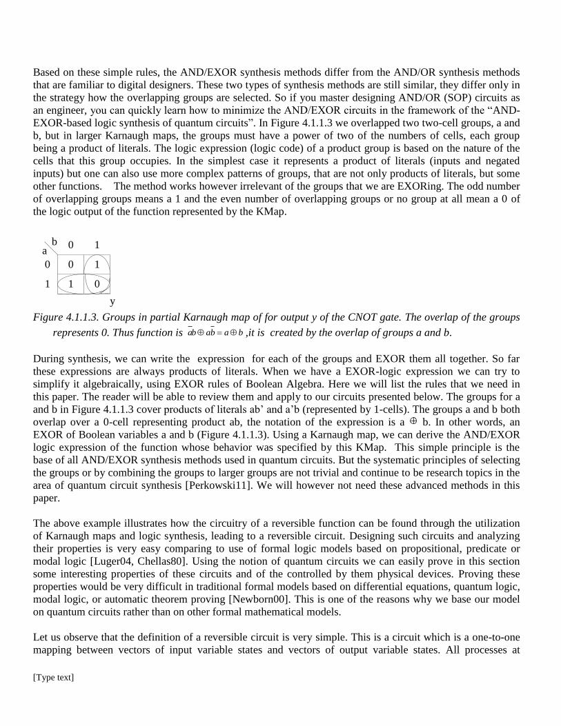
Based on these simple rules, the AND/EXOR synthesis methods differ from the AND/OR synthesis methods
that are familiar to digital designers. These two types of synthesis methods are still similar, they differ only in
the strategy how the overlapping groups are selected. So if you master designing AND/OR (SOP) circuits as
an engineer, you can quickly learn how to minimize the AND/EXOR circuits in the framework of the “AND-
EXOR-based logic synthesis of quantum circuits”. In Figure 4.1.1.3 we overlapped two two-cell groups, a and
b, but in larger Karnaugh maps, the groups must have a power of two of the numbers of cells, each group
being a product of literals. The logic expression (logic code) of a product group is based on the nature of the
cells that this group occupies. In the simplest case it represents a product of literals (inputs and negated
inputs) but one can also use more complex patterns of groups, that are not only products of literals, but some
other functions. The method works however irrelevant of the groups that we are EXORing. The odd number
of overlapping groups means a 1 and the even number of overlapping groups or no group at all mean a 0 of
the logic output of the function represented by the KMap.
a
0
1
0
0 1
1
b
1
1 0
y
Figure 4.1.1.3. Groups in partial Karnaugh map of for output y of the CNOT gate. The overlap of the groups
represents 0. Thus function is bababa ,it is created by the overlap of groups a and b.
During synthesis, we can write the expression for each of the groups and EXOR them all together. So far
these expressions are always products of literals. When we have a EXOR-logic expression we can try to
simplify it algebraically, using EXOR rules of Boolean Algebra. Here we will list the rules that we need in
this paper. The reader will be able to review them and apply to our circuits presented below. The groups for a
and b in Figure 4.1.1.3 cover products of literals ab’ and a’b (represented by 1-cells). The groups a and b both
overlap over a 0-cell representing product ab, the notation of the expression is a b. In other words, an
EXOR of Boolean variables a and b (Figure 4.1.1.3). Using a Karnaugh map, we can derive the AND/EXOR
logic expression of the function whose behavior was specified by this KMap. This simple principle is the
base of all AND/EXOR synthesis methods used in quantum circuits. But the systematic principles of selecting
the groups or by combining the groups to larger groups are not trivial and continue to be research topics in the
area of quantum circuit synthesis [Perkowski11]. We will however not need these advanced methods in this
paper.
The above example illustrates how the circuitry of a reversible function can be found through the utilization
of Karnaugh maps and logic synthesis, leading to a reversible circuit. Designing such circuits and analyzing
their properties is very easy comparing to use of formal logic models based on propositional, predicate or
modal logic [Luger04, Chellas80]. Using the notion of quantum circuits we can easily prove in this section
some interesting properties of these circuits and of the controlled by them physical devices. Proving these
properties would be very difficult in traditional formal models based on differential equations, quantum logic,
modal logic, or automatic theorem proving [Newborn00]. This is one of the reasons why we base our model
on quantum circuits rather than on other formal mathematical models.
Let us observe that the definition of a reversible circuit is very simple. This is a circuit which is a one-to-one
mapping between vectors of input variable states and vectors of output variable states. All processes at
[Type text]
quantum level other than measurement are reversible. Reversibility can be easily checked for the Feynman
Gate from Figure 4.1.1.1. The Feynman gate is thus a reversible gate, and also a reversible circuit. Every
circuit composed from the reversible gates can be also implemented (built) in quantum technologies, we call it
the quantum circuit. There are other types of quantum circuits which we will discuss later on, but now we will
concentrate on these quantum circuits that are reversible and use binary logic with values zero and one for
signals. We call them reversible binary quantum circuits or permutative quantum circuits (for reasons
explained below).
For any single output Boolean function, we can write the Karnaugh map based on how the desired function
transforms input vectors to the output value. Similarly a function with many outputs can be described by m
KMaps or by a single KMap with binary strings of length m in each cell. It is often more convenient to create
directly a KMap from the natural language specification of the problem rather than to first create a truth table
and next convert it to a KMap. Similarly as we have done above, from the KMap, the designer can find
groups and use various logic synthesis procedures to simplify the function into a collection of basic functions
(OR, AND, EXOR). Therefore, the designer can derive the circuitry of the desired function specification. This
is very similar to the ways how the traditional computers are designed. The circuit with AND, OR and EXOR
elements can be next converted to a reversible circuit, possible with some wires (inputs to the circuit)
initialized to logic constants. The wires (bits) of the circuit that are initialized to constant values 0 or 1 are
called the ancilla bits. Another method is to directly use reversible gates in the synthesis, which will be
discussed in the sequel. Although KMap is useful to invent new methods, it is only a means to design an
efficient computer algorithm that executes the entire synthesis.
As we will illustrate in the next section, Kmaps are also useful for truly quantum (non-permutative) circuit
synthesis. We call them the Quantum QMaps. When a function is reversible, the Quantum Map and the
Karnaugh Map are exactly the same.
4.2. From reversible gates to quantum gates.
4.2.1. Quantum Superposition and its visualization in Kmap.
In quantum computers, one is allowed to use only quantum states instead of the classical states. So, the spin of
an electron or a polarization of a photon can be replaced by some abstract “quantum state”: the quantum bit
(qubit for short). Just as a bit has a state 0 or 1, a qubit also has a state 0 or 1 . Symbols 0 and 1 are called
kets in Dirac Notation. The difference between bits and qubits is that a qubit can also be in a linear
combination of states 0 and 1 :
10
The Dirac notation which is a standard notation for states in Quantum Mechanics and we say that kets 0 and
1 are in a superposition.
Definition 2.1.
The state is called a superposition of the states and with
amplitudes α and β (α and β are complex numbers).

[Type text]
Thus, the state is a vector in a two-dimensional complex vector space with basis vectors 0 and 1 . The
matrix (Heisenberg notation) representations of the vectors 0 and 1 are given by
1
0
for State 0 ,
0
1
for State 1 . Thus =
0
+
0
=
is a vector of complex
amplitudes.
Quantum mechanics tells us that if one measures the state |γ> one gets either 0 , with probability αα* ( |α|2) ,
or 1 with probability (|β|2). Here, α* is the complex conjugate of α. If α was a complex number g + bi,
the conjugate would be g – bi (i2 = -1). That is, measurement changes the state of a qubit. In fact, any attempt
to find out the amplitudes of the state |γ> produces a nondeterministic collapse of the superposition to either
0 or 1 basis states (eigenvectors). If | α |2
and | β |2
are probabilities and there are only two possible outputs,
then the calculation as in Figure 4.2.1.1 can be done. This is amazing, isn’t it? Nobody understands why this
mathematics applies to the quantum world and what is the deep meaning of quantum phenomena. Richard
Feynman, Nobel Prize Laureate in Physics said: “I think I can safely say that nobody understands Quantum
Mechanics”12. However, many experiments proved that this is how our Universe works. When we say
Quantum Mechanics we mean the postulates, the Hilbert space and the formalisms as the above. It is the
mathematical apparatus that has been confirmed by experiments multiple times, not the interpretation of QM.
Amazingly, many philosophical interpretations of QM are possible for the same formalism. What the
physicists understand is not the concept of quantum mechanics but its mathematics. In this section, we follow
the same steps: we accept the axioms, we derive the consequences, we do not understand the essence, we
assume one interpretation – Copenhagen.
We will discuss more on quantum mechanics in the next sub-sections, but now let us keep focused on the
mathematics of quantum circuits as we will have to use it soon in practical applications of robot models built
to visualize our philosophical arguments.
Sum of all event’s probabilities is “1” so that
| α |2 + | β |
2 = 1
12 http://www.spaceandmotion.com/quantum-mechanics-richard-feynman-quotes.htm

[Type text]
1
0
10
12
10
2
1
2
2
StateBasic
StateSuperposed
Figure 4.2.1.1: Explanation of superposed states and their measurements.
4.2.2. Calculating a quantum state using matrices.
Any quantum circuit, both small and very large, such as a quantum computer, can be represented by a unitary
matrix. M is a unitary matrix when M+
* M = M * M+
= I, where I is an identity matrix, and M+ is a hermitian
adjoint matrix of M, it means conjugate transpose matrix ( * is standard matrix multiplication).
The state of the quantum circuit (input state, internal state after any gate, or output state) is represented by a
vector of complex numbers. The unitary matrix of the circuit, when multiplied by the input state vector,
creates the output state vector. It is important to appreciate that this representation, the unitary matrix, remains
the same for any size of the circuit. The smallest matrices represent single rotations of electrons or other
particles, examples of them are Pauli rotations [Nielsen00]. Big matrices describe a complete quantum
algorithm, such as the (quantum) Grover algorithm [Nielsen00], which can solve difficult problems much
faster than any existing computer on the Earth, provided that it has a sufficient number of qubits. The circuit
is an operator acting on the state vector. We can talk about the matrix of the operator, but we will use names
“operator”, “circuit”, “gate” and “unitary matrix” interchangeably.
A simple example of generating an output quantum state from the input state vector and the matrix of operator
acting on the input state is shown in Heisenberg notation and next in Dirac notation in Figure 4.2.1.2.
Heisenberg notation uses matrices and Dirac notation uses expressions with kets |0 and |1.
H * |0 =
1
2
1 1
1 1
1
0
1
2
1
1
1
20
1
21
Figure 4.2.1.2.: Matrix representation of state 0 going through Hadamard gate H. Heisenberg notation uses
matrices to describe operators and vectors for states. The Dirac notation is presented at the right. Here |0
and |1 are called “kets”.
In Figure 4.2.1.2 one can see how an input state reacts to the gate represented as a unitary matrix. What is
shown is the input vector, state |0, is acted upon by the Hadamard gate (Hadamard operator). When a circuit
(Operator, Matrix) acts upon an input vector, it is simply multiplied by the matrix of the circuit, following the
[Type text]
rules of standard matrix multiplication. The Dirac notation at the right of Figure 4.2.1.2 is more convenient
for some symbolic calculations and interpretation. We will be therefore using both Heisenberg and Dirac
notations in this paper. We see from Figure 4.2.1.2 that the probability of measuring state |0 is ½ and that the
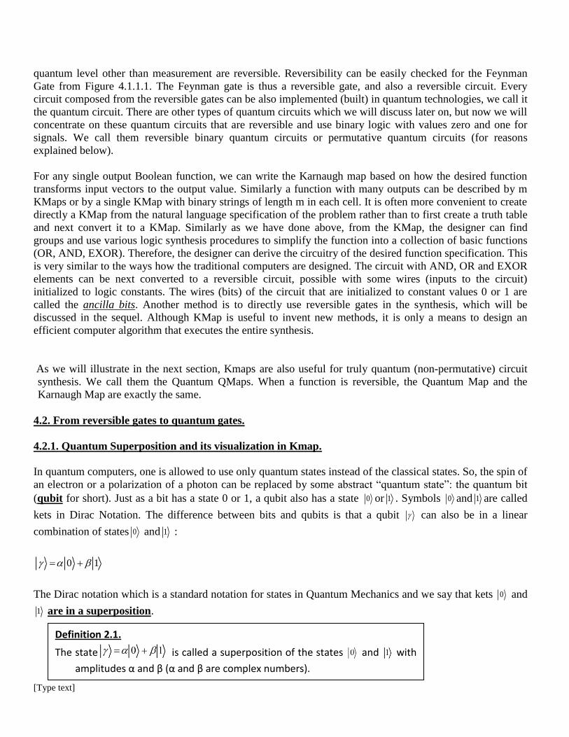
probability of measuring state |1 is also ½. If |0 represents “dead” and |1 represents “alive” the qubit from
Figure 4.2.1.2. represents the quantum state “half dead and half-alive”, which is known as the property of the
famous Schroedinger Cat and is also called the “cat state” [Nielsen00].
4.2.2.1. Calculating the Kronecker Product on matrices.
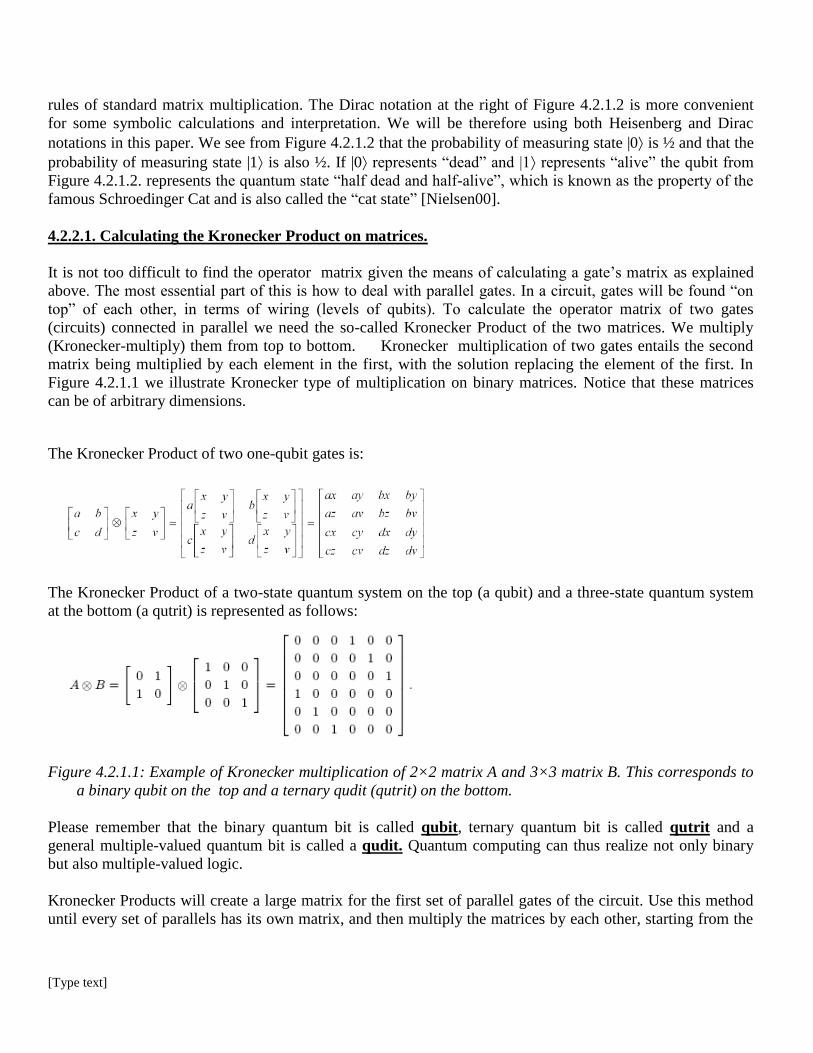
It is not too difficult to find the operator matrix given the means of calculating a gate’s matrix as explained
above. The most essential part of this is how to deal with parallel gates. In a circuit, gates will be found “on
top” of each other, in terms of wiring (levels of qubits). To calculate the operator matrix of two gates
(circuits) connected in parallel we need the so-called Kronecker Product of the two matrices. We multiply
(Kronecker-multiply) them from top to bottom. Kronecker multiplication of two gates entails the second
matrix being multiplied by each element in the first, with the solution replacing the element of the first. In
Figure 4.2.1.1 we illustrate Kronecker type of multiplication on binary matrices. Notice that these matrices
can be of arbitrary dimensions.
The Kronecker Product of two one-qubit gates is:
The Kronecker Product of a two-state quantum system on the top (a qubit) and a three-state quantum system
at the bottom (a qutrit) is represented as follows:
Figure 4.2.1.1: Example of Kronecker multiplication of 2×2 matrix A and 3×3 matrix B. This corresponds to
a binary qubit on the top and a ternary qudit (qutrit) on the bottom.
Please remember that the binary quantum bit is called qubit, ternary quantum bit is called qutrit and a
general multiple-valued quantum bit is called a qudit. Quantum computing can thus realize not only binary
but also multiple-valued logic.
Kronecker Products will create a large matrix for the first set of parallel gates of the circuit. Use this method
until every set of parallels has its own matrix, and then multiply the matrices by each other, starting from the

[Type text]
rightmost column towards the leftmost. Once this is done, the operation matrix of the entire circuit will is
found.
2.3. Quantum states calculated by the Hadamard gate
In this subsection we will introduce the Hadamard gate. A quantum Hadamard Transform for two qubits can
be done just by placing such gates in parallel (Figure 4.3.3) in the quantum array. A Hadamard Transform is
known from classical binary circuits, and has applications in signal processing. It is a complex circuit in
binary logic with many adders and subtractors connected by complex “butterfly” network of connections. But
Hadamard Transform for any number of qubits becomes a very inexpensive and small circuit in quantum –
just put the Hadamard gates in parallel! Hadamard Transform on many qubits is just one way to illustrate the
power of quantum computing. The Hadamard gate is represented by a 2-by-2 matrix from Figure 4.3.1.
Applying the gate to states 0 and 1 we obtain states that in Dirac notation are shown in Figure 4.3.2. The
careful reader can wonder how we can draw the superposed states created by this gate in a quantum Kmap.
We will come back to this question soon.
1 1
1 -1 1
2
Figure 4.3.1: The Hadamard gate matrix.
Figure 4.3.2 :Dirac notation of Hadamard outputs.
The Hadamard gate followed directly be the quantum measurement gate acts like an ideal random number
generator, with one input and one output. When the Hadamard gate operates on inputs 1 or 0 , the resulting
outputs after measurement will be identical. Though the result for 1 has a - 1 entry instead of 1 , this is
irrelevant in measurement since all probability amplitudes are squared if the output of H is directly measured
(i.e., the global quantum phase is lost). The output state before the measurement (see Figure 4.3.2) represents
an equal probability of states 1 and 0 , but it represents also the phase. As the coefficient becomes the
amplitude of both states, the square of it (1/2) becomes the probability of that state if this state is measured. In
case of the measurement the phase is not relevant at all! However, before the measurement few next quantum
operators can be executed on this state, so the phase of this state is relevant in such a case. This property of
quantum states is very important. It is used for instance in the famous quantum Grover algorithm to solve very
many combinatorial problems faster than on a normal computer [Nielsen00].
The KMap of the Hadamard gate is shown in Figure 4.3.5. It is called Quantum Map or a QMap, because
Hadamard gate, as you see in its unitary matrix, is not a permutative gate, since the unitary matrix is not a
permutative matrix. The QMap of the gate gives the complete information about the output quantum states for
all possible input basis states.

[Type text]
In Figure 4.3.3 a Superposition state created by the Hadamard gate is shown. Figure 4.3.4 repeats these
calculations using the Heisenberg notation. As often done by physicists, the coefficient 2
1 is omitted in this
particular calculation.
Figure 4.3.3: The symbolic notation for a Hadamard gate that is controlled by various basis states.
Figure 4.3.4: Analysis of Hadamard gate applied to various input states.
Figure 4.3.5. illustrates the quantum K-map of the Hadamard gate.
0 0.7071 0
+0.7071 1
1 0.7071 0
-0.7071 1
Figure 4.3.5: The Quantum Kmap of the output of Hadamard gate (from Matlab software).
10
0
10 toapply Hadamard
1
01 toapply Hadamard
101
1
0
1
11
11
101
1
1
0
11
11

[Type text]
Figure 4.3.6: The EPR circuit that illustrates the concept of entanglement.
Now we will explain the basic resource of quantum computing, the phenomenon that exists only in quantum
mechanics and that is responsible for difference of quantum mechanics and classical computing. We will do
this using the famous EPR circuit which illustrates the “thought experiment” published by Einstein, Podolsky
and Rosen [Einstein35, Nielsen00]. This circuit is given in Figure 4.3.6. and its corresponding quantum K-
map in Figure 4.3.7. The quantum state in this table (QMap) have been verified using Matlab as in Figure
4.3.16.
P, Q
Figure 4.3.7. The quantum KMap illustrating the output state of the EPR circuit. This KMap visualizes the
entanglement from the circuit in Figure 4.3.6.
b
a
0 1
0 0.7071 00
0 01
0 10
0.7071 11
0 00
0.7071 01
0.7071 10
0 11
1 0.7071 00
0 01
0 10
-0.7071 11
0 11
0.7071 01
-0.7071 10
0 11
Figure 4.3.8: Matlab simulation to find the Quantum KMap for EPR circuit.
We will analyze the EPR circuit next and we will discuss its importance.
4.4. Visualization of quantum states in larger gates.
b
a
0 1
0 112
100
2
1 10
2
101
2
1
1 102
101
2
1 11
2
100
2
1

[Type text]
4.4.1. The Feynman or CNOT gate
For illustration we will compare various notations for the same gate. This is the CNOT gate from Figure 4.3.6
used in EPR circuit above. Its permutative matrix is 4-by-4, as shown in Figure 4.2.2.1a and its KMap is
shown in Figure 4.2.2.1b. Please compare the matrix and the KMap.
1 0 0 0
0 1 0 0
0 0 0 1
0 0 1 0
ab
1
0
0
0,1
1,0
P,Q
0,0
1
1,1
c
a) b) c)
Figure 4.4.1: (a) Feynman gate, (b) Feynman gate matrix, (c) the KMap of the Feynman gate.
Many of CNOT gate properties have been already discussed here, but more will come. It is basically a
reversible EXOR gate, reversible in that each qubit is continued to an output, unlike the classical EXOR. It is
also deterministic, unlike the Hadamard, which means that a given input vector will always register the same
output value. This gate is inexpensive in quantum and thus should be made the base of the synthesis. This
gate is linear and thus it is not universal (linear gate realizes a linear function. Linear function can be
expressed using EXOR operators only on input variables). To make a universal system we will need one more
gate – the Toffoli gate. In theory, every quantum computer can be built using only CNOT and Hadamard
gates, but like nobody builds standard computers from (universal) gates NAND, so in the quantum technology
world we use non-minimal sets of gates to build quantum computers.
4.4.2. The 3*3 Toffoli or CCNOT gate
The Toffoli gate is an interesting and powerful gate in that it can have any number of inputs and the EXOR can
be located in any wire of it. To be of practical usage, it must take these many forms. The circuitry is as in
Figure 4.4.2.1:
a
b
c
p
q
r
p, q, r
c
ab
0 1
00 000 001
01 010 011
11 110 110
10 100 101
Changes are only when a = b =
1

[Type text]
P = a, Q = (b c) (ab c ) = b ca
R = a.(b c) c = ab c
Figure 4.4.2.1: The 3*3 Toffoli gate. It is also called the Controlled-Controlled-NOT or the CCNOT gate. The
right part of the figure shows the Kmap for this gate.
We can see that it is a double controlled inverter. One might think that the addition of another control would
still make it a close relative of the Feynman. That is not so. For the Toffoli has 3 inputs, a, b, and c, and the
designer can put constants in any of those positions, thus transforming the gate. By manipulations of this
property, one can derive classical gates, and thus, prove that the Toffoli is a universal quantum gate.
The input/output relationship is p = a , q = b and r = ab c. Although Toffoli is a generalized form of the
Feynman gate, the Toffoli gate is a universal gate in both classical and reversible (but not quantum) logic but
the Feynman gate is not universal. On the other hand Feynman gate is linear gate but Toffoli gate is not.
These gates are then complementary and using them together leads to a synergy. With Inverter, Feynman,
Hadamard and Toffoli we can create an arbitrary quantum circuit, but we will introduce more quantum gates
for didactic reasons.
4.4.3. The 3 * 3 Fredkin or Controlled-SWAP gate
Figure 4.5.1: Fredkin gate realized using Toffoli and CNOT gates. At right we illustrate algebraic analysis
method using Boolean and EXOR algebra. As this gate has 3 inputs and 3 outputs we will call it a 3*3 gate.
Fredkin gate in quantum array form is analyzed as in Figure 4.5.1.
4.6. The Ancilla qubits
Ancilla qubits are extra qubits. They are not variables, though they can be mapped onto an output. Ancilla
qubits are useful for input variables in 3*3 and larger gates, as well as on wires that lead to the output. In a
large circuit, it is not always good to have every wire assigned to a variable input; the functions of the gates
can be changed in useful ways if some of the wires are assigned to a constant. One has to add ancilla bits
when an arbitrary Boolean function is converted to a reversible circuit.
To explain ancilla uses in large gates, one must look no further than the Toffoli gate. In order for the Toffoli
to be of use, in many cases the wire that goes to the EXOR must have a constant value (1 or 0) to change its
uses and allow it to be a universal gate. Those 1’s and 0’s are ancilla bits, since they are not input variables,
and are constant. They can also be placed on wires leading to an output, whether it is because the ancilla bit
was on the answer register of the final gate, or because it is simply more efficient to do so. Figure 4.6.1
illustrates how AND and NAND gates of classical logic can be built using the Toffoli gate with the lowest

[Type text]
qubit being an ancilla bit. As we see in the example, ancilla bit is absolutely necessary if we want to convert a
non-reversible function (called also an irreversible function) like AND or EXOR into reversible (quantum)
circuit.
(a) AND (b) NAND
Figure 4.6.1: (a) Realization of AND gate using Toffoli gate with the ancilla qubit initialized to zero, (b)
Realization of NAND gate using Toffoli gate with the ancilla qubit initialized to one.
Dear reader, if you are tired of all these quantum formalisms, feel free to relax now. We are done with basic
quantum circuit material and in theory you have enough knowledge to create your own models of quantum
circuits, quantum automata, quantum games, quantum computers or “quantum brains” of robots. Then, if you
assume randomness in measurements you will be fully on the ground of QM, if you assume that sometimes or
always some outside mechanism (God) influences measurements, you are on the ground of our model. The
interpretation of quantum measurement is the only difference of our approach from the accepted model used
in quantum computing.
4.7. Quantum Braitenberg Vehicles
Figure 2.7.1. The simplest Breitenberg Vehicles with analog control, (a) each sensor is connected to the motor on the same side, (b) each sensor connected to the motor on opposite side, (c) both sensors connected to both the motors.
Figure 2.7.2. The vehicle at left avoids light while the vehicle at right follows light.

[Type text]
4.7.1. Classical Braitenberg Vehicles
Valentino Braitenberg wrote a revolutionary book titled Vehicles: Experiments in Synthetic Psychology
(Publisher: Cambridge, Mass. MIT Press, 1986), [Braitenberg86] . This book influenced modern robotics
more than any other book written by a psychologist. In the book Braitenberg describes a series of thought
experiments. It is shown in these experiments that simple systems (the vehicles) can display complex life-like
behaviors far beyond those which would be expected from the simple structure of their “brains.” He describes
a law termed the “law of uphill analysis and downhill invention”. This law explains that it is far easier to
create machines that exhibit complex behavior than it is to try to build the structures from behavioral
observations. By connecting simple motors to sensors, crossing wires, and making some of them inhibitory,
we can construct simple robots that can demonstrate behaviors similar to fear, aggression, affection, and
others. The original vehicles use only analog signals or Boolean Logic in their controlling circuits, but we
generalized these ideas to multiple-valued, fuzzy, probabilistic, and quantum logics and we designed
“emotional robots” that combine various types of logic – a task which is easy when all control is simulated in
software [Perkowski11]. The concept of Quantum Braitenberg Vehicles (QBV) was introduced in
[Raghuvanshi07].
The first vehicle (Figure 4.7.1) has two sensors and two motors, at the right and left. The vehicle can be
controlled by the way the sensors are connected to the motors. Braitenberg defines three basic ways we could
possibly connect the two sensors to the two motors.
(a) Each sensor is connected to the motor on the same side.
(b) Each sensor is connected to the motor on the opposite side.
(c) Both sensors are connected to both motors.
Type (a) vehicle will spend more time in places where there are less of the stimuli that excite its sensors and
will speed up when it is exposed to higher concentrations. If the source of light (for light sensors) is directly
ahead, the vehicle may hit the source unless it is deflected from its course. If the source is to one side, then
the sensor nearer to the source is excited more than the other and the corresponding motor turns faster. As a
consequence, the vehicle will turn away from the source. Turning away from the source (a shy behavior) is
illustrated at left in Figure 4.7.2.
We can observe another type of vehicle, type (b), with a positive motor connection. There is no change if the
light source is straight ahead, a similar reaction as seen in type (a). If it is to either side, then we observe a
shift in the robot’s course. Here, the vehicle will turn towards the source and eventually hit it. As long as the
vehicle stays in the vicinity of the source, no matter how it stumbles and hesitates, it will eventually hit the
source frontally. If the two vehicles are let loose in an environment with sufficient stimuli, their characters
emerge. The type (a) vehicle with a positive connection will become restless in its vicinity and tend to avoid
stimuli until it reaches a place where the influence of any light sources is scarcely felt. This vehicle exhibits
fear. A vehicle of type (b) with a positive connection turns toward the source of light and impacts with it at a
high velocity. The aggressive behavior is displayed clearly.
Next, Braitenberg presented thought experiments with increasingly complex vehicles built from the standard
mechanical and electrical components of his time. Braitenberg’s goal was to explore the nature of
intelligence and psychological ideas that were not related to quantum control. Even so, more and more

[Type text]
intricate behaviors emerge from creating various interactions between components; see [Braitenberg86] The
“vehicles” that we worked on are not merely mobile wheeled robots like those from [Braitenberg86], but
humanoid bipeds, human and animal torsos with heads, so that we can create much more interesting and
sophisticated movements, although the general principle of behavioral robotics as illustrated in Braitenberg
Vehicles (the evolution of complex behaviors from simple descriptions) remains. Multiple-valued quantum
automata hold many advantages over simple binary combinational circuits.
4.7.3. Practical use of quantum formalisms in robot control design.
A quantum gate in series with another quantum gate will retain the dimensions of the quantum logic system.
The resultant matrix is calculated by multiplying the operator matrices in a reverse order (standard matrix
multiplication). With this background, a teenage Lego robot builder can construct and analyze quite complex
robot controllers with deterministic behaviors (they have permutative unitary matrices). Now the students
raise a question – “where is the quantumness?” and the time comes to introduce the notation and the unitary
matrix of a very important quantum gate – the Hadamard gate (Fig. 4.3.1). This is a “truly quantum” gate that
cannot be realized in a binary or permutative reversible circuit. This is in contrast to permutative gates
(described by permutative matrices) that can be realized by standard reversible logic circuits.
Connecting two Hadamard gates in series we obtain the input signal back – so they work together as a wire
(identity). However, measuring the intermediate signal would give ½ probability of |0 and ½ probability of
|1.
The quantum circuit from Fig. 4.7.4.9 can be split into 3 circuits as shown below. Here, the Hadamard gate
(gate Y in Figure 4.7.10) is connected in parallel to a wire (gate Z in Figure 4.7.4.10). Next, the parallel
connection of gates Y and Z is in a series with the Feynman gate (gate X in Figure 4.7.4.12). We need the
Kronecker Product to calculate the parallel connection and standard matrix multiplication to calculate the
serial connection. This is shown step-by-step in Figures 4.7.4.9 through 4.7.4.13.
Fig. 2.7.4.10. Calculation of parallel connection of gates H and wire
Fig. 2.7.4.9. The quantum controller for the EPR robot. This circuit produces entanglement that can be analyzed by robot behaviors
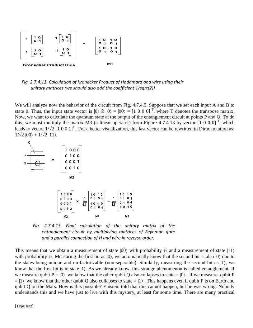
[Type text]
We will analyze now the behavior of the circuit from Fig. 4.7.4.9. Suppose that we set each input A and B to
state 0. Thus, the input state vector is |0 |0 = |00 = [1 0 0 0] T
, where T denotes the transpose matrix.
Now, we want to calculate the quantum state at the output of the entanglement circuit at points P and Q. To do
this, we must multiply the matrix M3 (a linear operator) from Figure 4.7.4.13 by vector [1 0 0 0] T
, which
leads to vector 1/2 [1 0 0 1]T
. For a better visualization, this last vector can be rewritten in Dirac notation as:
1/2 |00 + 1/2 |11.
This means that we obtain a measurement of state |00 with probability ½ and a measurement of state |11
with probability ½. Measuring the first bit as |0, we automatically know that the second bit is also |0 due to
the states being unique and un-factorizable (non-separable). Similarly, measuring the second bit as |1, we
know that the first bit is in state |1. As we already know, this strange phenomenon is called entanglement. If
we measure qubit P = |0 we know that the other qubit Q also collapses to state = |0 . If we measure qubit P
= |1 we know that the other qubit Q also collapses to state = |1 . This happens even if qubit P is on Earth and
qubit Q on the Mars. How is this possible? Einstein told that this cannot happen, but he was wrong. Nobody
understands this and we have just to live with this mystery, at least for some time. There are many practical
Fig. 2.7.4.11. Calculation of Kronecker Product of Hadamard and wire using their unitary matrices (we should also add the coefficient 1/sqrt(2))
Fig. 2.7.4.13. Final calculation of the unitary matrix of the entanglement circuit by multiplying matrices of Feynman gate and a parallel connection of H and wire in reverse order.

[Type text]
and philosophical applications of this phenomenon. For instance, it illustrates non-locality of quantum
mechanics: one particle on Earth, one on the end of Galaxy, entangled, know mutually their quantum states
and lead to measurements |00 or |11.
Assume now that signals A and B come from sensors S1 and S2 as in Fig. 4.7.4.1a, and P and Q go to motors
M1 and M2. Assume also that 0 signifies no light to the sensor and 1 is light, and that 0 is no motor
movement while 1 is full speed forward movement. If there is no light in front of the robot, the robot will
randomly either stay stable (both motors have 0) or will move forward (both motors will have 1). The
combinations 01 and 10 for the motors are not possible because their corresponding eigen-states have null
amplitudes. The robot cannot thus turn right or left in this situation. It is left to the students to analyze
behaviors of this robot for every possible binary input combination. Next the students can analyze what will
happen if gate H is removed from the controller. Can the robot turn left and right? Does there exists an
entanglement between states |01 and |10, which would mean that the robot would never stop or go straight
but keep turning left and right randomly? When? This is the kind of challenge questions asked the students.
Observe that if we had two H gates in parallel as the controller and there were no light present, then every
combination of motors 00 (stop), 01 (turn left), 10 (turn right), and 11 (go forward) would be possible with
equal probability. When measured, the Hadamard gate works as ideal random number generator. It can be
controlled by an arbitrary quantum signal that allows us to control the probabilistic and entangled behaviors of
the robot. Suppose that the Hadamard gate in Fig. 4.7.4.9 is controlled by one more wire D. If D = 0, the
circuit is just a Feynman gate, which means that when both sensor inputs A and B are 1, signal P is 1 but
signal Q is 0 (since 11 = 0) and the vehicle will turn right. Similarly, we can find deterministic behaviors of
the vehicle for any input combination. However, when D = 1, the Hadamard gate starts to operate and the
circuit works as the explained earlier entanglement circuit.
As we discussed at the beginning of this section of the paper, every combinational circuit (non-reversible) can
be transformed into a reversible (permutative quantum) circuit by adding so-called ancilla bits (constants to
inputs and garbage bits to outputs). In this way, we can transform every standard automaton (Finite State
Machine with binary flip-flops) to a (binary) quantum automaton. Because the Hadamard gate works as an
ideal random number generator, with equal probabilities of signals 0 and 1 at its output, every probability with
accuracy to 1/2N
can be generated with N controlled Hadamard gates.
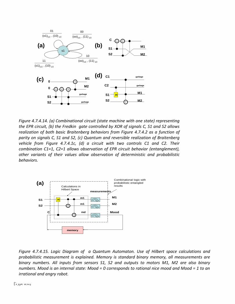
[Type text]
s1
00
(oo)1/2 , (11) 1/2
01
(o1)1/2 , (10) 1/2
11
(o1)1/2 , (10) 1/2
10
(oo)1/2 , (11) 1/2
(a) (b)
(c)(d)
C
S1
S2 M2
M1
C2
S1
S2 M2
M1
0
S1
S2
garbage
garbage
0M1
M2
H
C1 garbage
garbage
(a)
C
S1
S2M2
M1H
Mood
Combinational logic with
probabilistic entangled
results
memory
m1
m1
md
Calculations in
Hilbert Spacemeasurements
Figure 4.7.4.14. (a) Combinational circuit (state machine with one state) representing the EPR circuit, (b) the Fredkin gate controlled by XOR of signals C, S1 and S2 allows realization of both basic Braitenberg behaviors from Figure 4.7.4.2 as a function of parity on signals C, S1 and S2, (c) Quantum and reversible realization of Braitenberg vehicle from Figure 4.7.4.1c, (d) a circuit with two controls C1 and C2. Their combination C1=1, C2=1 allows observation of EPR circuit behavior (entanglement), other variants of their values allow observation of deterministic and probabilistic behaviors.
Figure 4.7.4.15. Logic Diagram of a Quantum Automaton. Use of Hilbert space calculations and probabilistic measurement is explained. Memory is standard binary memory, all measurements are binary numbers. All inputs from sensors S1, S2 and outputs to motors M1, M2 are also binary numbers. Mood is an internal state: Mood = 0 corresponds to rational nice mood and Mood = 1 to an irrational and angry robot.
[Type text]
This allows realization of an arbitrary probabilistic automaton in quantum (at the price of adding the ancilla
bits). The deterministic automaton is a special case of a probabilistic automaton (a probabilistic automaton
can be described by a probabilistic matrix, and a deterministic automaton by a permutative matrix). Finally,
the quantum circuit (like our entanglement circuit) can be represented by a unitary matrix with complex
numbers for transitions. Therefore, the quantum automaton is the most powerful theoretical concept of
computing that is physically realizable at the time of this writing. It includes the combinational and
probabilistic functions and automata as well as quantum combinational functions (quantum circuits) as its
special cases. There is no doubt that the Quantum Automaton Robot is much more powerful than a
Braitenberg Vehicle, which fact we have observed by constructing and simulating quantum equivalents of the
known Braitenberg Vehicles. A simple Quantum Automaton Robot controller is shown in Fig. 4.7.4.15. This
controller can be used with similar but not exactly the same effects in several robots. Observe entanglement
for S1 = 0, S2 = 0, C = 1.
Concluding this section let us stress that the model outlined in this section is not a metaphysical model from
sections 1 - 3, but a purely physical model that completely agrees with Copenhagen interpretation of QM.
Next section will create a circuit model based on the metaphysical model, combining thus the two above
models to allow visualization and modeling, as well as computerization.
5. Modeling in the MQMM model
5.1. Simple Practical Example of modeling in MMQM model
In section 4 we used mathematical apparatus of quantum circuits (quantum computing) to explain
fundamental ideas of designing simple practical quantum circuits and quantum robots. The six axioms of QM
were the base of this apparatus. We were operating entirely in the domain of physics and engineering, without
any metaphysical assumptions.
Now we will assume however that in addition to the six axioms we use also AXIOM 8 from Section 3.
Example 5.1.
Let us now discuss QBV EPR as the simplest possible model in our FAS system MMQM. Suppose that we
have a QBV EPR vehicle that because of an entanglement in its controller creates the quantum state
112
100
2
1 . It means that with probability ½ the robot stops and with probability ½ the robot drives some
distance forward (say 2 cm). Let us assume that this vehicle is physically realized as a robot and AXIOM 8 is
now allowed to operate.
Question.
What is the God’s potential for QBV EPR according to standard QM theory from Section 4 assuming
Copenhagen Interpretation?
Answer.
For QBV EPR God can only select between measuring |00 and |11. God cannot cause measurements |01 or
|10. Selecting however subsequently many times between |00 and |11 God can select the speed of motion,
regularity of motion and in extreme cases God can stop the robot entirely, or make it move forward with the

[Type text]
highest speed. But God cannot make this vehicle turn right or turn left. This is a consequence of our axiomatic
assumption – God following the rules of the created by Him system (God cannot violate its own rules).
This example leads us to the problem of correct understanding what is God’s Omnipotence.
5.2. God’s Omnipotence in the MMQM model
We used above the words that “God in our model “cannot do” certain changes to the physical world”. God is
from definition Omnipotent, thus “God can do everything”, but God cannot contradict logic 13. Obviously, as
we distinguish a formal system within our model, violating any of its axioms would “imply contradiction”.
Making square circles, making 2+2 = 5, or violating axioms of Boolean algebra or quantum postulates is
inconsistent with the creation of these laws by God. God just cannot violate quantum postulates if QM is
correct, the same way as God cannot violate the arithmetic fact that 2+2=4. In our Universe, God cannot
violate the fact 2+2=4 even once! God can create another standard arithmetic for another Universe but not in
this Universe.
1. Note, that if a physicist would build the above QBV EPR robot as a real robot and would see that the robot
permanently does not move, he would think that some error was done in the assembly of the robot. If the
robot would move full speed the physicist would also think that an error was done in calculations or
construction. Both these robot behaviors are of extremely low probability using QM measurement axiom
statistically.
2. These “low probability behaviors” can occur as “miracles” that God can perform in the maximally
simplified “quantum universes” described by the Braitenberg Vehicles above and their environments.
These miracles are consistent with QM formalism and explainable only in our QM interpretation model.
God can perform such miracles in every system that includes quantum particles, which means practically
for every matter of the Universe.
3. Note that in the above QBV EPR example the probabilities are ½. Instead of ½, the measurement
probabilities can be arbitrarily close to zero or arbitrarily close to 1. Let us assume now that we replace the
robot with a human. Human’s brain and body are a kind of quantum computer MMQM model. As an
answer to certain moral dilemma, a smart and moral human faced with this dilemma creates in his
quantum automaton brain the output states that are deterministic 1 or 0, yes and no, which are his firm
answers to this dilemma. Thus this human gives no freedom to God to influence the randomness of
13 The idea that “God can do everything” is a false understanding of Omnipotence, a problem discussed for instance by
many theologians. God cannot do anything immoral and God cannot cease to exist. Most theistic philosophies do not
claim that God, being Omnipotent, can “do anything”. For instance, in Christian theology God cannot violate His own
rules. In the specific “mini-Universe” of this paper, the rules are the formal rules of QM, also the formal rules of
classical kinematics and control. In general, the rules of matter are part of rules of God (only some of these rules of
matter have been already recognized by humans – these constitute rules of science). The problem “if God can act
against logic?” was discussed by St. Thomas Aquinas [Thomas]. Thomas, in response to questions of a deity performing
impossibilities (such as making square circles), writes that "Nothing which implies contradiction falls under the
omnipotence of God”. There exists a classical problem in theology “can God create a stone that is so heavy that God
cannot raise it?” St. Thomas answer was that this problem formulation is based on a contradiction, the same as in the
case of asking “Can God create a square circle?”
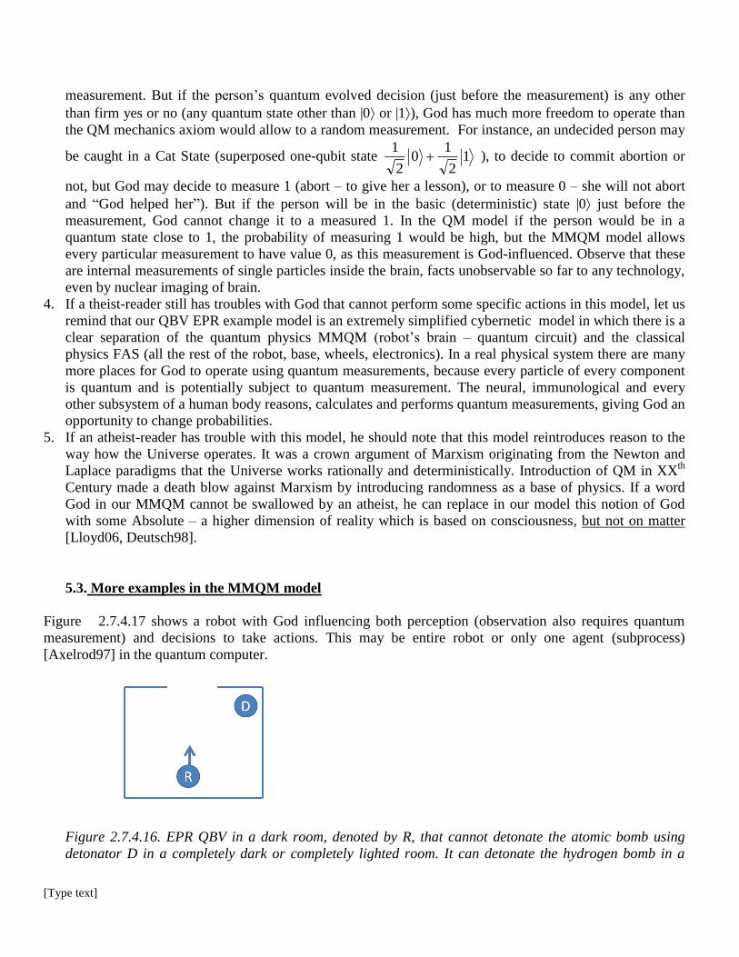
[Type text]
measurement. But if the person’s quantum evolved decision (just before the measurement) is any other
than firm yes or no (any quantum state other than |0 or |1), God has much more freedom to operate than
the QM mechanics axiom would allow to a random measurement. For instance, an undecided person may
be caught in a Cat State (superposed one-qubit state 12
10
2
1 ), to decide to commit abortion or
not, but God may decide to measure 1 (abort – to give her a lesson), or to measure 0 – she will not abort
and “God helped her”). But if the person will be in the basic (deterministic) state |0 just before the
measurement, God cannot change it to a measured 1. In the QM model if the person would be in a
quantum state close to 1, the probability of measuring 1 would be high, but the MMQM model allows
every particular measurement to have value 0, as this measurement is God-influenced. Observe that these
are internal measurements of single particles inside the brain, facts unobservable so far to any technology,
even by nuclear imaging of brain.
4. If a theist-reader still has troubles with God that cannot perform some specific actions in this model, let us
remind that our QBV EPR example model is an extremely simplified cybernetic model in which there is a
clear separation of the quantum physics MMQM (robot’s brain – quantum circuit) and the classical
physics FAS (all the rest of the robot, base, wheels, electronics). In a real physical system there are many
more places for God to operate using quantum measurements, because every particle of every component
is quantum and is potentially subject to quantum measurement. The neural, immunological and every
other subsystem of a human body reasons, calculates and performs quantum measurements, giving God an
opportunity to change probabilities.
5. If an atheist-reader has trouble with this model, he should note that this model reintroduces reason to the
way how the Universe operates. It was a crown argument of Marxism originating from the Newton and
Laplace paradigms that the Universe works rationally and deterministically. Introduction of QM in XXth
Century made a death blow against Marxism by introducing randomness as a base of physics. If a word
God in our MMQM cannot be swallowed by an atheist, he can replace in our model this notion of God
with some Absolute – a higher dimension of reality which is based on consciousness, but not on matter
[Lloyd06, Deutsch98].
5.3. More examples in the MMQM model
Figure 2.7.4.17 shows a robot with God influencing both perception (observation also requires quantum
measurement) and decisions to take actions. This may be entire robot or only one agent (subprocess)
[Axelrod97] in the quantum computer.
Figure 2.7.4.16. EPR QBV in a dark room, denoted by R, that cannot detonate the atomic bomb using
detonator D in a completely dark or completely lighted room. It can detonate the hydrogen bomb in a

[Type text]
partially lighted room (all these assuming no God’s influence on measurement). Even with God’s
influence, if the room is dark the robot cannot detonate the bomb. The arrow shows the initial orientation
of the robot.
Figure 2.7.4.17. A robot with God influencing both perception (observation also requires quantum
measurement) and decisions to take actions.
If the QBV EPR robot MMQM simulation and the above human decision-making speculation based on
MMQM were not dramatic enough, let us visualize to our reader a situation related to free will and
omnipotence in the behavior of future quantum-computer controlled safety robot in a nuclear control room.
Let us assume that the robot R is located in a room (see Figure 2.7.4.16) and that there is a detonator D of an
hydrogen super-bomb.
1. Assume now a new quantum robot with the quantum controller as two individual Hadamard gates for
separate controls of each wheel. One can think about a robot from Figure 2.7.1 with a single Hadamard
gate inserted in left and a single Hadamard gate inserted in right path from sensor to wheel. Putting this
robot to the environment from Figure 2.7.4.16 the hydrogen bomb can be detonated, as random sequences
of control states: (left_wheel, right_wheel) = 00, 01, 10, and 11 will be created. This can be done with no
God’s involvement, assuming only truly random fw-variables of the standard QM interpretation). If God
will be controlling these measurements, He can synchronize left and right wheel by giving only controls
00 and 11 so that the robot will depart from the critical area of the room ( Figure 2.7.4.16).
2. Assuming the quantum controller as QBV EPR circuit and assuming the robot’s environment as a room
with some lights and light sensors of a robot (which would be |11 on EPR robot inputs), the hydrogen
bomb can be detonated (because of Brownian motions resulting from quantum state of wheels control:
102
101
2
1 ).
3. Assuming however the above explained entanglement in QBV EPR and a completely dark room (inputs
|00 of the EPR robot), then God (or Devil, or Guardian Angel, whoever is in control of output
measurement probabilities of this robot) cannot make the robot to approach the detonator and detonate the
hydrogen bomb, because the superposed state would be 112
100
2
1 for which God cannot cause a
single measurement to 01 or 10 which may in turn detonate the bomb.

[Type text]
6. Conclusions
Many examples of thought experiments similar to those presented above can be created and verified on
computer models, but our few examples explain well enough the basic ideas of our model. Some
philosophers argue that QM has to do only with micro-world so it has no relation to humans. This reasoning
is just wrong. As we see from the hydrogen-bomb example in section 5, a single quantum measurement may
hypothetically affect lives of hundreds of thousands of people. The practical and intuitive concepts derived
from Hilbert Space formalisms, such as the quantum circuits, quantum games, quantum automata and
quantum computers are easy to explain; they allow to be better visualized to modern common humans. These
formal concepts are useful especially to engineers who are familiar with circuits, schemata and feedback. The
quantum circuits can be simulated on a normal computer and their behaviors can be visualized and analyzed
statistically. The quantum circuits are what the truly quantum computer does. As people with engineering
minds are familiar with digital circuit schematics, flowcharts and programming, these languages are easier to
communicate theological ideas than the language of mediaeval theology of St. Tomas on one hand, and
modern systems of mathematical logic on the other hand. We believe that these are models and languages
that can be used to better and more precisely communicate theological ideas, but so far these languages are
neglected by philosophers and theologians alike. By doing this, we try to create “a theology for engineers
and programmers”. In contrast to “theology for philosophers” or “theology for masses”, in future, most
people will belong to this category. So our attempt is practical.
We believe that one of applications of our model is early education. By teaching early in life Quantum
Mechanics and interpretations of QM educators can help young people to develop a deeper understanding of
reality. This idea exists in many valuable books by Chopra, Barr, Goswami, Capra, Talbot, etc but these
books use non-scientific terms and try to explain quantum mechanics in lay and poetic terms. In our
observation, in case of people who did not learn formal QM, these books may lead their readers either to total
refusal of “QM versus God” concepts or to some kind of “fuzzy mysticism”. It would be perhaps better just
to teach a subset of quantum mechanics that has philosophical connotations. QM is not taught in high schools
in physics classes. It should be taught in some simplified way, as in this paper, so we hope at least the
philosophy and religion teachers will teach philosophical aspects of QM to illustrate that the reality is not
what it may seem to us. It would be perhaps best to introduce a rigorous although simplified “Quantum
Mechanics with philosophical aspects” course in high schools.
Acknowledgments
The authors acknowledge discussions with late Rev. Jan Charytanski, Martin Lukac, Manjih Kumar, Dorota
Zukowski, Krzysztof Patora, Andrzej Soltyk, Victor Holen, Edmund Pierzchala, Ewa Kaja Perkowski, and
Malgorzata Chrzanowska-Jeske.
Literature
1. [Axelrod97] R. Axelrod, The Complexity of Cooperation: Agent-Based Models of Competition and
Collaboration. Princeton: Princeton University Press. ISBN 978-0-691-01567-5, 1997.
2. [Barr03] S. Barr, Modern Physics and Ancient Faith, University of Notre Dame Press, 2003.
3. [Birkhoff36] G. Birkhoff and J. von Neumann, The Logic of Quantum Mechanics, Annals of
Mathematics, Vol. 37, pp. 823–843, 1936.

[Type text]
4. [Bochenski89] J.M. Bochenski, The Cracow Circle, in The Vienna Circle and the Lvov-Warsaw
School, ed. by K. Szaniawski, Dordrecht, 1989.
5. [Bohr49] N. Bohr, "Discussion with Einstein on Epistemological Problems in Atomic Physics," In
P.A. Schilpp, ed., Albert Einstein: Philosopher-Scientist, pp. 200-41 The Library of Living
Philosophers, Evanston (1949).
6. [Born71] I. Born, The Born-Einstein Letters (translated by Irene Born) (Walker and Company, New
York, 1971) ISBN 0-8027-0326-7, Letter to Max Born (4 December 1926);
7. [Braitenberg86] V. Braitenberg, Vehicles: Experiments in Synthetic Psychology, MIT Press,
Cambridge, Mass., 1986.
8. [Byrne10] P. Byrne, The Many Worlds of Hugh Everett III: Multiple Universes, Mutual Assured
Destruction, and the Meltdown of a Nuclear Family, ISBN 978-0199552276, OUP Oxford, 2010.
9. [Chellas80] B.F. Chellas, Modal Logic: An Introduction. Cambridge University Press. ISBN 0-521-
22476-4 , 1980.
10. [Chopra89] D. Chopra, Quantum Healing: Exploring the Frontiers of Mind/Body Medicine, ISBN 0-
553-34869-8, 1989
11. [Davies80] P. Davies, Other Worlds, ISBN 0-460-04400-1 , 1980.
12. [Davies91] P. Davies, The Matter Myth, ISBN 0-670-83585-4, 1991.
13. [Deutsch98] D. Deutsch, The Fabric of Reality: The Science of Parallel Universes and Its
Implications, Penguin, 1998.
14. [Einstein35] A. Einstein, B. Podolsky, and N. Rosen, Can quantum-mechanical description of physical
reality be considered complete? Phys. Rev. 47 777 (1935).
15. [Engel07] G.S. Engel, T.R. Calhoun, E.L. Read, T.K. Ahn, T. Mancal, et al., “Evidence for wavelike
energy through quantum coherence in photosynthetic systems”, Nature 446 (7137): pp. 782-786. 2007.
http://www.nature.com/nature/journal/v446/n7137/abs/nature05678.html.
16. [Goswami01] A. Goswami, Physics of the Soul: The Quantum Book of Living, Dying, Reincarnation
and Immortality, Hampton Roads Publishing, 2001, ISBN 1-57174-332-4
17. [Goswami08] A. Goswami, God Is Not Dead: What Quantum Physics Tells Us about Our Origins and
How We Should Live, Hampton Roads Publishing, 2008, ISBN 1-57174-563-7
18. [Goswami08a] A. Goswami, Creative Evolution: A Physicist's Resolution Between Darwinism and
Intelligent Design", Quest Books, 2008, ISBN 0-8356-0858-1
19. [Gray89] J. Gray, Ideas of Space: Euclidean, Non-Euclidean, and Relativistic, 2nd edition, Clarendon
Press, 1989.
20. [Hameroff87] S. Hameroff, Ultimate Computing - Biomolecular Consciousness And
Nanotechnology, Elsevier (1987) .
21. [Hagan02] S. Hagan, Hameroff, S. & Tuszynski, J.(2002) "Quantum computation in brain
microtubules? Decoherence and biological feasibility," Physical Reviews E, 65, 061901.
22. [Hameroff06] Hameroff, S. (2006) "Consciousness, neurobiology and quantum mechanics," In: The
Emerging Physics of Consciousness, (Ed.) Tuszynski, J.
23. [Hardware11] Hardware random number generator, http://en.wikipedia.org/wiki/Hardware_random_
number_generator
24. [Heisenberg07] W. Heisenberg, Physics and Philosophy: The Revolution in Modern Science, Harper
Perennial Modern Classics, 2007.
25. [Heller94] M. Heller, Nowa fizyka i nowa teologia (The New Physics and a New Theology), Tarnów:
Biblos, 1994.
26. [Heller86] M. Heller, The World and the Word - Between Science and Religion, Pachart Publishing
House, Tucson 1986.

[Type text]
27. [Heller96] M. Heller, Lemaître, Big Bang and the Quantum Universe, Pachart, Tucson, 1996.
28. [Heller03] M. Heller, Creative Tension, Templeton Foundation Press, Philadelphia - London, 2003,
ISBN 1932031340
29. [Heller04] M. Heller, Algebraic Self-Duality as the "Ultimate Explanation", Foundations of Science,
9, 2004, 369-385.
30. [Heller05] M. Heller, Some Mathematical Physics for Philosophers, Pontifical Council for Culture,
Pontifical Gregorian University, Vatican City-Rome, 2005.
31. [Herbut82] J. Herbut, John Salamucha's efforts towards the methodological modernization of theistic
metaphysics, Communication and Cognitio, 15 (1982).
32. [Hogan09] E.M. Hogan, John Polkinghorne and Bernard Lonergan on the Scientific Status of
Theology, Zygon 44 (3): pp. 558-582, 2009.
33. [Jackiw00] R. Jackiw and D. Kleppner, 2000, "One Hundred Years of Quantum Physics," Science,
289(5481): 893. 2000.
34. [Jacyna99] Z. Jacyna-Onyszkiewicz, Geneza zasad kosmologii kwantowej, Wydawnictwo Naukowe
UAM, Poznań 1999
35. [Jacyna11] Z. Jacyna-Onyszkiewicz, Metacosmology, http://www.staff.amu.edu.pl/~zbigonys/
metacosmology.htm
36. [Jacyna11b] Z. Jacyna-Onyszkiewicz, Omniscience, http://www.staff.amu.edu.pl/~zbigonys/
omniscience.html.
37. [Jacyna97] Z. JacynaOnyszkiewicz, ``Immaterial interpretation of quantum theory in the context of
quantum cosmology,'' Physics Essays 10, 417-423 (1997).
38. [Jacyna11a] Z. JacynaOnyszkiewicz, Pewne Aspekty Modeli Boga, http://www.staff.amu.edu.pl/
~zbigonys/model_boga.html
39. [Johnson04] G. Johnson, A Shortcut Through Time: The Path to the Quantum Computer Publisher:
Vintage (February 10, 2004)
40. [Klir69] G. J. Klir, An Approach to General Systems Theory. New York: Van Nostrand Reinhold
Company, 1969.
41. [Kragh04] H. Kragh, Matter And Spirit In The Universe: Scientific And Religious Preludes To
Modern Cosmology, World Scientific Publishing Company, 2004.
42. [Kumar08] M. Kumar, Quantum: Einstein, Bohr and the great debate about the nature of reality, Icon
Books, 2008.
43. [Kumar10] M. Kumar, S. Boshra-riad, Y. Nachimuthu, M. A. Perkowski: Comparison of state
assignment methods for "quantum circuit" model of permutative quantum state machines. IEEE
Congress on Evolutionary Computation, pp. 1-8, 2010.
44. [Lloyd06] S. Lloyd,Programming the Universe: A Quantum Computer Scientist Takes On the
Cosmos, Knopf, 2006
45. [Luger04] G. Luger, and W. Stubblefield, Artificial Intelligence: Structures and Strategies for
Complex Problem Solving (5th ed.). The Benjamin/Cummings Publishing Company, Inc.. ISBN 0-
8053-4780-1. http://www.cs.unm.edu/~luger/ai-final/tocfull.html. , 2004.
46. [Lukac09] M. Lukac, M. A. Perkowski: Quantum Finite State Machines as Sequential Quantum
Circuits. Proc. ISMVL, pp. 92-97, 2009.
47. [Military11] Military Robots, http://en.wikipedia.org/wiki/Military_robot
48. [Newborn00] M. Newborn, Automated Theorem Proving: Theory and Practice, Amazon.com, Kindle
Edition, Springer; 2000
49. [Novák99] V. Novák, I. Perfilieva, and J. Močkoř, Mathematical principles of fuzzy logic, Dodrecht:
Kluwer Academic. ISBN 0-7923-8595-0, 1999.
[Type text]
50. [Nielsen04] M.A. Nielsen, I. L. Chuang, M.A. Nielsen, Quantum Computation and Quantum
Information (Cambridge Series on Information and the Natural Sciences), Cambridge University
Press. 2004.
51. [Nieznanski87] E. Nieznanski, Logical Analysis of Thomism. The Polish Programme that originated
in the 1930, in J. Szrednicki (ed.), Initiatives in Logic, Dordrecht, 1987.
52. [Panentheism] Panentheism, Encyclopedia of Science and Religion, http://www.enotes.com/science-
religion-encyclopedia/panentheism.
53. [Penrose89] R. Penrose, The Emperor's New Mind, Oxford University Press, 1989.
54. [Penrose94] R. Penrose, Shadows of the Mind, Oxford University Press, 1994.
55. [Perkowski11] M. Perkowski, http://academic.research.microsoft.com/Author/1771936/marek-
perkowski
56. [Puciato93] R. Puciato, Thomism and modern formal logic. Remarks on the Cracow Circle,
"Axiomathes", 2, 1993.
57. [Quantum_God] http://integrallife.com/apply/science-technology/does-quantum-physics-prove-god
58. [Quinn95] Ph.L. Quinn, "Plantinga, Alvin" in Honderich, Ted (ed.). The Oxford Companion to
Philosophy. Oxford University Press, 1995.
59. [Raghuvanshi07] A. Raghuvanshi, Y. Fan, M. Woyke, M.A. Perkowski, Quantum Robots for
Teenagers. Proc. ISMVL 2007: 18.
60. [Raine81] D.J. Raine, M. Heller, The Science of Space-Time, Pachart Publishing House, Tucson
1981.
61. [Random11] http://en.wikipedia.org/wiki/Random_number_generation
62. [Sarovar10] M. Sarovar, A. Ishizaki, G.R. Fleming, Graham, K. B. Whaley, K. Birgitta (2010).
"Quantum entanglement in photosynthetic light-harvesting complexes". Nature Physics 6 (6): pp.
462–467. 2010.
63. [Schröder95] W. Schröder, " Natural science and religion" (Bremen 1999, Science edition) .
64. [Shenvi11] http://www.shenvi.org/Essays/QuantumMechanics.htm
65. [Small11] Ch. Small, "Kurt Gödel's Ontological Argument”, University of Waterloo, p. 3.
http://sas.uwaterloo.ca/~cgsmall/ontology2.html
66. [Smullyan91] R. Smullyan, Godel's Incompleteness Theorems. Oxford Univ. Press, 1991.
67. [Thomas] St. Thomas Aquinas, The Summa Theologica, http://www.ccel.org/a/aquinas/
summa/FP/FP025.html#FPQ25A3THEP1.
68. [Talbot92] M. Talbot, Mysticism And The New Physics, ISBN 0-14-019328-6, 1980 (rev. 1992).
69. [Talbot86] M. Talbot, Beyond The Quantum, ISBN 0-553-34480-3, 1986.
70. [Tegmark00] M. Tegmark, Importance of quantum coherence in brain processes, Physical Reviews E,
61, pp. 4194–4206, 2000.
71. [Turing11] Turing Test: http://plato.stanford.edu/entries/turing-test/
72. [Trautman11] http://www.god-does-not-play-dice.net/Trautman.html
73. [Vedral10] V. Vedral, Decoding reality: the universe as quantum information, Oxford University
Press US, 2010
74. [von Neumann55] J. von Neumann, Mathematical Foundations of Quantum Mechanics. Princeton
University Press. ISBN 0691028931, 1955.
75. [Walker00] E. H. Walker, The Physics of Consciousness: The Quantum Mind and the Meaning of
Life, Perseus Publishing, ISBN 0-7382-0436-6, 2000.
76. [Wimmel92] H. Wimmel, Quantum Physics and Observed Reality, A critical interpretation of
Quantum Mechanics, World Scientific Publishing Co. Pte. Ltd. POBox 128, Farrer Road, Singapore
9128., 1992.

[Type text]
77. [Wolak93] Z. Wolak, Neotomizm a szkola lwowsko-Warszawska, Lwów, 1993.
78. [Wolf98] F.A. Wolf, The Spiritual Universe, One physicist's vision of spirit, soul, matter, and self ,
Moment Point Press, 1998.
79. [Zycinski89] J. M. Zycinski, Between Religion and Science (in Polish: W kręgu nauki i wiary),
Calvarianum 1989.
80. [Zycinski03] J. M. Zycinski, Mathematics and Transcendence: The Search for the Spiritual Dimension
of Scientific Discovery, “Logos. A Journal of Catholic Thought and Culture” 6 (2003, 2) pp. 38-45.
81. [Zycinski05] J. M. Zycinski, Laws of Nature and the Theological Meaning of Cosmic Evolution, in:
Dio, la Natura e la Legge, red. S. Moriggi, E. Sindoni, Angelicum: Milano 2005, pp. 15-26.
82. [Zycinski05a] J. M. Zycinski, Between Mathematics and Transcendence: The Search for the Spiritual
Dimension of Scientific Discovery, in: Spiritual Information, ed. Ch. L. Harper, Templeton
Foundation Press: London 2005, pp. 208-212.
Related Documents


![CATEGORICAL QUANTUM MECHANICSThe standard axiomatic presentation of quantum mechanics in terms of Hilbert spaces, essentially due to von Neumann [1932], has provided the mathematical](https://static.cupdf.com/doc/110x72/5f4e3052b8f54b47894e4ff4/categorical-quantum-mechanics-the-standard-axiomatic-presentation-of-quantum-mechanics.jpg)


