A QFT framework for nonlinear robust stability

INTERNATIONAL JOURNAL OF ROBUST AND NONLINEAR CONTROLInt. J. Robust Nonlinear Control 2002; 12:357–372 (DOI: 10.1002/rnc.653)

A QFT framework for nonlinear robust stability

Alfonso Ba *nnos1,*, Antonio Barreiro2, Francisco Gordillo3 and Javier Aracil3

1Dept. Inform !aatica y Sistemas, Universidad de Murcia, Murcia, Spain2Dept. Ingenier!ııa de Sistemas y Autom !aatica, Universidad de Vigo, Vigo, Spain

3Dept. Ingenier!ııa de Sistemas y Autom !aatica, Universidad de Sevilla, Sevilla, Spain

SUMMARY

The problem of deriving conditions for a stabilizing linear compensator in a uncertain nonlinear controlsystem is addressed, for some types of memoryless nonlinearities like the saturation or the dead zone. Theapproach is to incorporate to QFT conditions given by the application of harmonic balance and multipliertechniques, providing the designer with a very transparent tool for synthesizing nonlinear stabilizingcompensators, balancing between different possible alternatives. Copyright # 2002 John Wiley & Sons,Ltd.

KEY WORDS: nonlinear systems; stability; QFT; describing function; absolute stability

1. INTRODUCTION

The goal of this paper is to analyse how the stability problem in nonlinear control systems hasbeen approached in the quantitative feedback theory (QFT) world, to briefly analyse somerecent results, and mainly to introduce a frequency-domain method for the stability of nonlinearcontrol systems, useful from both the analysis and synthesis perspective, and easilyimplementable in the form of QFT boundaries. This stability work directly follows recentdevelopments in References [1, 2].

As a part of this special issue, the authors would like to explicitly acknowledge the enormouscontribution of Isaac Horowitz to the development of realistic control design methods. Much ofthe work developed here and in precedent references has been strongly motivated by his workand by encouraging discussions with him. With respect to the work [3], where the state of the artup to 1991 is somehow summarized, it is surprising at a first sight that the nonlinear stabilityproblem was not explicitly considered. This is mainly due to the fact that small-signal I/Ostability can always be assumed by inherent properties of nonlinear QFT design techniques,assuming that performance restrictions such as tracking or disturbance rejection are satisfied

Copyright # 2002 John Wiley & Sons, Ltd.

*Correspondence to: Alfonso Ba *nnos, Dept. Inform!aatica y Sistemas, Universidad de Murcia, Murcia, Spain

Contract/grant sponsor: CICYT; contract/grant number: DPI-2000-1218.

with some degree of conservatism. In fact, the problem was only considered in an appendixsection of the seminal work [4] and has not received much attention until very recently.

Nonlinear QFT is basically based on the linearization of the uncertain nonlinear plant withrespect to a set of closed-loop inputs (acceptable references and/or acceptable disturbances).According to Reference [4], ‘the design is considered ‘stable’ if a prescribed maximum finitechange in (an acceptable output) can be assured, by having the change in the (acceptable) inputsufficiently small but finite’. QFT designs based on Reference [3] have inherently this small-signal I/O stability property, but in addition it is very desirable that closed-loop signals keepbounded, if for example some bounded disturbance appears which is not considered previouslyin the set of acceptable disturbances or it is just not ‘sufficiently small’. One may argue that thosebounded disturbances could be incorporated to the set of acceptable disturbances, but this maybe impossible to do if disturbances are not structured enough, for example if a bound on theirmagnitude is the only information available to the designer, which is a very realistic situation.Isaac Horowitz has recently addressed this important problem and has developed incollaboration with the first author a QFT technique that explicitly considers this issue. Apreliminary published work in this direction is given in Reference [5, Section 6].

Thus, it becomes apparent that it is important for practical purposes to separate the stabilityand the performance problems, as it is usually done in linear designs, and then to consider moregeneral and practical senses of closed-loop stability, e.g. global I/O stability from any exogenousinput entering additively in the loop to the rest of signals. This is the sense of stability that willbe adopted here. To the knowledge of authors, the nonlinear stability problem has been onlymentioned in the more recent QFT literature in the work [6], where the Circle Criterion issuggested as a way to incorporate I/O stability in nonlinear QFT designs, but it is not developedso far. Related work about the use of the Circle Criterion in QFT is given in Reference [7], wherea particular case is used for analysing the effect of a time-varying gain on closed-loopperformance.

For SISO systems, the Circle Criterion, as well as other absolute stability criteria, is a veryconvenient way of introducing (finite gain L2) I/O stability in nonlinear QFT, since it usesfrequency-domain techniques as well as QFT, giving a direct parameterization of stabilizingcontrollers that can be transformed to stability boundaries. Here, absolute stability stands forthe stability of a feedback interconnection of a linear block and a nonlinear block given by aconic sector.

This is the approach followed in Reference [1]. Multivariable extensions [2] of the CircleCriterion are also good candidates for QFT design. The problem is still more important, if it istaken into account that many SISO nonlinear systems with dynamic nonlinearities can betransformed to SIMO linear and MISO sector-bounded static nonlinear blocks.

On the other hand, the existence of nonlinearities such as saturations or dead zones in controlsystems may give rise to the emergence of limit cycles. Well-known methods are available in theliterature to predict the existence of limit cycles, namely the harmonic balance and thedescribing function methods [8, 9]. The latter has been a very popular method for decades inspite of its approximate character. The describing function method can be seen as a particularapplication of the harmonic balance, where only first-order harmonic (and at most the zero-order harmonic in dual describing function) is considered. The rest of harmonics are neglected.Part of this success is due to the fact that is much less conservative than other rigorous methodsto test stability, such as absolute stability criteria (see, e.g. Reference [10]). A QFT techniquebased on the describing function method, that avoids limit cycles in some cases, has been

A. BANOS ET AL.358

Copyright # 2002 John Wiley & Sons, Ltd. Int. J. Robust Nonlinear Control 2002; 12:357–372

developed in Reference [11]. In general, absolute stability results provide a formal framework forthe analysis of global stability, giving sufficient and usually very conservative frequency-domainconditions. Recently, multiplier theory has been considered in the literature for minimizing theconservativeness of previous absolute stability criteria. In a practical problem, the designer mustconsider the different techniques balancing between conservativeness and heuristics.

When applying absolute stability techniques, the source of conservatism arises from theconfinement of certain nonlinear relation inside a cone or conic sector. The stability conditionsare conservative because they hold for the whole family of functions inside this cone. Manyapproaches to shape the cone to the actual nonlinear relation and relax the conditions have beenreported in the literature. In Reference [12], many possible multipliers (or integral quadraticconstraints, IQC) are listed that can be chosen for a particular problem. These techniques haveachieved a particular success in the context of antiwindup control schemes [13], under saturationor dead zone nonlinearities.

We are mainly interested in robust nonlinear control problems, having a linear compensatorto be designed, and that may be decomposed as a feedback interconnection of a linear systemand a (usually memoryless) nonlinear system. An important aspect of the linear system is that itis allowed to have uncertain linear subsystems. The problem considered is to computerestrictions over the linear feedback compensator for avoiding limit cycles, and in general toobtain global stability. On the other hand, QFT is specially well-suited for dealing withuncertainty, and it has been recently shown how it can be efficiently used to adapt robustversions of classical absolute stability results such as Circle and Popov Criteria [1, 2]. As afrequency-domain design technique, it can also be expected that QFT can incorporate harmonicbalance methods as well as stability conditions based on multiplier theory.

The goal of this work is to provide a common QFT framework for solving the above stabilityproblem using different frequency-domain techniques, in particular, harmonic balance andmultiplier theory. A special class of memoryless nonlinear system will be considered here,including symmetric and asymmetric characteristics. The main idea is to substitute the nonlinearsystem by an equivalent frequency locus, a complex region that may depend on the frequency.In a second stage, this complex locus is used jointly with the uncertain linear subsystems tocompute restrictions over a stabilizing compensator in the frequency domain. As a result, it willbe possible to compare different techniques, and what is more important, to give the designer atransparent tool for evaluating the balance conservativeness/heuristics.

The content of the paper is as follows. In Section 2, we introduce the structure of thenonlinear feedback system that will be considered, and we address it within the robust QFTtechniques, treating the nonlinearity by the describing function method. A relevant example,regarding the control of an electric motor in the presence of backlash, is developed. In Section 3,we present an extension of the harmonic balance to the case of asymmetric nonlinearities, andapply it to the example. In Section 4, we discuss the possible use and interpretation of the words‘frequency locus’ for a nonlinear block. In Section 5, the technique of positive multipliers isintroduced and applied to the example, and finally comparisons and conclusions are outlined.

2. LIMIT CYCLES ANALYSIS BASED ON THE HARMONIC BALANCE

Consider a SISO Lure’s feedback system LðH;NÞ where the linear part is a linear fractionaltransformation of a system GðsÞ, the controller to be designed, and (possibly) uncertain linear

NONLINEAR ROBUST STABILITY 359


blocks PiðsÞ; i ¼ 1–4 (Figure 1). The problem is to derive conditions for the existence of limitcycles, suitable for the design of GðsÞ in order to (usually) avoid them. The problem iscomplicated for the existence of uncertainty in the linear subsystems PiðsÞ, that will beconsidered in the framework of QFT [14], that is in the form of templates. Templates includeparametric as well as unstructured uncertainty.

A well-known solution for analysing the existence of limit cycles if given by the harmonicbalance method [8, 9], usually applied to a system LðH; NÞ without uncertain blocks. Thesimplest variant of this method is the describing function method used when the nonlinear blockhas odd symmetry and the linear part is a low-pass filter. In this simple case, there are no limitcycles if (see, e.g. Reference [10])

1þ Gð joÞNða;oÞ=0 ð1Þ

for every amplitude a and every frequency o. Here Nða;oÞ is the describing function of thenonlinear system N. A direct application to the system of Figure 1 results in

1þHð joÞNða;oÞ=0 ð2Þ

where

Hð joÞ ¼ P1ð joÞ þP2ð joÞGð joÞP4ð joÞ1þ Gð joÞP3ð joÞ

ð3Þ

Equations (2)–(3) can be integrated in QFT as a robust stability boundaries, being the describingfunction incorporated as an additional transfer function with uncertain parameter a. Let Lð joÞbe defined as Lð joÞ ¼ Hð joÞNða; joÞ. Thus, condition (2) is equivalent to

Lð joÞ1þ Lð joÞ

��51 ð4Þ

In practice, a finite bound d have to be used, that in addition guarantees some finite distance tothe bound given by (2), that is

Lð joÞ1þ Lð joÞ

��5d ð5Þ

In this paper, d is considered as a given parameter. Nevertheless, another approach that canbe integrated would be to obtain the value of dðoÞ in such a way that it includes the errors

Figure 1. The Lur’e type nonlinear system: G is the feedback compensator, Pi; i ¼ 1–4 are (possiblyuncertain) blocks of the plant, and N is the nonlinear block of the plant.

A. BANOS ET AL.360


caused by the approximation of the method (see Reference [9]). In this way, this method wouldbe rigorous, although there are some limitations, for example the nonlinearity has to be odd andthe avoidance of limit cycles can only be assured for a frequency range. Also there are additionalrestrictions that make the method more involved. Instead of that, the condition (5) has beenpreferred in this work, since the idea is simply to have an approximate result that can be used asa guide to search for a multiplier that (rigorously) guarantees stability.

Substituting (3) into (5), after some simple calculations we obtain

P1ð joÞNða; joÞ þ *PPð joÞNða; joÞGð joÞ1þ P1ð joÞNða; joÞ þ ð *PPð joÞNða; joÞ þ P3ð joÞÞGð joÞ

��5d ð6Þ

where *PPð joÞ ¼ P1ð joÞP3ð joÞ þ P2ð joÞP4ð joÞ. Thus, (6) is the final condition to be satisfied byGð joÞ for every frequency o, for every value of Pið joÞ; i ¼ 1–4 (note that in general Pið joÞmaybe uncertain), and for every amplitude a. For any frequency, (6) defines a bound over thecontroller Gð joÞ for avoiding limit cycles.

ExampleCondition (6) can be treated in the framework of quadratic inequalities, developed in Reference[15] and adapted in Reference [1] to robust absolute stability problems. Although no detailsabout computation will be given here, a realistic example is developed in the following. Thenonlinear system in this example is borrowed from Example 1 in Reference [6]. It represents anelectric motor driving a load through a gear in the presence of backlash. Note that backlash canbe modeled as a dead zone in the forward transmission of the motor torque, and in thebackwards transmission of the load torque. The system is supposed to be embedded in thefeedback structure of Figure 2(a), where

H1ðsÞ ¼1

sðJmsþ BmÞ; H2ðsÞ ¼

1

sðJlsþ BlÞ

Figure 2. (a) Modelling of the motor. (b) Transformation of the control system to Lure’s system.



and the parameters are known to be in some intervals, km 2 0:041½1; 1:2�; kl 2 4:8½0:85; 1�,Bm 2 0:00322½1; 20�, Bl 2 0:00275½0:4; 1�, Jm ¼ 6:39e� 6, and Jl ¼ 0:0015. After some manipula-tions, the control system is transformed to Lure’s type system (Figure 2(b)), whereP1 ¼ k1ðH1 þH2Þ; P2 ¼ �klH1; P3 ¼ kmH1, and P4 ¼ klH1, being the describing functionN(a) given as a function of the amplitude a. For the dead zone nonlinearity NðaÞ is a number inthe interval [0,1] for any value of a, and independent of o.

Equation (6) can be used to compute bounds over Gð joÞ for avoiding limit cycles. Hered ¼ 10 is used, meaning that not only (2) is satisfied for every possible combination ofparameters, but also that the critical point ð�1; 0Þ is ‘protected’ by a circle centred at �1:01 andwith radius 0.1 (in general, the center is d2=ð1� d2Þ and the radius d=ð1� d2Þ). Results are givenin Figure 3.

Boundaries have been computed for P3;0ð joÞGð joÞ, where P3;0ð joÞ stands for a nominal valueof P3ð joÞ (corresponding to the parameter nominal values km ¼ 0:041, and Bm ¼ 0:00322Þ. Foreach frequency, P3;0ð joÞGð joÞ must lie above the solid-line boundaries and under the dashed-line boundaries, in order to satisfy condition (6) and thus avoiding limit cycles. Nyquistencirclements can be treated in the Nichols Chart as crossings of the nominal L0 with thevertical ray going from the singular point ð�180; 0Þ to ð�180;1Þ.

3. HARMONIC BALANCE WITH ASYMMETRIC NONLINEARITIES

The above analysis works for the case in which the nonlinearity has odd symmetry, like the deadzone nonlinearity considered in the previous Example. However, in many practical cases, thisrequisite is not fulfilled, and thus it is convenient to extend the above analysis to more generalsituations including asymmetric nonlinearities. The dual describing function method [16] can beuseful in this task. In this method, the self-sustained oscillations are assumed to be of the formyðtÞ ¼ a0 þReða1ejotÞ, where yðtÞ represents the output of the linear part. Let the signal yðtÞenter in the nonlinear block, and consider its steady-state periodic output signal zðtÞ. This signalcan be expanded in series form as zðtÞ ¼ N0a0 þReðN1a1e

jotÞ þ � � �, where N0 and N1 are,respectively, the bias gain and the first-order harmonic gain from the input of the nonlinear part

Figure 3. Stability boundaries given by the describing function method for the frequencies 10, 100 and1000 rad=s.

A. BANOS ET AL.362


to its output. They can be computed with the usual expressions of the Fourier coefficients as

N0ða0; a1;oÞ ¼1

2p

Z p

�pzðtÞ dðotÞ

N1ða0; a1;oÞ ¼1

pa1

Z p

�pzðtÞejot dðotÞ

In order to fulfill the first-order harmonic balance the zero- and first-order terms of yðtÞ mustbe equal to the corresponding terms of the output of the linear part to zðtÞ (neglecting the higherharmonics)

1þHð0ÞN0ða0; a1; 0Þ ¼ 0

1þHð joÞN1ða0; a1;oÞ ¼ 0

Therefore, the condition for the no-existence of limit cycles is that one of the followinginequalities is fulfilled for every value of a0 and a1, and for every frequency o

1þHð0ÞN0ða0; a1; 0Þ ¼ 0

1þHð joÞN1ða0; a1;oÞ ¼ 0 ð7Þ

Notice that the dual describing function method allows to deal with a more general problem:not only limit cycles can be detected but also equilibrium points (for a1 ¼ 0 or o ¼ 0 and a0=0Þ.In this way, the scope of application of the method is extended since the emergence of multipleequilibria and limit cycles are the most common causes of loosing global stability [17, 18].Following a reasoning similar to the Section 2, a condition identical to (6) must be satisfied,substituting Nða;oÞ by N1ða0; a1;oÞ.

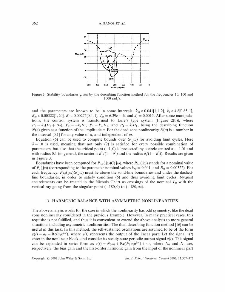
ExampleConsider again the electric motor example of Section 2, where the dead zone nonlinearity is nowconsidered asymmetric as in Figure 4, where b�40 and bþ50. The difference of having anasymmetric dead zone nonlinearity is that now we need a dual describing function, given byN0ða0; a1Þ and N1ða0; a1Þ. In this case, the describing function is independent of the frequency,since the nonlinearity is memoryless. In addition, the function N1ða0; a1Þ take values in theinterval [0,1] for any real value of a0 and a1, and independently of the parameters b� and bþ.The easiest way to use Equation (7) in avoiding the existence of multiple equilibrium points andlimit cycles is to derive conditions over Gð joÞ to satisfy the second inequality, which is asufficient condition.

Figure 4. Asymmetric dead zone nonlinearity.



This second condition can be embedded in the QFT framework using (6), where the functionNða;oÞ is substituted by N1ða0; a1Þ ¼ ½0; 1�, a similar condition to the obtained in Section 2. As aresult, boundaries given in Figure 3 are not only valid for a symmetric dead zone, but also forany asymmetric dead zone.

4. FREQUENCY LOCUS FOR THE NONLINEAR BLOCK

Although the main objective of this work is to obtain frequency locus for the controller Gð joÞ,in the form of boundaries, however, in order to analyse the degree of robustness/conservativeness achieved, it may be interesting to consider the ‘frequency locus’ filled by thenonlinear block N . As the nonlinear frequency response is not a so clearly defined object as thelinear one, it will be an approximate object, but useful for interpretations.

In the example of Section 1, the dead zone can be represented by an arbitrary number in ½0; 1�,so that we can identify it with N ¼ ½0; 1� � R, a bounded intervalar uncertainty. The closed loopLðH;NÞ will not have limit cycles when (2) holds, or equivalently when Hð joÞ=�N�1, or:

Hð joÞ \ �N�1 ¼ Hð joÞ \ ð�1;�1� ¼ | ð8Þ

Thus the linear part Hð joÞ must avoid the critical locus �N�1 ¼ ð�1;�1�. It should benoticed that this property, derived from the describing function, is shared by many otherdifferent nonlinear blocks, including the asymmetric dead zone, for which the first harmonic isreal between 0 and 1. For example, the unit saturation also has the ‘frequency locus’ N ¼ ½0; 1�and ‘critical locus’ �N�1 ¼ ð�1;�1�. The stability (lack of limit cycles) of the loop LðH;NÞ isbased on Hð joÞ avoiding the same locus, for N being the (symmetric or asymmetric) dead zoneas well as the saturation. So, there is some kind of approximation in this approach. Otherwise,the set of all stable linear HðsÞ will be unable to discriminate dead zone and saturation, in thesense that HðsÞ with a dead zone is stable if and only if HðsÞ with a saturation is stable, whichseems a rather unlikely property.

The validity of this ‘frequency locus’ analysis for such nonlinear blocks is strongly confirmedby the well-known validity of the harmonic balance principle for most of common practicalcases (in which Hð joÞ introduces a suitable low-pass effect). An additional way to increasesecurity in the guaranteed stability is to define a robustness gap as in (5). Putting L ¼ HN,omitting arguments for Hð joÞ and Nða;oÞ, and putting e ¼ 1=d, then (5) amounts to

j1þ ðHNÞ�1j > e

ðHNÞ�1 =2 � 1þ eU

H =2 N�1ð�1þ eUÞ�1 ¼ ð�N�1Þð�1þ eUÞ=ð1� e2Þ

ð9Þ

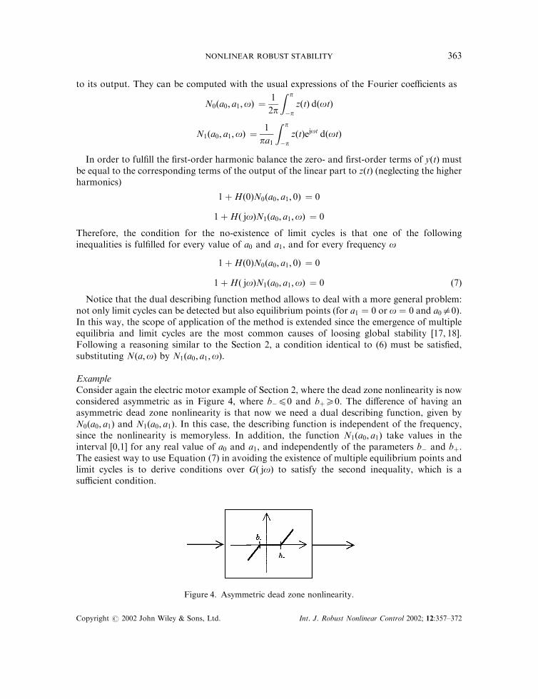
where U stands for the unit circle in the complex plane. Equation (9) shows the effect ofintroducing a robustness gap d ¼ 1=e in (5) on the forbidden critical locus: �N�1 is changed byð�N�1Þð�1þ eUÞ=ð1� e2Þ. Thus, each point z in the critical locus is changed by a forbiddencircle, centred at z=ð1� e2Þ, and with radius jzje=ð1� e2Þ. The union of all these circles forms the‘robust’ critical locus. Figure 5 shows this locus for the unit saturation and dead zone, fordifferent values of d ¼ 1=e.

It is worthwhile to analyse the relationship with other robust frequency bounds for L ¼ HNthat have been proposed in the literature. For example, in Reference [19] the closed-loop region

A. BANOS ET AL.364


for L=ð1þ LÞ is a rectangle, instead of a circle as in (5). In this case, it can be seen that thecorresponding open-loop condition is L ¼ HN =2 C where C is a clover, formed by the union offour circles centred at �1� r=2 and �1� jr=2 and with radius r=2, where d ¼ 1þ 1=r is therectangle half-width. Then, the locus for H takes the form H =2 ð�N�1ÞC, where C is the givenclover. In fact, this locus is introduced to simplify the performance monitoring, which is not ourapproach, so we will consider (5) as an adequate robustness bound and frequency loci as inFigure 5.

5. COMPARISON WITH ABSOLUTE STABILITY CRITERIA

An interesting question is about the comparison between the harmonic balance principle asdeveloped in Sections 2 and 3, and robust absolute stability criteria. The former givesapproximated solutions to the global stability problem, while the latter gives rigorous solutionsat the cost of being much more conservative. Robust absolute stability in the framework of QFThas been developed in References [1, 2]. In this section, we only consider memorylessnonlinearities like the dead zone example of Section 2 or Section 3, which have the propertyof lying incrementally in ½0; 1�. A memoryless nonlinear system N given by a relation y ¼ f ðxÞ issaid to lie incrementally inside the sector ½k1; k2� if k14½ f ðxÞ � f ðx0Þ�=ðx� xÞ04k2, for everyx; x0 2 R. Our sense of I/O stability is finite gain L2 stability. More formally, a system H :L2;e !L2;e is finite gain L2 stable if for every input x 2 L2, the output y ¼ Hx is in L2 and, in addition,jjyjj25kjjxjj2 for some constant k. Closed-loop stability is defined as I/O stability from any inputentering additively to the feedback system to the rest of signals. For this type of nonlinearities,the Circle and Popov Criteria used in Reference [1] are generalized using a minor modificationof multiplier stability conditions, as found in References [13] or [12]. The main result is:

Figure 5. Critical locus for the unit saturation and dead zone.



TheoremThe system LðH;NÞ, where H is given by (3), is stable if (i) HðsÞ is stable, (ii) N is static, odd,and lies incrementally in ½0; 1�, (iii) for some (possibly non-causal) WðsÞ, with impulse responsewðtÞ with L1 norm bounded by jjwðtÞjj151, condition (6) holds for any a; o 2 R, where

Nða;oÞ ¼ � �1þja

1�Wð joÞ

� ��1

ð10Þ

and (iv) if N is not odd then additionally wðtÞ > 0 for any t 2 R.

ProofThe proof is a minor modification of Theorem 11 in [13], where condition (iii) was based on theinequality

Reðð1�Wð joÞðHð joþ 1ÞÞ > e ð11Þ

The limit condition Reðð1�Wð joÞðHð joÞ þ 1ÞÞ ¼ 0 defines a boundary for Hð joÞ. Thisboundary can be obtained solving the equation 1�Wð joÞðHð joÞ þ 1Þ ¼ ja for any a 2 R. Aftersome simple manipulations the result is

1� �1þja

1�Wð joÞ

� ��1

Hð joÞ ¼ 0

or 1þNða;oÞHð joÞ ¼ 0, where Nða;oÞ is given by (10). Finally, from this last condition, it isstraightforward to prove that if (6) holds for this Nða;oÞ, then the original condition (11) issatisfied (note that there is an extra degree of robustness given by the parameter d in (6)). &

Following Section 4, this theorem can be interpreted in terms of a stabilizing nonlinearfrequency locus N given by (10), or a critical locus given by �N�1, that is

�N�1ða;oÞ ¼ �1þja

1�Wð joÞð12Þ

that, in general, are frequency-dependent. For each frequency o, the critical locus as given by(12) can be represented in the complex plane as straight lines passing through the �1 point,while the nonlinear frequency locus are circles.

Although the above theorem is a reformulation of a previous result, this new view isimportant, because it integrates under condition (6) multiplier results (that includes Circle andPopov Criteria) with the describing function method. Furthermore, that condition can betreated in the form of QFT boundaries. Thus, QFT gives a very natural framework for theanalysis and synthesis of stabilizing controllers using those methods.

5.1. Comparison of frequential and critical locus

Note that for WðsÞ ¼ 0 (no multiplier), we recover the classical (and very conservative) boundfrom the circle criterion, the complex half-space ReðzÞ5� 1. In general, the only influence ofWðsÞ in the complex plane over the nonlinear frequency locus is to rotate the bound ReðzÞ ¼ �1with an angle given by the phase of ð1�Wð joÞÞ. By finding appropriate multipliers Wð joÞ, theconservative bound given by the Circle Criterion can be remarkably relaxed. An interestingquestion is how much it can be relaxed, and how close to the describing function locus ð�1;�1�

A. BANOS ET AL.366


can be. Results in this line will clarify the limits of conservative for both the describing functionand the multiplier techniques.

The main difficulty is that the search space of possible multipliers WðsÞ is infinite-dimensional.This was arranged in Reference [14] in the context of antiwindup design, introducing aparticular, parameterized family of multipliers in the form

WðsÞ ¼a0

sþ 1þ

a1

ðsþ 1Þ2þ � � � þ

b0

s� 1þ

b1

ðs� 1Þ2þ � � � ð13Þ

For values of Wð joÞ close to zero, N as given in (10) approaches the complex circle around½0; 1� (Circle Criterion). However, when 1�Wð joÞ introduces a phase shift N becomes an off-axis circle, that will be referred to as CW ðoÞ. For stability based on multipliers, the graph of�H�1ð joÞ must avoid the circle CW ðoÞ, and for stability based on harmonic balance �H�1ð joÞmust avoid the real segment ½0; 1� � CW ðoÞ. But when �H�1ð joÞÞ lies on the lower (upper)half-plane, it is expected that the circle CW ðoÞ can be moved up (down) enough so thatthe forbidden region on the current half-plane is very close to ½0; 1�. In this case, the excessof conservatism given by the Circle Criterion can be minimized using appropriatemultipliers.

From (10), it is easy to obtain that the centre cðoÞ and the radius rðoÞ of CW ðoÞ are given by

cðoÞ ¼ 0:5ð1þ j tanðfðoÞÞÞ

rðoÞ ¼ jcðoÞj ð14Þ

where fðoÞ ¼ Angleð1�Wð joÞÞ. Note that at frequencies, where Wð joÞ is real, there is nophase shift, that is f ¼ 0, and we recover the circle of the Circle Criterion. Figure 6 shows thefrequency nonlinear locus for a nonlinearity satisfying the conditions of the above theorem, and

Figure 6. eft: Phase shift for the multiplier WðsÞ ¼ 0:3ð1=ðsþ 1Þ þ 1=ðs� 1ÞÞ, right: associated critical locus.



for

WðsÞ ¼ 0:31

sþ 1þ

1

s� 1

� �:

It is shown that the angle introduced by the multiplier as well as the boundaries for Hð joÞ in thecomplex plane. On the other hand, Figure 7 shows circles CW ðoÞ. Once the multiplier Wð joÞ isfixed and N is identified with the complex locus defined by the circles cðoÞ þ rðoÞU given by(14), it is straightforward to obtain boundaries for Gð joÞ. It suffices to apply the inequality (6)with N given by the family of circles.

5.2. Choice of positive multipliers

In this method, there is, in general, an infinite set of multipliers WðsÞ, which could be candidatesfor proving stability of a given system. The only condition required for WðsÞ in the theorem isthat jjwðtÞjj151. Considering the structured family given in (13) and assuming for simplicitywðtÞ50, the condition jjwðtÞjj151 is equivalent to [3]:

a0 � a1o2 þ a2o4 þ � � � þ ð�1Þmamo2m50 ð15Þ

b0 þ b1o2 þ b2o4 þ � � � þ bmo2m50 ð16Þ

ða0 þ b0Þ þ ða1 � b1Þ þ ða2 þ b2Þ2!þ � � � þ ðam þ ð�1ÞmbmÞm!51 ð17Þ

for all o. A first approach to the selection of WðsÞ could be based on linear matrix inequalities(LMI). If the controller Gð joÞ is given, then also Hð joÞ is given and the closed-loop stability bymultiplier techniques can be reduced to a set of LMIs, as in Reference [3].

However, it is not clear how the LMI method could be adapted in the case that the plantblocks PiðsÞ (i ¼ 1–4) contain arbitrarily shaped uncertainty, which is the approach in our work.

Figure 7. Frequency locus using the multiplier WðsÞ ¼ 0:3ð1=ðsþ 1Þ þ 1=ðs� 1ÞÞ.

A. BANOS ET AL.368


Furthermore, there is no need to postulate a possible controller Gð joÞ and then check by LMIsif it stabilizes the loop. We are more interested in leaving Gð joÞ unknown and obtainingboundaries for it, within the QFT framework. Let us see some ideas in this line. The vector ofmultiplier parameters is

p ¼ ðp1; p2; . . . ; p2mþ2Þ> :¼ ða0; a1; . . . ; am; b0; b1; . . . ; bmÞ

>

Let 1�WpðsÞ be the multiplier for the parameter choice p 2 R2mþ2. Then, the phase shiftintroduced by the multiplier is

fðo; pÞ ¼ Angleð1�Wpð joÞÞ

Note that as discussed above, applying the multiplier theorem is equivalent to modelling thenonlinearity N by a frequency-dependent complex locus. A first question in multiplier search isif some multipliers are, in general, ‘better’ or ‘worse’ than others, in the sense that for twochoices p= *pp, the complex circles are such that Cðo; pÞ � Cðo; *ppÞ for all o. It can be seen thatthis never happens and that there are no maximal or privileged multipliers, in general. To prove it,recall that the circles are actually dependent on the phase Cðo; pÞ :¼ Cðfðo; pÞÞ and, by the formof WpðsÞ, different parameters produce different phase curves: p= *pp ) fð�; pÞ=fð�; *ppÞ. Thus,different parameters produce different circle families.

A second interesting aspect is to consider a perturbation analysis: If a multiplier withparameters p 2 R2mþ2 is fixed as a basic or central solution, which is the effect of a smallperturbation dp 2 R2mþ2 on the circles Cðo; pþ dpÞ?.

Some possible ways to deal with this question will be outlined now. In the field of QFT, it iscustomary to work with a finite set of frequencies fo1;o2; . . . ;ong (e.g. f1; 10; 100g rad=s). Thissimplifies drastically the problem. Put, for 14k4n:

fkðpÞ ¼ Angleð1�Wpð jokÞÞ; fðpÞ ¼ ðf1ðpÞ; . . . ;fnðpÞÞ>

Then, by smoothness of the function fðpÞ, it can be assured that there exists an n� ð2mþ 2Þmatrix F such that:

dfðpÞ :¼ fðpþ dpÞ � fðpÞ � F dp

for small perturbations. After some lengthy but straightforward manipulation, putting:

WðsÞ ¼a0

ðsþ 1Þþ � � � þ

bm

ðs� 1Þmþ1:¼ p1g1ðsÞ þ � � � þ p2mþ2g2mþ2ðsÞ

which defines implicitly the systems glðsÞ, it can be proved that the ðk; lÞ entry of F is:

ðFÞkl ¼ �Realfglð jok=ð1�Wpð jokÞÞg

Notice that, at a given frequency ok, there is a single degree of freedom available concerningthe circle for ok. This degree of freedom is manipulated by changing the phase shift fkðpÞ. Then,in order to be able to simultaneously exploit all the n degrees of freedoms at all the QFTfrequencies ok, it suffices (i) that the matrix F has full column rank n and (ii) that all theperturbations dp around the current multiplier parameters p are feasible (i.e. satisfy conditions(15)–(17)).

The first property is expected to be satisfied generically (i.e. except around special or singularvalues of p) provided that 2mþ 2 n. In other words, including a large enough number 2mþ 2of multiplier coefficients, the full column rank n 2mþ 2 for F will be finally reached.



The second property is satisfied whenever (M1) and (M2) are satisfied by p in a non-marginalway (i.e. the ‘50’ symbols are in fact ‘> 0’). In this case, there is an open set such that pþ dp isalso feasible for all directions dp of a small enough perturbation jjdpjj ! 0.

This can be summarized in the following property: If a vector of 2mþ 2 multiplier coefficientsp is given, and it is feasible in a non-marginal way, then for large enough m, every n-vector dfðpÞof phase perturbations (influencing the QFT boundaries) can be obtained by an adequateperturbation dp of the multiplier coefficients. In a few words, for every small df, there existssome dp such that df ¼ F dp.

The previous ideas give the sketch of a technique for finding multipliers to prove stability ofthe feedback loop. The implicit scope question is: If a controller GðsÞ is such that it makes theclosed loop stable (and this is checked by describing function or any other method), will it bepossible to prove stability also by multiplier techniques? In other words, can we find a multiplierfor proving stability of every stable system?

It is not clear how to give an affirmative answer in general. However, experiences with manyexamples of common control systems suggest that the answer could be yes in many practicalcases. The discussion above also outlines an approach for finding the multiplier. Furthermore, itshould be said that the QFT framework facilitates drastically the problem, due to the inherentdiscretization fokgk of the frequency axis. In addition, QFT gives a very natural framework forthe design of appropriate multipliers, using the preceding interpretation of 1�Wð joÞ as aphase shifter for every frequency o. In a particular case, the designer can easily detect thefrequency range in which the multiplier has to maximize the phase shift, using as starting pointthe case of no multiplier ðWð joÞ ¼ 0Þ and concentrating in the frequencies corresponding to themost demanding boundaries, trying to minimize the compensator bandwidth, and using theboundaries given by the describing function method as a guide. This has been the approachfollowed in the following example.

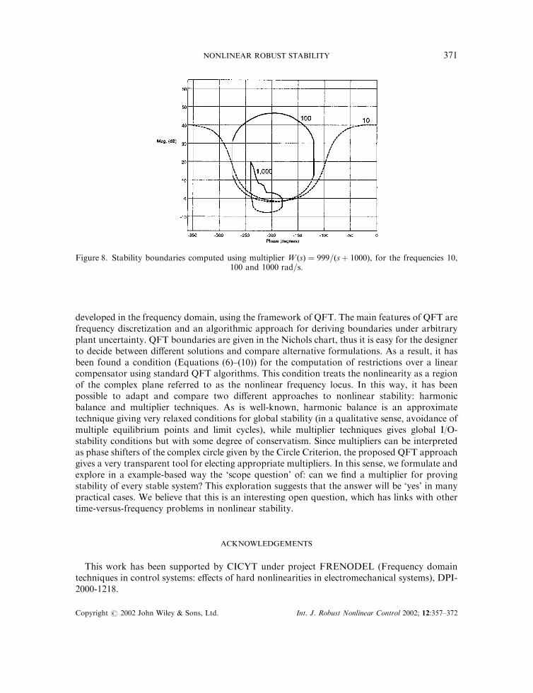
ExampleFor the electric motor example of Section 2, application of the stability theorem based onmultipliers is valid for both the symmetric and asymmetric dead zone nonlinearity, since theyare static, and lies incrementally in ½0; 1�. The multiplierWðsÞ ¼ 999=ðsþ 1000Þ has been chosen,because it provides a phase shift of almost 90 between 10 and 100 rad=s. In fact,1�WðsÞ ¼ ðsþ 1Þ=ðsþ 1000Þ is a lead network. Results are given in Figure 8. Boundarieshave been computed for P3;0ð joÞGð joÞ, where P3;0ð joÞ stands for a nominal value of P3ð joÞ.Note that for every frequency, P3;0ð joÞGð joÞ must lie above the solid-line boundaries and underthe dashed-line boundaries.

Boundaries of Figure 3, given by the describing function method, can be used as a guide tomeasure how good is a multiplier, if the resulting boundaries are close to them. In this sense, onemay conclude that the chosen multiplier give reasonable results, in the sense the correspondingboundaries, shown in Figure 8, are no overly conservative. Of course, a more rigorous study isneeded in order to formalize and systematize this procedure.

6. CONCLUSIONS

The problem of designing stabilizing linear compensators for uncertain nonlinear feedbacksystems has been addressed. A solution for a special type of nonlinear systems has been

A. BANOS ET AL.370


developed in the frequency domain, using the framework of QFT. The main features of QFT arefrequency discretization and an algorithmic approach for deriving boundaries under arbitraryplant uncertainty. QFT boundaries are given in the Nichols chart, thus it is easy for the designerto decide between different solutions and compare alternative formulations. As a result, it hasbeen found a condition (Equations (6)–(10)) for the computation of restrictions over a linearcompensator using standard QFT algorithms. This condition treats the nonlinearity as a regionof the complex plane referred to as the nonlinear frequency locus. In this way, it has beenpossible to adapt and compare two different approaches to nonlinear stability: harmonicbalance and multiplier techniques. As is well-known, harmonic balance is an approximatetechnique giving very relaxed conditions for global stability (in a qualitative sense, avoidance ofmultiple equilibrium points and limit cycles), while multiplier techniques gives global I/O-stability conditions but with some degree of conservatism. Since multipliers can be interpretedas phase shifters of the complex circle given by the Circle Criterion, the proposed QFT approachgives a very transparent tool for electing appropriate multipliers. In this sense, we formulate andexplore in a example-based way the ‘scope question’ of: can we find a multiplier for provingstability of every stable system? This exploration suggests that the answer will be ‘yes’ in manypractical cases. We believe that this is an interesting open question, which has links with othertime-versus-frequency problems in nonlinear stability.

ACKNOWLEDGEMENTS

This work has been supported by CICYT under project FRENODEL (Frequency domaintechniques in control systems: effects of hard nonlinearities in electromechanical systems), DPI-2000-1218.

Figure 8. Stability boundaries computed using multiplier WðsÞ ¼ 999=ðsþ 1000Þ, for the frequencies 10,100 and 1000 rad=s.



REFERENCES

1. Ba *nnos A, Barreiro A. Stability of nonlinear QFT designs based on robust absolute stability criteria. InternationalJournal of Control 2000; 73(1):74–88.

2. Barreiro A, Ba *nnos A. Nonlinear robust stabilization by conicity and QFT techniques. Automatica 2000; 36(9):3. Horowitz I. Survey of quantitative feedback theory (QFT). International Journal of Control 1991; 53(2):255–291.4. Horowitz I. Synthesis of feedback systems with nonlinear time-varying uncertain plants to satisfy quantitative

performance specifications. IEEE Transactions on Automatic Control 1976; 20(4):454–464.5. Horowitz I, Ba *nnos A. Fundamentals of Nonlinear QFT. In Advances in Nonlinear Control System, Ba *nnos A,

Lamnabhi-Lagarrigue F, Montoya FJ (eds). Springer: London, 2001.6. Oldak S, Baril C, Gutman PO. Quantitative design of a class of nonlinear systems with parameter uncertainty.

International Journal of Robust and Nonlinear Control 1994; 4:101–117.7. Wang TS, Hwang YC, Tsai TP. Synthesis of feedback control systems with large plant uncertainty and time-varying

gain. International Journal of Control 1990; 51(3):687–704.8. Mees AI. Dynamics of Feedback Systems. Wiley: New York, 1981.9. Khalil HK. Nonlinear Systems. Prentice-Hall: Upper Saddle River, NJ, 1996.10. Vidyasagar M. Nonlinear Systems Analysis. Prentice-Hall: Englewoods Cliffs, NJ, 1978.11. Eitelberg E, Boje E. Some practical low frequency bounds in quantitative feedback theory. Proceedings of the

ICCON’89 WP-2-1 1989; 1–5.12. Megretski A, Rantzer A. System analysis via integral quadratic constraints. Automatica 1997; 42:819–830.13. Kothare MV, Morari M. Multiplier theory for stability analysis of anti-windup control systems. Automatica 1999;

35:917–928.14. Horowitz I. Quantitative Feedback Design Theory (QFT). QFT Publications: Boulder, CO, 1993. This is available (in

America) from I. Horowitz: [email protected], and elsewhere from A. Ba *nnos: [email protected]. Chait Y, Yaniv O. MISO computer-aided control design using the Quantitative Feedback Theory. International

Journal of Robust and Nonlinear Control 1993; 3:47–54.16. Cook PA. Nonlinear Dynamical Systems. Prentice-Hall: Englewood Cliffs, 1986.17. Cuesta F, Gordillo, F, Aracil J, Ollero A. Global stability analysis of a class of multivariable Takagi–Sugeno fuzzy

control systems. IEEE Transactions on Fuzzy Systems 1999; 7(5):508–520.18. Gordillo F, Aracil J, Ollero A. Robust stability analysis of MIMO systems with asymmetric nonlinearities.

Proceedings of the 14th World Congress of IFAC, Vol. E, 1999; 123–127.19. Gustafsson F, Graebe SF. Closed loop performance monitoring in the presence of system changes and disturbances.

Automatica 1998; 34:1311–1326.

A. BANOS ET AL.372


A QFT framework for nonlinear robust stability

Documents