A probability-weighted moment test to assess simple scaling

Stochastic Hydrology and Hydraulics 8, 173-183 © Springer-Verlag 1994

A probability-weighted moment test to assess simple scaling

Praveen Kumar Universit ies Space Research, Association/Hydrological Sciences Branch, NASA-Goddard Space

Flight Center, Greenbelt, MD 20771, USA

Peter Guttarp Depar tment o f Statistics, University o f Washington, Seattle, WA 98105, U S A

Eft Foufoula-Georgiou St. Anthony Falls Hydraulic Lab, Department o f Civil Engineering, University o f Minnesota, Minneapolis , M N 55414, U S A

Abstract: We present a statistically robust approach based on probability weighted moments to assess the presence of simple scaling in geophysical processes. The proposed approach is different from current approaches which rely on estimation of high order moments. High order moments of simple scaling processes (distributions) may not have theoretically defined values and consequently, their empirical estimates are highly variable and do not converge with increasing sample size. They are, therefore, not an appropriate tool for inference. On the ether hand we show that the probability weighted moments of such processes (distributions) do exist and, hence, their empirical estimates are more robust. These moments, therefore, provide an appropriate tool for inferring the presence of scaling. We illustrate this using simulated Levy- stable processes and then draw inference on the nature of scaling in fluctuations of a spatial rainfall process.

Key words: Probability weighted moment, scaling in rainfall, stable distribution,

1 I n t r o d u c t i o n

The range of spatial and temporal scales for which geophysical models are developed and used is quite broad. Lately" much interest has focused on questions of sealing properties of geophysicM processes (see for example, Meakin, 1991). From a statistical and physical staaadpoint, the most important aspect of the notion of scaling is that the probability distribution of the phenomenon is invariant with respect to a function cA, where A is a scale parameter. If X(s) denotes a simple scaling process, where s is a temporal or spatial index, then [Lamperti, 1962] for any A > 0 there is a constant cA such that

caX(~s) d= X(s) (1)

where d stands for equality in distribution. By repeated application of equation (1) we see that c~A~ = c ~ c ~ , hence c~ = A -H. Tile quantity H is called the scaling exponent or characteristic exponent, which can be positive or negative. Since (t) is valid both for magnification (A <: 1) and contraction (A > 1), inference about a simple scaling process can be made from a large scale, where it may be easily observable, to very small scales, for which observations may be difficult or impossible to 0btain~ or vice versa.

Often, the analysis of scaling hydrological processes towards assessing their scaling properties has been done using empirical moments (see for example Gupta and Waymire, 1990). Define the rescaled process X~ by

X~(s) = X(~s) . (2)

174

If a scaling process has moments of order k, then for any s

E[X~(s)] = ~ [ X ~ ( s ) ] . (3)

tlence, a log-tog plot of empirical moments against scale should show a straight line (if the moments are negative, one can use the real part of the logarithm). However, a large class of processes that are simple scaling have a marginal distribution of the stable type (Zolotarev [1986] has an exhaustive treatment of these distributions). The stable distributions, with the exception of the normal, do not possess moments of order above 2 (in fact, they possess only moments of order less than c~, where c~ is the order of the stable distribution). The stable processes (with fractional Brownian motion as a special case) are the most commonly encountered simple scaling processes.

Studies such as those in Gupta and Waymire [1990] use estimation of high order moments from the data to look for scaling. From a statistical point of view, there are two problems with this. First, high order empirical moments are dominated by large observations, and are therefore highly variable. In fact, it is possible that their results on the scaling properties of rainfall may be driven entirely by a few large observations. In statistical terms, the empirical moments about zero are highly non-robust against outliers. Second, high order sample moments from a non-normal stable distribution, which, in essence, a t tempt to estimate infinite parameters, have infinite mean and variance. Thus, they are inherently very unreliable and do not converge with increasing sample size (see Mandelbrot, 1963).

In order to obtain a statistically more satisfying test for assessing the presence of scaling in geophysical process, we employ the probability weighted moments (PWMs) of Greenwood et al. [1979] and tIosking [1986]. We show that these moments are welt defined for most of the stable distributions, and their estimators are more robust against outliers than are standard empirical moments. Moreover, probability weighted moments are more amenable to estimation of standard errors and, therefore, provide an objective method of judging the performance of the estimates and inferences about scaling. Taking into account the uncertainties in estimated quantities (e.g., fractal dimension or scaling exponent) and translating that into a standard error is a very important aspect of the assessment of scaling properties of a physical process. Unfortunately, most of the literature ignores the consequences of inexact measurements and assumes that the properties of the studied field can be measured exactly. Only recently there is some work in the statistical literature where box counting estimates of fractal dimension are assessed assuming a stochastic underlying random field [Hall and Wood, 1993; Ogata and Katsura, 1991].

The objective of this paper is to develop a technique using probability weighted moments for the identification of simple scaling. In section 2 of the paper we derive the behavior of PWMs under simple scaling, and discuss the estimation of PWMs and their standard errors of estimates. Section 3 contains results from applying these methods to simulated scaling Levy-stable processes, and to rainfall intensities and their fluctuations as derived in Kumar and Foufoula-Georgiou [1993a,b]. The rainfall field is used only to illustrate the applicability of PWMs to assess scaling in geophysical fields. The complete characterization of the scaling behavior in rainfall can be found in Kumar and Foufoula-Georgiou [1993a,b]. Finally in section 4 we discuss possible extensions of the methodology.

2 Sca l ing a n d p r o b a b i l i t y w e i g h t e d m o m e n t s

For a random variable X with cumulative distribution function Fx having E[tXI] < oo, Greenwood et al. [1979] defined probability weighted moment of X as

PWM(i, j , k) = E[Xi{Fx(z)} j {1 - Fx(z')} k]

= J z i { F x ( z ) } J { 1 - Fx(x)} k dFx(z) . (4)

This can alternatively be written as

1

PWM(i , j ,k ) = /{z(Fx)} iFJx(1 - Fx)kdFx (5)

0

where x(Fx) is the quantile thnetion. PWM(i,0,O) are the conventional non-central moments. We will work with PWM(1j ,k) into which X enters linearly, and in particular with quantities ak and flk as defined below:

175

oo

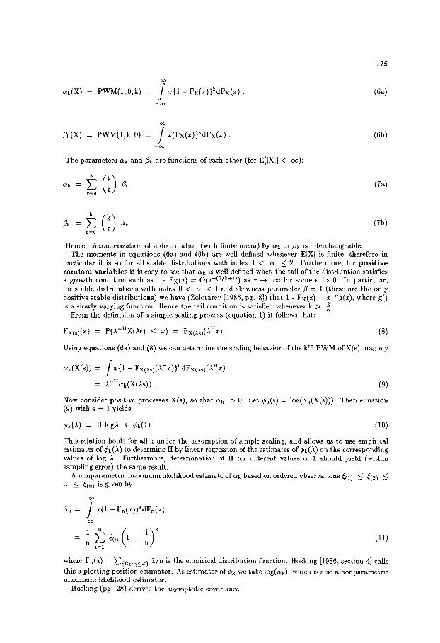
ak(X) ---- PWM(1,0 , k) = / x { 1 - F x ( x ) } k d F x ( x ) .

- o o

(6a)

7 ~k(X) ~-- PWM(1,k,O) = / x ( F x ( x ) } k d F x ( x ) .

- c o

The parameters ~k and ~k are functions of each other (for E[IXI] < oc):

r=0 \ r /

(6b)

(7a)

( )Or /Tb/ r = 0

Hence, characterization of a distribution (with finite mean) by ak or fik is interchangeable. The moments in equations (6a) and (6b) are well defined whenever EIX I is finite, therefore in

particular it is so for all stable distributions with index 1 < a < 2. Furthermore, for p o s i t i v e r a n d o m v a r i a b l e s it is easy to see tha t ak is well defined when the tail of the distr ibution satisfies a growth condition such as 1 - Fx(x) = O(z -(2/k+C)) as x --~ oo for some e "> 0. In particular, for stable distributions with index 0 < a < 1 and skewness parameter fl = 1 (these are the only positive stable distributions) we have (Zolotarev [1986, pg. 8]) tha t 1 - Fx(z) = z-~g(x), where g0 is a slowly varying function. Hence the tail condition is satisfied whenever k > ~.

From the definition of a simple scaling process (equation 1) it follows that :

Fx(s)(z) = P(A-HX(,~s) < x) = rx(~s)(~Hx) (8)

Using equations (6a) and (8) we can determine the scaling behavior of the k th PWM of X(s), namely

O / k ( X ( s ) ) = . /X{1 - Fx(~s) ()~Hx)}k dFx(~s)(),H x)

= A-H~k(X(As)) . (9)

Now consider positive processes X(s), so tha t ~k > O. Let ek(s) ---- log(~k(X(s))). Then equation (9) with s = 1 yields

e k ( ~ ) = H | O g ~ -~- Ok(l) (10)

This relation holds for all k under the assumption of simple scaling, and allows us to use empirical estimates of ek(~) to determine H by linear regression of the estimates of ek(A) on the corresponding values of log ,~. Furthermore, determination of H for different values of k should yield (within sampling error) the same result.

A nonparametr ic maximum likelihood estimate of ak based on ordered observations ~0) -< ~(~) .-- <_ ~(n) is given by

&k = 7 x(1 -- Fn(x) )kdF, (x)

i)k = - ~0) 1 - (11)

n i=l

where F~(x) -- ~{i:~(,)_<~} 1/n is the empirical distribution function. Hosking [1986, section 4] calls this a plot t ing position estimator. As est imator of ek we take log(&k), which is also a nonparametr ie maximum likelihood estimator.

Hosking (pg. 28) derives the asymptotic eovariance

176

ajk = AsCov(&k,&j)

_- _In i J(I-F(x))k(I-F(Y))JF(x)(I-F(y))dx dy x<y

Ijk/n (12)

We estimate ajk by replacing the cdf F(z) by the empirical distribution function Fn(r). Using standard Taylor series arguments the asymptotic variance for Ck is given by Ikk/(na~).

In order to estimate H from Ck(),), we need to take into account the fact that the estimates Ck have different variance for different values of ,1. Using (8) and (12) we can derive the formula

Ijk(~ ) = tjk(1)/.~ -2H , (13)

so the asymptotic variance of tk (A) is Ikk (1)/(nacre(I)) where n~ is the sample size at scale A. Hence, we estimate tI (for a given value of k) by a weighted regression, using weights inversely proportional to the asymptotic variance, or, equivalently , proportional to the sample size. We estimate the standard error of H from the regression in the usual fashion. This estimate is likely to be too small, since there is positive dependence between the tk(A) for different values of A. An improved regression would take these.covarianees into account, but it is difficult to derive expressions for them.

For symmetric distributions ~k tends to be negative and /3 k positive, and it is there[ore more convenient to use /3k for analysis. It is noted that for positive stable random variables, only C~k exists provided k is large enough, but not ilk, and vice-versa. Estimates of flk and their asymptotic properties are derived in the same fashion as those for C~k above. For example, a nonparametric maximum likelihood estimate of ilk based on ordered observations ~(1) _< ~(~) _< ... _< ~(n) is given by

flk = f x (F , (x ) )kdF, (x)

(g = - ~(i) (14) n i : l

The asymptotic covarianee is

1 AsCov(~k, ]~ j )=

x<y

A scaling relationship analogous to equation (9) also holds, viz,

/3k(X(s)) = ~ -nZk(X(~s) ) . (16)

3 A p p l i c a t i o n s

In this section we apply the developed methodology to two different cases: fluctuations of a simulated Levy stable process (including Brownian motion obtained as a special case for a = 2), and rain rates and their fluctuations for a severe squall line storm in Oklahoma.

3.1 Levy stable process

A Levy stable process is defined as a process that has self-similar, stationary, independent increments having a stable distribution. For such processes the scaling exponent is given as H = 1/a . The ease of a- = 2 gives the usual Brownian motion process.

Let s be a time parameter, and X(s) fluctuations of a Levy stable process. Levy stable process was simulated over 2048 points. Averages of two adjacent non-overlapping values provided the Levy sta- ble process at the next coarser scale (1024 points) and differences of adjacent non-overlapping values provided the fluctuation process at that same scale. This procedure of averaging and differencing was repeated at coarser and coarser scales resulting in the Levy stable process and its fluctuation process at several scales.

177

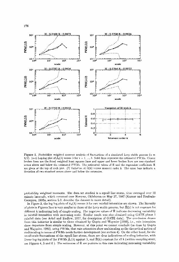
Figures la-e and 2a-e show the log-log plots of ~k(,~) versus ,~ for k = 1, ..., 5 for fluctuations of Levy stable process for a = 3/2 and a = 2 (Brownian motion), respectively. The plots are, as expected, close to linear. The confidence lines in Figures la-e and 2a-e are two individual standard errors above and below the estimate. For each value of k we estimated H(k) by weighted linear regression, as outlined in the previous section. Figures If and 2f show I:I(k) plotted against moment order k, together with bars that reach two estimated standard errors above and below I:I(k). The scaling behavior of the Levy stable process is clearly captured. The estimated value of H (approximately 0.57) for c~ = 3/2 is slightly( different from the theoretical value of 0.67. For the Brownian motion case the estimated value is very close to the true value (0.48 versus 0.5). It should be noted that the estimates of H for c~ = 3/2 appear statistically different from their true values. This is due to the conservative estimates of their standard error which ignores cross correlation of PW, Ms of different orders. If cross correlation was accounted for in the estimation of standard errors (something that seems difficult to accomplish analytically), it is conjectured that the estimates of H would not be statistically different from their true values, i.e., would be within 2 standard errors of estimate. Until this is shown however, we offer the PWM method not as a robust method for estimation of H but rather as a robust, method of inferring simple scaling. Several simulations for different values of c~ showed slight errors in estimates of H but never failed to capture the scMing behavior. That is, log-log linearity of PWMs with respect to scale and invariance of slope of these plots with respect to order of moments was always observed. The usual moment analysis failed to even show log-log linearity of moment with respect to scale establishing clearly that the PWM method is more robust for the identification of simple scaling behavior.

It is interesting to note that if the variability of PWM estimates at different scales had been ignored, and simple, instead of weighted, least squares had been used, the estimates of H would have been much more variable with respect to moment order k (although still with high correlation coefficients in the log-log regression of PWM versus scale).

3.2 Rainfall fluctuations in a squall line storm

Rainfall fields are always positive with an atom at zero, i.e., they have a non-zero probability of being zero. Kedem and Chin [1987] argued that the positivity of rain intensities and atom at zero, together, preclude the possibility of simple scaling on theoretical grounds. This, however, is not the case for rainfall fluctuations where the condition of positivity does not hold. The initial argument for this was provided by Lovejoy and Sehertzer [1989]. Later, Kumar and Foufoula~Georgiou [1993a,b] discussed why rainfall fluctuations are natural components to be tested for scaling. They used wavelet transforms to decompose rainfall intensities into large and small scale components representing the mean behavior of the process and fluctuations, respectively. This decomposition can be represented a s

X(s) = ~ ( s ) + X'(s) s = ( s l , s~ ) c a ~ (17)

where the mean process X(s) and fluctuation process X'(s) were approximated using scale functions and wavelets, respectively. The two components, i.e., mean and fluctuations, are uncorrelated as the decomposition is obtained using filters having non-overlapping frequency bands. This has also been verified through cross-correlation between X(s) and X'(s). Using separable orthogonat wavelets, the fluctuation process X'(s) was further decomposed into three components as X'(s) -- X~(S) + X~(s) + X~(s) which themselves are uncorrelated. X(s) represents the large scale behavior governing the morphological organization of the storm, and X~ (s)," X~(s) and X~(s) capture the horizontal, vertical and diagonal high correlations of the fluctuation process (these three components are henceforth referred to as D1, D2 and D3 components, respectively). The framework within which scaling was studied was in the sense of the followixlg equation:

(X~(As)} d (AHIX~(s)} i e [1,3] (18)

where the equality is in distribution. It was found that each component Xi showed scaling behavior up to a certain scale £max-

Using the above decomposition (with Haar wavelets), here we investigate the scaling properties of the raw intensities and small-scale fluctuation components {Xi}i=l ,2, 3 using the technique of

178

lO t -I 10 o

10-1 10 °

10~

10o

10-t 10o

H : 0.5468 R : 0,9873 /

, /

seal.=

H : 0.5757 R : 0.993.4

10t 102 10~ sca le

IO l

10 o

m i ~ o

101

- 100

10.1 100

H : 0.5708 R : 0.9926

101 102 103 .scale

H : 0.5764 R : 0,9935

101 102 103 scale

l 0 t

~ lO o

10-t 10 o

H : 0.5752 R : 0 . 9 9 3 2 /

/"

/

101 102 10 ~ scale:

E L~

Variation of H with k

0.8 ..................... i .................. ~ ..................

o . ~ ......... ~ . ~ . . . . . . ~ ........... i ........... t . . . . . . . . . .

o . 4 t- . . . . . . . . . . . . . . . . . . . . . . ~ . . . . . . . . . . . . . . . . . . . . . ; . . . . . . . . . . . . . . . . . . . . .

0.2 [ ~ . . . . . . . . . :: . . . .

0 . . . . i,,, 0 2 6

Moment order k

F i g u r e 1. Probability weighted moment analysis of fluctuations of a simulated Levy stable process (a = 3/2). (a-e) Log-log plot of ilk()0 versus ), for k = 1 ..... 5. Solid lines represent the estimated PWMs. Center broken lines are the fitted weighted least squares lines and upper and lower brokdn lines are two standard errors above and below the estimated PWMs. The estimated values of H and the regression coefficients R are given at the top of each plot. (f) Variation of ~](k) versus moment order k. The error bars indicate a deviation of two standard errors above and below the estimates.

p robab i l i t y weighted moments . The d a t a set s tud ied is a squa l l l ine s torm, t i m e averaged over 10 m i n u t e in tervals , which occurred over Norman , O k l a h o m a on May 27, 1987 ( K u m a r and Foufoula- Georgiou, 1993a, sect ion 5.2, describe the da t a se t in more detai l ) .

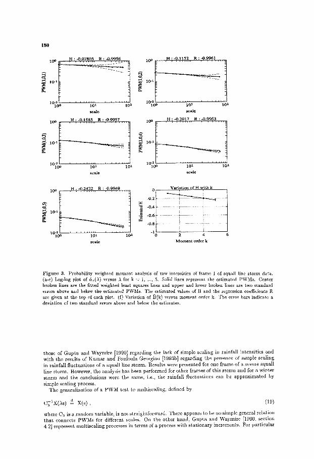
In F igure 3, the log-log plots of &k(A) versus A for raw rainfal l in tens i t ies are shown. The l inear i ty

of p lo ts fix F igures 3a-e is very s imi la r to those of the Levy s tab le process, bu t I:i(k) is not cons tan t for

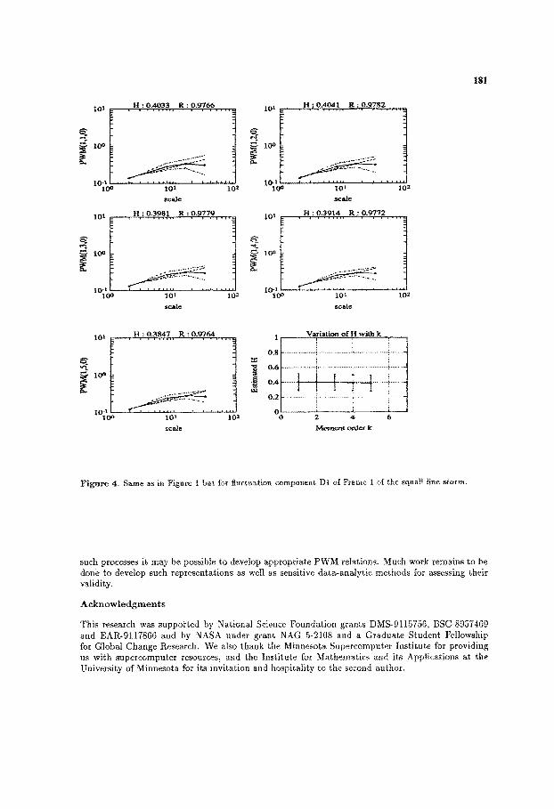
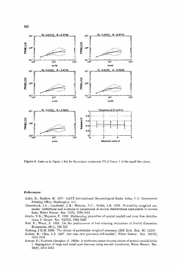
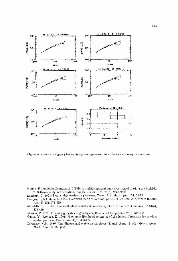
different k i nd ica t ing lack of s imple scal ing. The nega t ive values of I:t ind ica te decreasing var iab i l i ty in ra infa l l in tens i t ies wi th increasing scale. Similar resul t was also ob t a ined us ing G A T E phase 1 rainfal l d a t a (see Arkel and Hudlow, 1977, tbr descr ip t ion of G A T E data) . The conclusion drawn from th i s behav io r is s imi la r to those ob ta ined by G u p t a and Waymi re [1990], i.e., ra in in tens i t i es show depa r tu re f rom s imple scal ing. However, a t th is po in t we cannot conclude (as done by G u p t a and Waymire , 1990), us ing P W M s , t h a t ra in in tens i t ies show mul t i sca l ing as the theore t ica l no t ion of mu l t i s ea l ing in t e r m s of P W M s needs fur ther deve lopment (see sect ion 4). On the o ther hand , for the smal l -sca le f luc tua t ions of the squal l l ine s torm, there are clear ind ica t ions of scal ing behavior , w i th l inear log-log plots of the PWMs/~k (A) aga ins t ),, and t l (k) cons tan t for al l k (wi th in s a m p l i n g error;

see Figures 4, 5 and 6 ). The e s t ima tes of I~t are pos i t ive in this case ind ica t ing increas ing var iab i l i ty

101

10 o

mi~oo

I0~ I

lOl

"~'~" 10° I

mi'oo

H : 0.5253 R : 0.9965

101 10 2 10 3 scale

H : 0.4748 R : 0.9956

I0 ~, I0 2 I0 3 scale

H : 0.45 R : 0~994

101 102 I0 ~ scale

10 ~

I lO-i t 10 o

lot I

H : 0.493 R : 0.9963

10 ~ 102 10 a scale

H : 0.,,613 R : 0.9948

101 102 10 3 scale

Variation of H with k 1

0 ~ 0 2 4 6

Moment order k

179

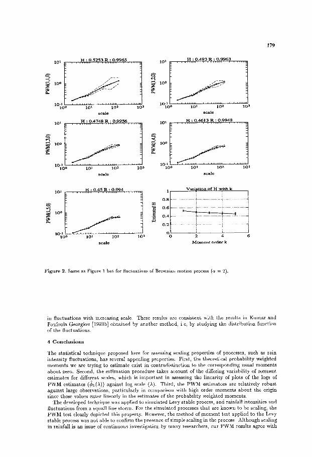
Figure 2. Same as Figure 1 but for fluctuations of Brownian motion process (a = 2).

in fluctuations with increasing scale. These results are consistent with the results in Kumar and Foufoula-Georgiou [1993b] obtained by another method, i.e, by studying the distribution function of the fluctuations.

4 Conc lus ions

The statistical technique proposed here for assessing scaling properties of processes, such as rain intensity fluctuations, has several appealing properties. First, the theoretical probability weighted moments we are trying to estimate exist in contradistinction to the corresponding usual moments about zero. Second, the estimation procedure takes account of the differing variability of moment estimates for different scales, which is important in assessing the linearity of plots of the logs of PWM estimates (¢k(A)) against log scale (A). Third, the PWM estimators are relatively robust against large observations, particularly in comparison with high order moments about the origin since these values enter linearly in the estimates of the probability weighted moments.

The developed technique was applied to simulated Levy stable process, and rainfall intensities and fluctuations from a squall line storm. For the simulated processes that are known to be scaling, the PWM test clearly depicted this property. However, the method of moment test applied to the Levy stable process was not able to confirm the presence of simple scaling in the process. Although scaling in rainfall is an issue of continuous investigation by many researchers, our PWM results agree with

180

H : -0 .0" /805 R : - 0 . 9 9 5 6 I 0 o j ~ . . . . . . . . . , . . . . . . . . . . . . . . . . w ~

~ ":~.~ _ -.- -..- .........

1 0 4

10i~0o 101 l 0 a

s ca l e

H : - 0 . 1 5 8 5 R : - 0 . 9 9 5 7

10 o 101 10 2

s c a l e

H : - 0 , 2 4 2 2 R : - 0 . 9 9 4 9 10 ° , • , , . . . . . . . . . . . . .

1 0 ~ , ~

lO . l

l 0 t 102

s c a l e

H : - 0 . 1 1 5 2 R : - 0 . 9 9 6 1 10 o , , . . . . . . . . . . . . . . .

lO_t . . . . . . . .

I 0 I0~ 'I0 :t s c a l e

H : - 0 . 2 0 1 7 R : - 0 . 9 9 5 3 10 o , . . . . . . . . . . . . . . .

i i0.i

10.2 z . . . . . I 0 o lO t l 0 2

s c a l e

V a r i a t i o n o f H w i t h k

--13.2. ......... _ _ .........

- 0 . 6 . . . . . . . . . . . . . . . . . . . . i ........................ i . . . . . . . . . . . . . . . . . . . .

-0.8 . . . . . . . . . . . . . ~ .. . . . . . . . . . . . . . . . . i . . . . . . . . . .

.1 i i 0 2 4 6

M o m e n t o r d e r k

Figure 3. Probability weighted moment anMysis of raw intensities of frame 1 of squall line storm data. (a-e) Log-log plot of G~(A) versus A for k = 1, ..., 5, Solid lines represent the estimated PWMs. Center broken lines are the fitted weighted least squares lines and upper and lower broken lines axe two standard errors above and below the estimated PWMs. The estimated values of H and the regression coefficients R are given at the top of each plot. (f) Variation of ~t(k) versus moment order k. The error bars indicate a deviation of two standard errors above and below the estirnates.

those of Gupta and Waymire [1990] regarding the lack of simple scaling in rainfall intensities and with the results of Kmnar and Foufoula-Georgiou [1993b] regarding the presence of simple scaling in rainfall fluctuations of a squall line storm. Results were presented for one frame of a severe squall line storm. However, the analysis has been performed for other frames of this storm and for a winter storm and the conclusions were the same, i.e., the rainfall fluctuations can be approximated by simple scaling process.

The generalization of a PWM test to multiscaling, defined by

C ; l X ( A s ) ~ - X ( s ) , ( 1 9 )

where C~, is a random variable, is not straightforward. There appears to be no simple general relation that connects PWMs for different scales. On the other hand, Gupta and ~¥aymire [1990, section 4.2] represent multiscaling processes in terms of a process with stationary increments. For particular

I 0 t

1 0 4 10 o

l O t

lO-X I 0 o

H : 0 . 4 0 3 3 R : 0 . 9 7 6 6

101 10 a

s c a l e

H : 0 . 3 9 8 1 R : 0 . 9 7 7 9

l O l 102

scale

10 t . H . : 0 . 3847 , ' R: o . 9 7 ~ . . "

lO-a 1 0 o 101 10 u

scale:

101 . . . . H,: 0 . 4 ~ I R : 0 . 9 7 8 2 . . . . .

0F 10 l O t ~ 10 2

scale

1ol , H: 0.,3,9,15. R: 9.9772 . . . . .

10 d 10 o lO t 10 2

s c a l e

1 Var, i a t i o n o f H w i t h k i

o . 6 .................. i ..................... i .................... ~ .......

0 . I i ;

°:o . . . . . . . . . . . . . . . . . . . . . . . i" Moment o r d e r k

181

F i g u r e 4 . S a m e a s in F i g u r e 1 b u t f o r f l u c t u a t i o n c o m p o n e n t D1 o f F r a m e 1 o f t h e s q u a l l l i n e s , t o r m .

such processes it may be possible to develop appropriate PWM relations. Much work remains to be done to develop such representations as well as sensitive data-analytic methods for assessing their validity.

A c k n o w l e d g m e n t s

This research was supported by National Science Foundation grants DMS-9115756, BSC-8957469 and EAR-9117866 and by NASA under grant NAG 5-2108 and a Graduate Student Fellowship for Global Change Research. We also thank the Minnesota Supercomputer Institute for providing us with supercomputer resources, and the Institute for Mathematics and its Applications at the University of Minnesota for its invitation and hospitality to the second author.

182

101 H : 0.4712 R : 0.9786 , l 0 t

10-:t 10-t 1 0 o 101 102 10 o

$cal¢

H : 0,4543 R : 0,9726 10 t , 0 t I,F - ,0o

,0-1 , 10-1 10o 101 102 10 °

s c a l e

101

10-t I0O

H : 0.4382 R : 0.9664

10~ 102 $ca1¢

H : 0.4632 R : 0,9756

10 t 102

$Ca.IC

H : 0.,1459 R : 0.9695

1 101 i02 scale

Variation of H with k 1

0 . 6 . . . . . . . . . . . . . . . . . . . ! . . . . . . . . . . ] . . . . . . . . . . ! . . . . . . . . . . . . . . . . . . .

0 2 4 6

Moment order k

Figure 5. Same as in Figure 1 but for fluctuation component 1)2 of Frame 1 of the squall line storm.

Refe rences

Arkel, R.; tludlow, M. 1977: GATE International Meteorological Radar Atlas, U.S. Government Printing Office, Washington, D.C.

Greenwood, J.A.; Landwehr, J.M.; Matalas, N.C.; Wallis, J.R. 1979: Probability weighted mo- ments: Definitions and relations to parameters of several distributions expressable in inverse form, Water Resour. Res. 15(5), 1049-1054

Gupta, V.K.; Waymire, E. 1990: Multiscaling properties of spatial rainfall and river flow distribu- tions, J. Geoph. Res. 95(D3), 1999-2009

Hall, P.; Wood, A. 1993: On the performance of box-counting estimators of fractal dimension, Biometrika, 80(1), 246-252

Hosking, J.R.M. 1986: The theory of probability weighted moments, IBM Tech. Rep. RC 12210 Kedem, B.; Chiu, L.S. 1987: Are rain rate processes self-similar?, Water ResouL Res. 23(10),

1816-1818 Kumar, P.; Foufoula-Georgiou, E. 1993a: A multicomponent decomposition of spatial rainfalI fields:

1. Segregation of large and small-scale features using wavelet transforms, Water Resour. Res. 29(8), 251.5-2532

H : 0.7624 R : 0.9891 10 o . . . . . . . . . . . . . . . r

~ 10_1

10~0o 10 t ' * ' '10 2 scale

H : 0.7522 R : 0.9882 10o . . . . .

~ 10-1

10_:;t / , , . . . . . . . . . ! !~t~ 10o 10 ~ 10 2

scale

H : 0,7327 R : 0.987

~" ~ i ~ 10O . . . . . ~1

10_1

|0-2L 10O l0 t 10=

scale

H : 0.7619 R : 0.9888 I0 o . . . . . ,,,,, . . . . . . . . .

10 3 10 o 10 2

I0 o

lOd

10-= lOO

scale H : 0.7422 R : 0.9876

101 I0 a scale

E

Variation of H with k 1 , , .

O~I ] , ! i 0.8 .......................................... ..! i it ~ i I .................. .... l 0 2 4 6

Moment order k

183

Figure 6. Same as in Figure 1 but for fluctuation component. D3 of Frame 1 of the squall line storm.

Kumar, P.; Foufoula-Georgiou, E. 1993b:. A multicomponent decomposition of spatial rainfall fields: 2. Self-similarity in fluctuations, Water Resour. Res. 29(8), 2533-2544

Lamperti, a. 1962: Semi-stable stochastic processes, Trans. Am. Math. Soc. 104, 62-78 Lovejoy, S.; Sehertzer, D. 1989: Comment on "Are rain rate processes self-similar?", Water Resour.

Res. 25(13), 577-.579 Mandelbrot, B. 1963: New methods ia statistical economics, The a. of Political Economy, LXXI(5),

421-440 Meakin, P. 1991: Fractal aggregates in geophysics, Reviews of Geophysics 29(3), 317-3.54 Ogata, Y.; Katsura, K. 1991: Maximum likelihood estimates of tile fl'actal dimension for random

spatial patterns, Biometrika 78(3), 463-474 Zolotarev, V.M. 1986: One dimensionM stable distributions, Transl. Amer. Math. Mono., Amer.

Math. Soc. 65,280 pages