A probabilistic framework for problems with real structured uncertainty in systems and control

Automatica 38 (2002) 1265–1276www.elsevier.com/locate/automatica

A probabilistic framework for problems with real structureduncertainty in systems and control�

Giuseppe Cala&orea ; ∗, Fabrizio Dabbeneb

aDipartimento di Automatica e Informatica, Politecnico di Torino, Corso Duca degli Abruzzi 24, 10129 Torino, ItalybIRITI-CNR, Politecnico di Torino, Corso Duca degli Abruzzi 24, 10129 Torino, Italy

Received 23 March 2000; received in revised form 26 July 2001; accepted 14 January 2002

Abstract

The objective of this paper is twofold. First, the problem of generation of real random matrix samples with uniform distribution instructured (spectral) norm bounded sets is studied. This includes an analysis of the distribution of the singular values of uniformlydistributed real matrices, and an e4cient (i.e. polynomial-time) algorithm for their generation. Second, it is shown how the developedtechniques may be used to solve in a probabilistic setting several hard problems involving systems subject to real structured uncertainty.? 2002 Elsevier Science Ltd. All rights reserved.

Keywords: Randomized algorithms; Robustness; Structured real uncertainty

1. Introduction

In this paper we consider a broad class of problems in-volving static or dynamic systems subject to structured andnorm bounded real uncertainty. Problems of this kind arisein many contexts, such as robust analysis and control of LTIsystems (Qiu et al., 1995; Zhou, Doyle & Glover, 1996),estimation and &ltering (El Ghaoui & Cala&ore, 2001; Xie,Soh, & de Souza, 1994), robust optimization (Ben-Tal,El Ghaoui, & Nemirovskii, 2000; El Ghaoui, Oustry, & Le-bret, 1998), etc. Several results are now available showingthat such problems can be computationally hard to solveexactly (Blondel & Tsitsiklis, 2000; Nemirovskii, 1993;Polijak & Rohn, 1993), therefore a variety of methods havebeen proposed to solve relaxed versions of the originalproblems, at the expense of possible conservatism (Zhouet al., 1996; Zhu, Huang, & Doyle, 1996).Recently, a new parallel line of research has emerged,

which proposes to substitute the robust or worst-caseviewpoint with a more tractable probabilistic one (Ray &Stengel, 1993; Tempo & Dabbene, 1999; Vidyasagar &

� This paper was not presented at any IFAC meeting. This paperwas recommended for publication in revised form by Associate EditorR. Srikant under the direction of Editor Tamer Basar. This work wassupported in part by CNR Agenzia 2000 funds.

∗ Corresponding author.E-mail addresses: cala&[email protected] (G. Cala&ore), dabbene@

polito.it (F. Dabbene).

Blondel, 2001; Vidyasagar, 2001). It turns out that prob-lems that are computationally hard in a deterministic settingmay be e4ciently solved using randomized algorithms, if acertain probability of performance degradation is accepted(Khargonekar & Tikku, 1996; Tempo, Bai, & Dabbene,1997; Vidyasagar, 1997). For these reasons, a now gen-erally accepted statement is that “randomized algorithmshave polynomial-time complexity”. A crucial remark, how-ever, is that the previous statement is true provided that thecomputational cost required to generate random samples ofthe uncertainty according to the required probability distri-bution is indeed polynomial-time. Unfortunately, no suchalgorithm was available for the most common uncertaintystructure, where the uncertainty matrix � is block-diagonalwith blocks �i bounded in the spectral norm. The di4-culty of this sample generation problem may be easilyoverlooked, therefore a brief discussion on the failing of&rst-attempt techniques is reported in Section 2. The uncer-tainty sample generation problem for the case of complexmatrix blocks was studied in depth in Cala&ore, Dabbene,and Tempo (2000a), while the case of vector uncertaintyhas been treated in Cala&ore, Dabbene, and Tempo (1999a).However, the sample generation problem in the case of realmatrix blocks raised further technical di4culties that couldnot be overcome within the technical framework introducedin Cala&ore et al. (2000a), and was therefore left as an openproblem.

0005-1098/02/$ - see front matter ? 2002 Elsevier Science Ltd. All rights reserved.PII: S 0005 -1098(02)00015 -8

1266 G. Cala)ore, F. Dabbene / Automatica 38 (2002) 1265–1276

The main objective of this paper is to develop the mathe-matical techniques required for the solution of the real ma-trix blocks sample generation problem, and to show howthese techniques may be applied to solve in a probabilisticsetting several hard problems arising in systems and control.In particular, in this paper we will assume that the uncer-

tainty aMecting the system has the structure described by theset

� := {� : �= diag(q1Ir1 ; qsIrs ; �1; : : : ; �b)}; (1)

where qi ∈R; i=1; : : : ; s are repeated scalar parameters withmultiplicity r1; : : : ; rs, and �i ∈Rni ;mi ; i = 1; : : : ; b are fullblocks. The structured matrix � is further restricted to the set

��:= {�∈�:‖�‖ 6 �}; (2)

where ‖�‖ := O (�), and O (·) denotes the maximumsingular value of a matrix. The set �� is the subset of pertur-bations in � with size at most �. This uncertainty descrip-tion is general and it is now widely used in the context ofuncertain systems, see for instance (Zhou et al., 1996) andreferences therein. We will make the standing assumptionthat the blocks �i are independent random matrices havinguniform distribution on the spectral norm bounded support

B�:= {�∈Rn;m: O (�)6 �}: (3)

The scalars qi are also considered independent and uniformlydistributed; their generation is trivial and will not be furtherdiscussed.A justi&cation of the choice of the uniform density may

be found for instance in Bai, Tempo, and Fu (1998) andBarmish and Lagoa (1997). However, the results in thispaper hold not only for the uniform distribution, but forthe more general class of unitarily invariant distributionsover B�, see (Cala&ore et al., 2000a). The independenceassumption reduces the problem of generating samples ofuncertainty in the set �� to the problem of generating asingle block in the set B�. Therefore, in the sequel of thepaper we focus, without loss of generality, to the problemof generating uniform samples of �∈B�. This problem hasalso its own theoretical interest in the theory of multivariatestatistical analysis, and is thoroughly studied in the paper.The &rst part of the paper is technical, and discusses a

method for generating uniform samples of �∈B� based onthe generation of the singular value decomposition (SVD)factors of �. In Section 2, the density function of the singularvalues of uniformly distributed matrices is studied, and apolynomial-time algorithm for their generation is presentedin Section 2.2.In Section 3, we show how several problems involving

systems subject to real structured uncertainty may be e4-ciently solved in a probabilistic setting, and discuss someapplications to selected problems. In particular, we considerthe solution of uncertain least-squares problems in Section3.1, the computation of the structured real stability radius inSection 3.2, and the assessment of approximate feasibilityin robust semide&nite programming (SDP) in Section 3.3.

An application to robust control design is also studied inCala&ore, Dabbene, and Tempo (2000b).

1.1. De)nitions and notation

The space of real skew-symmetric matrices of order nwill be denoted as Sn := {X ∈Rn;n: X + X T = 0}. Thedeterminant of a real square matrix X is denoted by either|X | or det X , and AdjX denotes the classical adjoint of X .When needed by the context, we specify the dimension ofthe identity and the zero matrix with In and 0n;m.A real randommatrix �∈Rn;m is a matrix of random vari-

ables [�]i; k ; i=1; : : : ; n; k =1; : : : ; m. The probability den-sity function (pdf) f�(�) is de&ned as the joint probabilitydensity of the elements of �. The notation � ∼ f� meansthat � is a random matrix with probability density f�. Fora measurable set F ⊂ Rn;m; � ∼ U[F] means that � is arandom matrix with uniform density over the set F.Given a vector [x1; x2; : : : ; xn]T, its Vandermonde matrix

Vn is de&ned as Vn =Vn(x1; : : : ; xn):= [X(x1) X(x2) · · ·

X(xn)]; X(�) := [1 � �2 · · · �n−1]T. Similarly,Vi=Vi(x1;x2; : : : ; xi) is de&ned as the truncated Vandermonde matrixcomposed of the &rst i columns of Vn.

De�nition 1 (Normalized SVD). Given �∈Rn;m; m¿ n;we de&ne the following normalized form of the SVDof �: � = U�V T; where U ∈Rn;n and V ∈Rm;n haveorthonormal columns; and � = diag( 1; : : : ; n); with 1¿ 2¿ · · ·¿ n¿ 0. The columns of V are normalizedso that the &rst nonvanishing component of each column ispositive.

2. Sample generation in a spectral norm bounded set

The aim of this &rst section is to provide the technical de-tails for the solution of the problem of generating samples ofa matrix �∈Rn;m uniformly distributed in the spectral normball of radius one, i.e. � ∼ U[B1]. Uniform distribution ina set of generic radius � may be easily obtained multiplyingby � the samples generated in the unit ball.Due to dimensionality problems, classical generation

methods based on rejection of samples from an outerbounding set (Devroye, 1986) are highly ine4cient for theproblem at hand, as already remarked in Cala&ore et al.(2000a) for the case of complex matrices. Indeed, the re-jection rate �—de&ned as the expected number of samplesthat should be generated in the outer bounding set in orderto &nd one sample in the desired set—increases exponen-tially with the dimension n. Let for instance �∈Rn;n, andconsider the sets AF

:= {� : ‖�‖F6√n}, and AC

:={� : maxi=1; :::; n‖�i‖6 1}, where the subscript F stands forFrobenius norm, and �i, i = 1; : : : ; n, represent the columnsof �. Then, we have the inclusions B1 ⊆ AF, and B1 ⊆AC. In Table 1, we report the rejection rates for samplesuniformly generated in the above de&ned sets, computed as

G. Cala)ore, F. Dabbene / Automatica 38 (2002) 1265–1276 1267

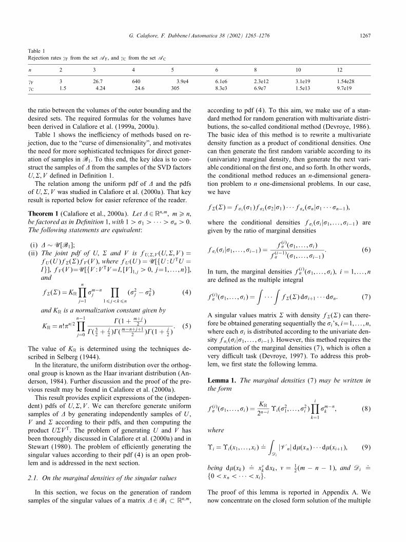
Table 1Rejection rates �F from the set AF, and �C from the set AC

n 2 3 4 5 6 8 10 12

�F 3 26.7 640 3.9e4 6.1e6 2.3e12 3.1e19 1.54e28�C 1.5 4.24 24.6 305 8.3e3 6.9e7 1.5e13 9.7e19

the ratio between the volumes of the outer bounding and thedesired sets. The required formulas for the volumes havebeen derived in Cala&ore et al. (1999a, 2000a).Table 1 shows the ine4ciency of methods based on re-

jection, due to the “curse of dimensionality”, and motivatesthe need for more sophisticated techniques for direct gener-ation of samples in B1. To this end, the key idea is to con-struct the samples of � from the samples of the SVD factorsU;�; V de&ned in De&nition 1.The relation among the uniform pdf of � and the pdfs

of U;�; V was studied in Cala&ore et al. (2000a). That keyresult is reported below for easier reference of the reader.

Theorem 1 (Cala&ore et al., 2000a). Let �∈Rn;m; m¿ n;be factored as in De)nition 1; with 1¿ 1 ¿ · · ·¿ n ¿ 0.The following statements are equivalent:

(i) � ∼ U[B1];(ii) The joint pdf of U; � and V is fU;�;V (U;�; V ) =

fU (U )f�(�)fV (V ); where fU (U ) =U[{U :UTU =I}]; fV (V )=U[{V :V TV=I; [V ]1; j ¿ 0; j=1; : : : ; n}];and

f�(�) = KRn∏

j=1

m−nj

∏16j¡k6n

( 2j − 2

k) (4)

and KR is a normalization constant given by

KR = n!�n=2n−1∏j=0

�(1 + m+j2 )

�( 32 +j2 )�(

m−n+j+12 )�(1 + j

2 ): (5)

The value of KR is determined using the techniques de-scribed in Selberg (1944).In the literature, the uniform distribution over the orthog-

onal group is known as the Haar invariant distribution (An-derson, 1984). Further discussion and the proof of the pre-vious result may be found in Cala&ore et al. (2000a).This result provides explicit expressions of the (indepen-

dent) pdfs of U;�; V . We can therefore generate uniformsamples of � by generating independently samples of U ,V and � according to their pdfs, and then computing theproduct U�V T. The problem of generating U and V hasbeen thoroughly discussed in Cala&ore et al. (2000a) and inStewart (1980). The problem of e4ciently generating thesingular values according to their pdf (4) is an open prob-lem and is addressed in the next section.

2.1. On the marginal densities of the singular values

In this section, we focus on the generation of randomsamples of the singular values of a matrix �∈B1 ⊂ Rn;m;

according to pdf (4). To this aim, we make use of a stan-dard method for random generation with multivariate distri-butions, the so-called conditional method (Devroye, 1986).The basic idea of this method is to rewrite a multivariatedensity function as a product of conditional densities. Onecan then generate the &rst random variable according to its(univariate) marginal density, then generate the next vari-able conditional on the &rst one, and so forth. In other words,the conditional method reduces an n-dimensional genera-tion problem to n one-dimensional problems. In our case,we have

f�(�) = f 1 ( 1)f 2 ( 2| 1) · · ·f n( n| 1 · · · n−1);

where the conditional densities f i( i| 1; : : : ; i−1) aregiven by the ratio of marginal densities

f i( i| 1; : : : ; i−1) =f(i)

( 1; : : : ; i)

f(i−1) ( 1; : : : ; i−1)

: (6)

In turn, the marginal densities f(i) ( 1; : : : ; i); i = 1; : : : ; n

are de&ned as the multiple integral

f(i) ( 1; : : : ; i) =

∫· · ·

∫f�(�) d i+1 · · · d n: (7)

A singular values matrix � with density f�(�) can there-fore be obtained generating sequentially the i’s, i=1; : : : ; n,where each i is distributed according to the univariate den-sity f i( i| 1; : : : ; i−1). However, this method requires thecomputation of the marginal densities (7), which is often avery di4cult task (Devroye, 1997). To address this prob-lem, we &rst state the following lemma.

Lemma 1. The marginal densities (7) may be written inthe form

f(i) ( 1; : : : ; i) =

KR2n−i Wi( 2

1 ; : : : ; 2i )

i∏k=1

m−nk ; (8)

where

Wi =Wi(x1; : : : ; xi):=∫Di

|Vn| d�(xn) · · · d�(xi+1); (9)

being d�(xk):= x k dxk ; = 1

2(m − n − 1); and Di:=

{0¡xn ¡ · · ·¡xi}.

The proof of this lemma is reported in Appendix A. Wenow concentrate on the closed form solution of the multiple


integral (9). The following key theorem provides a directway to compute the conditional densities that are needed forthe application of the conditional method.

Theorem 2. For i=1; : : : ; n; the multiple integral in (9) canbe computed as

Wi = x!ii det1=2

M (xi)Vi−1

0

−VTi−1 0 0

; (10)

where the blocks corresponding to the term Vi−1 =Vi−1(x1; : : : ; xi−1) are not present if i = 1; and !i

:=( + 1)(n− i);

M (xi):=

[OS(xi) X(xi)

−XT(xi) 0

]if (n− i) even;

OS(xi) X(xi) OF(xi)

−XT(xi) 0 0

− OFT(xi) 0 0

if (n− i) odd;

(11)

and; for r; j = 1; : : : ; n;

OSrj(xi):=

r − j(r + )(j + )(r + j + 2 )

xr+j−2i ;

OFj(xi):=

x j−1i

j + ; Xj(xi)

:= x j−1i :

(12)

The proof of this result is lengthy and requires the introduc-tion of further preliminary concepts. The complete proof isreported in Appendix C.

Remark 1. Notice that the matrix appearing in (10) is askew-symmetric polynomial matrix of even order; thereforeits determinant is always a perfect square in the entries ofthe matrix; see e.g. Vein and Dale (1999). Considering thefactor x!ii in (10); and recalling that = (m− n− 1)=2; it isstraightforward to verify that Wi( 2

1 ; : : : ; 2i ) is a multivariate

polynomial in 1; : : : ; i. At the ith step of the conditionalmethod; the variables 1; : : : ; i−1 are assigned to numericalvalues; therefore the conditional density f i( i| 1; : : : ; i−1)de&ned in (6) is a univariate polynomial in i. Sample gen-eration according to a given univariate polynomial densityis a standard problem; and can be e4ciently performed us-ing one of the available methods; see e.g. Devroye (1986).

2.2. An e;cient algorithm for the generation of thesingular values

In this section, we propose an e4cient algorithm for com-puting recursively the marginal densities given in (8), us-ing the results of Theorem 2. We &rst state a lemma that

provides a direct way to compute the square root of the de-terminant of real skew-symmetric matrices obtained addingtwo rows and two columns to a given real skew-symmetricmatrix of even order. Formally, let q be an even integer and,for k = 1; : : : ; q=2, let OH 2k(x)∈Rq+2(k−1);2 be a polynomialmatrix in the scalar variable x, with

OH 2k(x):=

[H2k(x)

02(k−1);2

]; H2k(x)

:= [h2k−1(x) h2k(x)];

(13)

where h2k−1(x); h2k(x)∈Rq;1 are given polynomial vectorsin x. Let also Q0(x)∈Sq be a given skew-symmetric poly-nomial matrix, and de&ne, for k = 1; : : : ; q=2, the borderedmatrix

Q2k(x):=

[Q2(k−1)(x) OH 2k(x)

− OHT2k(x) 02;2

]∈Sq+2k (14)

and, for k = 0; : : : ; q=2,

p2k(x):=√|Q2k(x)|: (15)

Notice that, from the properties of determinants ofskew-symmetric matrices it follows that p2k(x) is a poly-nomial in x, see for instance Vein and Dale (1999). Weare now ready to state the following lemma, which playsa key role for the development of the sample generationalgorithm.

Lemma 2. The polynomial p2k(x) de)ned in (15) may becomputed (up to a sign) as

p2k(x) =± d2k(x)

p2k−10 (x)

for k = 1; : : : ; q=2; (16)

where p0(x) =√|Q0(x)|; and d2k(x) is a polynomial

determined according to the following recursion: fork = 1; : : : ; q=2;

d2k(x) = hT2k−1(x)Z2(k−1)(x)h2k(x); (17)

Z2k(x) = d2k(x)Z2(k−1)(x)+Z2(k−1)(x)(H2k(x)JH2k(x)T)Z2(k−1)(x); (18)

where Z0(x) = AdjQ0(x);

J :=

[0 1

−1 0

]

and H2k ; h2k−1; h2k are de)ned in (13).

The proof of this lemma is reported in Appendix B.The result of Lemma 2 is now used to develop an e4cient

recursive algorithm for the generation of the singular values.In order to apply Lemma 2 to the result of Theorem 2, fourdiMerent cases need to be considered, corresponding to thecombinations of n and i being even or odd. This is necessary


since Lemma 2 requires the use of matrices of even order.We explain the use of the lemma for the case n even, thecase n odd follows from a similar reasoning. Consider thecase n even: we construct two parallel recursions, one thatholds for i even, and one for i odd. If i is even, then thedeterminant in (10) may be immediately rewritten in form(14), with i = 2k,

Q0(xi) = OS(xi); H2k = [X (x2k−1) X (x2k)]:

Thus, recursion (17) provides the Wi’s for i even. If i isodd, then the determinant in (10) may still be rewritten inthe form of Lemma 2, shifting the indices k ← k + 1=2in (14)

Q1(xi) =

OS(xi) OF(xi) X(xi)

− OFT(xi) 0 0

−XT(xi) 0 0

;

H2k+1 =

X (x2k) X (x2k+1)

0 0

0 0

:

Recursion (17) now provides the Wi’s for i odd.We report below the algorithm for the generation of the

singular values. In the algorithm, we denote with x and thecurrent variables, while the subscripted terms xi; i denotevariables evaluated to their numerical values.

Algorithm. De)ne the following quantities:

Q(e)0 (x) = OS(x); Q(e)

1 (x) =

OS(x) OF(x) X(x)

− OFT(x) 0 0

−XT(x) 0 0

;

Q(o)0 (x) =

[ OS(x) OF(x)

− OFT(x) 0

]; Q(o)

1 (x) =

[OS(x) X(x)

−XT(x) 0

];

where OS; OF; and X are de)ned in (12). A random matrix�=diag( 1; 2; : : : ; n) distributed according to (4); can begenerated via the following algorithm.

Initialization (see Remark 2).

• If n is even, then

Z0(x) = AdjQ(e)0 (x); Z1(x) = AdjQ(e)

1 (x)

p0(x) =√|Q(e)

0 (x)|; p1(x) =√|Q(e)

1 (x)|:

• If n is odd, then

Z0(x) = AdjQ(o)0 (x); Z1(x) = AdjQ(o)

1 (x)

p0(x) =√|Q(o)

0 (x)|; p1(x) =√|Q(o)

1 (x)|:

• W1(x) = x( +1)(n−1)p1(x).• f(1)

( ) = KR=(2n−1)W1( 2) m−n.• Generate 1 according to f 1 ( ) ≡ f(1)

( ). Set x1 = 21.

• k = 1, if n= 1 then go to [End].

Generation (even).

• If n even, h(x) =X(x), else h(x) =[X(x)0

].

• d2k(x) = hT(x2k−1)Z2(k−1)(x)h(x).

• p2k(x) = d2k(x)=p2k−10 (x).

• W2k(x) = W2k( 21 ; : : : ;

22k−1; x) = x( +1)(n−2k)p2k(x).

• f(2k) ( ) =f(2k)

( | 1; : : : ; 2k−1)

=± (KR=(2n−2k))W2k( 2) m−n2k−1∏j=1

m−nj :

• Generate 2k according to

f 2k ( ) = f(2k) ( )=f(2k−1)

( 1; : : : ; 2k−1). Set x2k = 22k .

Update (even).

• d2k(x) = hT(x2k−1)Z2(k−1)(x)h(x2k).

• Z2k(x) = d2k(x)Z2(k−1)(x) + Z2(k−1)(x)·×[h(x2k−1)h(x2k)]J [h(x2k−1)h(x2k)]TZ2(k−1)(x).

• If 2k + 1¿n, then goto [End].

Generation (odd).

• If n even, h(x) =

[X(x)

0

], else h(x) =

X(x)

0

0

.

• d2k+1(x) = hT(x2k−1)Z2k−1(x)h(x2k).

• p2k+1(x) = d2k+1(x)=p2k−11 (x).

W2k+1(x) =W2k+1( 21 ; : : : ;

22k ; x)

= x( +1)(n−2k−1)p2k+1(x):

f(2k+1) ( ) =f(2k+1)

( | 1; : : : ; 2k)

=±(KR=(2n−2k−1))W2k+1( 2) m−n

×2k∏j=1

m−nj :

• Generate 2k+1 according to

f 2k+1( ) = f(2k+1) ( )=f(2k)

( 1; : : : ; 2k). Set x2k+1 = 22k+1.

Update (odd).

• Z2k+1(x) = d2k+1(x)Z2k−1(x) + Z2k−1(x)×[h(x2k)h(x2k+1)]J [h(x2k)h(x2k+1)]TZ2k−1(x).


Loop.

• If k = �n=2� then goto [End].• k = k + 1; goto [Generation (even)].

End.

• Return �= diag( 1; : : : ; n).

Remark 2. The data required by the initialization phaseof the algorithm are simply determined as follows. De&neD(x) := diag(1; x; x2; : : : ; xn−1); 0 := (n=2)(n − 1); then wehave that Q(e)

0 (x) = D(x)Q(e)0 (1)D(x); and AdjD(x) =

diag(x0; x0−1; : : : ; x0−n+1); AdjQ(e)0 (x) = AdjD(x)AdjQ(e)

0

(1)AdjD(x). Similarly; we get AdjQ(e)1 (x)=Adj diag(D(x);

x0; x0)AdjQ(e)1 (1)Adj diag(D(x); x0; x0). Therefore; for the

even case; we have

p0(x) = x0√|Q(e)

0 (1)|; p1(x) = x0√|Q(e)

1 (1)|:

We proceed in an analogous way for the odd case;writing AdjQ(o)

0 (x)=Adj diag(D(x); x0)AdjQ(o)0 (1)Adj diag

(D(x); x0); AdjQ(o)1 (x) = Adj diag(D(x); x0)AdjQ(o)

1 (1)Adj diag(D(x); x0). Therefore; for the odd case; we have

p0(x) = x0√|Q(o)

0 (1)|; p1(x) = x0√|Q(o)

1 (1)|:

Remark 3. The sign uncertainty on the conditional densitiesis resolved in the algorithm imposing that the f(i)

’s arepositive on their domains.

Notice also that the only operations required for theconstruction of the conditional densities are simple matrixadditions and multiplications. No inversion or computationof determinants of polynomial matrices are required. Thegeneration of each i according to the resulting univariatepolynomial density may be performed very e4ciently us-ing, for instance, the methods described in Devroye (1986).The computational cost required to generate one sample of� is basically n times the cost required to generate one i.

3. A probabilistic framework for uncertain systems

In recent years, we witnessed a widespread use of algo-rithms based on uncertainty randomization, for the analysisand synthesis of robust control systems, see e.g. Ray andStengel (1993); Tempo and Dabbene (1999); Vidyasagarand Blondel (2001) and Vidyasagar (2001). The main ideabehind randomized methods is to associate a probability dis-tribution to the uncertainty set, and to assess system perfor-mance in terms of empirical probability.We brieXy recall below the basic randomized algorithms

for estimating empirical probability and the expected value,

and discuss various examples of application in the followingsections.Let � be a random variable with pdf f�(�) over the set

�� and let g(�) be a (Lebesgue) measurable function of�. The expected value of g(�) is denoted as E(g(�)). Anempirical estimate EN of E(g(�)) is given by

EN =1N

N∑i=1

g(�i);

where �i; i = 1; : : : ; N are i.i.d. samples generated accord-ing to the pdf f�(�). The estimate EN is usually referred toas the empirical mean. Given accuracy 4∈ (0; 1) and con)-dence �∈ (0; 1), if

N¿log 2

�

242

samples are drawn (ChernoM, 1952), then the empiri-cal mean is close to the actual mean in probability, i.e.Prob{|E�(g(�))− EN |6 4}¿ 1− �.

It should be remarked that the sample size N given bythe ChernoM bound is independent of the size of �� andthe pdf f�(�). If the costs associated with the generationof each sample �i and the evaluation of g(�i) for &xed�i are both polynomial-time, then the estimation of theempirical mean can be performed in polynomial-time. Forfurther details on randomized algorithms, see for instanceTempo and Dabbene (1999) and Vidyasagar (1997). Sim-ilarly, the problem of estimating the probability pA that �belongs to a set A ⊆ �� is reduced to the computation ofthe empirical mean, taking as g(�) the indicator functionof A.The next sections present examples of application of the

randomized approach to a selection of problems arising insystems and control. In particular, we consider the compu-tation of the solution for uncertain least-squares problems,the probabilistic counterpart of the real structured stabilityradius, and the assessment of approximate feasibility of un-certain linear matrix inequalities (LMI). An application toreduced order controller design in an H∞ framework maybe found in Cala&ore et al. (2000b). Also, a probabilisticapproach to the stability analysis of families of paramet-ric polynomials is presented in Polyak and Shcherbakov(2000).

3.1. Uncertain least-squares problems

In this section, we consider the problem of determiningapproximate solutions to the system of linear equations

A(�)x = b(�);

where x∈Rn, b∈Rm, and A and b are generic functions(a4ne or not) of the uncertainty �∈�1 in form (1). Thesolution of this problem in a deterministic worst-case setting


is studied in Cala&ore and El Ghaoui (2001) and El Ghaouiand Lebret (1997); the worst-case solution is computed as

xRLS = argminx

max�‖A(�)x − b(�)‖2: (19)

Here, we assume instead that � is a random matrix withgiven radially symmetric probability distribution over �1,and seek a solution x such that

x = argminx

E{‖A(�)x − b(�)‖2}: (20)

To the authors knowledge, the above problem has in generalno analytical solution. In a randomized approach, we gener-ate N samples �i of the uncertainty, and look for a solutionxN such that the empirical mean is minimized

xN = argminx

EN (x);

where

EN (x):=

1N

N∑i=1

‖A(�i)x − b(�i)‖2:

The solution of the above problem is of course still in theform of an LS problem, and may be e4ciently computedrecursively. Assuming w.l.o.g. that A(�1) is full-rank, wehave

xk+1 = xk + R−1k+1A

T(�k+1)(b(�k+1)− A(�k+1)xk);

where Rk+1 =Rk +AT(�k+1)A(�k+1), and the recursion fork = 1; : : : ; N is started with R0 = 0; x0 = 0. As a numericalexample, we considered the following data, adapted from ElGhaoui and Lebret (1997),

A=

3 1 4

0 1 1

−2 5 3

1 4 5:2

; b=

0

2

1

3

;

where A(�) = A + �, with O (�)6 1. Taking N = 10; 000uniform samples of �, we obtained the solution xTN =[ − 0:1768 0:1009 0:3448]. The standard LS estimate isxLS = (ATA)−1ATb= [− 10:0 − 9:7285 9:9834]T, and therobust estimate introduced in El Ghaoui and Lebret (1997)

Table 2Statistics for comparison of residuals: average, peak, and regularity

Average Peak Sample covariance

rN 2.2650 2.6344 0.0198rLS 11.8962 18.5164 9.409rRLS 2.2848 2.5515 0.0107

is xRLS=[−0:0312 0:2073 0:2055]T. To compare the results,we computed the estimation residuals riN

:= ‖A(�i)xN −b‖; riLS

:= ‖A(�i)xLS − b‖; riRLS:= ‖A(�i)xRLS − b‖, for

a large number of uncertainty samples �i, and obtainedthe statistics reported in Table 2. Also, the worst-case(with respect to the uncertainty) residuals, de&ned asrwc∗

:= max�‖A(�)x∗ − b(�)‖, result in rwcN = 2:6532; rwcLS =18:9394; rwcRLS = 2:572.Problem (20) may therefore be e4ciently solved using

the proposed randomized approach. The resulting solutionhas, at least on the data used in the example, a performancewhich is very close to that of the deterministic worst-casecounterpart (19). It should be also remarked that (19) maybe solved exactly only in some special cases (see El Ghaoui& Lebret, 1997), while the randomized approach presentsno computational complexity issues, and works equally wellwhen the data depends in a non-linear way on the uncer-tainty, and when the uncertainty has a more complicatedblock structure.

3.2. The probabilistic structured real stability radius

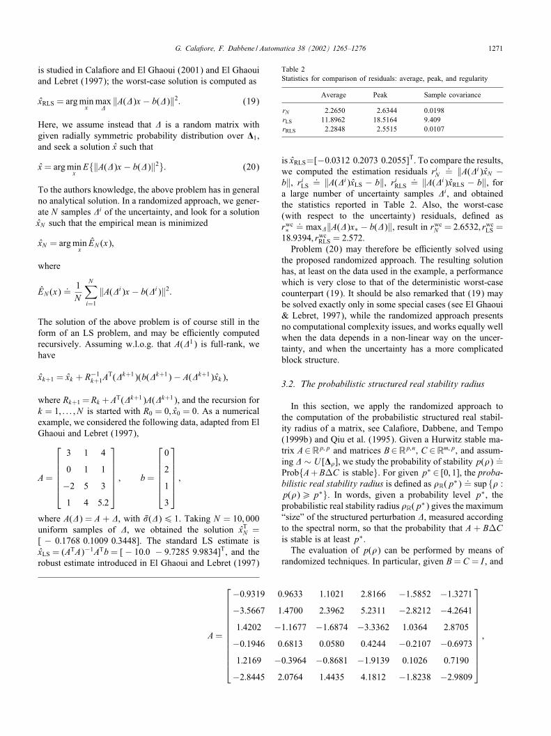
In this section, we apply the randomized approach tothe computation of the probabilistic structured real stabil-ity radius of a matrix, see Cala&ore, Dabbene, and Tempo(1999b) and Qiu et al. (1995). Given a Hurwitz stable ma-trix A∈Rp;p and matrices B∈Rp;n, C ∈Rm;p, and assum-ing � ∼ U [��], we study the probability of stability p(�) :=Prob{A+BZC is stable}. For given p∗ ∈ [0; 1], the proba-bilistic real stability radius is de&ned as �R(p∗) := sup {� :p(�)¿p∗}. In words, given a probability level p∗, theprobabilistic real stability radius �R(p∗) gives the maximum“size” of the structured perturbation �, measured accordingto the spectral norm, so that the probability that A + BZCis stable is at least p∗.The evaluation of p(�) can be performed by means of

randomized techniques. In particular, given B= C = I , and

A=

−0:9319 0:9633 1:1021 2:8166 −1:5852 −1:3271−3:5667 1:4700 2:3962 5:2311 −2:8212 −4:26411:4202 −1:1677 −1:6874 −3:3362 1:0364 2:8705

−0:1946 0:6813 0:0580 0:4244 −0:2107 −0:69731:2169 −0:3964 −0:8681 −1:9139 0:1026 0:7190

−2:8445 2:0764 1:4435 4:1812 −1:8238 −2:9809

;


0.01 0.015 0.02 0.025 0.03 0.035 0.04 0.045 0.050.75

0.8

0.85

0.9

0.95

1

1.05

Uncertainty radius ρ

Pro

babi

lity

of s

tabi

lity

Fig. 1. Estimated probability of stability. The solid line shows the resultsobtained with a perturbation structure of three 2 × 2 blocks; the dottedline shows the results obtained with a perturbation structure of a 4 × 4and a 2× 2 blocks.

we considered two diMerent perturbation structures, one with� composed of three 2× 2 full real blocks, and one with �composed of a 4×4 and a 2×2 full real blocks. Fig. 1 showsthe degradation of the empirical probability of stability, asthe perturbation radius � varies between 0:01 and 0:05.

3.3. Approximate feasibility of uncertain LMIs

An uncertain LMI constraint is a convex constraint in thevector variable �∈Rm of the form

F(�; �) ≺ 0; �∈��; (21)

where ‘≺’ means “negative de&nite”, and F(�; �)=F0(�)+∑mi=1 �iFi(�), with Fi = FT

i . A given vector � is said to berobustly feasible for (21) if it satis&es (21) for all �∈��. Alarge number of problems arising in robust control may becast as feasibility problems involving uncertain LMIs of thetype above, see (Boyd, El Ghaoui, Feron, & Balakrishnan,1994; El Ghaoui et al., 1998). A classical example is forinstance the assessment of quadratic stability of an intervalmatrix, Boyd et al. (1994). Robust semide&nite program-ming (SDP) theory (Ben-Tal et al., 2000; El Ghaoui et al.,1998) develops computable su4cient conditions for robustfeasibility of uncertain LMIs.Given a candidate solution �, we here consider the

problem of assessing the probability p of satisfaction of(21). The solution � will be called a p-approximately feasi-ble solution for (21), see also Cala&ore and Polyak (2001).To this end, de&ne the sets

�good:= {�∈�� : F(�; �) ≺ 0};

�bad:= {�∈��:� �∈ �good}:

Assuming uniform density over ��, we have

p(�) := Prob{F(�; �) ≺ 0}=Vol{�good}:

We then use the randomization procedure to compute anempirical estimate pN of p. This approach has been usedfor design and analysis of robust LMIs in Cala&ore andPolyak (2001), to which the reader is referred for numericalexamples.

4. Conclusions

Deterministic worst-case analysis and synthesis methodsfor uncertain systems are, by and large, based on a struc-tured description of the uncertainty, which is restricted in aspectral (operator) norm bounded set. To compare consis-tently deterministic results with the recently emerged prob-abilistic ones, a technique to e4ciently generate uncertaintysamples uniformly distributed in the above set turned out tobe fundamental. This was the main technical issue discussedin this paper.The proposed sample generation technique relies on the

result of Theorem 1 for the closed form expression of themarginal probability densities of the singular values of uni-form matrices, and on an e4cient recursive implementationof the conditional method for their actual generation.The use of the proposed framework has then been illus-

trated, presenting several applications to the solution of hardproblems arising in the systems and control area.

Acknowledgements

This paper has bene&ted from useful discussions and valu-able inputs from several people. The authors express grat-itude to Laurent El Ghaoui, Augusto Ferrante and FulvioRicci. A special thanks goes to Roberto Tempo for its pre-cious help in revising the manuscript, and to an anonymousreviewer for pointing out the interesting set inclusion usedin Section 2.

Appendix A. Proof of Lemma 1

Consider (4), and introduce the change of variables xk = 2k ; k = 1; : : : ; n. Then the Jacobian of the transformation

from x to is 1=(2n∏

k√xk) (see for instance, Devroye,

1986 for the rule of change of variables in probability densityfunctions), and the pdf in the new variables is expressed as

fx(x1; : : : ; xn) =KR2n

∏16j¡k6n

(xj − xk)n∏

k=1

x k ; (A.1)

where 1¿x1 ¿x2 ¿ · · ·¿xn ¿ 0, and := (m− n− 1)=2.Notice that fx can be written in terms of the determinant ofa Vandermonde matrix Vn

fx(x1; : : : ; xn) =KR2n|Vn(x1; : : : ; xn)|

n∏k=1

x k : (A.2)


The marginal densities of x can be then written as

f(i)x (x1; : : : ; xi) =

KR2n

Wi(x1; : : : ; xi)i∏

k=1

x k ; (A.3)

where Wi:=

∫Di|Vn| d�(xn) · · · d�(xi+1), and d�(xk)

:=x k dxk ; Di

:= {0¡xn ¡ · · ·¡xi}. Statement (8) can bedirectly obtained from (A.3), applying again the change ofvariable rule.

Appendix B. Proof of Lemma 2

For k = 1; : : : ; q=2, de&ne Z2k ∈Sq as

Z2k =[Iq 0q;2k

]Q−1

2k

[Iq

02k;q

]: (B.1)

De&ne D2k ∈S2 as D2k = OHT2kQ

−12(k−1)

OH 2k , then, in view of(13) and (B.1), we have that

D2k = HT2k Z2(k−1)H2k =

[0 d(x)

−d(x) 0

];

where d2k(x) = hT2k−1Z2(k−1)h2k is a scalar function of x.We are interested in computing p2k(x) =

√|Q2k(x)|.Consider then (14) and apply the Schur rule for determi-nants, obtaining |Q2k(x)| = |Q2(k−1)| · |HT

2kQ−12(k−1)H2k | =

|Q2(k−1)| · |D2k |. Then p22k(x) = p2

2(k−1)(x)d22k(x). Notice

that to compute d2k we need Z2(k−1), which can be com-puted recursively. To this aim, we &rst compute the in-verse of Q2k , using the block matrix inversion rule. Setting9 := Q−1

2(k−1)OH 2k D

−12k , we have

Q−12k =

Q−1

2(k−1) − 9 OHT2kQ

−12(k−1) −9

9T D−12k

:

Using (B.1) it is straightforward to obtain the recursion

Z2k = Z2(k−1) +1

d2kZ2(k−1)H2kJHT

2k Z2(k−1): (B.2)

Since we are interested in a recursion involving polyno-mial matrices, we need to normalize the quantities d2k andZ2k , so to eliminate denominators. It can be shown thatthe choice d2k

:= d2kp20

∏k‘=1 d2‘; Z2k

:= Z2kp20

∏k‘=1 d2‘,

corresponding to the normalization Z0:= |Q0|Q0 = AdjQ0,

leads to the desired polynomial recursion given in (17)and (18).

Appendix C. Technical Preliminaries and Proofof Theorem 2

First, we recall that the determinant of a matrix X ∈Sn iszero if n is odd, and is a perfect square in the entries of X ifn is even. The notation X j1 ;:::; jp denotes the matrix obtainedremoving the rows and columns of indices j1; : : : ; jp from

matrix X . The notation X i1 ;:::;ip;j1 ;:::; jp denotes the matrix ob-tained removing the rows of indices i1; : : : ; ip, and columnsof indices j1; : : : ; jp from matrix X .

C.1. Preliminaries

Pfa;ans: Let S ∈Sn, then its Pfa;an is de&ned as thefollowing polynomial in the entries sij of S

Pf (S) :=1

2mm!

n∑j1 ;:::; jn=1

E(j1; : : : ; jn)sj1j2sj3j4 · · · sj2m−1j2m ;

where m = �n=2�, and E(x1; : : : ; xn) is an alternant func-tion called signature function, de&ned as E(x1; : : : ; xn)

:=∏16i¡j6n sign(xj − xi): In particular, E(x1; : : : ; xn) = 0 if

any two of the xi’s are equal. For further details on the def-inition and properties of Pfa4ans, the reader is referred toPrasolov (1994) and Weyl (1946). A fundamental propertyof the Pfa4an is that, for n even Pf 2(S) = det(S).The following result on bordered Pfa4ans will be useful

in the sequel, and may be found in Vein and Dale (1999,Chap. 4).

Lemma C.1. Let S ∈Sn with n odd; consider the borderedmatrix

S(1) =

S a1

−aT1 0

;

where aT1 = [a11 · · · an1]; then the Pfa;an of S(1) may beexpressed as Pf (S(1)) =

∑nj=1(−1) j+1aj1 Pf (Sj).

We next report an extension of the previous result, whichmay be easily proved by induction.

Lemma C.2. Let S ∈Sn and consider the bordered matrix

S(p) =

S A

−AT 0

; A=

a11 · · · a1p

... · · · ...

an1 · · · anp

;

where n + p is even. De)ning ‘(A; j1; : : : ; jp):=

(−1) j1+···+jp+pE(j1; · · · ; jp)aj1 ;1aj2 ;2 · · · ajp;p; the Pfa;anof S(p) may be expressed as

Pf (S(p)) =n∑

j1 ;:::; jp=1

‘(A; j1; : : : ; jp)Pf (Sj1 ;:::; jp):

C.1.1. A multiple integral of a determinantWe here make use of the following result regarding a

multiple integral of a special type of determinant.


Theorem C.3 (de Bruijn, 1955). Consider the integral

I(<) =∫ <

0· · ·

∫ <

0|[=(z1) (z1) · · · =(zp) (zp)]|

×d�(z1) · · · d�(zp);

where =(@); (@) are arbitrary n-dimensional (n = 2p)vector real functions of the real variable @; integrableover [0; <]; and �(@) is a suitable measure. De)ning thematrix S(<)∈Sn; whose (i; j)th element; i; j = 1; : : : ; n; isgiven by

[S(<)]i; j:=∫ <

0[=i(@) j(@)− i(@)=j(@)] d�(@); (C.1)

we have that I(<) = p! Pf (S(<)).

Below, we provide an extension of de Bruijn’s theorem thatplays a key role for our subsequent developments.

Theorem C.4. Consider the integral

I(<) =∫ <

0· · ·

∫ <

0|[A =(z1) (z1) · · · =(zp) (zp)]|

×d�(z1) · · · d�(zp); (C.2)

where A∈Rn; r ; 2p + r = n; and =(@); (@) are arbitraryn-dimensional vector real functions of the real variable z;integrable over [0; <]; and �(@) is a suitable measure. De)nethe matrix S(p)(<)∈Sn+p as

S(p)(<) :=

S(<) A

−AT 0

;

where S(<)∈Sn is de)ned as in (C.1). Then

I(<) = p! Pf (S(p)(<)): (C.3)

Proof. De&ne A = A(z1; : : : ; zp):= [A =(z1) (z1) · · ·

=(zp) (zp)]. We &rst expand the determinant in (C.2) withrespect to the columns of A; using the Laplace expansion(Vein & Dale; 1999);

|A|=n∑

j1 ;:::; jp=1

‘(A; j1; : : : ; jp)|Aj1 ;:::; jp;1;:::;p|: (C.4)

Integrating (C.4) we obtain

I(<) =n∑

j1 ;:::; jp=1

‘(A; j1; : : : ; jp)∫ <

0· · ·

∫ <

0|Aj1 ;:::; jp;1;:::;p|

×d�(z1) · · · d�(zp):

The integrals appearing in the above expression may becomputed using Theorem 3; obtaining∫ <

0· · ·

∫ <

0|Aj1 ;:::; jp;1;:::;p| d�(z1) · · · d�(zp) = p! Pf (Z(<));

where Z(<) also depends on the indices (j1; : : : ; jp); andmay be recognized to be a principal submatrix of theskew-symmetric matrix S(<) de&ned in (C.1); that isZ(<) ≡ Sj1 ;:::; jp(<). Integral (C.2) can therefore be written as

I(<) = p!n∑

j1 ;:::; jp=1

‘(A; j1; : : : ; jp) Pf (Sj1 ;:::; jp(<)): (C.5)

The proof then follows applying Lemma C.2 to (C.5).

C.2. Proof of Theorem 2

To prove the theorem we need to consider two separatecases, depending on whether n− i is even or odd.Case n− i even: Notice &rst that in the integral (9), each

column of Vn(x1; : : : ; xn) is function of only one variable.We can therefore integrate using the method of integrationover alternate variables (Mehta, 1991). First, we integratexn; xn−2; : : : ; xi+2 over their respective domains: let F(z) :=∫ z0 X(�) d�(�), then

Wi =∫Di

|[Vi X(xi+1) F(xi+1)− F(xi+3) X(xi+3)

F(xi+3)− F(xi+5) · · · X(xn−1) F(xn−1)]|×d�(xn−1) · · · d�(xi+5) d�(xi+3) d�(xi+1):

The addition of one column to another column does notchange the determinant of a matrix, therefore

Wi =∫Di

|[Vi X(xi+1) F(xi+1) · · · X(xn−1) F(xn−1)]|

×d�(xn−1) d�(xn−3) · · · d�(xi+1): (C.6)

Notice now that the integrand in (C.6) is symmetric in theremaining variables 1 xi+1; xi+3; : : : ; xn−1, therefore one canintegrate over them independently (see Mehta, 1991) anddivide the result by ((n− i)=2)!, obtaining

Wi =(n− i2

!)−1 ∫ xi

0· · ·

∫ xi

0|[Vi X(xi+1) F(xi+1) · · ·

X(xn−1) F(xn−1)]| d�(xn−1) d�(xn−3) · · · d�(xi+1):

We can now apply the result of Theorem C.3 to the aboveintegral, obtaining

Wi(x1; : : : ; xi) = Pf

S(xi) Vi

−VTi 0

; (C.7)

1 The integrand is symmetric in the variables, since interchanging xiand xj amounts to the interchanging of two pairs of columns.


where S(xi)∈Sn is de&ned as in (C.1), with =k(x):=

Xk(x) = xk−1, and k(x):= Fk(x) =

∫ x0 �k−1� d� = (xk+ =

(k + )), for k = 1; : : : ; n. Therefore,

Srj(xi) =r − j

(r + )(j + )(r + j + 2 )xr+j+2 i :

De&ne now OS(xi) as in (12), such that S(xi) = x2( +1)i

OS(xi).Then, recalling that Vi =[Vi−1 Xi], and that the exchangeof one row and one column does not aMect the determinant,factoring out the term x2( +1)

i from the Pfa4an, we rewrite(C.7) as

Wi = x( +1)(n−i)i Pf

OS(xi) X(xi) Vi−1

−XT(xi) 0 0

−VTi−1 0 0

; (C.8)

from which follows the statement of (11).Case n − i odd. We now &rst integrate xn; xn−2; : : : ; xi+1

over their respective domains, obtaining

Wi =∫Di

|[Vi F(xi)− F(xi+2) X(xi+2)

F(xi+2)− F(xi+4) · · · X(xn−1) F(xn−1)]|×d�(xn−1) · · · d�(xi+4) d�(xi+2):

Again, performing elementary operations on the columns,we obtain

Wi =∫Di

|[Vi F(xi) X(xi+2) F(xi+2) · · · X(xn−1)

F(xn−1)]| d�(xn−1) · · · d�(xi+4) d�(xi+2):

The integrand above is symmetric in the remaining variablesxi+2; xi+4 : : : ; xn−1, therefore integrating over them indepen-dently, and dividing the result by ((n − i − 1)=2)! (Mehta,1991), we obtain

Wi =(n− i − 1

2!)−1 ∫ xi

0· · ·

∫ xi

0|[Vi F(xi)

X(xi+2)F(xi+2) · · · X(xn−1) F(xn−1)]|×d�(xn−1) · · · d�(xi+4) d�(xi+2):

We can now apply the result of Theorem 3 to the aboveintegral, obtaining

Wi(x1; : : : ; xi) = Pf

S(xi) Vi F(xi)

−VTi

−FT(xi)0

; (C.9)

where S(xi)∈Sn is de&ned as in (1). De&ning now OS(xi)and OF(xi) as in (12), the result in (11) is then obtainedfollowing the same reasoning as in the even case.

References

Anderson, T. W. (1984). An introduction to multivariate statisticalanalysis. New York: Wiley.

Bai, E. W., Tempo, R., & Fu, M. (1998). Worst case properties of theuniform distribution and randomized algorithms for robustness analysis.Mathematics of Control, Signals and Systems, 11, 183–196.

Barmish, B. R., & Lagoa, C. M. (1997). The uniform distribution: Arigorous justi&cation for its use in robustness analysis Mathematicsof Control, Signals and Systems, 10, 203–222.

Ben-Tal, A., El Ghaoui, L., & Nemirovskii, A. (2000). RobustSemide&nite programming. In R. Saigal, L. Vandenberghe, &H. Wolkowicz (Eds.), Handbook of semide)nite programming.Waterloo: Kluwer Academic Publishers.

Blondel, V. D., & Tsitsiklis, J. N. (2000). A survey of computationalcomplexity results in systems and control. Automatica, 36, 1249–1274.

Boyd, S. P., El Ghaoui, L., Feron, E., & Balakrishnan, V. (1994). Linearmatrix inequalities in systems and control theory. Philadelphia, PA:SIAM Publications.

Cala&ore, G., Dabbene, F., & Tempo, R. (1999a). Radial and uniformdistributions in vector and matrix spaces for probabilistic robustness.In D. Miller, & L. Qiu (Eds.), Topics in control and its applications(pp. 17–31). London: Springer.

Cala&ore, G., Dabbene, F., & Tempo, R. (1999b). The probabilistic realstability radius. Proceedings of the 14th IFAC world congress, Vol.G, Beijing, July 1999 (pp. 395–400).

Cala&ore, G., Dabbene, F., & Tempo, R. (2000a). Randomizedalgorithms for probabilistic robustness with real and complex structureduncertainty. IEEE Transactions on Automatic Control, 45(12),2218–2235.

Cala&ore, G., Dabbene, F., & Tempo, R. (2000b). Randomized algorithmsfor reduced order H∞ controller design. Proceedings of the Americancontrol conference, Vol. 6, Chicago, June 2000 (pp. 3837–3839).

Cala&ore, G., & El Ghaoui, L. (2001). Worst case maximum likelihoodestimation in the linear model. Automatica, 37(4), 573–580.

Cala&ore, G., & Polyak, B. T. (2001). Stochastic algorithms for exactand approximate feasibility of robust LMIs. IEEE Transactions onAutomatic Control, 46(11), 1755–1759.

ChernoM, H. (1952). A measure of asymptotic e4ciency for test ofhypothesis based on the sum of observations. Annals of Mathematicsand Statistics, 23, 493–507.

de Bruijn, N. G. (1955). On some multiple integrals involvingdeterminants. Journal of the Indian Mathematical Society, 19,127–132.

Devroye, L. (1986). Non-uniform random variate generation. New York:Springer.

Devroye, L. (1997). Random variate generation for multivariateunimodal densities. ACM Transactions on Modelling and ComputerSimulations, 7, 447–477.

El Ghaoui, L., & Cala&ore, G. (2001). Robust &ltering for discrete-timesystems with bounded noise and parametric uncertainty. IEEETransactions on Automatic Control, 46(7), 1084–1089.

El Ghaoui, L., & Lebret, H. (1997). Robust solutions to least-squaresproblems with uncertain data. SIAM Journal on Matrix Analysis andApplications, 18(4), 1035–1064.

El Ghaoui, L., Oustry, F., & Lebret, H. (1998). Robust solutions touncertain semide&nite programs. SIAM Journal on Optimization,9(1), 33–52.

Khargonekar, P. P., & Tikku, A. (1996). Randomized algorithms forrobust control analysis have polynomial time complexity. Proceedingsof the 35th IEEE conference on decision and control, Vol. 3, Kobe,December 1996 (pp. 3470–3475).

Mehta, M. L. (1991). Random matrices. Boston: Academic Press.Nemirovskii, A. (1993). Several NP-hard problems arising in robust

stability analysis. Mathematics of Control, Signals and Systems, 6,99–105.


Polijak, S., & Rohn, J. (1993). Checking robust non-singularity isNP-hard. Mathematics of Control, Signals and Systems, 6, 1–9.

Polyak, B. T., & Shcherbakov, P. S. (2000). Random spherical uncertaintyin estimation and robustness. IEEE Transactions on AutomaticControl, 45(11), 2145–2150.

Prasolov, V. V. (1994). Problems and theorems in linear algebra.Providence, RI: American Mathematical Society.

Qiu, L., Bernhardsson, L. B., Rantzer, A., Davison, E. J., Young, P. M.,& Doyle, J. (1995). A formula for computation of the real stabilityradius. Automatica, 6, 879–890.

Ray, L. R., & Stengel, R. F. (1993). A Monte carlo approach to theanalysis of control system robustness. Automatica, 29, 229–236.

Selberg, A. (1944). Bemerkninger om et multiplet integral. NorskMatematisk Tidsskrift, 26, 71–78.

Stewart, G. W. (1980). The e4cient generation of random orthogonalmatrices with an application to condition estimators. SIAM Journalon Numerical Analysis, 17(3), 403–409.

Tempo, R., Bai, E. W., & Dabbene, F. (1997). Probabilistic robustnessanalysis: Explicit bounds for the minimum number of samples Systems& Control Letters, 30, 237–242.

Tempo, R., & Dabbene, F. (1999). Probabilistic robustness analysisand design of uncertain systems. In G. Picci, & D. S. Gilliam(Eds.), Dynamical systems, control, coding, computer vision—Newtrends, interfaces, and interplay, Vol. 25 (pp. 263–282). Boston:Birkhauser.

Vein, R., & Dale, P. (1999). Determinants and their applications inmathematical physics. New York: Springer.

Vidyasagar, M. (1997). A theory of learning and generalization. London:Springer.

Vidyasagar, M. (2001). Randomized algorithms for robust controllersynthesis using statistical learning theory. Automatica, 37(10),1515–1528.

Vidyasagar, M., & Blondel, V. D. (2001). Probabilistic solutions to someNP-hard matrix problems. Automatica, 37(9), 1397–1405.

Weyl, H. (1946). The classical groups, their invariants andrepresentations. Princeton, NJ: Princeton University Press.

Xie, L., Soh, Y. C., & de Souza, C. E. (1994). Robust Kalman &lteringfor uncertain discrete-time systems. IEEE Transactions on AutomaticControl, 39(6), 1310–1314.

Zhou, K., Doyle, J. C., & Glover, K. (1996). Robust and optimal control.Upper Saddle River: Prentice-Hall.

Zhu, X., Huang, Y., & Doyle, J. (1996). Soft vs. hard boundsin probabilistic robustness analysis. Proceedings of the 35thIEEE conference on decision and control. Vol. 3, Kobe, Japan(pp. 3412–3417).

Giuseppe Cala�ore was born in Torino,Italy in 1969. He received the “Laurea” de-gree in Electrical Engineering from Politec-nico di Torino in 1993, and the Doctoratedegree in Information and System Theoryfrom Politecnico di Torino, in 1997. Since1998, he is tenured Assistant Professor atDipartimento di Automatica e Informatica,Politecnico di Torino. Dr. Cala&ore heldvisiting positions at Information SystemsLaboratory, Stanford University, in 1995, atEcole Nationale Sup_erieure de Techniques

Avence_es (ENSTA), Paris, in 1998, and at the University of California atBerkeley, in 1999. His research interests are in the &eld of analysis, iden-ti&cation and control of uncertain systems, pattern analysis and robotics,convex optimization and randomized algorithms.

Fabrizio Dabbene received the Laurea de-gree in Electronic Engineering in 1995 andthe Ph.D. degree in Systems and ComputerEngineering in 1999, both from Politecnicodi Torino, Italy. In 1997, he has been Visit-ing Researcher at the Department of Electri-cal Engineering, University of Iowa. He iscurrently holding a tenured research positionat the research institute IRITI of the NationalResearch Council (CNR) of Italy Politecnicodi Torino. Dr. Dabbene also holds collabo-ration with Politecnico di Torino where he

teaches several courses in Systems and Control. His research interestsinclude robust control and identi&cation of uncertain systems, randomizedalgorithms and optimization.

A probabilistic framework for problems with real structured uncertainty in systems and control

Documents