A Primer on Latent Profile Analysis in Mplus for Applied ...

Wayne State University Wayne State University

Kinesiology, Health and Sport Studies College of Education

11-22-2019

Finding Latent Groups in Observed Data: A Primer on Latent Finding Latent Groups in Observed Data: A Primer on Latent

Profile Analysis in Mplus for Applied Researchers Profile Analysis in Mplus for Applied Researchers

Sarah L. Ferguson Rowan University

E. Whitney G. Moore Wayne State University, [email protected]

Darrell M. Hull University of North Texas

Follow this and additional works at: https://digitalcommons.wayne.edu/coe_khs

Part of the Education Commons, Kinesiology Commons, and the Sports Sciences Commons

Recommended Citation Recommended Citation Ferguson, S. L., Moore, E. W. G., & Hull, D. M. (2020). Finding latent groups in observed data: A primer on latent profile analysis in Mplus for applied researchers. International Journal of Behavioral Development, 44(5), 458-468. DOI: 10.1177/0165025419881721

This Article is brought to you for free and open access by the College of Education at DigitalCommons@WayneState. It has been accepted for inclusion in Kinesiology, Health and Sport Studies by an authorized administrator of DigitalCommons@WayneState.

http://digitalcommons.wayne.edu/

http://digitalcommons.wayne.edu/

https://digitalcommons.wayne.edu/coe_khs

https://digitalcommons.wayne.edu/coe

https://digitalcommons.wayne.edu/coe_khs?utm_source=digitalcommons.wayne.edu%2Fcoe_khs%2F80&utm_medium=PDF&utm_campaign=PDFCoverPages

http://network.bepress.com/hgg/discipline/784?utm_source=digitalcommons.wayne.edu%2Fcoe_khs%2F80&utm_medium=PDF&utm_campaign=PDFCoverPages



https://doi.org/10.1177/0165025419881721

For Peer ReviewFinding Latent Groups in Observed Data: A Primer on Latent

Profile Analysis in Mplus for Applied Researchers

Journal: International Journal of Behavioral Development

Manuscript ID JBD-2019-05-3637.R1

Manuscript Type: Methods & Measures

Keywords: latent profile analysis, latent variable modeling, teaching paper

Abstract:

The present guide provides a practical guide to conducting latent profile analysis (LPA) in the Mplus software system. This guide is intended for researchers familiar with some latent variable modeling but not LPA specifically. A general procedure for conducting LPA is provided in six steps: (a) data inspection, (b) iterative evaluation of models, (c) model fit and interpretability, (d) investigation of patterns of profiles in a retained model, (e) covariate analysis, and (f) presentation of results. A worked example is provided with syntax and results to exemplify the steps.

http://mc.manuscriptcentral.com/ijbd

International Journal of Behavioral Development

For Peer Review

FINDING LATENT GROUPS 1

Abstract

The present guide provides a practical guide to conducting latent profile analysis (LPA) in the

Mplus software system. This guide is intended for researchers familiar with some latent variable

modeling but not LPA specifically. A general procedure for conducting LPA is provided in six

steps: (a) data inspection, (b) iterative evaluation of models, (c) model fit and interpretability, (d)

investigation of patterns of profiles in a retained model, (e) covariate analysis, and (f)

presentation of results. A worked example is provided with syntax and results to exemplify the

steps.

Keywords: latent profile analysis; latent variable modeling; teaching paper

Page 1 of 54



123456789101112131415161718192021222324252627282930313233343536373839404142434445464748495051525354555657585960

For Peer Review


Finding Latent Groups in Observed Data: A Primer on Latent Profile Analysis in Mplus for

Applied Researchers

The purpose of the present paper is to provide a practical guide on the use of latent

profile analysis (LPA) in applied research studies. Use of LPA as an analysis approach has

increased over recent years and is becoming more common in applied research. However, many

applied researchers do not take formal coursework in advanced statistical analyses such as LPA

(Henson, Hull, & Williams, 2010), and may turn to the internet and research literature for

assistance with teaching themselves new statistical techniques. Online resources and supports for

LPA do exist (e.g. the Mplus manual and discussion boards, online lectures and class notes, etc.),

but a unified guide for understanding and utilizing LPA with clear steps and examples

specifically targeted for applied research does not currently appear in the literature. This paper is

therefore intended for researchers already familiar with latent variable modeling, though not

mixture modeling or LPA specifically. A general discussion of LPA will be presented followed

by a worked example using data collected from a prior research study (Author, 2018). Syntax is

also provided to conduct LPA in Mplus with a discussion of common options and additions for

this program. The paper concludes with a discussion of LPA reporting practices, highlighting the

primary information needed to report an LPA in applied research.

This work is intended predominately for applied researchers who are interested in

exploring the applicability of LPA to their own research. Students still developing their methods

and analysis expertise may also benefit from this introduction to LPA, as well as reviewers of

research needing a brief introduction to the decision points and reporting practices of LPA. It

must be noted that this is a primer on LPA and the foundational functions and processes of this

analysis. As with any general introduction to a complex analysis, a balance is sought in this

Page 2 of 54



123456789101112131415161718192021222324252627282930313233343536373839404142434445464748495051525354555657585960

For Peer Review


guide between clarity of LPA use in applied research contexts, and the complexity of potential

issues with LPA analyses related to continuing debates in the field on key decisions (e.g.

statistical power, covariate inclusion, etc.). Therefore, the more complex technical discussions

and ongoing debates in the LPA and mixture modeling literature are outside of the scope of this

work. This guide will focus on the practical decision points in LPA and suggest common

approaches to these decisions supported by current methods research, while pointing the reader

to additional sources to cover these issues in more depth.

Latent Profile Analysis

Latent profile analysis (LPA) and latent class analysis (LCA) are techniques for

recovering hidden groups in data by obtaining the probability that individuals belong to different

groups. This occurs through examination of the distributions of groups in the data and

determining if those distributions are meaningful. It might be helpful to think of these groups,

whether they are classes of people or profiles of people as unobserved latent mixture

components. Indeed, both LCA and LPA are often referred to using the broad term Mixture

Models. The distinction between LCA and LPA is the way that groups are defined on the basis of

the observed variables. In LCA, observed variables are discrete, analogous to a binomial model

(See Masyn, 2013 and Nylund-Gibson & Choi, 2018 for more information). In LPA, observed

variables are continuous, analogous to a gaussian model (Oberski, 2016). Additionally, there is

latent transition analysis (LTA), which is any model that includes two or more latent class or

profile constructs; these constructs can be informed by different indicators or the same indicators

measured at different timepoints as a longitudinal extension (for a worked example, see Nylund-

Gibson, Grimm, Quirk, & Furlong, 2014).

LPA, and the closely associated latent class analysis, are person-oriented approaches to

Page 3 of 54



123456789101112131415161718192021222324252627282930313233343536373839404142434445464748495051525354555657585960

For Peer Review


latent variable analysis in the same family of methods as cluster analysis and mixture modeling

(Bergman & Magnusson, 1997; Bergman, Magnusson, & El-Khouri, 2003; Collins & Lanza,

2010; Gibson, 1959; Masyn, 2013; Sterba, 2013). Researchers new to LPA may benefit from a

comparison to factor analysis methods, such as confirmatory factor analysis (CFA), as LPA also

uses covariance matrices to explore relationships between observed data and latent variables

(Bauer & Curran, 2004; Bergman & Magnusson, 1997; Bergman, et al., 2003; Marsh, Lüdtke,

Trautwein, & Morin, 2009; Masyn, 2013). However, where CFA uses a covariance matrix of

items to uncover latent constructs, LPA uses a matrix of individuals to uncover latent groups of

people. The main difference is “the common factor model decomposes the covariances to

highlight relationships among variables, whereas the latent profile model decomposes the

covariances to highlight relationships among individuals” (Bauer & Curran, 2004, p. 6).

The person-oriented approach in LPA is grounded in three arguments. First, individual

differences are present and important within an effect or phenomenon. Second, these differences

occur in a logical way, which can be examined through patterns. Third, a small number of

patterns (profiles in LPA) are meaningful and occur across individuals (Bergman & Magnusson,

1997; Bergman, et al., 2003; Sterba, 2013). LPA is particularly useful for researchers in social

sciences as patterns of shared behavior between and within samples may be missed when

researchers conduct inter-individual, variable-centered analyses. For instance, if the LPA results

in three profiles are relatively evenly spread across the sample, it is easy to miss the possibly

meaningful differences between the profiles. LPA provides the opportunity to examine these

profiles and what predicts or is predicted by membership within the different profiles. Variable-

centered analyses assume the individuals within the sample all belong to a single profile or

population with no differentiation between latent subgroups.

Page 4 of 54



123456789101112131415161718192021222324252627282930313233343536373839404142434445464748495051525354555657585960

For Peer Review


LPA is undertaken in multiple steps, similar to structural equation modeling (SEM)

analyses. In SEM, for instance, researchers will typically fit a conceptual model, check the

measurement model to support their data, fit a series of structural models to identify the best fit

of their data to their theoretical models (Bauer & Curran, 2004; Kline, 2011). For LPA, the

process is similar in that the researcher works through an iterative modeling process to identify

the number of profiles to retain, fits a covariate model to explore the impact of these profiles on

other variables in the study or predict profile membership (Masyn, 2013; Sterba, 2013). If the

researcher also has a categorical grouping variable that they want to compare the profile

structures across, they can conduct a multi-group LPA, including measurement invariance

(Morin, Meyer, Creusier, & Bietry, 2016). Researchers can also test for measurement invariance

by covariate predictors by extending upon Masyn’s (2017) description of measurement

invariance testing for differential item functioning by covariates when conducting LCA models.

The overall goal of LPA is to uncover latent profiles or groups (k) of individuals (i) who

share a meaningful and interpretable pattern of responses on the measures of interest (j)

(Bergman, et al., 2003; Marsh, et al., 2009; Masyn, 2013; Sterba, 2013). This is done using joint

and marginal probabilities in within-class and between-class models. Two equations define the

within-class model:

(1)𝑦𝑖𝑗 = 𝜇(𝑘)𝑗 + 𝜀𝑖𝑗

(2)𝜀𝑖𝑗~𝑁(0, 𝜎2(𝑘)𝑗 )

where is the model implied mean and is the model implied variance, which will vary 𝜇(𝑘)𝑗 𝜎2(𝑘)

𝑗

across j = 1…J outcomes and k = 1…K classes or profiles. The general assumptions of LPA

include that outcome variables are normally distributed within each class and these within-class

outcomes are locally independent (Sterba, 2013). The between-class model represents the

Page 5 of 54



123456789101112131415161718192021222324252627282930313233343536373839404142434445464748495051525354555657585960

For Peer Review


probability of membership in a given class k:

(3)𝑝(𝑐𝑖 = 𝑘) = exp (𝜔(𝑘))/∑𝐾𝑘 = 1exp (𝜔(𝑘))

where is a multinomial intercept (fixed at 0 for the final class) and ci is the latent 𝜔(𝑘)

classification variable for the individual. The within-class and between-class models can

therefore be combined into a single model using the law of total probability resulting in:

(4)𝑓(𝒚𝑖) = ∑𝐾𝑘 = 1𝑝(𝑐𝑖 = 𝑘)𝑓(𝒚𝑖|𝑐𝑖 = 𝑘)

which is the marginal probability density function for an individual (i) after summing across the

joint within-class density probabilities for the J outcome variables, weighted by the probability

of class or profile membership from equation 3. Finally, the LPA analysis results in a posterior

probability for each individual defined as:

, (5)𝑡𝑖𝑘 = 𝑝(𝑐𝑖 = 𝑘│𝒚𝑖) =𝑝(𝑐𝑖 = 𝑘)𝑓(𝒚𝑖|𝑐𝑖 = 𝑘)

𝑓𝒚𝑖

representing the probability of an individual (i) being assigned membership (ci) in a specific

class or profile (k) given their scores on the outcome variables in the yi vector. A posterior

probability (t) is calculated for each individual in each profile, with values closer to 1.0

indicating a higher probability of membership in a specific profile. The more distinction between

the posterior probabilities for an individual, the more certainty there is around their membership

assignment (Sterba, 2013).

Model Retention Decisions

As LPA is a model testing process, multiple models are fit with varying levels of classes

or profiles. The number of models to test depends on the research topic; often published LPA

studies have found the best fitting model theoretically and statistically after comparing five to six

models (Masyn, 2013; Tein, Coxe, & Cham, 2013). Each model is then compared against the

previous model or models to make a decision regarding the number of latent profiles in the data

Page 6 of 54



123456789101112131415161718192021222324252627282930313233343536373839404142434445464748495051525354555657585960

For Peer Review


(Christie & Masyn, 2008; Marsh, et al., 2009; Masyn, 2013). Commonly, decisions regarding

model retention in LPA use Bayesian Information Criterion (BIC), Sample-Adjusted BIC

(SABIC), and Akaike’s Information Criterion (AIC) (Celeux & Soromenho, 1996; Marsh, et al.,

2009; Masyn, 2013; Tein, et al., 2013). BIC is used for model selection decisions with a lower

BIC value representing the preferred model:

(6)BIC(𝐾) = ― 2𝐿(𝐾) +𝑣(𝐾)ln 𝑛

with v(K) representing the number of parameters to be estimated in the model. The BIC can be

conservative, but it prefers parsimony in a model and has been shown to outperform other

indices with more continuous indicators (Morgan, 2014; Nylund, Asparouhov, & Muthén, 2007).

An alternative is the SABIC, which adjusts the formula to account for n and is less punitive on

the number of parameters in the model (Tein, et al., 2013). SABIC has been supported as the

most accurate information criteria index in simulation studies, particularly with smaller samples

and low class separation (Kim, 2014; Morgan, 2014):

(7)SABIC(𝐾) = ― 2𝐿(𝐾) +𝑣(𝐾)ln 𝑛 ∗ ((𝑛 + 2)/24)

Finally, AIC is an inconsistent model fit measure as it does not have strong parsimony

constraints, leading to more variation in the AIC values between models. Like BIC, lower values

of AIC indicate better model fit. AIC is calculated as:

(8)AIC(𝐾) = ― 2𝐿(𝐾) +2𝑣(𝐾)

With BIC, SABIC, and AIC, it should be noted that while lower values indicate better fit,

lower is relative (Masyn, 2013). Therefore, attention should be given to the magnitude of

difference. Consider two very different models, both of which are being examined for goodness

of fit by evaluating the relative improvement produced by a 2-class structure to a 3-class

structure. If one observes a reduction in BIC values from 18,000 to 17,950 for Example A, and a

Page 7 of 54



123456789101112131415161718192021222324252627282930313233343536373839404142434445464748495051525354555657585960

For Peer Review


reduction from 800 to 750 for Example B, the absolute difference of 50 points is not equivalent

for both models. The relative difference from 18,000 to 17,950 is smaller than the relative

difference of 800 to 750, and therefore the change for Example A might suggest equivalency

where the change for Example B might suggest a meaningful difference. Researchers need to

take the context into consideration when evaluating change between models, as there is no rule

on what level of change in fit values is considered “meaningful” across the board.

Entropy, a measure of classification uncertainty, is less common as a model retention

index due to lack of support in simulation studies (Masyn, 2013; Tein, et al., 2013). However,

entropy as a statistical measure of uncertainty can still be useful in supporting LPA model

retention as high entropy may indicate more classification uncertainty. Entropy is calculated as:

(9)E(𝐾) = ∑𝐾𝑘 = 1

∑𝑛𝑖 = 1𝑡𝑖𝑘ln 𝑡𝑖𝑘

where tik represents the posterior probabilities as shown in equation 5. Entropy is, therefore, a

measure of how well each LPA model partitions the data into profiles (Celeux & Soromenho,

1996). Entropy can range from 0 to 1 with higher values representing better fit of the profiles to

the data (Tein, et al., 2013). Note that this interpretation is somewhat counter-intuitive, as lower

entropy values actually represent more uncertainty or chaos in the model, which is akin to saying

lower values on the entropy statistic indicate more entropy (i.e. more classification uncertainty).

Values of .80 or greater provide supporting evidence that profile classification of individuals in

the model occurs with minimal uncertainty (Celeux & Soromenho, 1996; Tein, et al., 2013).

Additionally, the Lo, Mendell, and Rubin (LMR) test is sometimes used to compare

models, in a similar fashion to the χ2 difference test in other model testing analyses (Lo, Mendell,

& Rubin, 2001; Marsh, et al., 2009; Masyn, 2013; Tein, et al., 2013). LMR tests the likelihood

ratio of one model as compared to another with an adjusted asymptotic distribution instead of a

Page 8 of 54



123456789101112131415161718192021222324252627282930313233343536373839404142434445464748495051525354555657585960

For Peer Review


χ2 distribution (Lo, et al., 2001). As with the chi-square difference test, the LMR test is assessed

for significance across difference in degrees of freedom. It is interpreted with a significance test

in which statistical significance indicates the more parsimonious model (fewer profiles)

represents the relationships present in the data significantly worse than the less parsimonious

model (more profiles). In other words, the LMR test assists in determining when additional

profiles are not improving fit or discrimination of the model. Thus, a non-significant LMR test

suggests that the more parsimonious model is the better fitting and representative model.

Alternatively, the bootstrap likelihood ratio test (BLRT) can be used to evaluate the fit of

one model compared to a model with one less profile (k-1). BLRT uses parameter estimation

methods to create multiple bootstrap samples to represent the sampling distribution (Masyn,

2013; McLachlan, 1987). A statistically significant BLRT indicates the current model is a better

fit than a model with k-1 profiles. This approach has shown favorable results in simulation

studies over the LMR test (Nylund, et al., 2007). However, both the LMR and the BLRT can

suffer from never reaching a non-significant value, as the addition of parameters can represent

more of the information contained within the data. In such a situation, it is recommended that the

log likelihood values be plotted and examined for a bend or “elbow” to determine where the

model improvement gain starts to diminish relative to the additional parameters estimated

(Masyn, 2013).

Finally, as in any model testing analysis, theoretical support should exist for the final

model retained, and patterns and profiles uncovered should be interpretable (Marsh, Hau, &

Wen, 2004; Marsh, et al., 2009; Masyn, 2013). Reliance upon theory and prior work to evaluate

the reasonableness of a model is essential to LPA to ensure the final model and underlying

profiles represent interpretable and meaningful groupings of individuals within the context of

Page 9 of 54



123456789101112131415161718192021222324252627282930313233343536373839404142434445464748495051525354555657585960

For Peer Review


prior research. While it may be possible to produce models with more profiles that produce better

fit, if this results in reduced distinction between profiles, ability to define and interpret those

profiles, or increases the likelihood of capturing on chance or common error variance (e.g.,

method variance) rather than true classification distinctions, then the model with more profiles is

not beneficial to theory, science, or practical application. Researchers should examine the

underlying profiles produced in the retained model, including examination of trend or pattern

lines of profiles, to determine when profiles may be near to one another in patterns such that

distinctness is not meaningful. Profiles or classes containing less than 5% of the sample may be

spurious, and the relevance of such profiles should be carefully considered and examined for

interpretability and substantiveness (Marsh, et al, 2009; Masyn, 2013). Empirically, the lack of

support for a small proportion profile may come from examining the results of the k + 1 model to

see if that profile “collapsed” or no longer appears in the results (Masyn, 2013). Lastly, the

number of individuals represented by a small proportion profile should be taken into account, as

a small percentage from a large sample may include sufficient individuals (n = 30-60) to support

generalizability (Vincent & Weir, 2012).

It is worth noting that good practice includes reporting different close fitting models and

providing a detailed explanation of the decision-making process in selecting the retained model.

This detail helps those attempting to replicate the existence of established profiles since the

rational and decision-making process should be re-applied when possible. For example, if prior

work suggested five profiles, but the fifth was removed as a spurious minor grouping, perhaps

subsequent examinations that reveal a fifth profile would lead to the conclusion that it was not

spurious after all. Alternatively, good fit for only four profiles would help to confirm prior

judgment about the removal of the spurious, and non-theory fitting fifth profile. Additionally,

Page 10 of 54



123456789101112131415161718192021222324252627282930313233343536373839404142434445464748495051525354555657585960

For Peer Review


class separation can be used to assist researchers in understanding the differences between the

retained profiles. A profile plot of class probabilities is one way to evaluate profile separation,

and odds ratios can be used to further evaluate the differences between profiles (Masyn, 2013).

Power and sample size requirements should also be considered for planned LPA studies.

Power analysis in LPA is a developing area in the field with promising advances (Gudicha, 2015;

Park & Yu, 2017; Tein, et al., 2013). However, there is currently no simple formula or calculator

to estimate required sample size in LPA. The required sample size is dependent on the number of

profiles and the distance between the profiles, which is unknown in advance and can only be

estimated based on prior research (Tein, et al., 2013). Across 38 studies, the median sample size

was found to be n = 377, while some simulation studies have suggested samples of 300 to 500

would qualify as a minimum sample (Finch & Bronk, 2011; Nylund, et al., 2007; Peugh & Fan,

2014; Tein, et al., 2013). Readers are referred to Preacher and Coffman (2006) and MacCallum,

Browne, and Sugawara (1996) for further information on power analysis in covariance modeling.

Covariate Analyses

Following the profile retention decision in LPA is the examination of covariates to

discover relationships and differences between latent groups (Clark & Muthen, 2009; Marsh, et

al., 2009; Nylund-Gibson & Masyn, 2016). Exploring relationships with covariates provides

additional information on the latent profiles and how the covariate variables may have differing

effects on these profiles. One key point here, as highlighted in Marsh, et al. (2009), is the

“covariates are assumed to be strictly antecedent variables” (p. 195) and have no effect on the

formation of the profiles themselves. Historically, covariates were considered antecedents and

not outcomes, because if the covariates were included in the model as outcomes, then they would

alter the definition of the latent classes when entered into the model (Nylund-Gibson & Masyn,

Page 11 of 54



123456789101112131415161718192021222324252627282930313233343536373839404142434445464748495051525354555657585960

For Peer Review


2016). Thus, latent classes were regressed on the covariates of interest, not the other way around;

which allowed for some freedom in the method of covariate inclusion, as these covariates should

not influence the LPA profile solution. When to include covariates has been debated within the

LPA/LCA literature; simulation studies have supported the preference for including covariates

after the original model retention decision is made (Nylund-Gibson & Masyn, 2016).

There are three methods of covariate inclusion in the current LPA literature. Method one

is to examine the profiles based on each individual’s most likely membership, and then explore

the relationship of the profiles with the covariates in a separate post hoc analysis. Using this

method, researchers first assign each individual to the profile for which they have the highest

posterior probability. Then, the relationship between profile groups, as defined by individuals

placed into their most likely profile, and the study covariates are evaluated. This turns the latent

profiles into a categorical grouping variable, which decreases the computational burden of other

approaches. However, this option is only recommended if entropy, or the level of classification

uncertainty in the model, is above 0.80 (Clark & Muthen, 2009). This is recommended because

profile classifications are treated as fixed, categorical variables, rather than latent profiles with

flexibility (e.g., the probability associated with them). If the entropy value is less than .80 (i.e.,

classification uncertainty in the model is increased), this approach may falsely force individuals

into profiles without clear justification. Marsh, et al. (2009) and Christie and Masyn (2010)

provide examples of this post hoc approach to covariate analysis.

Method two is a more advanced approach to LPA covariate inclusion called the ML

three-step approach, which is also sometimes referred to as the VAM approach (Asparouhov &

Muthén, 2014; Vermunt, 2010). This approach follows the same first step as method one in that

the latent profiles are evaluated first. In step two, the individuals are assigned to their most likely

Page 12 of 54



123456789101112131415161718192021222324252627282930313233343536373839404142434445464748495051525354555657585960

For Peer Review


profile using the posterior probabilities provided from the initial latent profile analysis, similar to

method one. However, the ML three-step approach approaches differs in the estimation of the

model with the covariates included, because the profile assignment uncertainty is added into the

model syntax by using the estimated average classification errors for each profile from step two.

In this way, the third method accounts for the average uncertainty in profile assignment while

modeling the effects of covariates on or with the profiles (Asparouhov & Muthén, 2014;

Vermunt, 2010). For further reading on this method, readers are pointed to Asparouhov and

Muthén (2018) and Nylund-Gibson, Grimm, and Masyn (2018).

Finally, method three is the BCH approach, also a three-step approach (Asparouhov &

Muthen, 2018; Masyn, 2013; McLarnon & O’Neill, 2018). The first step of the BCH approach is

again determining the number of latent profiles without including the covariates in the model

(Clark & Muthen, 2009; Marsh, et al., 2009). Similar to the VAM approach described above, in

the second step the participants’ individual class probabilities are used to specify their

probability of membership into each latent profile. Therefore, this method includes individual

rather than average uncertainty in profile classification. Although this makes the BCH approach

computationally complex, simulation studies have found this approach to be a relatively robust

method over method one (Clark & Muthen, 2009; Nylund-Gibson & Masyn, 2016). There are

now default commands available within Mplus for the most basic implementation of the BCH

approach (see syntax for example of how to implement these steps; for further details regarding

the limitations of the default command options in Mplus see Asparouhov & Muthen, 2018).

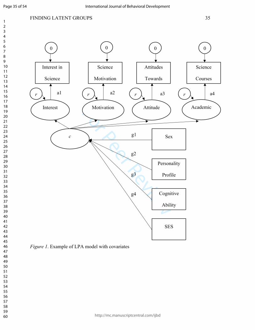
Using the BCH approach means that indicators for the profiles are present in the model with the

covariates during analysis as shown in Figure 1. Note in the figure how the latent profiles predict

responses on the indicators, while the antecedent covariates are predicting the profiles. The

Page 13 of 54



123456789101112131415161718192021222324252627282930313233343536373839404142434445464748495051525354555657585960

For Peer Review


example provided in the current article uses this approach.

The second and third methods described above are currently recommended over the post

hoc approach because they both allow for the uncertainty of profile assignment to remain in the

model while also usually being able to maintain the integrity of the profiles when the covariates

are added in. It is important to confirm that the profiles have not changed once the covariates are

added into the model, as such fluctuations may indicate the presence of differential item

functioning for one or more of the profile indicators in relation to the covariates (Masyn, 2017;

Nylund-Gibson, Grimm, & Masyn, 2019; Nylund-Gibson & Masyn, 2016; Osterlind & Everson,

2009). Great new work is being done to address this, which, to date, has shown it is possible to

implement measurement invariance steps with predictor covariates that result in differential item

functioning information regarding the indicators, profiles, and covariates. To learn more about

this approach see Masyn (2017) and Osterlind and Everson (2009). Syntax examples for each of

these approaches are provided in the supplemental files for this article.

INSERT FIGURE 1 ABOUT HERE

Worked Example

A worked example of the use of LPA with observed data is provided to walk the reader

through the LPA process. Data for this example comes from a larger empirical study published

elsewhere (see Author, 2018). The data is used here only as an example to demonstrate LPA, as

opposed to the theoretical implications of the results. Data was collected from 295 high students

from grades 11 and 12 in one public school district in the southern United States.

LPA was used as the primary inferential analysis method for the study. All latent profile

analyses were conducted using Mplus 8 (Muthén & Muthén, 1998-2017) with maximum

likelihood estimation. LPA was used in two applications: first in exploring latent profiles of

Page 14 of 54



123456789101112131415161718192021222324252627282930313233343536373839404142434445464748495051525354555657585960

For Peer Review


science occupational preference, and second to examine group differences in the resulting latent

profiles based on study covariates. The research questions used to inform the study were:

1. Based on measures of science motivation, science attitude, science interest, and science

achievement, how are latent profiles defined to represent occupational preferences for

science career choice?

2. What is the magnitude of group differences in occupational preferences for science by

sex, socio-economic status, personality, and cognitive ability?

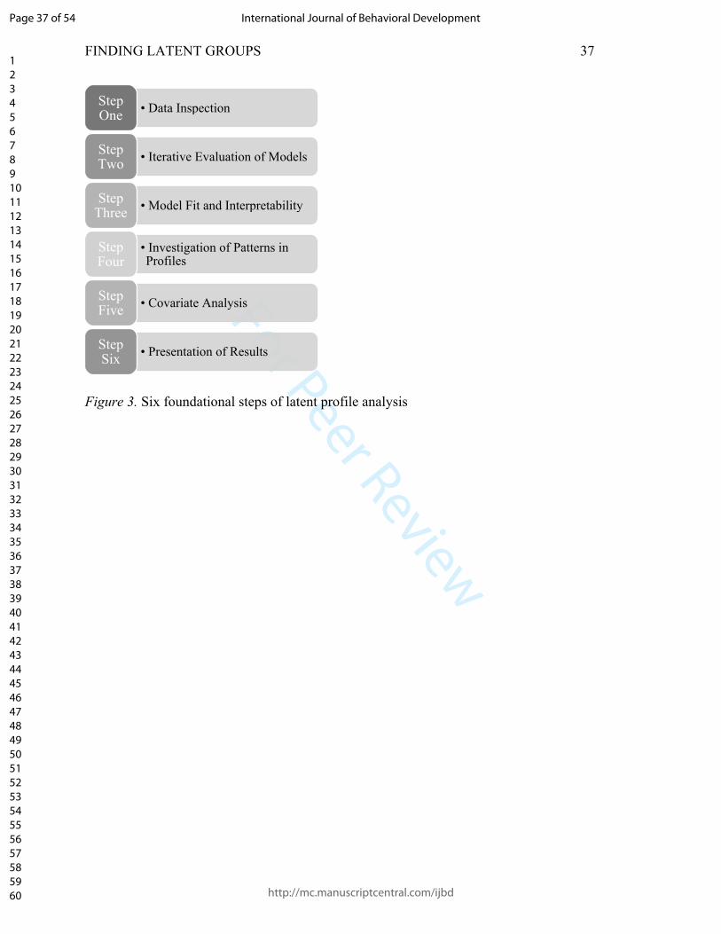
Steps of LPA

There are six general steps in the LPA process we will detail in this example (see Figure

3). Step one, as with all analyses, the data should be cleaned for analysis and checked for

standard statistical assumptions (e.g., normality of continuous variables, independence of

observations, etc.; see Osborne, 2012). In this example, item-level missing values were estimated

prior to the analysis process using maximum likelihood estimation in Mplus. Cases where all

items were missing for one composite variable (i.e., missingness at the composite level) were

estimated in the LPA process in Mplus utilizing full-information maximum likelihood (FIML).

Participants were removed from the analysis if values on all variables in the study were missing

(n = 4). As in other latent variable analyses, missing data can be handled by FIML or multiple

imputation, depending on what is best for the scenario. Multiple imputation is recommended

when a large dataset is being utilized to answer different research questions, planned missing

data designs were implemented, or the computational burden for model convergence will be

lessened utilizing imputed datasets rather than maximum likelihood estimation to handle the

missingness while estimating the model (Baraldi & Enders, 2010). In this example, we will

highlight how to utilize FIML with Mplus, which can often address individuals’ needs with

Page 15 of 54



123456789101112131415161718192021222324252627282930313233343536373839404142434445464748495051525354555657585960

For Peer Review


smaller datasets and the use of informative auxiliary variables (Baraldi & Enders, 2010; Howard,

Rhemtulla, & Little, 2015). Readers are referred to Osborne (2012) and Chapter 11 of the Mplus

user’s manual (Muthén & Muthén, 1998-2017) for further introduction to missing data issues.

Also of note in the present study is the use of composite variables as opposed to item-level data

as indicators in the model for simplicity (i.e., reduce complexity and increase model

convergence).

Step two involves evaluating a series of hypothetically plausible iterative LPA models,

starting with a model with one profile and typically ending with a model estimating five or six

profiles (Masyn, 2013; Tein, et al., 2013). Mplus syntax examples are provided in the Mplus

Version 8 user’s manual examples 7.9 and 7.12 (Muthén & Muthén, 1998-2017). Samples of the

basic LPA syntax can be found in Appendix A, and the syntax from this article’s example may

be found in Appendix B. In Mplus syntax, LPA is defined in two ways. First, the CLASSES

command is added after the USEVARIABLES command to specify the number of classes or

profiles being estimated in the model. So for the first one-profile model, CLASSES is set to c (1)

as shown in the example. For a two-profile model this would be CLASSES = c (2), and so on.

Second, the analysis TYPE is entered as MIXTURE, as LPA is a special type of mixture model.

Additionally, Mplus output options can be requested to support the LPA analysis process

(Muthén & Muthén, 1998-2017). TECH 1 is used for multiple analyses in Mplus as it provides

parameter specification and starting values for all estimated parameters in the model. This output

can be helpful in identifying estimation errors. TECH 8 provides the optimization history for

RANDOM, MIXTURE, and TWOLEVEL analyses in Mplus. TECH 11 is used to call for the

LMR test to compare the current model against the prior model estimated with k-1 classes or

profiles. Finally, TECH 14 calls for the bootstrap likelihood ratio test. Note that TECH 11 and

Page 16 of 54



123456789101112131415161718192021222324252627282930313233343536373839404142434445464748495051525354555657585960

For Peer Review


TECH 14 cannot be provided if there is only one class or profile in the model, so this option

must be removed from the syntax for the first model where only one profile is estimated (it is

provided in the one-profile example here for reference only). Additionally, in the SAVE line,

CPROBABILITIES is added to call for the class or profile probability estimates. This option

provides the posterior probabilities for each individual in each latent class or profile as well as

the most likely class membership for each individual in the sample. Also, note it is necessary to

change the SAVEDATA file name for each model run to avoid overwriting existing

SAVEDATA output files.

There are two other commands that are often used when conducting LPA that can assist

in obtaining a solution in Mplus. The first is using the STARTS subcommand under ANALYSIS

to adjust upward the number of either the initial stage starts in the maximization step and the

final stage optimizations in the likelihood step of the ML estimation (Muthén & Muthén, 1998-

2017). This helps the iteration process of the ML or MLR estimators reach convergence by

extending the number of attempts (Muthén & Muthén, 1998-2017). It is recommended that the

second value for the final stage optimizations be no more than a quarter of the initial stage starts

value (Muthén, 2010; Muthén & Muthén, 1998-2017).

Another approach that can assist in obtaining a solution for a model is providing start

values. There are two ways to specify start values. One is to manually specify start values, which

is done in the syntax by adding an asterisk (*) after a parameter in the model followed by the

start value. For example, Y ON X*.50 instructs Mplus to use .50 as the start value for the

regression coefficient Y ON X (i.e., X predicting Y). Another option, particularly if you have

attempted to model a solution that did not converge, is to use the values the model estimation did

reach for the parameter estimates as start values. Mplus always provides these start values in

Page 17 of 54



123456789101112131415161718192021222324252627282930313233343536373839404142434445464748495051525354555657585960

For Peer Review


TECH 1 output, SVALUES, and, when the model does not converge, under the MODEL

RESULTS (Muthén & Muthén, 1998-2017). TECH1 output start values is a good section to

examine if a particular parameter seems to be nearing an out of bounds estimation that results in

non-convergence (e.g., correlation too close to 1). The SVALUES section will provide the model

syntax including starting values based upon the model-estimated parameter values. This syntax

can be copied and pasted into the input syntax file under the MODEL command to inform

estimation in Mplus. As with TECH1, SVALUES can be included in the OUTPUT command

line of any model. When a model does not converge, the MODEL RESULTS output is formatted

for Mplus syntax so that it can be copied and pasted under the MODEL command in the syntax

file. To test if the model resulted from a local maxima in the estimation process, different,

random start values can be used to run the model again (see Hipp & Bauer, 2006 for further

information). Providing start values essentially helps the ML estimation process by informing the

Mplus estimator to pick-up where it left off, and hopefully reach model convergence.

In the example, a latent profile analysis was used for Research Question 1 to identify the

presence of latent profiles on measures of science interest, motivation, attitude, and academic

experiences. Model 1 was estimated with only one profile, Model 2 with two profiles, and so on

to Model 5 with five profiles. Model fit statistics are provided in Table 1.

INSERT TABLE 1 ABOUT HERE

Step three involves evaluating models to identify model fit and interpretability. In the

example presented, Model 4 was retained as the best model to fit the data based on the low

loglikelihood value, AIC, BIC, and SABIC values, high entropy value, non-significant LMR test,

the smallest class contained more than 5% of the sample, and the profiles were supported by

theory. The loglikelihood value revealed relatively large decreases until the difference between

Page 18 of 54



123456789101112131415161718192021222324252627282930313233343536373839404142434445464748495051525354555657585960

For Peer Review


Model 4 and 5. This is also true of the AIC and SABIC trend across models. BIC was marginally

lower for Model 4 in comparison to Model 5. All four of these statistics support models 4 and 5

as the better models. Entropy for both models 4 and 5 is above .80 and nearly the same. The

LMR and BLRT tests are significant for Model 4, which means the four-profile model is a better

representation than the three-profile model. However, LMR is not significant for Model 5, which

supports the more parsimonious Model 4 as a better fit than the less parsimonious Model 5. The

smallest profile in Model 4 comprises 16% (n = 44) of sample participants, whereas the smallest

profile for Model 5 comprises 2% (n = 6) of sample participants. When a small number of

participants from the sample are represented in a profile, as in Model 5, it is difficult to be

confident the profile represents a distinct grouping that might be generalizable to other samples.

Finally, profiles from Model 5 did not align with theory as well as Model 4 profiles, which

makes it difficult to justify and interpret (see Author, 2018).

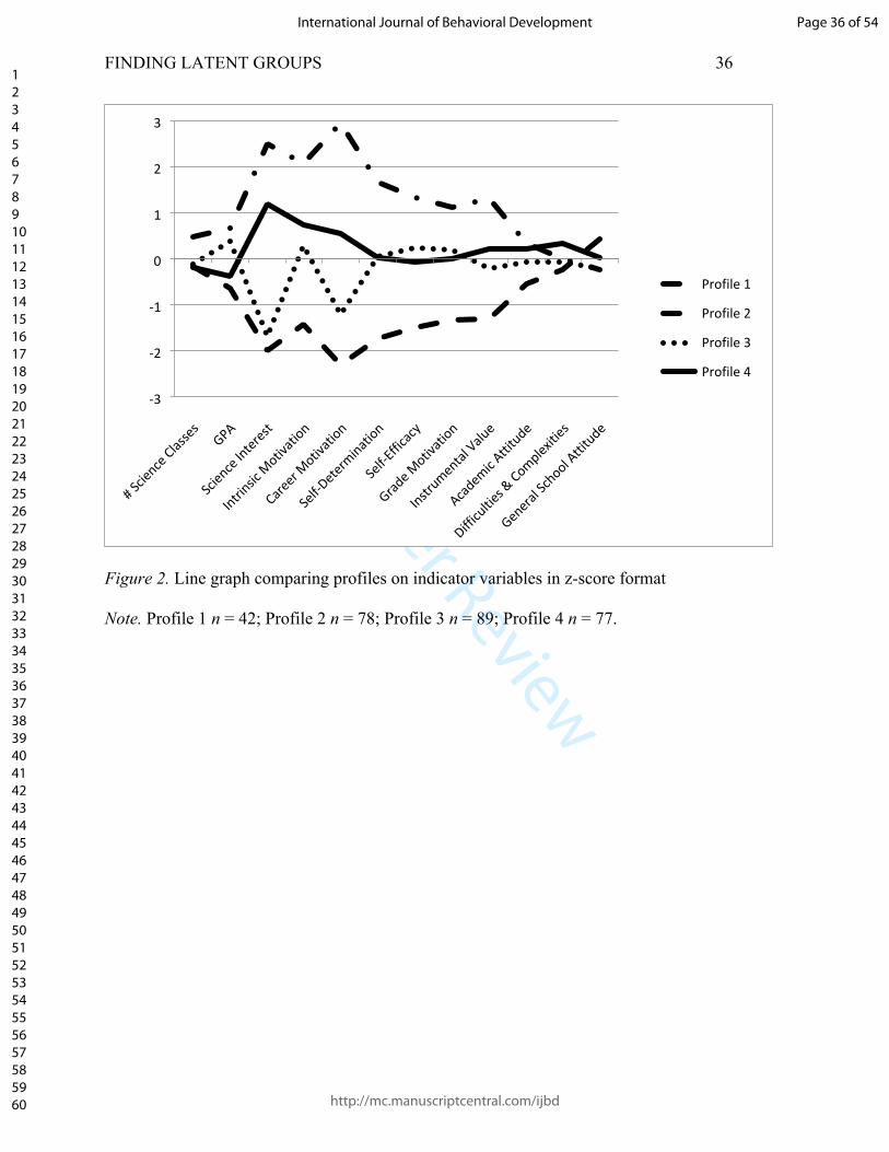
In step four of the LPA, the retained model is interpreted by examining patterns of the

profiles and weights of included variables in each profile. The four-profile model for this

example is detailed in Table 2. The means and standard deviations of variables used to create the

profiles are presented for each profile, and all were found to be statistically significant in the

model. Note that standard deviations are the same as they are constrained in Mplus by default.

The differences between the four latent groups are largely due to differences in interest,

motivation, and attitude towards science, which aligns with the theoretical approach used in the

study (see Figure 2).

It may be helpful in reporting LPA to provide names or labels for the profiles based on

the observed differences in included variables. However, researchers should be cautious in

providing names to avoid a naming fallacy, suggesting the label assigned to a profile is correct

Page 19 of 54



123456789101112131415161718192021222324252627282930313233343536373839404142434445464748495051525354555657585960

For Peer Review


and clearly understood, or a reification error suggesting the label represents a real construct

(Kline, 2011; Masyn, 2013). In the example, Profile 1 contains, on average, students with the

lowest level of interest in science, a more negative attitude and low motivation towards science,

and a low GPA, so was referred to as “Low Science Interest and GPA.” Profile 2 contains those

students with the highest interest in science, high attitude and motivation scores, and the highest

average GPA, so was called “High Science Interest and GPA”. Profile 3 students are low in

terms of science interest, but more towards the middle in science attitude and motivation, with a

GPA almost as high on average as seen in Profile 2. This profile was called “Low Science

Interest, High GPA.” Finally, Profile 4 contains students who are somewhat interested in science,

have mid-level attitudes and motivations towards science, and a GPA lower than Profile 3 but

higher than Profile 1. This profile was referred to as “Medium Science Interest and GPA.” These

profile names are illustrations of selecting names that are clear in the description without

overstating the profile or being cumbersome. It is important that when directional words are used

in naming (e.g., low, high, negative, positive) that they are accurate of not only the relative

relationship between the profiles in the sample but also of the absolute magnitude of the

variables/profiles that they are describing. Carefulness with naming ensures accuracy and clarity

when interpreting results and when generalizing results beyond the study sample.



Next, in step five, conduct a covariate analysis. This step should be included when: a) the

LPA analysis indicates there are profiles worth interpreting further, and b) there is a theoretical

reason to evaluate the impact of the covariates on the profiles. To add the covariates into the

model for concurrent analysis in Mplus, start with the syntax from step two. However, this time

add the variable information for covariates to the NAMES and USEVARIABLES lines.

Page 20 of 54



123456789101112131415161718192021222324252627282930313233343536373839404142434445464748495051525354555657585960

For Peer Review


Additionally, in the MODEL section of the syntax, specify the model relationships. For the

particular example included here, the two-step approach to covariate inclusion was used in the

original study (see Supplemental Files for Mplus syntax examples of all approaches). The syntax

subcommand “%OVERALL%” informs Mplus that the following lines describe the overall

model, as opposed to %class label%, which can be used to indicate an adjustment to class-

specific portions of the model such as constraining profiles to be equal on indicators or

estimating the variances of indicators across profiles (Muthén & Muthén, 1998-2017).

Covariates are entered into the model as predictors of c in the line “c ON X1 X2 X3”.

For the second research question in the example, profiles identified in Research Question

1 are further analyzed to evaluate effects of theoretically identified covariates. Covariates of

interest are: personality; cognitive ability, both verbal and spatial; sex; and socio-economic

status, as defined by parent education level and occupation. Covariates are added by regressing

the latent profile construct on the covariates (e.g., c ON X1 X2 X3). As the research is focused

on adolescents who would like to pursue science occupations, Profile 2 (Highest Science Interest

& GPA) was used as the reference group. Comparisons of all profiles against a specific profile as

a reference group are provided in the Mplus syntax by default, and the decision on which profile

is used as reference can be arbitrary in an exploratory analysis, or strategic to address a specific

research question as shown here. For this example, group difference values and statistical

significance tests presented in the output are tests between each profile and Profile 2 based upon

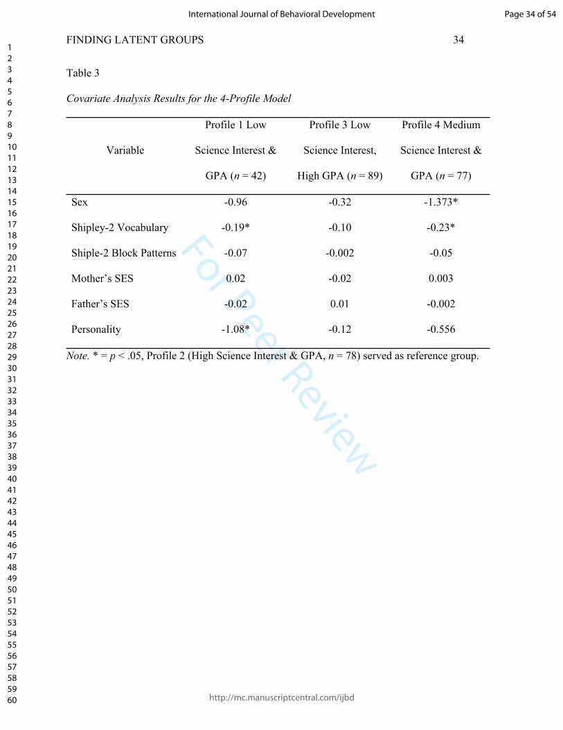
the research question of the study. The results of this covariate analysis are presented in Table 3.

However, individuals could replicate this approach using more than one profile as the reference

profile depending on their research question.


Page 21 of 54



123456789101112131415161718192021222324252627282930313233343536373839404142434445464748495051525354555657585960

For Peer Review


Based on this analysis, some covariates produce significant differences across profiles.

Results suggest sex is statistically significantly different between Profile 2 (Highest Science

Interest & GPA) and Profile 4 (Medium Science Interest & GPA), with more females

represented in the high science interest profile. This difference represents a difference in

membership by sex, not necessarily in measurement. If measurement across genders was of

research interest or concern, then a two-group (i.e., male and female) model could have been run

to test for measurement invariance (i.e., differences in parameter values by sex) of the latent

profile construct. Vocabulary scores are also statistically significantly different between Profile 2

(Highest Science Interest & GPA) and both Profile 1 (Lowest Science Interest & GPA) and

Profile 4 (Medium Science Interest & GPA). Negative coefficients indicate the high science

interest group tends to have higher vocabulary scores than the other two profiles. Finally,

personality is shown to be statistically, significantly different for Profile 1 (Lowest Science

Interest & GPA) as compared to Profile 2 (Highest Science Interest & GPA). A cross-tabulation

demonstrates the difference is that significantly more of the students considered “Well-Adjusted”

fall into the high science interest profile (see Author, 2018).

Step six is preparing the results for dissemination, the final step in the analysis.

Presentation of an LPA should generally follow the same sequence as the analysis. First, detail

data cleaning conducted, what assumptions are checked and the result, and how missing data are

handled. Include information about the software used for analysis (e.g., Mplus 8) and estimation

decisions made (e.g. changes to random starts, estimation method). Second, report steps taken to

estimate LPA models. How many models were included in the analysis, and why? Did any of the

models not converge? Finally, detail all decisions and problems that occurred in this step and

how any problems were addressed.

Page 22 of 54



123456789101112131415161718192021222324252627282930313233343536373839404142434445464748495051525354555657585960

For Peer Review


Third, report in a table all models that were estimated and the diversity of appropriate fit

indices that informed the gestalt decision process. We recommend including the loglikelihood

value, AIC, BIC, SABIC, LMR test, and BLRT. Preference in model retention should be given

to SABIC, BIC, and BLRT, based on the simulation studies discussed previously, but model

retention decisions can be strengthened with agreement between multiple pieces of information

(Kim, 2014; Masyn, 2013; Morgan, 2014; Nylund, Asparouhov, & Muthén, 2007). Entropy may

also be reported, particularly to support the accuracy of assigning individuals to profiles for

further analysis. Reporting the percentage of the sample that is found in the smallest profile can

also be a useful metric to support model retention decisions. There are other fit indices and

metrics that have been recommended, and these may be included as the researcher feels is

appropriate and/or as is common in a particular field’s literature (Marsh, et al., 2009; Masyn,

2013; Nylund, et al., 2007; Tein, et al., 2013; Vermunt & Magidson, 2002). Overall, a holistic

approach to reporting metrics should be used to support model retention decisions. Model

retention decisions should be justified by the majority of the metrics and indices included, even if

some do not suggest the same model (Kline, 2011; Marsh, et al., 2004; Masyn, 2013; Nylund, et

al., 2007; Schreiber, Nora, Stage, Barlow, & King, 2006).

Fourth, describe the profiles from the retained model. Pay attention to indicator variables

that appear to best differentiate between profiles and highlight the significant differences for the

reader. Tables and graphs can both be used to help the reader understand the relationships

between the profiles and the indicators. Naming the profiles is not necessary, but can be a helpful

way for readers to differentiate between groups and understand what indicators appear

meaningful. As the investigator, guide the reader in interpreting the profiles and implications for

differences observed.

Page 23 of 54



123456789101112131415161718192021222324252627282930313233343536373839404142434445464748495051525354555657585960

For Peer Review


Fifth, if applicable, detail the covariate analysis used. If covariates were added to the

LPA model and examined concurrently or in a three-step approach, report results of this analysis.

If individuals were assigned to profiles for further analysis independent of the LPA, justify this

process and clearly detail steps taken. How were individuals assigned to a profile? Were

individuals not clearly assigned to one profile, and if so how was this handled?


Conclusion

This article is intended to serve as a primer on the use of latent profile analysis (LPA) in

Mplus. LPA can be a very useful approach in research focused on personal behaviors and

characteristics as it uses person-level indicators to sort individuals into latent profiles based on

shared response patterns. LPA can be used in any social science research context where

individual differences and/or underlying patterns of shared behavior may be of interest. The

example presented here is one such application, but many other possibilities exist for

applications of LPA. LPA models of family functioning (Rybak, et al., 2017), employees’

commitment mindsets (Morin, Meyer, Creusier, & Bietry, 2016), adolescents’ coping strategies

Aldridge & Roesch, 2008), and school climate (Eck, Johnson, Bettencourt, & Johnson, 2017) are

examples of other psychological and behavioral phenomena that have been examined.

However, researchers should also be thoughtful of the assumptions and limitations of

LPA before using this method in their own work. LPA assumes the underlying latent profiles are

continuous, as opposed to categorical as would be found in latent class analysis. Additionally,

variables selected for inputs and covariates should be both theoretically supported as well as

appropriate for LPA. Using advanced statistical methods for their own sake does not improve

research practice, but using a technique like LPA when appropriate and theoretically justified can

Page 24 of 54



123456789101112131415161718192021222324252627282930313233343536373839404142434445464748495051525354555657585960

For Peer Review


increase our understanding of phenomena and uncover previously unknown differences or latent

groupings in data that may be meaningful to the field. This is not intended as an exhaustive

discussion of all current issues in LPA literature, and researchers should continue to evaluate

new approaches and improvements in LPA practice when undertaking a new analysis. However,

this resource is intended to be a starting place with a clear guide and discussion on the use of

LPA in applied research for novice researchers and reviewers new to this approach.

Page 25 of 54



123456789101112131415161718192021222324252627282930313233343536373839404142434445464748495051525354555657585960

For Peer Review


References

Aldridge, A. A. & Roesch, S. C. (2008). Developing coping typologies of minority adolescents:

A latent profile analysis. Journal of Adolescence, 31, 499-517. doi:

10.1016/j.adolescence.2007.08.005

Asparouhov, T., & Muthén, B. (2014). Auxiliary variables in mixture modeling: Three-step

approaches using M plus. Structural Equation Modeling: A Multidisciplinary

Journal, 21(3), 329-341.

Author (2018)

Baraldi, A. N. & Enders, C. K. (2010). An introduction to modern missing data analyses. Journal

of School Psychology, 48, 5 – 37. doi :10.1016/j.jsp.2009.10.001

Bauer, D. J., & Curran, P. J. (2004). The integration of continuous and discrete latent variable

models: Potential problems and promising opportunities. Psychological Methods, 9, 3-29.

doi: 10.1037/1082-989X.9.1.3

Bergman, L. R., & Magnusson, D. (1997). A person-oriented approach in research on

developmental psychopathology. Development and Psychopathology, 9, 291-319. doi:

10.1017/S095457949700206X

Bergman, L. R., Magnusson, D., & El Khouri, B. M. (2003). Studying individual development in

an interindividual context: A person-oriented approach. Mahwah, NJ: Psychology Press.

Celeux, G., & Soromenho, G. (1996). An entropy criterion for assessing the number of clusters

in a mixture model. Journal of Classification, 13, 195-212.

Clark, S. L., & Muthén, B. (2009). Relating latent class analysis results to variables not included

in the analysis. Available online: http://hbanaszak.mjr.uw.edu.pl/TempTxt/relatinglca.pdf

Collins, L. M., & Lanza, S. T. (2013). Latent class and latent transition analysis: With

Page 26 of 54



123456789101112131415161718192021222324252627282930313233343536373839404142434445464748495051525354555657585960

For Peer Review


applications in the social, behavioral, and health sciences. Hoboken, NJ: John Wiley &

Sons.

Christie, C. A., & Masyn, K. E. (2008). Latent profiles of evaluators’ self-reported practices. The

Canadian Journal of Program Evaluation, 23(2), 225-254.

Eck, K. V., Johnson, S. R., Bettencourt, A., & Johnson, S. L. (2017). How school climate relates

to chronic absence: A multi-level latent profile analysis. Journal of School Psychology, 61,

89-102. doi: 10.1016/j.jsp.2016.10.001

Gibson, W. A. (1959). Three multivariate models: Factor analysis, latent structure analysis, and

latent profile analysis. Psychometrika, 24, 229-252.

Gudicha, D. (2015). Power analysis methods for tests in latent class and latent Markov models

Ridderkerk, The Netherlands: Ridderprint BV.

Henson, R. K., Hull, D. M., & Williams, C. S. (2010). Methodology in our education research

culture: Toward a stronger collective quantitative proficiency. Educational

Researcher, 39(3), 229-240.

Howard, W. J., Rhemtulla, M., & Little, T. D. (2015). Using principal components as auxiliary

variables in missing data estimation. Multivariate Behavioral Research, 50(3), 285-299.

Kim, S. Y. (2014). Determining the number of latent classes in single-and multiphase growth

mixture models. Structural Equation Modeling, 21(2), 263-279. doi:

10.1080/10705511.2014.882690

Kline, R. B. (2011). Principles and practice of structural equation modeling (3rd Ed.). New

York, NY: Guilford Press.

Lo, Y., Mendell, N. R., & Rubin, D. B. (2001). Testing the number of components in a normal

mixture. Biometrika, 88, 767-778.

Page 27 of 54



123456789101112131415161718192021222324252627282930313233343536373839404142434445464748495051525354555657585960

For Peer Review


MacCallum, R. C., Browne, M. W., & Sugawara, H. M. (1996). Power analysis and

determination of sample size for covariance structure modeling. Psychological

methods, 1(2), 130-149.

Marsh, H. W., Hau, K. T., & Wen, Z. (2004). In search of golden rules: Comment on hypothesis-

testing approaches to setting cutoff values for fit indexes and dangers in overgeneralizing

Hu and Bentler's (1999) findings. Structural equation modeling, 11, 320-341. doi:

10.1207/s15328007sem1103_2

Marsh, H. W., Lüdtke, O., Trautwein, U., & Morin, A. J. (2009). Classical latent profile analysis

of academic self-concept dimensions: Synergy of person-and variable-centered approaches

to theoretical models of self-concept. Structural Equation Modeling, 16, 191-225. doi:

10.1080/10705510902751010

Masyn, K. E. (2013). Latent class analysis and finite mixture modeling. In T. Little (Eds), The

Oxford Handbook of Quantitative Methods (551-611). New York, NY: Oxford University

Press.

Masyn, K. E. (2017). Measurement invariance and differential item functioning in latent class

analysis with stepwise multiple indicator multiple cause modeling. Structural Equation

Modeling: A Multidisciplinary Journal, 24(2), 180-197.

McLachlan, G. J. (1987). On bootstrapping the likelihood ratio test statistic for the number of

components in a normal mixture. Applied Statistics, 36, 318-324. doi: 10.2307/2347790

McLarnon, M. J. W. & O’Neill, T. A. (2018). Extensions of auxiliary variable approaches for the

investigation of mediation, moderation, and conditional effects in mixture models.

Organizational Research Methods, 21(4), 955-982. doi: 10.1177/1094428118770731.

Morgan, G. B. (2015). Mixed mode latent class analysis: An examination of fit index

Page 28 of 54



123456789101112131415161718192021222324252627282930313233343536373839404142434445464748495051525354555657585960

For Peer Review


performance for classification. Structural Equation Modeling, 22(1), 76-86. doi:

10.1080/10705511.2014.935751

Morin, A. J. S., Meyer, J. P., Creusier, J., & Bietry, F. (2016). Multiple-group analysis of

similarity in latent profile solutions. Organizational Research Methods, 19(2), 231-254.

doi: 10.1177/1094428115621148

Muthén, L. (2010, November 29). Re: Latent profile analysis [Online discussion group].

Retrieved from

http://www.statmodel.com/discussion/messages/13/115.html?1507757139

Muthén, L.K. and Muthén, B.O. (1998-2017). Mplus user’s guide. (8th Ed.). Los Angeles, CA:

Muthén & Muthén

Nylund, K. L., Asparouhov, T., & Muthén, B. O. (2007). Deciding on the number of classes in

latent class analysis and growth mixture modeling: A Monte Carlo simulation

study. Structural Equation Modeling, 14(4), 535-569. doi: 10.1080/10705510701575396

Nylund-Gibson, K. & Choi, A. Y. (2018). Ten frequently asked questions about latent class

analysis. Translational Issues in Psychological Sciences, 4(4), 440-461. doi:

10.1037/tps0000176

Nylund-Gibson, K. & Masyn, K. E. (2016). Covariates and mixture modeling: Results of a

simulation study exploring the impact of misspecified effects on class enumeration.

Structural Equation Modeling, 23, 782-797. doi: 10.1080/10705511.2016.1221313

Nylund-Gibson, K., Grimm, R., Quirk, M., & Furlong, M. (2014). A latent transition mixture

model using the three-step specification. Structural Equation Modeling: A Multidisciplinary

Journal, 21, 1-16. doi: 10.1080/10705511.2014.915375

Oberski, D. (2016). Mixture models: Latent profile and latent class analysis. In J. Robertson and

Page 29 of 54



123456789101112131415161718192021222324252627282930313233343536373839404142434445464748495051525354555657585960

For Peer Review


M. Kaptein (Eds.), Modern Statistical Methods for HCI. Springer International Publishing:

Cham, Switzerland.

Osborne, J. W. (2012). Best practices in data cleaning: A complete guide to everything you need

to do before and after collecting your data. Thousand Oaks, CA: Sage.

Osterlind, S. J., & Everson, H. T. (2009). Differential item functioning (Vol. 161). Sage

Publications.

Park, J., & Yu, H. T. (2017). Recommendations on the sample sizes for multilevel latent class

models. Educational and Psychological Measurement, Available online:

http://journals.sagepub.com/doi/abs/10.1177/0013164417719111. doi:

10.1177/0013164417719111.

Peugh, J., & Fan, X. (2015). Enumeration index performance in generalized growth mixture

models: A Monte Carlo test of Muthén’s (2003) hypothesis. Structural Equation

Modeling, 22(1), 115-131. doi: 10.1080/10705511.2014.919823

Preacher, K. J., & Coffman, D. L. (2006, May). Computing power and minimum sample size for

RMSEA [Computer software]. Available from http://quantpsy.org/.

Rybak, T. M., Ali, J. S., Berlin, K. S., Klages, K. L., Banks, G. G., Kamody, R. C., Ferry, R. J.,

Alemzadeh, R., & Diaz-Thomas, A. M. (2017). Patterns of family functioning and

diabetes-specific conflict in relation to glycemic control and health-related quality of life

among youth with Type I Diabetes. Journal of Pediatric Psychology, 42(1), 40-51. doi:

10.1093/jpepsy/jsw071

Schreiber, J. B., Nora, A., Stage, F. K., Barlow, E. A., & King, J. (2006). Reporting structural

equation modeling and confirmatory factor analysis results: A review. Journal of

Educational Research, 99, 323-338.

Page 30 of 54



123456789101112131415161718192021222324252627282930313233343536373839404142434445464748495051525354555657585960

For Peer Review


Sterba, S. K. (2013). Understanding linkages among mixture models. Multivariate Behavioral

Research, 48, 775-815. doi:10.1080/00273171.2013.827564

Tein, J. Y., Coxe, S., & Cham, H. (2013). Statistical power to detect the correct number of

classes in latent profile analysis. Structural Equation Modeling, 20, 640-657. doi:

10.1080/10705511.2013.824781

Vermunt, J. K. (2010). Latent class modeling with covariates: Two improved three-step

approaches. Political Analysis, 18(4), 450-469.

Vermunt, J. K., & Magidson, J. (2002). Latent class cluster analysis. In J. Hagenaars, & A.

McCutcheon (Eds.), Applied latent class analysis. (pp. 89-106). Cambridge: Cambridge

University Press.

Vincent, W. J. & Weir, J. P. (2012). Statistics in Kinesiology (4th Ed). Champaign, IL: Human

Kinetics.

Page 31 of 54



123456789101112131415161718192021222324252627282930313233343536373839404142434445464748495051525354555657585960

For Peer Review


Table 1

LPA Model Fit Summary for Research Question 1

Model Log likelihood

AIC BIC SABIC Entropy Smallest Class %

LMR p-value

LMR Meaning

BLRT p-value

BLRT Meaning

1 -8909.94 17867.88 17955.96 17879.85 - - - -

2 -8507.38 17088.75 17224.54 17107.21 0.89 45% <0.001 2 > 1 <0.001 2 > 1

3 -8370.30 16840.60 17024.10 16865.54 0.90 30% 0.002 3 > 2 <0.001 3 > 2

4 -8290.15 16706.31 16937.51 16737.73 0.89 16% 0.010 4 > 3 <0.001 4 > 3

5 -8253.86 16659.72 16938.63 16697.62 0.90 2% 0.614 5 < 4 <0.001 5 > 4

Note. n = 295, The Lo-Mendell Ruben (LMR) test and the bootstrap likelihood ratio test (BLRT)

compare the current model to a model with k-1 profiles.

Page 32 of 54



123456789101112131415161718192021222324252627282930313233343536373839404142434445464748495051525354555657585960

For Peer Review


Table 2

Four-Profile Model Results

Variable

Profile 1

Low Science

Interest & GPA

(n = 42)

Profile 2

High Science

Interest & GPA

(n = 78)

Profile 3

Low Science

Interest, High

GPA

(n = 89)

Profile 4

Medium

Science

Interest & GPA

(n =77)

Number of Science Classes 3.74 (0.88) 4.31 (0.88) 3.78 (0.88) 3.71 (0.88)

GPA 2.95 (0.63) 3.77 (0.63) 3.59 (0.63) 3.11 (0.63)

Science Interest 3.65 (0.52) 1.32 (0.52) 3.49 (0.52) 2.00 (0.52)

Science Motivation

Intrinsic Motivation 10.31 (3.05) 21.03 (3.05) 15.58 (3.05) 16.91 (3.05)

Career Motivation 8.18 (2.84) 23.06 (2.84) 11.27 (2.84) 16.27 (2.84)

Self-Determination 9.19 (3.00) 19.37 (3.00) 14.50 (3.00) 14.43 (3.00)

Self-Efficacy 12.63 (3.22) 21.75 (3.22) 18.23 (3.22) 17.26 (3.22)

Grade Motivation 12.74 (3.70) 21.80 (3.70) 18.37 (3.70) 17.62 (3.70)

Attitude Towards Science

Instrumental Value 41.36 (6.75) 59.05 (6.75) 48.80 (6.75) 51.67 (6.75)

Academic 19.20 (5.39) 23.89 (5.39) 21.73 (5.39) 23.24 (5.39)

Difficulties & Complexities 20.15 (4.52) 21.25 (4.52) 20.88 (4.52) 22.75 (4.52)

General School 11.23 (2.71) 9.433 (2.71) 9.54 (2.71) 10.16 (2.71)

Note. Values respresenting highest positive response in bold (Science Interest and ATS-General School

are reverse coded). Means and standard deviations for variables across all profiles: Number of Science

Classes M=3.78 (SD=0.90), GPA M=3.41 (SD=0.70), Science Interest M=2.00 (SD=0.50), Intrinsic

Motivation M=16.58 (SD=4.60), Career Motivation M=15.32 (SD=6.11), Self-Determination M=14.95

(SD=4.42), Self-Efficacy M=18.02 (SD=4.35), Grade Motivation M=18.20 (SD=4.69), Instrumental

Value M=51.18 (SD=8.90), Academic M=22.34 (SD=5.63), Difficulties & Complexities M=21.38

(SD=4.62), General School M=9.94 (SD=2.78 )

Page 33 of 54



123456789101112131415161718192021222324252627282930313233343536373839404142434445464748495051525354555657585960

For Peer Review


Table 3

Covariate Analysis Results for the 4-Profile Model

Variable

Profile 1 Low

Science Interest &

GPA (n = 42)

Profile 3 Low

Science Interest,

High GPA (n = 89)

Profile 4 Medium

Science Interest &

GPA (n = 77)

Sex -0.96 -0.32 -1.373*

Shipley-2 Vocabulary -0.19* -0.10 -0.23*

Shiple-2 Block Patterns -0.07 -0.002 -0.05

Mother’s SES 0.02 -0.02 0.003

Father’s SES -0.02 0.01 -0.002

Personality -1.08* -0.12 -0.556

Note. * = p < .05, Profile 2 (High Science Interest & GPA, n = 78) served as reference group.

Page 34 of 54



123456789101112131415161718192021222324252627282930313233343536373839404142434445464748495051525354555657585960

For Peer Review


rr r r

Interest Motivation Attitude Academic

Experienc

ec

0 0 0 0

Interest in

Science

Items

Science

Motivation

Questionnair

e

Attitudes

Towards

Science

Science

Courses

Taken and

GPA

a1 a2 a3 a4

Sex

Personality

Profile

Cognitive

Ability

SES

g1

g2

g3

g4

Figure 1. Example of LPA model with covariates

Page 35 of 54



123456789101112131415161718192021222324252627282930313233343536373839404142434445464748495051525354555657585960

For Peer Review


# Science

Classes

GPA

Science

Interest

Intrinsic

Motiv

ation

Career M

otivati

on

Self-D

eterminati

on

Self-E

fficac

y

Grade M

otivati

on

Instrumental

Value

Academic A

ttitude

Difficu

lties &

Complexities

General Sc

hool Atti

tude

-3

-2

-1

0

1

2

3

Profile 1

Profile 2

Profile 3

Profile 4

Figure 2. Line graph comparing profiles on indicator variables in z-score format

Note. Profile 1 n = 42; Profile 2 n = 78; Profile 3 n = 89; Profile 4 n = 77.

Page 36 of 54



123456789101112131415161718192021222324252627282930313233343536373839404142434445464748495051525354555657585960

For Peer Review


• Data InspectionStep One

• Iterative Evaluation of ModelsStep Two

• Model Fit and InterpretabilityStep Three

• Investigation of Patterns in Profiles

Step Four

• Covariate Analysis Step Five

• Presentation of ResultsStep Six

Figure 3. Six foundational steps of latent profile analysis

Page 37 of 54



123456789101112131415161718192021222324252627282930313233343536373839404142434445464748495051525354555657585960

For Peer Review


Appendix A: Mplus Syntax Simple Example

One Profile LPA Model

TITLE: LPA generic 2 profile syntax example

DATA:FILE IS data.dat; ! Specifies file location for data file. Make sure data is in format appropriate for Mplus analysis ! per Mplus manual. This data file is in individual format (one row of data per participant)

VARIABLE:NAMES ARE Y1-Y5 X1-X3; ! All variables included in data file should be named here. !X1-X3 is shorthand for X1 through X3.USEVARIABLES ARE Y1-Y5; ! Only variables intended for use in the analysis should be listed hereCLASSES = c (2); ! This is where you instruct Mplus on how many classes/profiles are being estimated. Initial ! model contains only one class/profile, thus it would be CLASSES = c (1). Above specifies two !profiles, and for each further iterative models the number in parentheses increases by one, so !three profiles/classes would be c (3), and so on.

MISSING ARE .; ! Used to communicate how missing data is coded in data file. Here shown with a “.” which is ! all that is included in each cell with missing data in the data file

ANALYSIS:TYPE = MIXTURE; ! LPA is a version of mixture modeling, and this instructs Mplus to analyze in this way

ESTIMATOR = MLR;!FIML robust to non-normal data

STARTS = 1000 250;STITERATIONS = 500;! Default number of starts for each step of the ML estimation. First STARTS value specifies the !number of unique start values to start with, the 250 represents the 250 best unique start values !carrying forward to completion. The STITERATIONS specifies the number of ML iteration !steps for those 250 selected start values to go through to be able to converge. This is a! !maximum number of iteration; if a model converges in less than 500 iterations it will stop !before reaching 500 iterations. !These values can be increased … see “Four-Profile Final Model with Covariate Analysis !Syntax” for an example.

LRTSTARTS = 2 1 50 10;LRTBOOSTRAP = 250;

Page 38 of 54



123456789101112131415161718192021222324252627282930313233343536373839404142434445464748495051525354555657585960

For Peer Review


!The above start values are for the defaults for the LRT statistic being run to compare the current !model fit with the model fit of a model with one less class (k-1). The BOOTSTRAP statement !specifies the number of bootstrap draws to inform Mplus’ bootstrapped LRT results.

MODEL:!For a default Mplus model the LPA model does not need to be specified. However, it can be. !The model can also be modified from the Mplus default of estimating the indicator means (uniquely across profiles) and variances (constrained across profiles), as well as the latent !profile mean.

%OVERALL%

[Y1-Y5]; !estimates the 5 indicators means for each profile. Without a label after the brackets, !the means are freely estimated in each profile, not constrained.

Y1-Y5 (Var1-Var5); !Label Var1-Var5 constrains the estimates of the variances across the !profiles to be equal.

OUTPUT:TECH1 TECH8 TECH11 TECH14;! TECH1 provides parameter specifications and starting values for the analysis ! TECH8 provides optimization history for this analysis type!TECH11 provides LRT results!TECH14 provides bootstrapped LRT test

SAVEDATA:FILE IS LPA2.dat;! Tells Mplus where to save the output files from the analysis SAVE = CPROBABILITIES; ! The above command lines are to save the most likely profile membership for each participant ! and the posterior probabilities for their membership in each latent profile.

Page 39 of 54



123456789101112131415161718192021222324252627282930313233343536373839404142434445464748495051525354555657585960

For Peer Review


LPA Model with Covariate Analysis

TITLE: LPA generic syntax example with covariates

DATA:FILE IS data.dat; ! Specifies file location for data file. Make sure data is in format appropriate for Mplus analysis ! per Mplus manual. This data file is in individual format (one row of data per participant)

VARIABLE:NAMES ARE Y1-Y5 X1-X3; ! All variables included in data file should be named hereUSEVARIABLES ARE Y1-Y5 X1-X3; ! All variables intended for use in the analysis should be listed here. The covariate variables are !included for this particular version of syntax though they were not included during the class !enumeration steps.

CLASSES = c (4); ! This is where you instruct Mplus on how many classes/profiles are being estimated. !For this version of covariate inclusion you would retain the best fitting model from prior !analyses without covariates!In this example a model with 4 profiles/classes so CLASSES= c (4)

MISSING ARE .; ! Used to communicate how missing data is coded in data file, here shown with a “.” and this is ! included in in each cell with missing data in the data file

ANALYSIS:TYPE = MIXTURE; ! LPA is a version of mixture modeling, and this instructs Mplus to analyze in this way!See above model ANALYSIS syntax for additional options that can be added to improve model !estimation and convergence.

MODEL: %OVERALL% c ON X1 X2 X3; ! New inclusion here instructs Mplus to run the model as before and then add the covariates X1 ! X2 and X3 as predictors of “c” classes/profiles

OUTPUT:TECH1 TECH8 TECH11 TECH14;! TECH1 provides parameter specifications and starting values for the analysis ! TECH8 provides optimization history for this analysis type! TECH11 provides LMR test comparing this model to the previous model. ! (cannot be calculated with one profile model)

Page 40 of 54



123456789101112131415161718192021222324252627282930313233343536373839404142434445464748495051525354555657585960

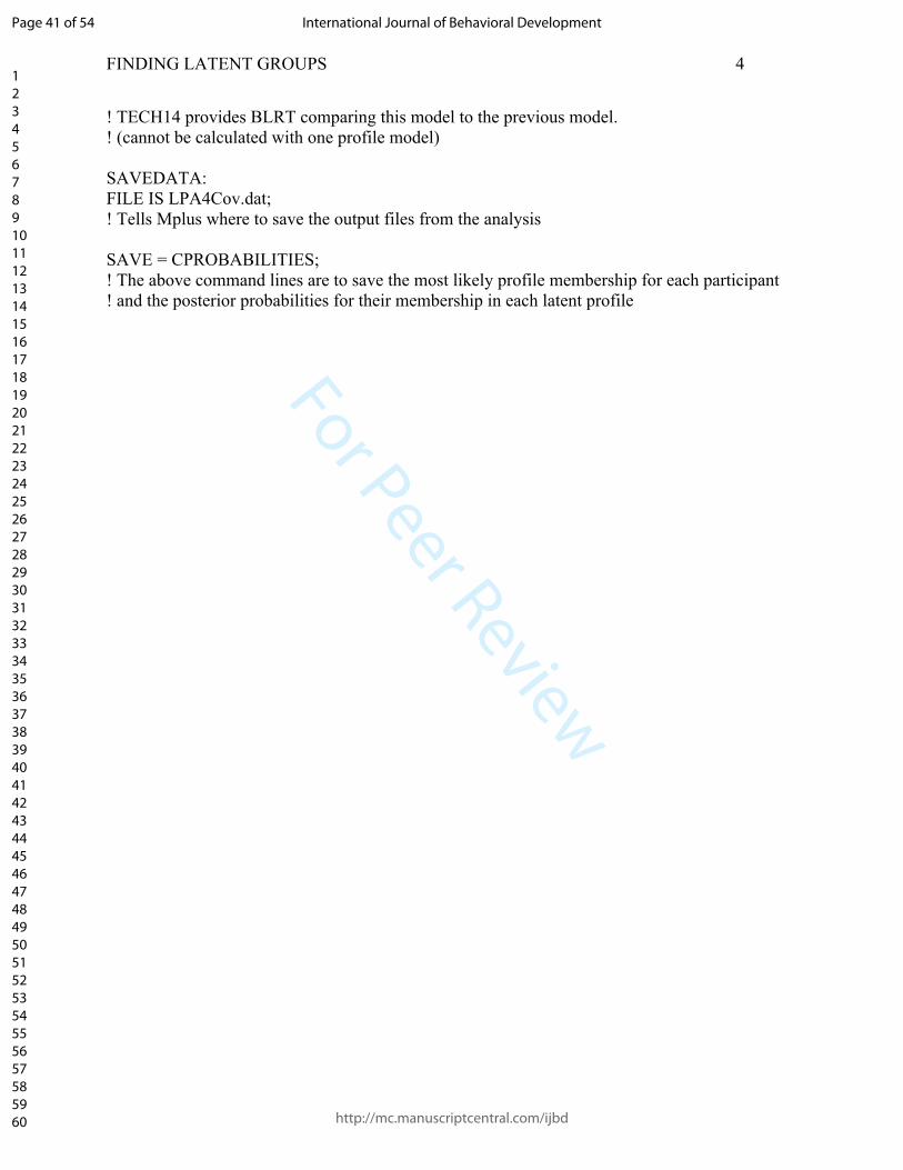
For Peer Review


! TECH14 provides BLRT comparing this model to the previous model. ! (cannot be calculated with one profile model)

SAVEDATA:FILE IS LPA4Cov.dat;! Tells Mplus where to save the output files from the analysis

SAVE = CPROBABILITIES; ! The above command lines are to save the most likely profile membership for each participant ! and the posterior probabilities for their membership in each latent profile

Page 41 of 54



123456789101112131415161718192021222324252627282930313233343536373839404142434445464748495051525354555657585960

For Peer Review


Appendix B: Mplus Syntax from Example Study

Enumeration Step

Two-Profile LPA Syntax 4 ClassesTITLE: Latent Profile Analysis Model 1, 2 Profile, Students

DATA: FILE IS Mplus_LPA_RQ1_Final.csv;! Specifies file location for data file. Make sure data is in format appropriate for Mplus analysis ! per Mplus manual. This data file is in individual format (one row of data per participant)

VARIABLE: NAMES ARE ID Sex MomEd MomOcc DadEdDadOcc ClassNum GPA Plans IPIP_N IPIP_E IPIP_O IPIP_AIPIP_C SM_IM SM_CM SM_SD SM_SE SM_GM ATS_IVATS_AP ATS_DC ATS_GS Ship_V Ship_B MomSESDadSES;! All variables included in data file should be named here.

USEVARIABLES ClassNum GPA Plans SM_IM SM_CM SM_SD SM_SE SM_GM ATS_IV ATS_AP ATS_DC ATS_GS; ! Selecting variables to use in the model (all profile indicators, no covariates at this stage)

CLASSES=c(4); ! This is where you instruct Mplus on how many classes/profiles are being estimated. Initial ! model contains only one class/profile, thus it would be CLASSES = c (1). Above specifies four !profiles, and for each further iterative models the number in parentheses increases by one.

MISSING ARE .; ! Used to communicate how missing data is coded in data file. Here shown with a “.” which is ! all that is included in each cell with missing data in the data file

ANALYSIS:TYPE=MIXTURE;! LPA is a version of mixture modeling, and this instructs Mplus to analyze in this way

ESTIMATOR = MLR;!FIML robust to non-normal data

STARTS = 1000 250;STITERATIONS = 500;! Default number of starts for each step of the ML estimation. First STARTS value specifies the !number of unique start values to start with, the 250 represents the 250 best unique start values !carrying forward to completion. The STITERATIONS specifies the number of ML iteration

Page 42 of 54



123456789101112131415161718192021222324252627282930313233343536373839404142434445464748495051525354555657585960

For Peer Review


!steps for those 250 selected start values to go through to be able to converge. This is a! !maximum number of iteration; if a model converges in less than 500 iterations it will stop !before reaching 500 iterations. !These values can be increased … see “Four-Profile Final Model with Covariate Analysis !Syntax” for an example.

LRTSTARTS = 2 1 50 10;LRTBOOSTRAP = 250;!The above start values are for the defaults for the LRT statistic being run to compare the current !model fit with the model fit of a model with one less class (k-1). The BOOTSTRAP statement !specifies the number of bootstrap draws to inform Mplus’ bootstrapped LRT results.

MODEL:!For a default Mplus model the LPA model does not need to be specified. However, it can be. !The model can also be modified from the Mplus default of estimating the indicator means !(uniquely across profiles) and variances (constrained across profiles), as well as the latent !profile mean. The syntax below specifies the Mplus defaults.

%OVERALL%

[ClassNum GPA Plans SM_IM SM_CM SM_SD SM_SE SM_GM ATS_IV ATS_AP ATS_DC ATS_GS]; !estimates the indicator means for each profile. Without a label !after the brackets, the means are freely estimated in each profile, not constrained.

ClassNum GPA Plans SM_IM SM_CM SM_SD SM_SE SM_GM ATS_IV ATS_AP ATS_DC ATS_GS (Var1-Var12); !Label Var1-Var12 constrains the estimates of the !variances across the profiles to be equal.

OUTPUT:TECH1 TECH8 TECH11 TECH14; ! TECH1 provides parameter specifications and starting values for the analysis ! TECH8 provides optimization history for this analysis type!TECH11 provides LRT results!TECH14 provides bootstrapped LRT test

SAVEDATA:FILE IS LPA1_2_FINAL.dat; ! Tells Mplus where to save the output files from the analysis

SAVE = CPROBABILITIES;! The above command lines are to save the most likely profile membership for each participant ! and the posterior probabilities for their membership in each latent profile.

Page 43 of 54



123456789101112131415161718192021222324252627282930313233343536373839404142434445464748495051525354555657585960

For Peer Review


Appendix C: Mplus Syntax from Example Study

Four-Profile Final Model with BCH Covariate Analysis Syntax

Step 2, after enumeration phase completed is to create a file with the BCH weights and covariates in the same file.

TITLE: Latent Profile Analysis Model 1, 4 Profile, Students

DATA: FILE IS Mplus_LPA_RQ1_Final.csv;

VARIABLE: NAMES ARE ID Sex MomEd MomOcc DadEdDadOcc ClassNum GPA Plans IPIP_N IPIP_E IPIP_O IPIP_AIPIP_C SM_IM SM_CM SM_SD SM_SE SM_GM ATS_IVATS_AP ATS_DC ATS_GS Ship_V Ship_B MomSESDadSES;

USEVARIABLES ClassNum GPA Plans SM_IM SM_CM SM_SD SM_SE SM_GM ATS_IV ATS_AP ATS_DC ATS_GS;

CLASSES=c(4); ! Four latent profiles specified, based on results of original iterative modeling process

AUXILLARY = Sex Ship_V Ship_B MomSES DadSES PersProf;! Now, covariates are included in the AUXILIARY statement so that they will be included in the !datafile outputted by the SAVEDATA command at the bottom of the syntax file.

MISSING ARE .;

ANALYSIS:TYPE=MIXTURE;STARTS=2000 500; ! Added increased number of starts for each step of the ML estimation in response to message ! about possible convergence issue noted in output

MODEL:!Want to run the model that was decided upon through the enumeration phase.

!For a default Mplus model the LPA model does not need to be specified. However, it can be. !The model can also be modified from the Mplus default of estimating the indicator means !(uniquely across profiles) and variances (constrained across profiles), as well as the latent !profile mean. The syntax below specifies the Mplus defaults.

%OVERALL%

Page 44 of 54



123456789101112131415161718192021222324252627282930313233343536373839404142434445464748495051525354555657585960

For Peer Review




OUTPUT:TECH1 TECH8 TECH11 TECH 14;

SAVEDATA:FILE IS LPA1_4_FINAL_Cov.dat;SAVE = bchweights;!This statement makes sure that the weights of the indicators for each of the profiles. The bch !weights are based upon the “Classification Probabilities for the Most Likely Latent Class !Membership (Column) by Latent Class (Row)”. These are used in the next modeling step to !specify the profiles so that they are not affected by the inclusion of the covariates in the model.

Page 45 of 54



123456789101112131415161718192021222324252627282930313233343536373839404142434445464748495051525354555657585960

For Peer Review


Mplus Syntax from Example Study

Four-Profile Final Model with BCH Covariate Analysis Syntax

!Step 3: Estimating covariate and profile relationships


DATA: FILE IS LPA1_4_FINAL_Cov.dat;!Note: the file name changed to the file outputted from the model run above in Step 2.

VARIABLE: NAMES ARE ID Sex MomEd MomOcc DadEdDadOcc ClassNum GPA Plans IPIP_N IPIP_E IPIP_O IPIP_AIPIP_C SM_IM SM_CM SM_SD SM_SE SM_GM ATS_IVATS_AP ATS_DC ATS_GS Ship_V Ship_B MomSESDadSES W1-W4 MLC;!The BCH weights (W1-W4) are included at the end of the datafile.

USEVARIABLES Sex Ship_V Ship_B MomSES DadSES PersProf W1-W4;

! Now, covariates are included in the USEVARIABLES statement. The BCH weights (W1-W4) !are also included. Because the BCH weights are included, the original indicators do not need to !be included in the usevariables. The BCH weights are unique to the individual, therefore !retaining the classification uncertainty present in the enumeration step in this model. CLASSES=c(4); ! Four latent profiles specified, based on results of original iterative modeling process

TRAINING = W1-W4 (bch);

MISSING ARE .;

ANALYSIS:TYPE=MIXTURE;STARTS=0;! Note. Starts now 0 because the BCH weights are specifying the classes based upon the prior !model run.

MODEL:

%OVERALL%C ON Sex Ship_V Ship_B MomSES DadSES PersProf;!Latent profiles regressed on the covariate variables. These are uniquely estimated for each class.

Page 46 of 54



123456789101112131415161718192021222324252627282930313233343536373839404142434445464748495051525354555657585960

For Peer Review


!If there are additional relationships (e.g., PersProf ON Sex) that should be estimated uniquely in !one or more of the classes (i.e., not constrained across classes), then the class-specific syntax !can be added below.


Page 47 of 54



123456789101112131415161718192021222324252627282930313233343536373839404142434445464748495051525354555657585960

For Peer Review


Appendix D: Mplus Syntax from Example Study

Four-Profile Final Model with VAM (three-step) Covariate Analysis Syntax

Step 2, after enumeration phase completed is to create a file with the class posterior probabilities along with the covariates by including them as auxiliary variables.


DATA: FILE IS Mplus_LPA_RQ1_Final.csv;

VARIABLE: NAMES ARE ID Sex MomEd MomOcc DadEdDadOcc ClassNum GPA Plans IPIP_N IPIP_E IPIP_O IPIP_AIPIP_C SM_IM SM_CM SM_SD SM_SE SM_GM ATS_IVATS_AP ATS_DC ATS_GS Ship_V Ship_B MomSESDadSES;

USEVARIABLES ClassNum GPA Plans SM_IM SM_CM SM_SD SM_SE SM_GM ATS_IV ATS_AP ATS_DC ATS_GS;


AUXILLARY = Sex Ship_V Ship_B MomSES DadSES PersProf;! Now, covariates are included in the AUXILIARY statement so that they will be included in the !datafile outputted by the SAVEDATA command at the bottom of the syntax file.

MISSING ARE .;

ANALYSIS:TYPE=MIXTURE;STARTS=2000 500; ! Added increased number of starts for each step of the ML estimation in response to message ! about possible convergence issue noted in output

MODEL:!Want to run the model that was decided upon through the enumeration phase.

!For a default Mplus model the LPA model does not need to be specified. However, it can be. !The model can also be modified from the Mplus default of estimating the indicator means !(uniquely across profiles) and variances (constrained across profiles), as well as the latent !profile mean. The syntax below specifies the Mplus defaults.

%OVERALL%

Page 48 of 54



123456789101112131415161718192021222324252627282930313233343536373839404142434445464748495051525354555657585960

For Peer Review





SAVEDATA:FILE IS LPA1_4_FINAL_Cov_VAM.dat;SAVE = CPROB;!This statement makes sure that the class posterior probabilities and most likely classification (MODAL column) are saved along with the variables in the USE and AUXILIARY statements.

Page 49 of 54



123456789101112131415161718192021222324252627282930313233343536373839404142434445464748495051525354555657585960

For Peer Review


Mplus Syntax from Example Study

Four-Profile Final Model with VAM (three-step) Covariate Analysis Syntax

!Step 3: Estimating covariate and profile relationships


DATA: FILE IS LPA1_4_FINAL_Cov_VAM.dat;!Note: the file name changed to the file outputted from the model run above in Step 2.

VARIABLE: NAMES ARE ID Sex MomEd MomOcc DadEdDadOcc ClassNum GPA Plans IPIP_N IPIP_E IPIP_O IPIP_AIPIP_C SM_IM SM_CM SM_SD SM_SE SM_GM ATS_IVATS_AP ATS_DC ATS_GS Ship_V Ship_B MomSESDadSES CPROB1 CPROB2 CPROB3 CPROB4 MODAL;!The there is a posterior probability for each enumerated class (in this case 4) included at the end of the datafile. The values in these CPROB columns are unique to the individual, so including them increases the

USEVARIABLES Sex Ship_V Ship_B MomSES DadSES PersProf MODAL;

! Now, covariates are included in the USEVARIABLES statement. The MODAL is also !included, because it provides the classification for each individual in the dataset (i.e., class !assignment to class 1, 2, 3, or 4 in this example). NOMINAL ARE MODAL; !Necessary, because the MODAL variable is nominal.


MISSING ARE .;

ANALYSIS:TYPE=MIXTURE;STARTS=0;! Note. Starts now 0 because the BCH weights are specifying the classes based upon the prior !model run.

MODEL:

%OVERALL%

C ON Sex Ship_V Ship_B MomSES DadSES PersProf; !General statement to regression a variable onto the latent profile.

Page 50 of 54



123456789101112131415161718192021222324252627282930313233343536373839404142434445464748495051525354555657585960

For Peer Review


!Below is how the same regressions can be specified if the researcher wants to label the unique !regressions by class to use the labels later in either MODEL CONSTRAINT or MODEL TEST.!C#1 ON Sex (reg11); !C#1 ON Ship_V (reg12);!C#1 ON Ship_B (reg13);!C#1 ON MomSES (reg14);!C#1 ON DadSES (reg15);!C#1 ON PersProf (reg16);

!C#2 ON Sex (reg21); !C#2 ON Ship_V (reg22);!C#2 ON Ship_B (reg23);!C#2 ON MomSES (reg24);!C#2 ON DadSES (reg25);!C#2 ON PersProf (reg26);

!C#3 ON Sex (reg31); !C#3 ON Ship_V (reg32);!C#3 ON Ship_B (reg33);!C#3 ON MomSES (reg34);!C#3 ON DadSES (reg35);!C#3 ON PersProf (reg36);

!Latent profiles regressed on the covariate variables. These are uniquely estimated for each class.!These statements are included for k-1 classes in the syntax as the last class is the reference class.!If there are additional relationships (e.g., PersProf ON Sex) that should be estimated uniquely in !one or more of the classes (i.e., not constrained across classes) with the rest of the class-specific !syntax below.

%C#1%[MODAL#1@ ];[MODAL#2@ ];[MODAL#3@ ];

[Sex] (mean11); [Ship_V] (mean12);[Ship_B] (mean13);[MomSES] (mean14);[DadSES] (mean15);[PersProf] (mean16);

Sex;Ship_V;Ship_B;MomSES;

Page 51 of 54



123456789101112131415161718192021222324252627282930313233343536373839404142434445464748495051525354555657585960

For Peer Review


DadSES;PersProf;



Sex;Ship_V;Ship_B;MomSES;DadSES;PersProf;




%C#4%[MODAL#1@ ];

Page 52 of 54



123456789101112131415161718192021222324252627282930313233343536373839404142434445464748495051525354555657585960

For Peer Review


[MODAL#2@ ];[MODAL#3@ ];



!The means and variances are uniquely estimated in each class for each variable of interest. If !there were specific relationships to model between any of these variables, the regressions would !be included in the class-specific syntax. Unique labels can be used in MODEL CONSTRAINT !and/or MODEL TEST commands as is done with other model types to test class differences and !indirect effects.

MODEL TEST:mean11 = mean21;mean11 = mean31; mean11 = mean41;mean21 = mean31;mean21 = mean41;mean31 = mean41;

mean12 = mean22;mean12 = mean32; mean12 = mean42;mean22 = mean32;mean22 = mean42;mean32 = mean42;


mean14 = mean24;

Page 53 of 54



123456789101112131415161718192021222324252627282930313233343536373839404142434445464748495051525354555657585960

For Peer Review


mean14 = mean34; mean14 = mean44;mean24 = mean34;mean24 = mean44;mean34 = mean44;

mean15 = mean25;mean15 = mean35;mean15 = mean45;mean25 = mean35;mean25 = mean45;mean35 = mean45;


!The above syntax is directly testing the means of the variables in the different classes


Page 54 of 54



123456789101112131415161718192021222324252627282930313233343536373839404142434445464748495051525354555657585960

A Primer on Latent Profile Analysis in Mplus for Applied ...

Documents