A predictive model of backscattering at subdiffusion length scales Vladimir Turzhitsky, 1,* Andrew Radosevich, 1 Jeremy D. Rogers, 1 Allen Taflove, 2 and Vadim Backman 1 1 Department of Biomedical Engineering, Northwestern University, Evanston, IL 60208, USA 2 Department of Electrical Engineering and Computer, Northwestern University, Evanston, IL 60208, USA *[email protected] Abstract: We provide a methodology for accurately predicting elastic backscattering radial distributions from random media with two simple empirical models. We apply these models to predict the backscattering based on two classes of scattering phase functions: the Henyey-Greenstein phase function and a generalized two parameter phase function that is derived from the Whittle-Matérn correlation function. We demonstrate that the model has excellent agreement over all length scales and has less than 1% error for backscattering at subdiffusion length scales for tissue-relevant optical properties. The presented model is the first available approach for accurately predicting backscattering at length scales significantly smaller than the transport mean free path. ©2010 Optical Society of America OCIS codes: (170.6935) Tissue characterization; (170.7050) Turbid media; (290.1350) Backscattering; (290.3200) Inverse scattering. References and links 1. T. J. Farrell, M. S. Patterson, and B. Wilson, “A diffusion theory model of spatially resolved, steady-state diffuse reflectance for the noninvasive determination of tissue optical properties in vivo,” Med. Phys. 19(4), 879–888 (1992). 2. E. L. Hull, and T. H. Foster, “Steady-state reflectance spectroscopy in the P-3 approximation,” J. Opt. Soc. Am. A 18(3), 584–599 (2001). 3. I. Seo, C. K. Hayakawa, and V. Venugopalan, “Radiative transport in the delta-P1 approximation for semi- infinite turbid media,” Med. Phys. 35(2), 681–693 (2008). 4. M. C. Skala, G. M. Palmer, C. F. Zhu, Q. Liu, K. M. Vrotsos, C. L. Marshek-Stone, A. Gendron-Fitzpatrick, and N. Ramanujam, “Investigation of fiber-optic probe designs for optical spectroscopic diagnosis of epithelial pre- cancers,” Lasers Surg. Med. 34(1), 25–38 (2004). 5. A. Amelink, H. J. C. M. Sterenborg, M. P. L. Bard, and S. A. Burgers, “In vivo measurement of the local optical properties of tissue by use of differential path-length spectroscopy,” Opt. Lett. 29(10), 1087–1089 (2004). 6. R. Reif, O. A’Amar, and I. J. Bigio, “Analytical model of light reflectance for extraction of the optical properties in small volumes of turbid media,” Appl. Opt. 46(29), 7317–7328 (2007). 7. Y. L. Kim, Y. Liu, V. M. Turzhitsky, H. K. Roy, R. K. Wali, and V. Backman, “Coherent backscattering spectroscopy,” Opt. Lett. 29(16), 1906–1908 (2004). 8. V. M. Turzhitsky, A. J. Gomes, Y. L. Kim, Y. Liu, A. Kromine, J. D. Rogers, M. Jameel, H. K. Roy, and V. Backman, “Measuring mucosal blood supply in vivo with a polarization-gating probe,” Appl. Opt. 47(32), 6046– 6057 (2008). 9. J. C. Ramella-Roman, S. A. Prahl, and S. L. Jacques, “Three Monte Carlo programs of polarized light transport into scattering media: part I,” Opt. Express 13(12), 4420–4438 (2005). 10. L. H. Wang, S. L. Jacques, and L. Q. Zheng, “Mcml - Monte-Carlo Modeling of Light Transport in Multilayered Tissues,” Comput Meth. Prog Biol. 47(2), 131–146 (1995). 11. F. Bevilacqua, and C. Depeursinge, “Monte Carlo study of diffuse reflectance at source-detector separations close to one transport mean free path,” J. Opt. Soc. Am. A 16(12), 2935–2945 (1999). 12. C. J. R. Sheppard, “Fractal model of light scattering in biological tissue and cells,” Opt. Lett. 32(2), 142–144 (2007). 13. J. D. Rogers, I. R. Capoğlu, and V. Backman, “Nonscalar elastic light scattering from continuous random media in the Born approximation,” Opt. Lett. 34(12), 1891–1893 (2009). 14. I. R. Çapoğlu, J. D. Rogers, A. Taflove, and V. Backman, “Accuracy of the Born approximation in calculating the scattering coefficient of biological continuous random media,” Opt. Lett. 34(17), 2679–2681 (2009). 15. A. Ishimaru, Wave propagation and scattering in random media (Academic Press, New York, 1978). #131517 - $15.00 USD Received 12 Jul 2010; revised 27 Aug 2010; accepted 26 Sep 2010; published 30 Sep 2010 (C) 2010 OSA 1 October 2010 / Vol. 1, No. 3 / BIOMEDICAL OPTICS EXPRESS 1034

Welcome message from author
This document is posted to help you gain knowledge. Please leave a comment to let me know what you think about it! Share it to your friends and learn new things together.
Transcript

A predictive model of backscattering at
subdiffusion length scales
Vladimir Turzhitsky1
Andrew Radosevich1 Jeremy D Rogers
1 Allen Taflove
2 and
Vadim Backman1
1Department of Biomedical Engineering Northwestern University Evanston IL 60208 USA 2Department of Electrical Engineering and Computer Northwestern University Evanston IL 60208 USA
vtunorthwesternedu
Abstract We provide a methodology for accurately predicting elastic
backscattering radial distributions from random media with two simple
empirical models We apply these models to predict the backscattering
based on two classes of scattering phase functions the Henyey-Greenstein
phase function and a generalized two parameter phase function that is
derived from the Whittle-Mateacutern correlation function We demonstrate that
the model has excellent agreement over all length scales and has less than
1 error for backscattering at subdiffusion length scales for tissue-relevant
optical properties The presented model is the first available approach for
accurately predicting backscattering at length scales significantly smaller
than the transport mean free path
copy2010 Optical Society of America
OCIS codes (1706935) Tissue characterization (1707050) Turbid media (2901350)
Backscattering (2903200) Inverse scattering
References and links
1 T J Farrell M S Patterson and B Wilson ldquoA diffusion theory model of spatially resolved steady-state diffuse
reflectance for the noninvasive determination of tissue optical properties in vivordquo Med Phys 19(4) 879ndash888
(1992)
2 E L Hull and T H Foster ldquoSteady-state reflectance spectroscopy in the P-3 approximationrdquo J Opt Soc Am
A 18(3) 584ndash599 (2001)
3 I Seo C K Hayakawa and V Venugopalan ldquoRadiative transport in the delta-P1 approximation for semi-
infinite turbid mediardquo Med Phys 35(2) 681ndash693 (2008)
4 M C Skala G M Palmer C F Zhu Q Liu K M Vrotsos C L Marshek-Stone A Gendron-Fitzpatrick and
N Ramanujam ldquoInvestigation of fiber-optic probe designs for optical spectroscopic diagnosis of epithelial pre-
cancersrdquo Lasers Surg Med 34(1) 25ndash38 (2004)
5 A Amelink H J C M Sterenborg M P L Bard and S A Burgers ldquoIn vivo measurement of the local optical
properties of tissue by use of differential path-length spectroscopyrdquo Opt Lett 29(10) 1087ndash1089 (2004)
6 R Reif O ArsquoAmar and I J Bigio ldquoAnalytical model of light reflectance for extraction of the optical properties
in small volumes of turbid mediardquo Appl Opt 46(29) 7317ndash7328 (2007)
7 Y L Kim Y Liu V M Turzhitsky H K Roy R K Wali and V Backman ldquoCoherent backscattering
spectroscopyrdquo Opt Lett 29(16) 1906ndash1908 (2004)
8 V M Turzhitsky A J Gomes Y L Kim Y Liu A Kromine J D Rogers M Jameel H K Roy and V
Backman ldquoMeasuring mucosal blood supply in vivo with a polarization-gating proberdquo Appl Opt 47(32) 6046ndash
6057 (2008)
9 J C Ramella-Roman S A Prahl and S L Jacques ldquoThree Monte Carlo programs of polarized light transport
into scattering media part Irdquo Opt Express 13(12) 4420ndash4438 (2005)
10 L H Wang S L Jacques and L Q Zheng ldquoMcml - Monte-Carlo Modeling of Light Transport in Multilayered
Tissuesrdquo Comput Meth Prog Biol 47(2) 131ndash146 (1995)
11 F Bevilacqua and C Depeursinge ldquoMonte Carlo study of diffuse reflectance at source-detector separations
close to one transport mean free pathrdquo J Opt Soc Am A 16(12) 2935ndash2945 (1999)
12 C J R Sheppard ldquoFractal model of light scattering in biological tissue and cellsrdquo Opt Lett 32(2) 142ndash144
(2007)
13 J D Rogers I R Capoğlu and V Backman ldquoNonscalar elastic light scattering from continuous random media
in the Born approximationrdquo Opt Lett 34(12) 1891ndash1893 (2009)
14 I R Ccedilapoğlu J D Rogers A Taflove and V Backman ldquoAccuracy of the Born approximation in calculating
the scattering coefficient of biological continuous random mediardquo Opt Lett 34(17) 2679ndash2681 (2009)
15 A Ishimaru Wave propagation and scattering in random media (Academic Press New York 1978)
131517 - $1500 USD Received 12 Jul 2010 revised 27 Aug 2010 accepted 26 Sep 2010 published 30 Sep 2010(C) 2010 OSA 1 October 2010 Vol 1 No 3 BIOMEDICAL OPTICS EXPRESS 1034
16 P Guttorp and T Gneiting ldquoStudies in the history of probability and statistics XLIX On the Matern correlation
familyrdquo Biometrika 93(4) 989ndash995 (2006)
17 J C Ramella-Roman S A Prahl and S L Jacques ldquoThree Monte Carlo programs of polarized light transport
into scattering media part IIrdquo Opt Express 13(25) 10392ndash10405 (2005)
18 A Kienle L Lilge M S Patterson R Hibst R Steiner and B C Wilson ldquoSpatially resolved absolute diffuse
reflectance measurements for noninvasive determination of the optical scattering and absorption coefficients of
biological tissuerdquo Appl Opt 35(13) 2304ndash2314 (1996)
19 T J Farrell M S Patterson and B Wilson ldquoA diffusion theory model of spatially resolved steady-state diffuse
reflectance for the noninvasive determination of tissue optical properties in vivordquo Med Phys 19(4) 879ndash888
(1992)
20 V Turzhitsky J D Rogers N N Mutyal H K Roy and V Backman ldquoCharacterization of Light Transport in
Scattering Media at Subdiffusion Length Scales with Low-Coherence Enhanced Backscatteringrdquo IEEE J Sel
Top Quantum Electron 16(3) 619ndash626 (2010)
21 E Akkermans P E Wolf and R Maynard ldquoCoherent backscattering of light by disordered media Analysis of
the peak line shaperdquo Phys Rev Lett 56(14) 1471ndash1474 (1986)
22 G M Palmer and N Ramanujam ldquoMonte Carlo-based inverse model for calculating tissue optical properties
Part I Theory and validation on synthetic phantomsrdquo Appl Opt 45(5) 1062ndash1071 (2006)
23 L V Wang ldquoRapid modeling of diffuse reflectance of light in turbid slabsrdquo J Opt Soc Am A 15(4) 936ndash944
(1998)
1 Introduction
Diffusion approximations are often utilized to allow fast predictions of reflectance signals
These approximations involve a simplification of the transport equation and are typically
validated with a more exact numerical method such as Monte Carlo [1] Generally diffusion
approximations can be accurate for predicting the reflectance when the observed lateral
distance (r) is much greater than the transport mean free path (ls) Diffusion approximations
are not accurate at small distances of light transport (eg source-detector separation) r
because they do not take the shape of the phase function into account While at diffusion
length scales (rlsgtgt1) light transport is primarily governed by the value of the transport
mean free path (ls) at sub-diffusion distances (rlslt1) the shape of the phase function may
significantly affect the radial reflectance distribution Foster and others have shown that the
accuracy can be improved by accounting for higher order moments of the phase function in
the P3 approximation [23] However even the P3 approximation becomes inaccurate for
reflectance closer than frac12 ls [2]
For certain applications it is important to be able to model and predict the backscattering
signal from turbid media at source-detector separation distances that are significantly smaller
than the transport mean free path ls For example cancer detection often requires the
isolation of a signal from superficial tissue such as the epithelium or mucosa In many tissues
the thickness of the epithelium is much smaller than ls therefore requiring a source detector
separation much smaller than ls For this reason several groups have developed fiber probes
that sample small source-detector separations [4ndash6] Other methods for sampling small radial
transport distances include polarization gating or coherence based methods such as Low-
coherence Enhanced Backscattering [78] Thus far these methods have relied on time
intensive computational solutions of the radiative transport equation (RTE) typically with
Monte Carlo simulations that predict the backscattering signal as a function of optical
properties [910] These computational solutions have established that variations in the
anisotropy factor and the shape of the phase function result in substantial variations to the
reflectance at small rls [211] A fast and accurate predictive model of scattering at these
small length scales is therefore of great interest for measuring properties of the scattering
phase function as well as predicting epithelial tissue scattering
In this paper we introduce a simple approach that allows for accurate prediction of the
backscattering signal down to length scales that are several orders of magnitude smaller than
ls The approach involves the construction of a simple model that predicts an infinitely
narrow normally incident illumination beam response termed p(r) from a turbid scattering
medium The response p(r) is a fundamental property of the turbid medium and is the
objective for predictive modeling of most diffusion approximation models and Monte Carlo
131517 - $1500 USD Received 12 Jul 2010 revised 27 Aug 2010 accepted 26 Sep 2010 published 30 Sep 2010(C) 2010 OSA 1 October 2010 Vol 1 No 3 BIOMEDICAL OPTICS EXPRESS 1035
methods If p(r) is known both the effects of a finite source and a numerical aperture can be
modeled We consider two types of phase functions in order to construct the models the
commonly used Henyey-Greenstein phase function and a more general two parameter phase
function which encompasses the Henyey-Greenstein phase function and uses parameters that
quantify the sample refractive index correlation function As an experimental example we
measure the reflectance distribution from a tissue phantom composed of a mixture of
polystyrene microspheres using Low-coherence Enhanced Backscattering and compare the
measured distribution at small length scales to the newly developed model
1 Monte Carlo Simulation of Reflectance
One of the main determinants of the accuracy of a Monte Carlo simulation at small length
scales is the choice of the phase function Although the Henyey-Greenstein phase function has
been described as a sufficiently accurate choice for prediction of backscattering at
intermediate length scales (r~ls) accurate modeling of small length scales (rltltls) requires
a more general choice of phase function For this purpose we will follow a recently
developed model that is based on the Whittle-Mateacutern correlation function [1213]
The model implements the Born approximation in order to obtain the phase function from
the refractive index correlation function The Born (ie weakly scattering) approximation is
valid in the regime relevant for soft biological tissue [14] In the Born approximation the
differential cross section and thus the phase function are completely defined through the
Fourier transform of the refractive index correlation function [15] In turn the refractive index
is a linear function of the local density of tissue macromolecules and the refractive index
correlation function is proportional to that of the mass density Thus one can calculate the
phase function if the mass density correlation is known (and vice versa) There have been
several hypotheses on the best functional form that can model the refractive index correlation
function in tissue but one convenient expression can encompass nearly all of these
possibilities The refractive index fluctuations of biological tissue can be modeled with the
Whittle-Mateacutern correlation function [16] 322
32( ) m
n c m cB r n r l K r l
where Δn2 is
the variance of the refractive index fluctuations lc is the correlation length and m is a
parameter that determines the form of the function The function Km-32 denotes the modified
Bessel function of the second kind of order m-32 When m lt 15 Bn(r) is a power law thus
corresponding to a mass fractal medium with mass fractal dimension Dmf = 2m 15lt m lt2
corresponds to a stretched exponential function m = 2 corresponds to an exponential function
and as m becomes much larger than 2 Bn(r) approaches a Gaussian function The correlation
length lc has different physical meaning depending on the type of the correlation function For
m = 2 2( ) exp n cB r n r l while in a mass fractal case of m lt 15 lc represents the
upper length scale at which the correlation function loses its fractal behavior The differential
scattering cross section can be derived by applying the Born approximation to the Whittle-
Mateacutern correlation function [13] For the scalar wave case the phase function assumes the
following form
2
2 2 2 2
2
2
ˆ ˆ ˆ2 ( 1) 1 2 cos(cos )
ˆ ˆ(1 ) (1 )
1 4 1ˆ 1
2( )
ˆ
ˆ1
m
m m
c
c
c
g m g gF
g g
klg
kl
gkl
g
(1)
131517 - $1500 USD Received 12 Jul 2010 revised 27 Aug 2010 accepted 26 Sep 2010 published 30 Sep 2010(C) 2010 OSA 1 October 2010 Vol 1 No 3 BIOMEDICAL OPTICS EXPRESS 1036
where k = 2πλ and the normalization is such that cos cos 1F d We will refer to
this phase function as the Whittle-Mateacutern phase function The phase function can also be
expressed as a function of m and klc without any change to the normalization
22
2 1
2( ) ( 1) 1 2 sin 2( )
1 (1 (2 ) )
m
c c
m
c
kl m klF
kl
(2)
It is important to note that a special case is observed when the value of m = 15 In this
special case the correlation function is that of the space filling random field and the phase
function simplifies to the commonly used form known as the Henyey-Greenstein phase
function The parameter ĝ then becomes the average cos(θ) also known as the anisotropy
factor g For other values of m g is given by taking the forward moment
2 2 2 2 2 2
2 2 2 2
2
2 2
ˆ ˆ ˆ ˆ ˆ ˆ(1 ) (1 2 ( 1)) (1 ) (1 2 ( 1))2
ˆ ˆ ˆ2 ( 2) (1 ) (1 )cos
ˆ ˆ ˆ1 ln(1 ) ln(1 )2
ˆ2 ˆ ˆ(1 ) (1 )
m m
m m
g g g m g g g mm
g m g gg
g g gm
g g g g
(3)
Fig 1(a) shows examples of the Whittle-Mateacutern phase functions with the same value of m
and varying values of g while Fig 1(b) shows examples of phase functions with the same
value of g and varying values of m The parameter g influences the width of the phase
function while m influences the shape of the phase function independently of the width There
are two cases in the generalized phase function which are removable discontinuities m = 1
and g = 0 We can evaluate the phase function for these cases by employing LrsquoHospitalrsquos rule
12ˆ ˆ ˆ1 2 cos
1(cos ) ˆ ˆln(1 ) ln(1 )
ˆ1 2 0
g g gm
F g g
g
(4)
In these two cases g becomes
ˆ1ˆ1 0
ˆ ˆ ˆ2 ln(1 ) ln(1 )
ˆ0 0
gm g
g g gg
g
(5)
The reflectance distribution was calculated with the Whittle-Mateacutern phase function by
implementing the Monte Carlo method An existing Monte Carlo code was modified to
implement the generalized phase function [917] The code was validated by comparing the
results for m = 15 (Henyey-Greenstein case) with existing codes that implement the Henyey-
Greenstein phase function [10] Simulations with values of g varying from 0 to 098 and
values of m varying from 101 to 19 were obtained for the backscattering direction (0-10deg)
We found that the variations of backscattering probability distributions were small within the
10deg angular collection range when the backscattering probability distribution was stored as a
function of the position of the final scattering event Therefore all reflectance distributions
were stored as a function of the position of the last scattering event ls was maintained at
100μm with a scattering slab thickness of 1cm resulting in a scattering medium that
approaches semi-infinite with less than 2 of the intensity transmitting through the entire
thickness of the slab The infinitely narrow illumination beam was oriented orthogonally to
the scattering medium The boundary at the interface of the scattering medium was assumed
to be index-matched and absorption was not present The scattering angle θ in the Monte
131517 - $1500 USD Received 12 Jul 2010 revised 27 Aug 2010 accepted 26 Sep 2010 published 30 Sep 2010(C) 2010 OSA 1 October 2010 Vol 1 No 3 BIOMEDICAL OPTICS EXPRESS 1037
Carlo simulation was chosen by expressing the probability of a selected angle as a function of
the random variable ξ
1
2 2 2 2 2 2 2 1ˆ1 (1 ) (1 ) (1 )cos
2
m m m mg g g g
g
(6)
where ξ is uniformly distributed between 0 and 1 [10] The azimuthal angle was chosen from
a uniform random distribution ψ = 2πξ The remaining Monte Carlo simulation elements
were identical to previously developed methodology for light propagation in turbid media
[10]
-200 -100 0 100 20010
-2
10-1
100
101
102
Angle (degrees)
F(
)
g=05 m=15
g=07 m=15
g=09 m=15
-60 -40 -20 0 20 40 6010
-1
100
101
102
103
Angle (degrees)
F(
)
g=09 m=12
g=09 m=13
g=09 m=15
a b
Fig 1 Example phase functions (a) The Henyey-Greenstein case (m = 15) for various values
of g (b) The generalized Whittle-Mateacutern phase function for various values of m (g = 09)
2 Model of Reflectance Henyey-Greenstein Phase Function
The backscattering distributions were obtained from Monte Carlo simulations by collecting
rays within 10deg of the backward direction and normalizing the reflectance such that
( ) 1P s ds where s = rls and
2
0
( ) ( ) 2 ( )P r p r rd r p r
r and θ being the polar
coordinates in a plane perpendicular to the illumination beam In a Monte Carlo simulation
P(r) is the obtained reflectance distribution that is collected with azimuthally integrated radial
storage (θ is the azimuth angle) Figure 2(a) shows example P(rls) curves obtained from
Monte Carlo simulations using the Henyey-Greenstein phase function for four different values
of g All of the length scales in the Monte Carlo simulation are determined by ls the mean
free path Additionally it is known that the determining length scale in the diffusion regime is
ls Therefore the axes in Fig 2 are normalized with respect to ls in order to be scalable for
any value of ls as well as observe the convergence of the results in the diffusion regime All of
the curves can be translated into units of P(r) by multiplying the abscissa axis by ls and
dividing the ordinate axis by ls Another words P(r) = P(lsmiddots)ls The division by ls is
required due to the change of variable in the normalization integral (ds = drls) such that
( ) 1P r dr
Most diffusion approximations make the simplifying assumptions of isotropic scattering
We can evaluate the effect of anisotropy on P(rls) at subdiffusion length scales by
subtracting P(rls) curves for isotropic scattering from P(rls) for non-isotropic cases
(ie g gt 0) In Fig 2(b) three difference curves are plotted for g values of 09 08 and 07
Note that the integral of each difference curve is 0 because the integral of P(rls) is always 1
The curves in Fig 2(b) have very similar shapes but varying amplitudes When each of these
curves is rescaled by a constant that depends on g they closely overlap [Fig 2(c)]
131517 - $1500 USD Received 12 Jul 2010 revised 27 Aug 2010 accepted 26 Sep 2010 published 30 Sep 2010(C) 2010 OSA 1 October 2010 Vol 1 No 3 BIOMEDICAL OPTICS EXPRESS 1038
0 1 2 3 4
01
015
02
025
03
rls
P(r
ls)
g = 0
g = 07
g = 08
g = 09
0 025 05 075 1-005
0
005
01
rls
pro
babili
ty d
iffe
rence
Pg=07
- Pg=0
Pg=08
- Pg=0
Pg=09
- Pg=0
0 025 05 075 1-005
0
005
01
rls
pro
babili
ty d
iffe
rence
(P
g=07-P
g=0)c(07)
(Pg=08
-Pg=0
)c(08)
(Pg=09
-Pg=0
)c(09)
0 025 05 075 10
02
04
06
08
1
g
c(g
)
0 1 2 3 4
01
015
02
025
03
rls
P(r
ls)
g = 07
g = 08
g = 095
model
0 025 05 075 1
018
02
022
024
026
rls
P(r
ls)
g = 07
g = 08
g = 095
model
Equation
Simulation
a b c
Fig 2 Scaling relationships of P(rls) from the Henyey-Greenstein phase function (a) P(rls)
curves for varying values of g The curves have variations at rlslt1 and converge for larger
values of rls (b) Probability difference obtained by subtracting P(rls) for the isotropic case
(g = 0) from P(rls) of a given g (c) Probability difference curves for varying values of g with
the amplitude rescaled by a coefficient that depends only on g
We can therefore employ a predictive model of P(rls) that depends on just two
simulation results P(rls) for g = 0 and P(rls) for a particular ggt0 While any value of ggt0
can be used we use g = 09 in the following analysis for convenience (this results in accurate
prediction within the range of tissue anisotropy)
0 09 0( )
( )
g
b
P P c g P P
c g ag
(7)
where c(g) is an empirical model for the coefficients that multiply the difference term The
values of the constants a and b are approximately 1244 and 2338 respectively The shortened
notation Pg represents P(rls) for a given value of g (eg P09 = P(rls) for g = 09) The
values of c(g) were determined by fitting Monte Carlo results for a particular g to the
expression for Pg in Eq (7) The values of c(g) and the empirical model for c(g) are plotted in
Fig 3(a) We can understand the difference between P09 and P0 as the alteration in the
backscattering due to anisotropy As g increases the anisotropy contribution increases in
amplitude but retains a very similar radial shape This allows for a predictability of P(r) for
any value of g with only two reference P(r) distributions Fig 3(b) shows a comparison of the
Monte Carlo simulations and the model based on the difference relationship Fig 3(c) further
illustrates the details of the model fit at small values of rls Note that the fits for g = 0 and g
= 09 are not shown because the model and the Monte Carlo result are identical for those two
cases (c = 1 when g = 09 and c = 0 when g = 0) The model has excellent agreement for
values of g that are close to 09 but begins to deviate slightly at g = 07 As rls becomes
large all of the curves converge and the backscattering can be predicted with an isotropic
scattering model of equivalent ls
131517 - $1500 USD Received 12 Jul 2010 revised 27 Aug 2010 accepted 26 Sep 2010 published 30 Sep 2010(C) 2010 OSA 1 October 2010 Vol 1 No 3 BIOMEDICAL OPTICS EXPRESS 1039
0 1 2 3 4
01
015
02
025
03
rls
P(r
ls)
g = 0
g = 07
g = 08
g = 09
0 025 05 075 1-005
0
005
01
rls
pro
babili
ty d
iffe
rence
Pg=07
- Pg=0
Pg=08
- Pg=0
Pg=09
- Pg=0
0 025 05 075 1-005
0
005
01
rls
pro
babili
ty d
iffe
rence
(P
g=07-P
g=0)c(07)
(Pg=08
-Pg=0
)c(08)
(Pg=09
-Pg=0
)c(09)
0 025 05 075 10
02
04
06
08
1
g
c(g
)
0 1 2 3 4
01
015
02
025
03
rls
P(r
ls)
g = 07
g = 08
g = 095
model
0 025 05 075 1
018
02
022
024
026
rls
P(r
ls)
g = 07
g = 08
g = 095
model
Equation
Simulation
a b c
Fig 3 Backscattering model for P(rls) based on the Henyey-Greenstein phase function
utilizing the difference method (a) Value of amplitude coefficient as a function of g c(g) The
dots represent a least square fit to the Monte Carlo data and the solid line represents the model
for c(g) from Eq (7) The amplitude increases as a function of g follow a power law (b)
Comparison of Monte Carlo simulations (green red and purple curves) and model (black
curves) for three values of g g = 09 is not shown because the model and simulation are by
definition identical for that case (c) is a rescaled version of (b) shown for a smaller range of
rls
Another possible approach for predicting the backscattering signal at small radial
distances is through an implementation of principle component analysis (PCA) PCA is a
variance reduction technique that is often used to obtain dependencies when a large number of
variables are present The analysis typically involves mean-centering the data (ie subtracting
the mean from each variable) followed by a transformation which decomposes the data into
orthogonal components that explain the largest proportions of the variance within the data set
In order to apply this method to build a model of P(rls) we used each value in rls as an
input variable Instead of mean centering we subtracted the P(rls) curve for g = 0 The
effect of subtracting the isotropic P(rls) is similar to that of mean-centering but results in a
more predictable model that is independent of the particular reflectance distributions used in
the PCA analysis We then obtained a series of principle components and found that when the
first three components are used P(rls) can be predicted more accurately than the single-
component difference model described above The first three principle components (PC1-
PC3) predicted 99966 0027 0002 of the variance in the data respectively Based on
this model P(rls) can be predicted according to
0 1 2 3( ) 1 ( ) 2 ( ) 3g gP P c g PC c g PC c g PC (8)
where c1 c2 and c3 are the weights of the principle components We utilized a polynomial
equation to fit the weights with the order of the polynomial chosen such that the R2 coefficient
is greater than 099 Fig 4(a) shows a comparison of the principle component model with
Monte Carlo simulation results for three tissue-relevant values of g The rls axis is in log
scale showing that the model is in excellent agreement with the Monte Carlo simulations for
the entire simulated range of 0001lt rlslt10 Fig 4(b) shows the same comparison in linear
scale for the subdiffusion range of rls lt 1 again showing excellent agreement Fig 4(c)
shows the distributions of the three principle components that were used in the model Note
that the contribution of each successive component decreases with higher components being
noisier Fig 4(d) is a plot of the weights of the three components along with the polynomial
fits that are used for the predictive model
131517 - $1500 USD Received 12 Jul 2010 revised 27 Aug 2010 accepted 26 Sep 2010 published 30 Sep 2010(C) 2010 OSA 1 October 2010 Vol 1 No 3 BIOMEDICAL OPTICS EXPRESS 1040
a b
c d
C1 fit
C2 fit
C3 fit
C1
C2
C3
Fig 4 Backscattering model for the Henyey-Greenstein case utilizing principle component
analysis method (a) Semi-log plot of Monte Carlo simulations and the PCA model for three
values of g (b) Comparison of PCA model and Monte Carlo simulation for rls lt 1 (c) Semi-
log plot of the three principle components Note that higher principle components have less
amplitude and contribute less to P(rls) prediction (d) Plot of coefficients that multiply the
principle components and their polynomial fits used to obtain the predictive model
3 Model of Reflectance Whittle-Mateacutern Phase Function
To obtain a generalized model for reflectance based on the Whittle-Mateacutern phase function we
simulated P(rls) distributions for varying values of g and m In Fig 5(a) P(rls) curves for
four values of m are shown with a constant anisotropy factor of g = 09 The isotropic
component is subtracted from these curves in Fig 5(b) From Fig 5(b) it is apparent that a
simple scaling in amplitude cannot account for the difference between these curves There is
an m-dependent alteration in the shape of the non-diffuse component of the curves However
for a given value of m changes in g only alter the amplitude of the non-diffuse component
[Fig 5(c)] Therefore it is clear that another component needs to be introduced that can
account for the alterations in the shape of P(rls) due to varying m We can extend the
difference model developed for the Henyey-Greenstein phase function (m = 15) discussed in
the previous section by defining a second difference component that is calculated by
subtracting the isotropic probability from P(rls) for g = 09 and a particular m In our
analysis we chose m = 101 This value of m was chosen because the shape of P(rls)
becomes dramatically altered as m approaches 1 The shapes of the two difference
components are compared in
Fig 5(d) P(rls) can then be predicted according to a two-component model
0 1 1 2 2
1 09 15 0
2 09 101 0
( ) ( )g m g
g m g
g m g
P P c g m P c g m P
P P P
P P P
(9)
The coefficients c1 and c2 vary smoothly and continuously with g and m These
coefficients can be fit to a variety of functions depending on the desired simplicity and
accuracy of the model We fit these coefficients to a third order polynomial in two dimensions
described by Eq (10)
2 2 3 3 2 2 i i i i i i i i i i ic a b x c y d x e y f x g y h xy i x y j xy (10)
131517 - $1500 USD Received 12 Jul 2010 revised 27 Aug 2010 accepted 26 Sep 2010 published 30 Sep 2010(C) 2010 OSA 1 October 2010 Vol 1 No 3 BIOMEDICAL OPTICS EXPRESS 1041
where x = ln(m) and y = 1(1-g) The constants a ndash j are supplied in Table 1 These constants
were optimized to obtain a minimized error for g06
a b
c d
Fig 5 P(rls) distributions for the generalized Whittle-Mateacutern phase function (a) P(rls)
dependence on m for g = 09 The shape of the P(rls) gradually changes with varying m (b)
Probability difference between P(rls) curves and the isotropic P(rls) for g = 09 and varying
m Unlike changes in g alterations in m cannot be accounted for by a simple scaling of the
amplitude of the probability difference curves (d) Probability difference curves for various
values of g and m = 18 The probability difference only changes in amplitude for a constant m
and varying g (d) The two probability difference curves used to model P(rls) from Eq (9)
Alternatively a principle component model can also be adopted similar to the one
described by Eq (8) except that the coefficients c1 c2 and c3 each vary as a function of g and
m in the generalized model The variation of these coefficients is also smooth and continuous
and can be fit to a polynomial equation based model such as the one in Eq (10) Fig 6(a)
shows a comparison of the difference model (PΔ model) for the Whittle-Mateacutern phase
function with Monte Carlo results for varying values of m and a constant g of 09 The
agreement is excellent although the error slightly increases for larger values of m The
agreement is improved for the PCA based model shown in Fig 6(b) The error is quantified
for the entire range of g and m for the PΔ and PCA models in Fig 6(c) and Fig 6(d)
respectively Although the equations were optimized for g06 the average error for rls
between 0 and 1 is less than 2 for the entire range of g and m values that were evaluated
The error was less than 1 for all values of m and biologically relevant anisotropy factors
(g06) The PCA model had less error than the PΔ model for this biologically relevant
anisotropy range
131517 - $1500 USD Received 12 Jul 2010 revised 27 Aug 2010 accepted 26 Sep 2010 published 30 Sep 2010(C) 2010 OSA 1 October 2010 Vol 1 No 3 BIOMEDICAL OPTICS EXPRESS 1042
Table 1 Values of constants from coefficients for PΔ model [Eq (9)]
Constant C1 C2
a 029773 0064755 b 011547 046123
c 0068216 015039
d 13086 15305
e 00045095 00049453
f 11378 10031
g 74495105 39844105
h 025636 037841
i 0047610 013420 j 00071922 00082885
a b
c d
a b
c d
Fig 6 Evaluation of P(rls) predictive model accuracy (a) PΔ model for P(rls) (lines)
compared to Monte Carlo data (points) for varying values of m and g = 09 (b) PCA model for
P(rls) (lines) compared to Monte Carlo data (points) for varying values of m and g = 09 (c)
Average error of PΔ model as a function of g for rlslt1 (d) Average error of PCA model as a
function of g for rlslt1
It is important to point out that the presented model does not incorporate absorption
However the absorption is expected to be much smaller at small radial distances because the
path length and the exit radius of a ray traversing a turbid medium are known to be well
correlated To estimate the range of absorption under which the presented models are
accurate we performed three Monte Carlo simulations with identical optical properties but a
varying absorption coefficient In this case each of the backscattering distributions was
normalized by the total backscattering reflectance that would be present in the absence of
absorption The resulting reflectance distributions are shown in Fig 7 Absorption primarily
alters the intensity of backscattering at larger radial distances and has a minimal effect at r ltlt
la where la = 1microa This can be reasoned from the Beer-Lambert law and the fact that the path
lengths contributing to backscattering at small radial distances are small For larger radial
distances the path length becomes longer and the effect of absorption becomes substantial
Therefore one can also incorporate traditional diffusion approximation models of absorption
in order to quantify the backscattering contribution In this case the isotropic scattering
131517 - $1500 USD Received 12 Jul 2010 revised 27 Aug 2010 accepted 26 Sep 2010 published 30 Sep 2010(C) 2010 OSA 1 October 2010 Vol 1 No 3 BIOMEDICAL OPTICS EXPRESS 1043
portion [Pg = 0 from Eq (7) to (9)] can be modeled with standard diffusion approximation
equations for reflectance [1819]
0 50 100 150 20005
1
15
2
25
3
35
4x 10
-3
r (m)
P(r
)
a = 0
a = 1 cm-1
a = 10 cm-1
Fig 7 P(r) for varying microa The scattering properties of all three simulations were maintained at
micros = 100 cm1 g = 09 and m = 16 Absorption has a minimal effect at small radial distances
because of the short path lengths involved
4 Experimental Measurement of P(r) from Tissue Phantom
As an illustrative example of an application of the presented models we utilized Low-
Coherence Enhanced Backscattering (LEBS) to measure P(r) for rltls The experimental
system used for the measurements has been described elsewhere and validated with P(r)
measurements and simulations of mono-dispersed polystyrene microspheres in water [20] A
phantom was constructed from a mixture of polystyrene microsphere suspensions in order to
mimic the Whittle-Mateacutern phase function The proportions of microsphere sizes were
determined by fitting three commonly available sizes such that the final phase function
matched closely to the Whittle-Mateacutern phase function Microspheres that were sized 026
052 and 10microm were mixed in respective volume proportions of 10207 When the
suspension is dilute and the scattering is weak the weighted average of the phase functions
(with the weights being proportional to the concentration and the scattering cross section of
the microspheres) results in the effective phase function of the scattering medium The phase
functions for microsphere particles and their scattering cross sections were calculated with
Mie theory The phase function fit was further improved by raising the refractive index of the
medium to 134 with glycerol A Whittle-Mateacutern phase function with an m of 16 and g of 08
is compared to the resulting phase function obtained from the microsphere mixture in
Fig 8(a) In principle the agreement may further be improved by using a larger variety of
sphere sizes We then obtained measurements for the unpolarized P(r) by measuring the
unpolarized LEBS signal and dividing the Fourier transform of the signal by the coherence
function [20] In this example we approximated the coherence function to be the shape of an
idealized first order Bessel function of the first kind with a spatial coherence length of 110microm
as calculated from the van-Cittert-Zernike theorem We accounted for the decrease in the
enhancement factor due to the contribution of orthogonally polarized light by assuming that
unpolarized light is an equal mixture of the two orthogonal polarization states This results in
an enhancement of 175 when dividing by the incoherent baseline or 075 when the baseline
is subtracted [21] We also accounted for the discrepancy between Monte Carlo and
experimental measurement that was observed in earlier work with a factor of 05 [20] These
constants were determined to be accurate by measuring P(r) from mono-disperse microsphere
suspensions with varying sizes and comparing to Monte Carlo simulations that track
polarization and utilized the Mie phase function The experimentally measured P(r) and the
P(r) obtained from the PCA model were in excellent agreement for r ltlt ls [Fig 8(b)] with
an average error of 71 for the range shown It is interesting to note that the noise level from
131517 - $1500 USD Received 12 Jul 2010 revised 27 Aug 2010 accepted 26 Sep 2010 published 30 Sep 2010(C) 2010 OSA 1 October 2010 Vol 1 No 3 BIOMEDICAL OPTICS EXPRESS 1044
the experimental measurement in Fig 8(b) varies with the radial position The LEBS method
measures the two-dimensional quantity p(xy) via a two-dimensional Fourier transform The
higher noise level at small radii is a result of the decreased number of pixel elements that
contribute to the summation over the polar angle As r increases the noise level decreases
until the coherence function begins to approach small values at which point the noise level
quickly rises due to the division of two numbers that have values near 0
-150 -100 -50 0 50 100 15010
-2
10-1
100
101
Angle (degrees)
F(
)
W-M
Spheres
0 50 100 150 200 250 3002
3
4
5x 10
-4
r (m)
P(r
)
Monte Carlo
Experiment
Model
a b
Fig 8 Tissue phantom for experimental measurement of P(r) (a) Comparison of the Whittle-
Mateacutern phase function (m = 16 and g = 08) with the fit obtained from a mixture of
microspheres of three sizes (b) Resulting P(r) experimentally measured with LEBS compared
with P(r) obtained with the PCA based model and a Monte Carlo simulation An ls of 800μm
determined from the Mie theory calculation was used for the model and Monte Carlo curve
The experimental LEBS measurement was scaled by the 075 factor to account for unpolarized
light and the empirical 05 factor determined from microsphere studies in prior work [20] to
account for the difference observed between LEBS and Monte Carlo (see text) The average
error between the experimentally measured P(r) and the model was 71
5 Conclusions
We have presented two models capable of predicting P(rls) for the entire range of rls
Each model was applied to predicting reflectance from random media with a Henyey-
Greenstein phase function and a generalized phase function that is derived from the Whittle-
Mateacutern correlation function The presented models consist of an empirical equation that
quantifies the difference between the isotropic case of g = 0 and non-isotropic cases of ggt0
This difference is predicted with two methods the PΔ method and the PCA method The PΔ
method is based on the observation that these differences only scale in amplitude as g is
varied [Fig 2(c)] and do not change their shape Although the shape of the radial dependence
of this anisotropy contribution depends on m it can be predicted with a linear combination of
two difference terms [Eq (9)] The PΔ model results in accurate prediction for the Henyey-
Greenstein case [Fig 3(c)] and the generalized Whittle-Mateacutern phase case [Fig 6(a)] The
PΔ(rls) terms used in this model can be thought of as the anisotropic contribution to
P(rls) with the amplitude of these terms being related to the anisotropy factor
The PCA method uses a similar idea as the PΔ method in that the anisotropy contribution
is quantified The advantage of the PCA method is that it decomposes the radial contributions
into orthogonal principle components that explain the largest variations in the Monte Carlo
data Although in principle using more principle components results in a more accurate
prediction of the data in practice accurate prediction also relies on being able to model the
coefficients associated with the principle components The dependence of these coefficients
with the phase function properties become increasingly complicated for higher principle
components [Fig 4(d)] and therefore the model that fits these coefficients requires increasing
complexity We used a polynomial model for the Henyey-Greenstein phase function and a
two-dimensional cubic [Eq (10)] for the Whittle-Mateacutern phase function This resulted in
excellent agreement for the biological tissue regime where ggt06 [Fig 4(a) and Fig 6(d)]
The results of the fits can potentially be improved by implementing more principle
131517 - $1500 USD Received 12 Jul 2010 revised 27 Aug 2010 accepted 26 Sep 2010 published 30 Sep 2010(C) 2010 OSA 1 October 2010 Vol 1 No 3 BIOMEDICAL OPTICS EXPRESS 1045
components increasing the accuracy of the model fit to the coefficients or fitting to a smaller
range of optical properties That said the error for the model applied to biologically relevant
optical properties (gge06 and 1ltmlt2) was less than 1 The same procedure that was
presented here can be used for modeling other ranges of g and m in order to obtain improved
accuracy
As mentioned in section 3 absorption is not included in the models described in this
manuscript However in biological tissue absorption varies dramatically with wavelength
and is typically small for λgt600nm Therefore the technique described here can be utilized to
measure scattering properties in the non-absorbing wavelength regions Absorption can then
be characterized by understanding the path length distribution for varying optical properties
and measuring the backscattering for varying wavelengths From Fig 7 we can conclude that
absorption primarily alters the intensity of backscattering at larger radial distances and has a
minimal effect at r ltlt la This is due to shorter path lengths at smaller radial distances
resulting in less attenuation of the scattered rays (The Beer-Lambert law) In cases where
absorption cannot be neglected a traditional diffusion approximation model of absorption in
order to quantify the backscattering contribution can be used In this case the isotropic
scattering portion [Pg = 0 from Eq (7) to (9)] can be modeled with standard diffusion
approximation equations for reflectance [1819]
In conclusion the models presented in this work allow for accurate prediction of the
impulse response function P(r) to a random medium with a tissue-relevant range of optical
properties and without the need for performing a large number of Monte Carlo simulations
Only three simulations are required including a simulation for isotropic scattering and two
simulations for anisotropic scattering (g = 09 with m of 15 and 101) A Henyey-Greenstein
based P(r) model is simpler in that it only requires two Monte Carlo simulations however it
may not be as comprehensive of a model for tissue characterization Finally we presented a
methodology for obtaining phantoms that have the potential to closely mimic optical
properties of tissue including the backscattering at small length-scales The ability to predict
the backscattering distribution at subdiffusion length scales holds promise for using
techniques such as LEBS to measure optical properties of tissue (such as g m and ls) by
measuring P(r) These results may also allow for faster simpler and more accurate solutions
to the inverse problem of measuring optical properties from tissue by providing an alternative
for existing inverse Monte Carlo methods [56112223] The three simulation and coefficient
equations necessary for predicting P(r) will be made available online for public use
Furthermore there are currently no existing empirical or theoretical models that allow for the
prediction of the backscattered light at subdiffusion length scales without the need for
performing repetitive and time intensive Monte Carlo simulations The high degree of
accuracy of the presented models and experimental illustration of a P(r) measurement from
the Whittle-Mateacutern phase function at rltls indicate that the presented models and
experimental phantom will be useful for characterizing the optical properties of biological
samples
Acknowledgements
This work was supported by National Institutes of Health (NIH) grants R01 CA128641 R01
CA109861 R01 EB003682 and R01 CA118794
131517 - $1500 USD Received 12 Jul 2010 revised 27 Aug 2010 accepted 26 Sep 2010 published 30 Sep 2010(C) 2010 OSA 1 October 2010 Vol 1 No 3 BIOMEDICAL OPTICS EXPRESS 1046
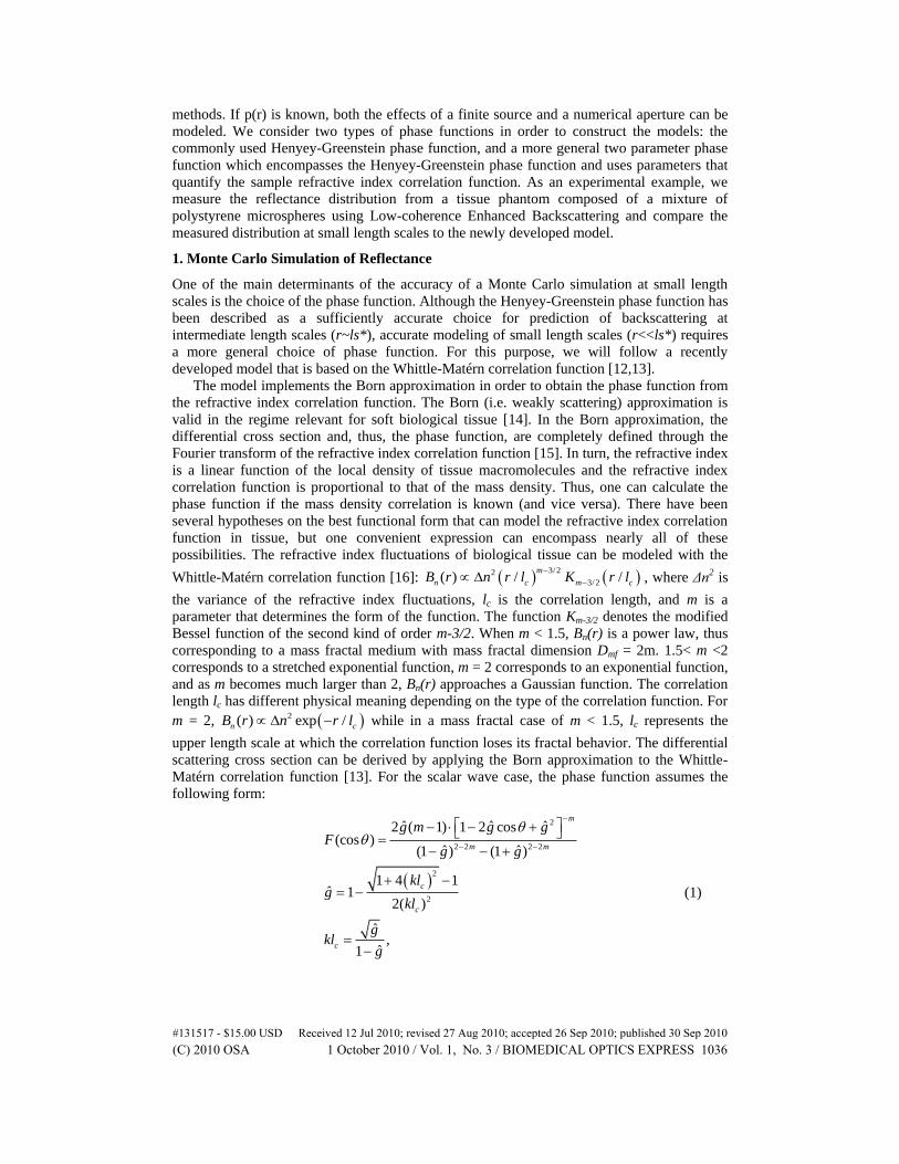

0 1 2 3 4
01
015
02
025
03
rls
P(r
ls)
g = 0
g = 07
g = 08
g = 09
0 025 05 075 1-005
0
005
01
rls
pro
babili
ty d
iffe
rence
Pg=07
- Pg=0
Pg=08
- Pg=0
Pg=09
- Pg=0
0 025 05 075 1-005
0
005
01
rls
pro
babili
ty d
iffe
rence
(P
g=07-P
g=0)c(07)
(Pg=08
-Pg=0
)c(08)
(Pg=09
-Pg=0
)c(09)
0 025 05 075 10
02
04
06
08
1
g
c(g
)
0 1 2 3 4
01
015
02
025
03
rls
P(r
ls)
g = 07
g = 08
g = 095
model
0 025 05 075 1
018
02
022
024
026
rls
P(r
ls)
g = 07
g = 08
g = 095
model
Equation
Simulation
a b c
Fig 2 Scaling relationships of P(rls) from the Henyey-Greenstein phase function (a) P(rls)
curves for varying values of g The curves have variations at rlslt1 and converge for larger
values of rls (b) Probability difference obtained by subtracting P(rls) for the isotropic case
(g = 0) from P(rls) of a given g (c) Probability difference curves for varying values of g with
the amplitude rescaled by a coefficient that depends only on g
We can therefore employ a predictive model of P(rls) that depends on just two
simulation results P(rls) for g = 0 and P(rls) for a particular ggt0 While any value of ggt0
can be used we use g = 09 in the following analysis for convenience (this results in accurate
prediction within the range of tissue anisotropy)
0 09 0( )
( )
g
b
P P c g P P
c g ag
(7)
where c(g) is an empirical model for the coefficients that multiply the difference term The
values of the constants a and b are approximately 1244 and 2338 respectively The shortened
notation Pg represents P(rls) for a given value of g (eg P09 = P(rls) for g = 09) The
values of c(g) were determined by fitting Monte Carlo results for a particular g to the
expression for Pg in Eq (7) The values of c(g) and the empirical model for c(g) are plotted in
Fig 3(a) We can understand the difference between P09 and P0 as the alteration in the
backscattering due to anisotropy As g increases the anisotropy contribution increases in
amplitude but retains a very similar radial shape This allows for a predictability of P(r) for
any value of g with only two reference P(r) distributions Fig 3(b) shows a comparison of the
Monte Carlo simulations and the model based on the difference relationship Fig 3(c) further
illustrates the details of the model fit at small values of rls Note that the fits for g = 0 and g
= 09 are not shown because the model and the Monte Carlo result are identical for those two
cases (c = 1 when g = 09 and c = 0 when g = 0) The model has excellent agreement for
values of g that are close to 09 but begins to deviate slightly at g = 07 As rls becomes
large all of the curves converge and the backscattering can be predicted with an isotropic
scattering model of equivalent ls
131517 - $1500 USD Received 12 Jul 2010 revised 27 Aug 2010 accepted 26 Sep 2010 published 30 Sep 2010(C) 2010 OSA 1 October 2010 Vol 1 No 3 BIOMEDICAL OPTICS EXPRESS 1039
0 1 2 3 4
01
015
02
025
03
rls
P(r
ls)
g = 0
g = 07
g = 08
g = 09
0 025 05 075 1-005
0
005
01
rls
pro
babili
ty d
iffe
rence
Pg=07
- Pg=0
Pg=08
- Pg=0
Pg=09
- Pg=0
0 025 05 075 1-005
0
005
01
rls
pro
babili
ty d
iffe
rence
(P
g=07-P
g=0)c(07)
(Pg=08
-Pg=0
)c(08)
(Pg=09
-Pg=0
)c(09)
0 025 05 075 10
02
04
06
08
1
g
c(g
)
0 1 2 3 4
01
015
02
025
03
rls
P(r
ls)
g = 07
g = 08
g = 095
model
0 025 05 075 1
018
02
022
024
026
rls
P(r
ls)
g = 07
g = 08
g = 095
model
Equation
Simulation
a b c
Fig 3 Backscattering model for P(rls) based on the Henyey-Greenstein phase function
utilizing the difference method (a) Value of amplitude coefficient as a function of g c(g) The
dots represent a least square fit to the Monte Carlo data and the solid line represents the model
for c(g) from Eq (7) The amplitude increases as a function of g follow a power law (b)
Comparison of Monte Carlo simulations (green red and purple curves) and model (black
curves) for three values of g g = 09 is not shown because the model and simulation are by
definition identical for that case (c) is a rescaled version of (b) shown for a smaller range of
rls
Another possible approach for predicting the backscattering signal at small radial
distances is through an implementation of principle component analysis (PCA) PCA is a
variance reduction technique that is often used to obtain dependencies when a large number of
variables are present The analysis typically involves mean-centering the data (ie subtracting
the mean from each variable) followed by a transformation which decomposes the data into
orthogonal components that explain the largest proportions of the variance within the data set
In order to apply this method to build a model of P(rls) we used each value in rls as an
input variable Instead of mean centering we subtracted the P(rls) curve for g = 0 The
effect of subtracting the isotropic P(rls) is similar to that of mean-centering but results in a
more predictable model that is independent of the particular reflectance distributions used in
the PCA analysis We then obtained a series of principle components and found that when the
first three components are used P(rls) can be predicted more accurately than the single-
component difference model described above The first three principle components (PC1-
PC3) predicted 99966 0027 0002 of the variance in the data respectively Based on
this model P(rls) can be predicted according to
0 1 2 3( ) 1 ( ) 2 ( ) 3g gP P c g PC c g PC c g PC (8)
where c1 c2 and c3 are the weights of the principle components We utilized a polynomial
equation to fit the weights with the order of the polynomial chosen such that the R2 coefficient
is greater than 099 Fig 4(a) shows a comparison of the principle component model with
Monte Carlo simulation results for three tissue-relevant values of g The rls axis is in log
scale showing that the model is in excellent agreement with the Monte Carlo simulations for
the entire simulated range of 0001lt rlslt10 Fig 4(b) shows the same comparison in linear
scale for the subdiffusion range of rls lt 1 again showing excellent agreement Fig 4(c)
shows the distributions of the three principle components that were used in the model Note
that the contribution of each successive component decreases with higher components being
noisier Fig 4(d) is a plot of the weights of the three components along with the polynomial
fits that are used for the predictive model
131517 - $1500 USD Received 12 Jul 2010 revised 27 Aug 2010 accepted 26 Sep 2010 published 30 Sep 2010(C) 2010 OSA 1 October 2010 Vol 1 No 3 BIOMEDICAL OPTICS EXPRESS 1040
a b
c d
C1 fit
C2 fit
C3 fit
C1
C2
C3
Fig 4 Backscattering model for the Henyey-Greenstein case utilizing principle component
analysis method (a) Semi-log plot of Monte Carlo simulations and the PCA model for three
values of g (b) Comparison of PCA model and Monte Carlo simulation for rls lt 1 (c) Semi-
log plot of the three principle components Note that higher principle components have less
amplitude and contribute less to P(rls) prediction (d) Plot of coefficients that multiply the
principle components and their polynomial fits used to obtain the predictive model
3 Model of Reflectance Whittle-Mateacutern Phase Function
To obtain a generalized model for reflectance based on the Whittle-Mateacutern phase function we
simulated P(rls) distributions for varying values of g and m In Fig 5(a) P(rls) curves for
four values of m are shown with a constant anisotropy factor of g = 09 The isotropic
component is subtracted from these curves in Fig 5(b) From Fig 5(b) it is apparent that a
simple scaling in amplitude cannot account for the difference between these curves There is
an m-dependent alteration in the shape of the non-diffuse component of the curves However
for a given value of m changes in g only alter the amplitude of the non-diffuse component
[Fig 5(c)] Therefore it is clear that another component needs to be introduced that can
account for the alterations in the shape of P(rls) due to varying m We can extend the
difference model developed for the Henyey-Greenstein phase function (m = 15) discussed in
the previous section by defining a second difference component that is calculated by
subtracting the isotropic probability from P(rls) for g = 09 and a particular m In our
analysis we chose m = 101 This value of m was chosen because the shape of P(rls)
becomes dramatically altered as m approaches 1 The shapes of the two difference
components are compared in
Fig 5(d) P(rls) can then be predicted according to a two-component model
0 1 1 2 2
1 09 15 0
2 09 101 0
( ) ( )g m g
g m g
g m g
P P c g m P c g m P
P P P
P P P
(9)
The coefficients c1 and c2 vary smoothly and continuously with g and m These
coefficients can be fit to a variety of functions depending on the desired simplicity and
accuracy of the model We fit these coefficients to a third order polynomial in two dimensions
described by Eq (10)
2 2 3 3 2 2 i i i i i i i i i i ic a b x c y d x e y f x g y h xy i x y j xy (10)
131517 - $1500 USD Received 12 Jul 2010 revised 27 Aug 2010 accepted 26 Sep 2010 published 30 Sep 2010(C) 2010 OSA 1 October 2010 Vol 1 No 3 BIOMEDICAL OPTICS EXPRESS 1041
where x = ln(m) and y = 1(1-g) The constants a ndash j are supplied in Table 1 These constants
were optimized to obtain a minimized error for g06
a b
c d
Fig 5 P(rls) distributions for the generalized Whittle-Mateacutern phase function (a) P(rls)
dependence on m for g = 09 The shape of the P(rls) gradually changes with varying m (b)
Probability difference between P(rls) curves and the isotropic P(rls) for g = 09 and varying
m Unlike changes in g alterations in m cannot be accounted for by a simple scaling of the
amplitude of the probability difference curves (d) Probability difference curves for various
values of g and m = 18 The probability difference only changes in amplitude for a constant m
and varying g (d) The two probability difference curves used to model P(rls) from Eq (9)
Alternatively a principle component model can also be adopted similar to the one
described by Eq (8) except that the coefficients c1 c2 and c3 each vary as a function of g and
m in the generalized model The variation of these coefficients is also smooth and continuous
and can be fit to a polynomial equation based model such as the one in Eq (10) Fig 6(a)
shows a comparison of the difference model (PΔ model) for the Whittle-Mateacutern phase
function with Monte Carlo results for varying values of m and a constant g of 09 The
agreement is excellent although the error slightly increases for larger values of m The
agreement is improved for the PCA based model shown in Fig 6(b) The error is quantified
for the entire range of g and m for the PΔ and PCA models in Fig 6(c) and Fig 6(d)
respectively Although the equations were optimized for g06 the average error for rls
between 0 and 1 is less than 2 for the entire range of g and m values that were evaluated
The error was less than 1 for all values of m and biologically relevant anisotropy factors
(g06) The PCA model had less error than the PΔ model for this biologically relevant
anisotropy range
131517 - $1500 USD Received 12 Jul 2010 revised 27 Aug 2010 accepted 26 Sep 2010 published 30 Sep 2010(C) 2010 OSA 1 October 2010 Vol 1 No 3 BIOMEDICAL OPTICS EXPRESS 1042
Table 1 Values of constants from coefficients for PΔ model [Eq (9)]
Constant C1 C2
a 029773 0064755 b 011547 046123
c 0068216 015039
d 13086 15305
e 00045095 00049453
f 11378 10031
g 74495105 39844105
h 025636 037841
i 0047610 013420 j 00071922 00082885
a b
c d
a b
c d
Fig 6 Evaluation of P(rls) predictive model accuracy (a) PΔ model for P(rls) (lines)
compared to Monte Carlo data (points) for varying values of m and g = 09 (b) PCA model for
P(rls) (lines) compared to Monte Carlo data (points) for varying values of m and g = 09 (c)
Average error of PΔ model as a function of g for rlslt1 (d) Average error of PCA model as a
function of g for rlslt1
It is important to point out that the presented model does not incorporate absorption
However the absorption is expected to be much smaller at small radial distances because the
path length and the exit radius of a ray traversing a turbid medium are known to be well
correlated To estimate the range of absorption under which the presented models are
accurate we performed three Monte Carlo simulations with identical optical properties but a
varying absorption coefficient In this case each of the backscattering distributions was
normalized by the total backscattering reflectance that would be present in the absence of
absorption The resulting reflectance distributions are shown in Fig 7 Absorption primarily
alters the intensity of backscattering at larger radial distances and has a minimal effect at r ltlt
la where la = 1microa This can be reasoned from the Beer-Lambert law and the fact that the path
lengths contributing to backscattering at small radial distances are small For larger radial
distances the path length becomes longer and the effect of absorption becomes substantial
Therefore one can also incorporate traditional diffusion approximation models of absorption
in order to quantify the backscattering contribution In this case the isotropic scattering
131517 - $1500 USD Received 12 Jul 2010 revised 27 Aug 2010 accepted 26 Sep 2010 published 30 Sep 2010(C) 2010 OSA 1 October 2010 Vol 1 No 3 BIOMEDICAL OPTICS EXPRESS 1043
portion [Pg = 0 from Eq (7) to (9)] can be modeled with standard diffusion approximation
equations for reflectance [1819]
0 50 100 150 20005
1
15
2
25
3
35
4x 10
-3
r (m)
P(r
)
a = 0
a = 1 cm-1
a = 10 cm-1
Fig 7 P(r) for varying microa The scattering properties of all three simulations were maintained at
micros = 100 cm1 g = 09 and m = 16 Absorption has a minimal effect at small radial distances
because of the short path lengths involved
4 Experimental Measurement of P(r) from Tissue Phantom
As an illustrative example of an application of the presented models we utilized Low-
Coherence Enhanced Backscattering (LEBS) to measure P(r) for rltls The experimental
system used for the measurements has been described elsewhere and validated with P(r)
measurements and simulations of mono-dispersed polystyrene microspheres in water [20] A
phantom was constructed from a mixture of polystyrene microsphere suspensions in order to
mimic the Whittle-Mateacutern phase function The proportions of microsphere sizes were
determined by fitting three commonly available sizes such that the final phase function
matched closely to the Whittle-Mateacutern phase function Microspheres that were sized 026
052 and 10microm were mixed in respective volume proportions of 10207 When the
suspension is dilute and the scattering is weak the weighted average of the phase functions
(with the weights being proportional to the concentration and the scattering cross section of
the microspheres) results in the effective phase function of the scattering medium The phase
functions for microsphere particles and their scattering cross sections were calculated with
Mie theory The phase function fit was further improved by raising the refractive index of the
medium to 134 with glycerol A Whittle-Mateacutern phase function with an m of 16 and g of 08
is compared to the resulting phase function obtained from the microsphere mixture in
Fig 8(a) In principle the agreement may further be improved by using a larger variety of
sphere sizes We then obtained measurements for the unpolarized P(r) by measuring the
unpolarized LEBS signal and dividing the Fourier transform of the signal by the coherence
function [20] In this example we approximated the coherence function to be the shape of an
idealized first order Bessel function of the first kind with a spatial coherence length of 110microm
as calculated from the van-Cittert-Zernike theorem We accounted for the decrease in the
enhancement factor due to the contribution of orthogonally polarized light by assuming that
unpolarized light is an equal mixture of the two orthogonal polarization states This results in
an enhancement of 175 when dividing by the incoherent baseline or 075 when the baseline
is subtracted [21] We also accounted for the discrepancy between Monte Carlo and
experimental measurement that was observed in earlier work with a factor of 05 [20] These
constants were determined to be accurate by measuring P(r) from mono-disperse microsphere
suspensions with varying sizes and comparing to Monte Carlo simulations that track
polarization and utilized the Mie phase function The experimentally measured P(r) and the
P(r) obtained from the PCA model were in excellent agreement for r ltlt ls [Fig 8(b)] with
an average error of 71 for the range shown It is interesting to note that the noise level from
131517 - $1500 USD Received 12 Jul 2010 revised 27 Aug 2010 accepted 26 Sep 2010 published 30 Sep 2010(C) 2010 OSA 1 October 2010 Vol 1 No 3 BIOMEDICAL OPTICS EXPRESS 1044
the experimental measurement in Fig 8(b) varies with the radial position The LEBS method
measures the two-dimensional quantity p(xy) via a two-dimensional Fourier transform The
higher noise level at small radii is a result of the decreased number of pixel elements that
contribute to the summation over the polar angle As r increases the noise level decreases
until the coherence function begins to approach small values at which point the noise level
quickly rises due to the division of two numbers that have values near 0
-150 -100 -50 0 50 100 15010
-2
10-1
100
101
Angle (degrees)
F(
)
W-M
Spheres
0 50 100 150 200 250 3002
3
4
5x 10
-4
r (m)
P(r
)
Monte Carlo
Experiment
Model
a b
Fig 8 Tissue phantom for experimental measurement of P(r) (a) Comparison of the Whittle-
Mateacutern phase function (m = 16 and g = 08) with the fit obtained from a mixture of
microspheres of three sizes (b) Resulting P(r) experimentally measured with LEBS compared
with P(r) obtained with the PCA based model and a Monte Carlo simulation An ls of 800μm
determined from the Mie theory calculation was used for the model and Monte Carlo curve
The experimental LEBS measurement was scaled by the 075 factor to account for unpolarized
light and the empirical 05 factor determined from microsphere studies in prior work [20] to
account for the difference observed between LEBS and Monte Carlo (see text) The average
error between the experimentally measured P(r) and the model was 71
5 Conclusions
We have presented two models capable of predicting P(rls) for the entire range of rls
Each model was applied to predicting reflectance from random media with a Henyey-
Greenstein phase function and a generalized phase function that is derived from the Whittle-
Mateacutern correlation function The presented models consist of an empirical equation that
quantifies the difference between the isotropic case of g = 0 and non-isotropic cases of ggt0
This difference is predicted with two methods the PΔ method and the PCA method The PΔ
method is based on the observation that these differences only scale in amplitude as g is
varied [Fig 2(c)] and do not change their shape Although the shape of the radial dependence
of this anisotropy contribution depends on m it can be predicted with a linear combination of
two difference terms [Eq (9)] The PΔ model results in accurate prediction for the Henyey-
Greenstein case [Fig 3(c)] and the generalized Whittle-Mateacutern phase case [Fig 6(a)] The
PΔ(rls) terms used in this model can be thought of as the anisotropic contribution to
P(rls) with the amplitude of these terms being related to the anisotropy factor
The PCA method uses a similar idea as the PΔ method in that the anisotropy contribution
is quantified The advantage of the PCA method is that it decomposes the radial contributions
into orthogonal principle components that explain the largest variations in the Monte Carlo
data Although in principle using more principle components results in a more accurate
prediction of the data in practice accurate prediction also relies on being able to model the
coefficients associated with the principle components The dependence of these coefficients
with the phase function properties become increasingly complicated for higher principle
components [Fig 4(d)] and therefore the model that fits these coefficients requires increasing
complexity We used a polynomial model for the Henyey-Greenstein phase function and a
two-dimensional cubic [Eq (10)] for the Whittle-Mateacutern phase function This resulted in
excellent agreement for the biological tissue regime where ggt06 [Fig 4(a) and Fig 6(d)]
The results of the fits can potentially be improved by implementing more principle
131517 - $1500 USD Received 12 Jul 2010 revised 27 Aug 2010 accepted 26 Sep 2010 published 30 Sep 2010(C) 2010 OSA 1 October 2010 Vol 1 No 3 BIOMEDICAL OPTICS EXPRESS 1045
components increasing the accuracy of the model fit to the coefficients or fitting to a smaller
range of optical properties That said the error for the model applied to biologically relevant
optical properties (gge06 and 1ltmlt2) was less than 1 The same procedure that was
presented here can be used for modeling other ranges of g and m in order to obtain improved
accuracy
As mentioned in section 3 absorption is not included in the models described in this
manuscript However in biological tissue absorption varies dramatically with wavelength
and is typically small for λgt600nm Therefore the technique described here can be utilized to
measure scattering properties in the non-absorbing wavelength regions Absorption can then
be characterized by understanding the path length distribution for varying optical properties
and measuring the backscattering for varying wavelengths From Fig 7 we can conclude that
absorption primarily alters the intensity of backscattering at larger radial distances and has a
minimal effect at r ltlt la This is due to shorter path lengths at smaller radial distances
resulting in less attenuation of the scattered rays (The Beer-Lambert law) In cases where
absorption cannot be neglected a traditional diffusion approximation model of absorption in
order to quantify the backscattering contribution can be used In this case the isotropic
scattering portion [Pg = 0 from Eq (7) to (9)] can be modeled with standard diffusion
approximation equations for reflectance [1819]
In conclusion the models presented in this work allow for accurate prediction of the
impulse response function P(r) to a random medium with a tissue-relevant range of optical
properties and without the need for performing a large number of Monte Carlo simulations
Only three simulations are required including a simulation for isotropic scattering and two
simulations for anisotropic scattering (g = 09 with m of 15 and 101) A Henyey-Greenstein
based P(r) model is simpler in that it only requires two Monte Carlo simulations however it
may not be as comprehensive of a model for tissue characterization Finally we presented a
methodology for obtaining phantoms that have the potential to closely mimic optical
properties of tissue including the backscattering at small length-scales The ability to predict
the backscattering distribution at subdiffusion length scales holds promise for using
techniques such as LEBS to measure optical properties of tissue (such as g m and ls) by
measuring P(r) These results may also allow for faster simpler and more accurate solutions
to the inverse problem of measuring optical properties from tissue by providing an alternative
for existing inverse Monte Carlo methods [56112223] The three simulation and coefficient
equations necessary for predicting P(r) will be made available online for public use
Furthermore there are currently no existing empirical or theoretical models that allow for the
prediction of the backscattered light at subdiffusion length scales without the need for
performing repetitive and time intensive Monte Carlo simulations The high degree of
accuracy of the presented models and experimental illustration of a P(r) measurement from
the Whittle-Mateacutern phase function at rltls indicate that the presented models and
experimental phantom will be useful for characterizing the optical properties of biological
samples
Acknowledgements
This work was supported by National Institutes of Health (NIH) grants R01 CA128641 R01
CA109861 R01 EB003682 and R01 CA118794
131517 - $1500 USD Received 12 Jul 2010 revised 27 Aug 2010 accepted 26 Sep 2010 published 30 Sep 2010(C) 2010 OSA 1 October 2010 Vol 1 No 3 BIOMEDICAL OPTICS EXPRESS 1046
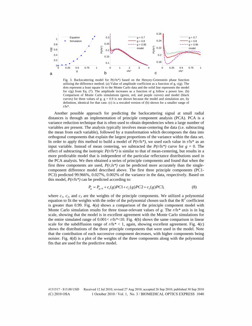
0 1 2 3 4
01
015
02
025
03
rls
P(r
ls)
g = 0
g = 07
g = 08
g = 09
0 025 05 075 1-005
0
005
01
rls
pro
babili
ty d
iffe
rence
Pg=07
- Pg=0
Pg=08
- Pg=0
Pg=09
- Pg=0
0 025 05 075 1-005
0
005
01
rls
pro
babili
ty d
iffe
rence
(P
g=07-P
g=0)c(07)
(Pg=08
-Pg=0
)c(08)
(Pg=09
-Pg=0
)c(09)
0 025 05 075 10
02
04
06
08
1
g
c(g
)
0 1 2 3 4
01
015
02
025
03
rls
P(r
ls)
g = 07
g = 08
g = 095
model
0 025 05 075 1
018
02
022
024
026
rls
P(r
ls)
g = 07
g = 08
g = 095
model
Equation
Simulation
a b c
Fig 3 Backscattering model for P(rls) based on the Henyey-Greenstein phase function
utilizing the difference method (a) Value of amplitude coefficient as a function of g c(g) The
dots represent a least square fit to the Monte Carlo data and the solid line represents the model
for c(g) from Eq (7) The amplitude increases as a function of g follow a power law (b)
Comparison of Monte Carlo simulations (green red and purple curves) and model (black
curves) for three values of g g = 09 is not shown because the model and simulation are by
definition identical for that case (c) is a rescaled version of (b) shown for a smaller range of
rls
Another possible approach for predicting the backscattering signal at small radial
distances is through an implementation of principle component analysis (PCA) PCA is a
variance reduction technique that is often used to obtain dependencies when a large number of
variables are present The analysis typically involves mean-centering the data (ie subtracting
the mean from each variable) followed by a transformation which decomposes the data into
orthogonal components that explain the largest proportions of the variance within the data set
In order to apply this method to build a model of P(rls) we used each value in rls as an
input variable Instead of mean centering we subtracted the P(rls) curve for g = 0 The
effect of subtracting the isotropic P(rls) is similar to that of mean-centering but results in a
more predictable model that is independent of the particular reflectance distributions used in
the PCA analysis We then obtained a series of principle components and found that when the
first three components are used P(rls) can be predicted more accurately than the single-
component difference model described above The first three principle components (PC1-
PC3) predicted 99966 0027 0002 of the variance in the data respectively Based on
this model P(rls) can be predicted according to
0 1 2 3( ) 1 ( ) 2 ( ) 3g gP P c g PC c g PC c g PC (8)
where c1 c2 and c3 are the weights of the principle components We utilized a polynomial
equation to fit the weights with the order of the polynomial chosen such that the R2 coefficient
is greater than 099 Fig 4(a) shows a comparison of the principle component model with
Monte Carlo simulation results for three tissue-relevant values of g The rls axis is in log
scale showing that the model is in excellent agreement with the Monte Carlo simulations for
the entire simulated range of 0001lt rlslt10 Fig 4(b) shows the same comparison in linear
scale for the subdiffusion range of rls lt 1 again showing excellent agreement Fig 4(c)
shows the distributions of the three principle components that were used in the model Note
that the contribution of each successive component decreases with higher components being
noisier Fig 4(d) is a plot of the weights of the three components along with the polynomial
fits that are used for the predictive model
131517 - $1500 USD Received 12 Jul 2010 revised 27 Aug 2010 accepted 26 Sep 2010 published 30 Sep 2010(C) 2010 OSA 1 October 2010 Vol 1 No 3 BIOMEDICAL OPTICS EXPRESS 1040
a b
c d
C1 fit
C2 fit
C3 fit
C1
C2
C3
Fig 4 Backscattering model for the Henyey-Greenstein case utilizing principle component
analysis method (a) Semi-log plot of Monte Carlo simulations and the PCA model for three
values of g (b) Comparison of PCA model and Monte Carlo simulation for rls lt 1 (c) Semi-
log plot of the three principle components Note that higher principle components have less
amplitude and contribute less to P(rls) prediction (d) Plot of coefficients that multiply the
principle components and their polynomial fits used to obtain the predictive model
3 Model of Reflectance Whittle-Mateacutern Phase Function
To obtain a generalized model for reflectance based on the Whittle-Mateacutern phase function we
simulated P(rls) distributions for varying values of g and m In Fig 5(a) P(rls) curves for
four values of m are shown with a constant anisotropy factor of g = 09 The isotropic
component is subtracted from these curves in Fig 5(b) From Fig 5(b) it is apparent that a
simple scaling in amplitude cannot account for the difference between these curves There is
an m-dependent alteration in the shape of the non-diffuse component of the curves However
for a given value of m changes in g only alter the amplitude of the non-diffuse component
[Fig 5(c)] Therefore it is clear that another component needs to be introduced that can
account for the alterations in the shape of P(rls) due to varying m We can extend the
difference model developed for the Henyey-Greenstein phase function (m = 15) discussed in
the previous section by defining a second difference component that is calculated by
subtracting the isotropic probability from P(rls) for g = 09 and a particular m In our
analysis we chose m = 101 This value of m was chosen because the shape of P(rls)
becomes dramatically altered as m approaches 1 The shapes of the two difference
components are compared in
Fig 5(d) P(rls) can then be predicted according to a two-component model
0 1 1 2 2
1 09 15 0
2 09 101 0
( ) ( )g m g
g m g
g m g
P P c g m P c g m P
P P P
P P P
(9)
The coefficients c1 and c2 vary smoothly and continuously with g and m These
coefficients can be fit to a variety of functions depending on the desired simplicity and
accuracy of the model We fit these coefficients to a third order polynomial in two dimensions
described by Eq (10)
2 2 3 3 2 2 i i i i i i i i i i ic a b x c y d x e y f x g y h xy i x y j xy (10)
131517 - $1500 USD Received 12 Jul 2010 revised 27 Aug 2010 accepted 26 Sep 2010 published 30 Sep 2010(C) 2010 OSA 1 October 2010 Vol 1 No 3 BIOMEDICAL OPTICS EXPRESS 1041
where x = ln(m) and y = 1(1-g) The constants a ndash j are supplied in Table 1 These constants
were optimized to obtain a minimized error for g06
a b
c d
Fig 5 P(rls) distributions for the generalized Whittle-Mateacutern phase function (a) P(rls)
dependence on m for g = 09 The shape of the P(rls) gradually changes with varying m (b)
Probability difference between P(rls) curves and the isotropic P(rls) for g = 09 and varying
m Unlike changes in g alterations in m cannot be accounted for by a simple scaling of the
amplitude of the probability difference curves (d) Probability difference curves for various
values of g and m = 18 The probability difference only changes in amplitude for a constant m
and varying g (d) The two probability difference curves used to model P(rls) from Eq (9)
Alternatively a principle component model can also be adopted similar to the one
described by Eq (8) except that the coefficients c1 c2 and c3 each vary as a function of g and
m in the generalized model The variation of these coefficients is also smooth and continuous
and can be fit to a polynomial equation based model such as the one in Eq (10) Fig 6(a)
shows a comparison of the difference model (PΔ model) for the Whittle-Mateacutern phase
function with Monte Carlo results for varying values of m and a constant g of 09 The
agreement is excellent although the error slightly increases for larger values of m The
agreement is improved for the PCA based model shown in Fig 6(b) The error is quantified
for the entire range of g and m for the PΔ and PCA models in Fig 6(c) and Fig 6(d)
respectively Although the equations were optimized for g06 the average error for rls
between 0 and 1 is less than 2 for the entire range of g and m values that were evaluated
The error was less than 1 for all values of m and biologically relevant anisotropy factors
(g06) The PCA model had less error than the PΔ model for this biologically relevant
anisotropy range
131517 - $1500 USD Received 12 Jul 2010 revised 27 Aug 2010 accepted 26 Sep 2010 published 30 Sep 2010(C) 2010 OSA 1 October 2010 Vol 1 No 3 BIOMEDICAL OPTICS EXPRESS 1042
Table 1 Values of constants from coefficients for PΔ model [Eq (9)]
Constant C1 C2
a 029773 0064755 b 011547 046123
c 0068216 015039
d 13086 15305
e 00045095 00049453
f 11378 10031
g 74495105 39844105
h 025636 037841
i 0047610 013420 j 00071922 00082885
a b
c d
a b
c d
Fig 6 Evaluation of P(rls) predictive model accuracy (a) PΔ model for P(rls) (lines)
compared to Monte Carlo data (points) for varying values of m and g = 09 (b) PCA model for
P(rls) (lines) compared to Monte Carlo data (points) for varying values of m and g = 09 (c)
Average error of PΔ model as a function of g for rlslt1 (d) Average error of PCA model as a
function of g for rlslt1
It is important to point out that the presented model does not incorporate absorption
However the absorption is expected to be much smaller at small radial distances because the
path length and the exit radius of a ray traversing a turbid medium are known to be well
correlated To estimate the range of absorption under which the presented models are
accurate we performed three Monte Carlo simulations with identical optical properties but a
varying absorption coefficient In this case each of the backscattering distributions was
normalized by the total backscattering reflectance that would be present in the absence of
absorption The resulting reflectance distributions are shown in Fig 7 Absorption primarily
alters the intensity of backscattering at larger radial distances and has a minimal effect at r ltlt
la where la = 1microa This can be reasoned from the Beer-Lambert law and the fact that the path
lengths contributing to backscattering at small radial distances are small For larger radial
distances the path length becomes longer and the effect of absorption becomes substantial
Therefore one can also incorporate traditional diffusion approximation models of absorption
in order to quantify the backscattering contribution In this case the isotropic scattering
131517 - $1500 USD Received 12 Jul 2010 revised 27 Aug 2010 accepted 26 Sep 2010 published 30 Sep 2010(C) 2010 OSA 1 October 2010 Vol 1 No 3 BIOMEDICAL OPTICS EXPRESS 1043
portion [Pg = 0 from Eq (7) to (9)] can be modeled with standard diffusion approximation
equations for reflectance [1819]
0 50 100 150 20005
1
15
2
25
3
35
4x 10
-3
r (m)
P(r
)
a = 0
a = 1 cm-1
a = 10 cm-1
Fig 7 P(r) for varying microa The scattering properties of all three simulations were maintained at
micros = 100 cm1 g = 09 and m = 16 Absorption has a minimal effect at small radial distances
because of the short path lengths involved
4 Experimental Measurement of P(r) from Tissue Phantom
As an illustrative example of an application of the presented models we utilized Low-
Coherence Enhanced Backscattering (LEBS) to measure P(r) for rltls The experimental
system used for the measurements has been described elsewhere and validated with P(r)
measurements and simulations of mono-dispersed polystyrene microspheres in water [20] A
phantom was constructed from a mixture of polystyrene microsphere suspensions in order to
mimic the Whittle-Mateacutern phase function The proportions of microsphere sizes were
determined by fitting three commonly available sizes such that the final phase function
matched closely to the Whittle-Mateacutern phase function Microspheres that were sized 026
052 and 10microm were mixed in respective volume proportions of 10207 When the
suspension is dilute and the scattering is weak the weighted average of the phase functions
(with the weights being proportional to the concentration and the scattering cross section of
the microspheres) results in the effective phase function of the scattering medium The phase
functions for microsphere particles and their scattering cross sections were calculated with
Mie theory The phase function fit was further improved by raising the refractive index of the
medium to 134 with glycerol A Whittle-Mateacutern phase function with an m of 16 and g of 08
is compared to the resulting phase function obtained from the microsphere mixture in
Fig 8(a) In principle the agreement may further be improved by using a larger variety of
sphere sizes We then obtained measurements for the unpolarized P(r) by measuring the
unpolarized LEBS signal and dividing the Fourier transform of the signal by the coherence
function [20] In this example we approximated the coherence function to be the shape of an
idealized first order Bessel function of the first kind with a spatial coherence length of 110microm
as calculated from the van-Cittert-Zernike theorem We accounted for the decrease in the
enhancement factor due to the contribution of orthogonally polarized light by assuming that
unpolarized light is an equal mixture of the two orthogonal polarization states This results in
an enhancement of 175 when dividing by the incoherent baseline or 075 when the baseline
is subtracted [21] We also accounted for the discrepancy between Monte Carlo and
experimental measurement that was observed in earlier work with a factor of 05 [20] These
constants were determined to be accurate by measuring P(r) from mono-disperse microsphere
suspensions with varying sizes and comparing to Monte Carlo simulations that track
polarization and utilized the Mie phase function The experimentally measured P(r) and the
P(r) obtained from the PCA model were in excellent agreement for r ltlt ls [Fig 8(b)] with
an average error of 71 for the range shown It is interesting to note that the noise level from
131517 - $1500 USD Received 12 Jul 2010 revised 27 Aug 2010 accepted 26 Sep 2010 published 30 Sep 2010(C) 2010 OSA 1 October 2010 Vol 1 No 3 BIOMEDICAL OPTICS EXPRESS 1044
the experimental measurement in Fig 8(b) varies with the radial position The LEBS method
measures the two-dimensional quantity p(xy) via a two-dimensional Fourier transform The
higher noise level at small radii is a result of the decreased number of pixel elements that
contribute to the summation over the polar angle As r increases the noise level decreases
until the coherence function begins to approach small values at which point the noise level
quickly rises due to the division of two numbers that have values near 0
-150 -100 -50 0 50 100 15010
-2
10-1
100
101
Angle (degrees)
F(
)
W-M
Spheres
0 50 100 150 200 250 3002
3
4
5x 10
-4
r (m)
P(r
)
Monte Carlo
Experiment
Model
a b
Fig 8 Tissue phantom for experimental measurement of P(r) (a) Comparison of the Whittle-
Mateacutern phase function (m = 16 and g = 08) with the fit obtained from a mixture of
microspheres of three sizes (b) Resulting P(r) experimentally measured with LEBS compared
with P(r) obtained with the PCA based model and a Monte Carlo simulation An ls of 800μm
determined from the Mie theory calculation was used for the model and Monte Carlo curve
The experimental LEBS measurement was scaled by the 075 factor to account for unpolarized
light and the empirical 05 factor determined from microsphere studies in prior work [20] to
account for the difference observed between LEBS and Monte Carlo (see text) The average
error between the experimentally measured P(r) and the model was 71
5 Conclusions
We have presented two models capable of predicting P(rls) for the entire range of rls
Each model was applied to predicting reflectance from random media with a Henyey-
Greenstein phase function and a generalized phase function that is derived from the Whittle-
Mateacutern correlation function The presented models consist of an empirical equation that
quantifies the difference between the isotropic case of g = 0 and non-isotropic cases of ggt0
This difference is predicted with two methods the PΔ method and the PCA method The PΔ
method is based on the observation that these differences only scale in amplitude as g is
varied [Fig 2(c)] and do not change their shape Although the shape of the radial dependence
of this anisotropy contribution depends on m it can be predicted with a linear combination of
two difference terms [Eq (9)] The PΔ model results in accurate prediction for the Henyey-
Greenstein case [Fig 3(c)] and the generalized Whittle-Mateacutern phase case [Fig 6(a)] The
PΔ(rls) terms used in this model can be thought of as the anisotropic contribution to
P(rls) with the amplitude of these terms being related to the anisotropy factor
The PCA method uses a similar idea as the PΔ method in that the anisotropy contribution
is quantified The advantage of the PCA method is that it decomposes the radial contributions
into orthogonal principle components that explain the largest variations in the Monte Carlo
data Although in principle using more principle components results in a more accurate
prediction of the data in practice accurate prediction also relies on being able to model the
coefficients associated with the principle components The dependence of these coefficients
with the phase function properties become increasingly complicated for higher principle
components [Fig 4(d)] and therefore the model that fits these coefficients requires increasing
complexity We used a polynomial model for the Henyey-Greenstein phase function and a
two-dimensional cubic [Eq (10)] for the Whittle-Mateacutern phase function This resulted in
excellent agreement for the biological tissue regime where ggt06 [Fig 4(a) and Fig 6(d)]
The results of the fits can potentially be improved by implementing more principle
131517 - $1500 USD Received 12 Jul 2010 revised 27 Aug 2010 accepted 26 Sep 2010 published 30 Sep 2010(C) 2010 OSA 1 October 2010 Vol 1 No 3 BIOMEDICAL OPTICS EXPRESS 1045
components increasing the accuracy of the model fit to the coefficients or fitting to a smaller
range of optical properties That said the error for the model applied to biologically relevant
optical properties (gge06 and 1ltmlt2) was less than 1 The same procedure that was
presented here can be used for modeling other ranges of g and m in order to obtain improved
accuracy
As mentioned in section 3 absorption is not included in the models described in this
manuscript However in biological tissue absorption varies dramatically with wavelength
and is typically small for λgt600nm Therefore the technique described here can be utilized to
measure scattering properties in the non-absorbing wavelength regions Absorption can then
be characterized by understanding the path length distribution for varying optical properties
and measuring the backscattering for varying wavelengths From Fig 7 we can conclude that
absorption primarily alters the intensity of backscattering at larger radial distances and has a
minimal effect at r ltlt la This is due to shorter path lengths at smaller radial distances
resulting in less attenuation of the scattered rays (The Beer-Lambert law) In cases where
absorption cannot be neglected a traditional diffusion approximation model of absorption in
order to quantify the backscattering contribution can be used In this case the isotropic
scattering portion [Pg = 0 from Eq (7) to (9)] can be modeled with standard diffusion
approximation equations for reflectance [1819]
In conclusion the models presented in this work allow for accurate prediction of the
impulse response function P(r) to a random medium with a tissue-relevant range of optical
properties and without the need for performing a large number of Monte Carlo simulations
Only three simulations are required including a simulation for isotropic scattering and two
simulations for anisotropic scattering (g = 09 with m of 15 and 101) A Henyey-Greenstein
based P(r) model is simpler in that it only requires two Monte Carlo simulations however it
may not be as comprehensive of a model for tissue characterization Finally we presented a
methodology for obtaining phantoms that have the potential to closely mimic optical
properties of tissue including the backscattering at small length-scales The ability to predict
the backscattering distribution at subdiffusion length scales holds promise for using
techniques such as LEBS to measure optical properties of tissue (such as g m and ls) by
measuring P(r) These results may also allow for faster simpler and more accurate solutions
to the inverse problem of measuring optical properties from tissue by providing an alternative
for existing inverse Monte Carlo methods [56112223] The three simulation and coefficient
equations necessary for predicting P(r) will be made available online for public use
Furthermore there are currently no existing empirical or theoretical models that allow for the
prediction of the backscattered light at subdiffusion length scales without the need for
performing repetitive and time intensive Monte Carlo simulations The high degree of
accuracy of the presented models and experimental illustration of a P(r) measurement from
the Whittle-Mateacutern phase function at rltls indicate that the presented models and
experimental phantom will be useful for characterizing the optical properties of biological
samples
Acknowledgements
This work was supported by National Institutes of Health (NIH) grants R01 CA128641 R01
CA109861 R01 EB003682 and R01 CA118794
131517 - $1500 USD Received 12 Jul 2010 revised 27 Aug 2010 accepted 26 Sep 2010 published 30 Sep 2010(C) 2010 OSA 1 October 2010 Vol 1 No 3 BIOMEDICAL OPTICS EXPRESS 1046
a b
c d
C1 fit
C2 fit
C3 fit
C1
C2
C3
Fig 4 Backscattering model for the Henyey-Greenstein case utilizing principle component
analysis method (a) Semi-log plot of Monte Carlo simulations and the PCA model for three
values of g (b) Comparison of PCA model and Monte Carlo simulation for rls lt 1 (c) Semi-
log plot of the three principle components Note that higher principle components have less
amplitude and contribute less to P(rls) prediction (d) Plot of coefficients that multiply the
principle components and their polynomial fits used to obtain the predictive model
3 Model of Reflectance Whittle-Mateacutern Phase Function
To obtain a generalized model for reflectance based on the Whittle-Mateacutern phase function we
simulated P(rls) distributions for varying values of g and m In Fig 5(a) P(rls) curves for
four values of m are shown with a constant anisotropy factor of g = 09 The isotropic
component is subtracted from these curves in Fig 5(b) From Fig 5(b) it is apparent that a
simple scaling in amplitude cannot account for the difference between these curves There is
an m-dependent alteration in the shape of the non-diffuse component of the curves However
for a given value of m changes in g only alter the amplitude of the non-diffuse component
[Fig 5(c)] Therefore it is clear that another component needs to be introduced that can
account for the alterations in the shape of P(rls) due to varying m We can extend the
difference model developed for the Henyey-Greenstein phase function (m = 15) discussed in
the previous section by defining a second difference component that is calculated by
subtracting the isotropic probability from P(rls) for g = 09 and a particular m In our
analysis we chose m = 101 This value of m was chosen because the shape of P(rls)
becomes dramatically altered as m approaches 1 The shapes of the two difference
components are compared in
Fig 5(d) P(rls) can then be predicted according to a two-component model
0 1 1 2 2
1 09 15 0
2 09 101 0
( ) ( )g m g
g m g
g m g
P P c g m P c g m P
P P P
P P P
(9)
The coefficients c1 and c2 vary smoothly and continuously with g and m These
coefficients can be fit to a variety of functions depending on the desired simplicity and
accuracy of the model We fit these coefficients to a third order polynomial in two dimensions
described by Eq (10)
2 2 3 3 2 2 i i i i i i i i i i ic a b x c y d x e y f x g y h xy i x y j xy (10)
131517 - $1500 USD Received 12 Jul 2010 revised 27 Aug 2010 accepted 26 Sep 2010 published 30 Sep 2010(C) 2010 OSA 1 October 2010 Vol 1 No 3 BIOMEDICAL OPTICS EXPRESS 1041
where x = ln(m) and y = 1(1-g) The constants a ndash j are supplied in Table 1 These constants
were optimized to obtain a minimized error for g06
a b
c d
Fig 5 P(rls) distributions for the generalized Whittle-Mateacutern phase function (a) P(rls)
dependence on m for g = 09 The shape of the P(rls) gradually changes with varying m (b)
Probability difference between P(rls) curves and the isotropic P(rls) for g = 09 and varying
m Unlike changes in g alterations in m cannot be accounted for by a simple scaling of the
amplitude of the probability difference curves (d) Probability difference curves for various
values of g and m = 18 The probability difference only changes in amplitude for a constant m
and varying g (d) The two probability difference curves used to model P(rls) from Eq (9)
Alternatively a principle component model can also be adopted similar to the one
described by Eq (8) except that the coefficients c1 c2 and c3 each vary as a function of g and
m in the generalized model The variation of these coefficients is also smooth and continuous
and can be fit to a polynomial equation based model such as the one in Eq (10) Fig 6(a)
shows a comparison of the difference model (PΔ model) for the Whittle-Mateacutern phase
function with Monte Carlo results for varying values of m and a constant g of 09 The
agreement is excellent although the error slightly increases for larger values of m The
agreement is improved for the PCA based model shown in Fig 6(b) The error is quantified
for the entire range of g and m for the PΔ and PCA models in Fig 6(c) and Fig 6(d)
respectively Although the equations were optimized for g06 the average error for rls
between 0 and 1 is less than 2 for the entire range of g and m values that were evaluated
The error was less than 1 for all values of m and biologically relevant anisotropy factors
(g06) The PCA model had less error than the PΔ model for this biologically relevant
anisotropy range
131517 - $1500 USD Received 12 Jul 2010 revised 27 Aug 2010 accepted 26 Sep 2010 published 30 Sep 2010(C) 2010 OSA 1 October 2010 Vol 1 No 3 BIOMEDICAL OPTICS EXPRESS 1042
Table 1 Values of constants from coefficients for PΔ model [Eq (9)]
Constant C1 C2
a 029773 0064755 b 011547 046123
c 0068216 015039
d 13086 15305
e 00045095 00049453
f 11378 10031
g 74495105 39844105
h 025636 037841
i 0047610 013420 j 00071922 00082885
a b
c d
a b
c d
Fig 6 Evaluation of P(rls) predictive model accuracy (a) PΔ model for P(rls) (lines)
compared to Monte Carlo data (points) for varying values of m and g = 09 (b) PCA model for
P(rls) (lines) compared to Monte Carlo data (points) for varying values of m and g = 09 (c)
Average error of PΔ model as a function of g for rlslt1 (d) Average error of PCA model as a
function of g for rlslt1
It is important to point out that the presented model does not incorporate absorption
However the absorption is expected to be much smaller at small radial distances because the
path length and the exit radius of a ray traversing a turbid medium are known to be well
correlated To estimate the range of absorption under which the presented models are
accurate we performed three Monte Carlo simulations with identical optical properties but a
varying absorption coefficient In this case each of the backscattering distributions was
normalized by the total backscattering reflectance that would be present in the absence of
absorption The resulting reflectance distributions are shown in Fig 7 Absorption primarily
alters the intensity of backscattering at larger radial distances and has a minimal effect at r ltlt
la where la = 1microa This can be reasoned from the Beer-Lambert law and the fact that the path
lengths contributing to backscattering at small radial distances are small For larger radial
distances the path length becomes longer and the effect of absorption becomes substantial
Therefore one can also incorporate traditional diffusion approximation models of absorption
in order to quantify the backscattering contribution In this case the isotropic scattering
131517 - $1500 USD Received 12 Jul 2010 revised 27 Aug 2010 accepted 26 Sep 2010 published 30 Sep 2010(C) 2010 OSA 1 October 2010 Vol 1 No 3 BIOMEDICAL OPTICS EXPRESS 1043
portion [Pg = 0 from Eq (7) to (9)] can be modeled with standard diffusion approximation
equations for reflectance [1819]
0 50 100 150 20005
1
15
2
25
3
35
4x 10
-3
r (m)
P(r
)
a = 0
a = 1 cm-1
a = 10 cm-1
Fig 7 P(r) for varying microa The scattering properties of all three simulations were maintained at
micros = 100 cm1 g = 09 and m = 16 Absorption has a minimal effect at small radial distances
because of the short path lengths involved
4 Experimental Measurement of P(r) from Tissue Phantom
As an illustrative example of an application of the presented models we utilized Low-
Coherence Enhanced Backscattering (LEBS) to measure P(r) for rltls The experimental
system used for the measurements has been described elsewhere and validated with P(r)
measurements and simulations of mono-dispersed polystyrene microspheres in water [20] A
phantom was constructed from a mixture of polystyrene microsphere suspensions in order to
mimic the Whittle-Mateacutern phase function The proportions of microsphere sizes were
determined by fitting three commonly available sizes such that the final phase function
matched closely to the Whittle-Mateacutern phase function Microspheres that were sized 026
052 and 10microm were mixed in respective volume proportions of 10207 When the
suspension is dilute and the scattering is weak the weighted average of the phase functions
(with the weights being proportional to the concentration and the scattering cross section of
the microspheres) results in the effective phase function of the scattering medium The phase
functions for microsphere particles and their scattering cross sections were calculated with
Mie theory The phase function fit was further improved by raising the refractive index of the
medium to 134 with glycerol A Whittle-Mateacutern phase function with an m of 16 and g of 08
is compared to the resulting phase function obtained from the microsphere mixture in
Fig 8(a) In principle the agreement may further be improved by using a larger variety of
sphere sizes We then obtained measurements for the unpolarized P(r) by measuring the
unpolarized LEBS signal and dividing the Fourier transform of the signal by the coherence
function [20] In this example we approximated the coherence function to be the shape of an
idealized first order Bessel function of the first kind with a spatial coherence length of 110microm
as calculated from the van-Cittert-Zernike theorem We accounted for the decrease in the
enhancement factor due to the contribution of orthogonally polarized light by assuming that
unpolarized light is an equal mixture of the two orthogonal polarization states This results in
an enhancement of 175 when dividing by the incoherent baseline or 075 when the baseline
is subtracted [21] We also accounted for the discrepancy between Monte Carlo and
experimental measurement that was observed in earlier work with a factor of 05 [20] These
constants were determined to be accurate by measuring P(r) from mono-disperse microsphere
suspensions with varying sizes and comparing to Monte Carlo simulations that track
polarization and utilized the Mie phase function The experimentally measured P(r) and the
P(r) obtained from the PCA model were in excellent agreement for r ltlt ls [Fig 8(b)] with
an average error of 71 for the range shown It is interesting to note that the noise level from
131517 - $1500 USD Received 12 Jul 2010 revised 27 Aug 2010 accepted 26 Sep 2010 published 30 Sep 2010(C) 2010 OSA 1 October 2010 Vol 1 No 3 BIOMEDICAL OPTICS EXPRESS 1044
the experimental measurement in Fig 8(b) varies with the radial position The LEBS method
measures the two-dimensional quantity p(xy) via a two-dimensional Fourier transform The
higher noise level at small radii is a result of the decreased number of pixel elements that
contribute to the summation over the polar angle As r increases the noise level decreases
until the coherence function begins to approach small values at which point the noise level
quickly rises due to the division of two numbers that have values near 0
-150 -100 -50 0 50 100 15010
-2
10-1
100
101
Angle (degrees)
F(
)
W-M
Spheres
0 50 100 150 200 250 3002
3
4
5x 10
-4
r (m)
P(r
)
Monte Carlo
Experiment
Model
a b
Fig 8 Tissue phantom for experimental measurement of P(r) (a) Comparison of the Whittle-
Mateacutern phase function (m = 16 and g = 08) with the fit obtained from a mixture of
microspheres of three sizes (b) Resulting P(r) experimentally measured with LEBS compared
with P(r) obtained with the PCA based model and a Monte Carlo simulation An ls of 800μm
determined from the Mie theory calculation was used for the model and Monte Carlo curve
The experimental LEBS measurement was scaled by the 075 factor to account for unpolarized
light and the empirical 05 factor determined from microsphere studies in prior work [20] to
account for the difference observed between LEBS and Monte Carlo (see text) The average
error between the experimentally measured P(r) and the model was 71
5 Conclusions
We have presented two models capable of predicting P(rls) for the entire range of rls
Each model was applied to predicting reflectance from random media with a Henyey-
Greenstein phase function and a generalized phase function that is derived from the Whittle-
Mateacutern correlation function The presented models consist of an empirical equation that
quantifies the difference between the isotropic case of g = 0 and non-isotropic cases of ggt0
This difference is predicted with two methods the PΔ method and the PCA method The PΔ
method is based on the observation that these differences only scale in amplitude as g is
varied [Fig 2(c)] and do not change their shape Although the shape of the radial dependence
of this anisotropy contribution depends on m it can be predicted with a linear combination of
two difference terms [Eq (9)] The PΔ model results in accurate prediction for the Henyey-
Greenstein case [Fig 3(c)] and the generalized Whittle-Mateacutern phase case [Fig 6(a)] The
PΔ(rls) terms used in this model can be thought of as the anisotropic contribution to
P(rls) with the amplitude of these terms being related to the anisotropy factor
The PCA method uses a similar idea as the PΔ method in that the anisotropy contribution
is quantified The advantage of the PCA method is that it decomposes the radial contributions
into orthogonal principle components that explain the largest variations in the Monte Carlo
data Although in principle using more principle components results in a more accurate
prediction of the data in practice accurate prediction also relies on being able to model the
coefficients associated with the principle components The dependence of these coefficients
with the phase function properties become increasingly complicated for higher principle
components [Fig 4(d)] and therefore the model that fits these coefficients requires increasing
complexity We used a polynomial model for the Henyey-Greenstein phase function and a
two-dimensional cubic [Eq (10)] for the Whittle-Mateacutern phase function This resulted in
excellent agreement for the biological tissue regime where ggt06 [Fig 4(a) and Fig 6(d)]
The results of the fits can potentially be improved by implementing more principle
131517 - $1500 USD Received 12 Jul 2010 revised 27 Aug 2010 accepted 26 Sep 2010 published 30 Sep 2010(C) 2010 OSA 1 October 2010 Vol 1 No 3 BIOMEDICAL OPTICS EXPRESS 1045
components increasing the accuracy of the model fit to the coefficients or fitting to a smaller
range of optical properties That said the error for the model applied to biologically relevant
optical properties (gge06 and 1ltmlt2) was less than 1 The same procedure that was
presented here can be used for modeling other ranges of g and m in order to obtain improved
accuracy
As mentioned in section 3 absorption is not included in the models described in this
manuscript However in biological tissue absorption varies dramatically with wavelength
and is typically small for λgt600nm Therefore the technique described here can be utilized to
measure scattering properties in the non-absorbing wavelength regions Absorption can then
be characterized by understanding the path length distribution for varying optical properties
and measuring the backscattering for varying wavelengths From Fig 7 we can conclude that
absorption primarily alters the intensity of backscattering at larger radial distances and has a
minimal effect at r ltlt la This is due to shorter path lengths at smaller radial distances
resulting in less attenuation of the scattered rays (The Beer-Lambert law) In cases where
absorption cannot be neglected a traditional diffusion approximation model of absorption in
order to quantify the backscattering contribution can be used In this case the isotropic
scattering portion [Pg = 0 from Eq (7) to (9)] can be modeled with standard diffusion
approximation equations for reflectance [1819]
In conclusion the models presented in this work allow for accurate prediction of the
impulse response function P(r) to a random medium with a tissue-relevant range of optical
properties and without the need for performing a large number of Monte Carlo simulations
Only three simulations are required including a simulation for isotropic scattering and two
simulations for anisotropic scattering (g = 09 with m of 15 and 101) A Henyey-Greenstein
based P(r) model is simpler in that it only requires two Monte Carlo simulations however it
may not be as comprehensive of a model for tissue characterization Finally we presented a
methodology for obtaining phantoms that have the potential to closely mimic optical
properties of tissue including the backscattering at small length-scales The ability to predict
the backscattering distribution at subdiffusion length scales holds promise for using
techniques such as LEBS to measure optical properties of tissue (such as g m and ls) by
measuring P(r) These results may also allow for faster simpler and more accurate solutions
to the inverse problem of measuring optical properties from tissue by providing an alternative
for existing inverse Monte Carlo methods [56112223] The three simulation and coefficient
equations necessary for predicting P(r) will be made available online for public use
Furthermore there are currently no existing empirical or theoretical models that allow for the
prediction of the backscattered light at subdiffusion length scales without the need for
performing repetitive and time intensive Monte Carlo simulations The high degree of
accuracy of the presented models and experimental illustration of a P(r) measurement from
the Whittle-Mateacutern phase function at rltls indicate that the presented models and
experimental phantom will be useful for characterizing the optical properties of biological
samples
Acknowledgements
This work was supported by National Institutes of Health (NIH) grants R01 CA128641 R01
CA109861 R01 EB003682 and R01 CA118794
131517 - $1500 USD Received 12 Jul 2010 revised 27 Aug 2010 accepted 26 Sep 2010 published 30 Sep 2010(C) 2010 OSA 1 October 2010 Vol 1 No 3 BIOMEDICAL OPTICS EXPRESS 1046
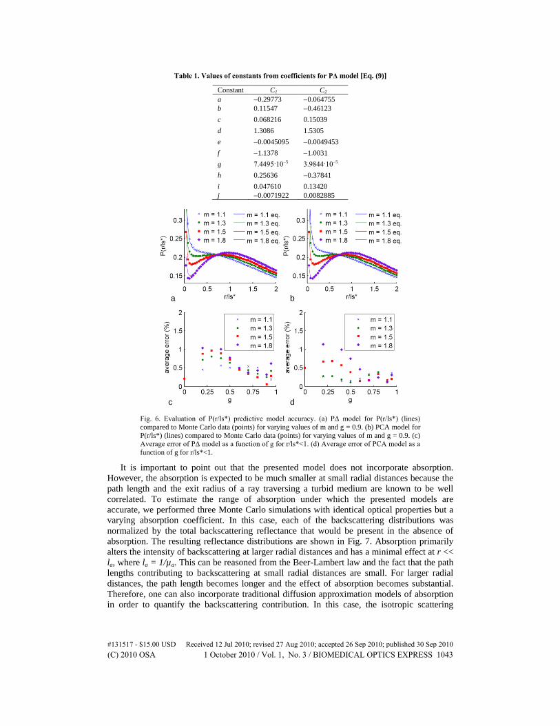
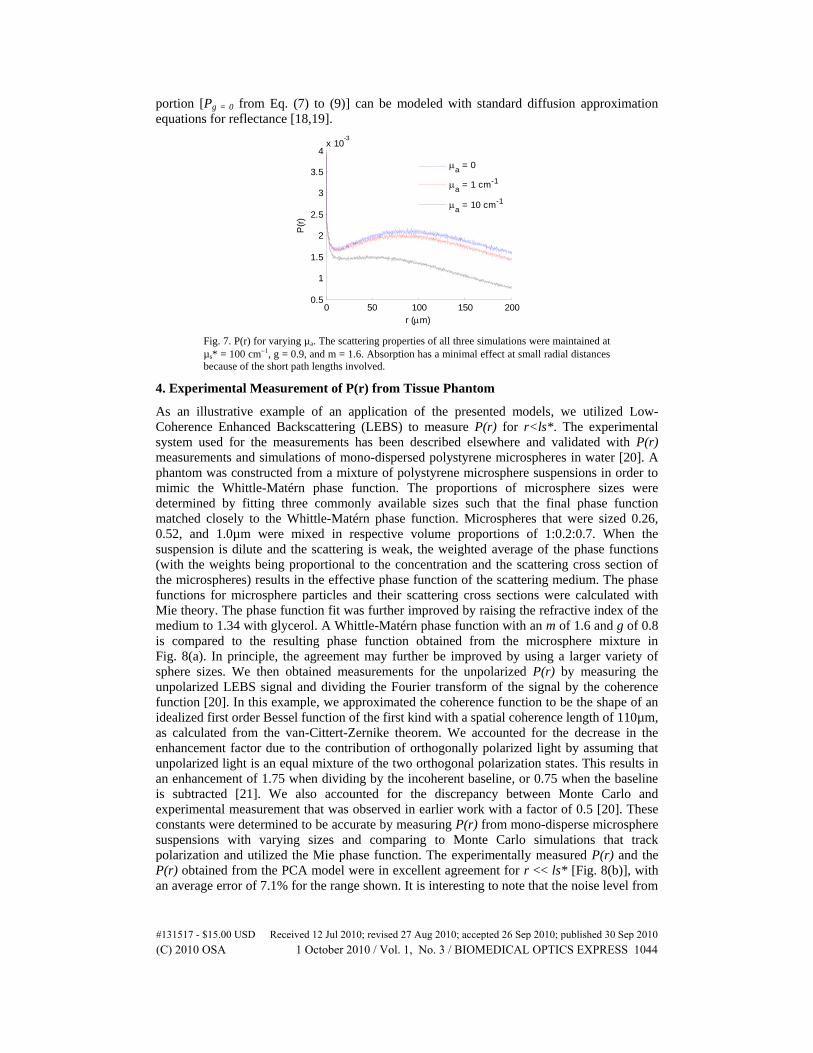
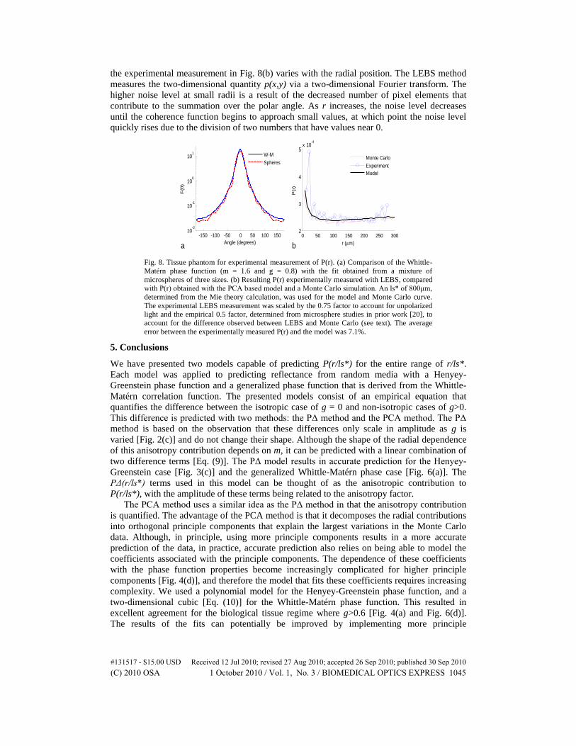
Related Documents