A practical guide to understanding Kaplan-Meier curves

Otolaryngology–Head and Neck Surgery (2010) 143, 331-336

INVITED ARTICLE

A practical guide to understanding Kaplan-Meier

curves

Jason T. Rich, MD, J. Gail Neely, MD, Randal C. Paniello, MD,Courtney C. J. Voelker, MD, DPhil, Brian Nussenbaum, MD, and

Sponsorships or competing interests that may be relevant to con-tent are disclosed at the end of this article.

ABSTRACT

In 1958, Edward L. Kaplan and Paul Meier collaborated to publisha seminal paper on how to deal with incomplete observations.Subsequently, the Kaplan-Meier curves and estimates of survivaldata have become a familiar way of dealing with differing survivaltimes (times-to-event), especially when not all the subjects con-tinue in the study. “Survival” times need not relate to actualsurvival with death being the event; the “event” may be any eventof interest. Kaplan-Meier analyses are also used in nonmedicaldisciplines.The purpose of this article is to explain how Kaplan-Meier curvesare generated and analyzed. Throughout this article, we will dis-cuss Kaplan-Meier estimates in the context of “survival” beforethe event of interest. Two small groups of hypothetical data areused as examples in order for the reader to clearly see how theprocess works. These examples also illustrate the crucially impor-tant point that comparative analysis depends upon the whole curveand not upon isolated points.

© 2010 American Academy of Otolaryngology–Head and NeckSurgery Foundation. All rights reserved.

In 1958, Edward L. Kaplan and Paul Meier collaboratedto publish a seminal paper on how to deal with incom-

plete observations.1 Subsequently, the Kaplan-Meier (K-M)curves and estimates of survival data have become a famil-iar way of dealing with differing survival times (times-to-event), especially when not all the subjects continue in thestudy. Examples of when times-to-events may be importantend-point variables include cancer survival times, tympa-nostomy tube duration, onset times of hypocalcemia follow-ing parathyroid resection, or duration of nasal congestionfollowing septoplasty. As illustrated by these examples,“survival” times need not relate to actual survival with deathbeing the event; the “event” may be any event of interest.K-M analyses are also used in nonmedical disciplines.

The purpose of this article is to explain how K-M curvesare generated and analyzed. Throughout this article, we will

Received April 17, 2010; accepted May 10, 2010.

0194-5998/$36.00 © 2010 American Academy of Otolaryngology–Head and Necdoi:10.1016/j.otohns.2010.05.007

discuss K-M estimates in the context of “survival” beforethe event of interest. Two small groups of hypothetical dataare used as examples in order for the reader to clearly seehow the process works. These examples also illustrate thecrucially important point that comparative analysis dependsupon the whole curve and not upon isolated points.

Important General Concepts

Time-to-event is a clinical course duration variable for eachsubject, having a beginning and an end anywhere along thetime line of the complete study. For example, it may beginwhen the subject is enrolled into a study or when treatmentbegins, and ends when the end-point (event of interest) isreached or the subject is censored from the study (more onthis later). This duration is known as serial time, describingthe clinical-course time, in contrast to calendar (also knownas secular) time. Calendar time refers to the way we usuallythink of time and the way clinical trials are designed (Fig 1).In most clinical trials, individual subjects may enter or beginthe study (zero time) and reach end-point at vastly differingpoints along the trial calendar (Fig 2).

In preparing K-M survival analysis, each subject is char-acterized by three variables: 1) their serial time, 2) theirstatus at the end of their serial time (event occurrence orcensored), and 3) the study group they are in. These com-ponents may be displayed in a table (Table 1). For the con-struction of survival time probabilities and curves, the serialtimes for individual subjects are arranged from the shortestto the longest, without regard to when they entered thestudy. By this maneuver, all subjects within the group beginthe analysis at the same point and all are surviving untilsomething happens to one of them. The two things that canhappen are: 1) a subject can have the event of interest or 2)they are censored.

Censoring means the total survival time for that subjectcannot be accurately determined. This can happen whensomething negative for the study occurs, such as the subjectdrops out, is lost to follow-up, or required data are not

k Surgery Foundation. All rights reserved.

332 Otolaryngology–Head and Neck Surgery, Vol 143, No 3, September 2010

available or, conversely, something good happens, such asthe study ends before the subject had the event of interestoccur, i.e., they survived at least until the end of the study,but there is no knowledge of what happened thereafter.Thus, censoring can occur within the study or terminally atthe end. Note in Figure 2, censoring has occurred within thestudy and terminally. This makes sense only if one remem-bers that it is the duration of known survival that is beingmeasured. If a subject survives to the end of the studywithout an event, his/her total survival is not known; it is notappropriate to consider his/her time interval as an indicatorof the survival time.2,3 For example, if subject #1 has anevent of interest at two years and subject #2 has been in thestudy for only one year before the study ends, it is notappropriate to say that subject #2 has a survival of one year.

Figure 1 This figure illustrates the component parts of a clin-ical trial. Each trial may differ; however, all require a start-upperiod, and end of accrual, and an end to the trial.

Figure 2 This figure illustrates subjects entering a trial andending at different times. S, M, and L indicate short, medium, andlong serial times. The solid circle represents an event occurrence

Subject #2 could have died 20 years later or 20 hours later.It helps to understand this further if we remember thatclinically, we may get information on our patients indefi-nitely; however, research is expensive, has a beginning andan end, and is formally closed when the study is complete(figuratively, the lights go off, the telephones are not an-swered, and files are stored, and everyone goes to anotherjob).

The serial time duration of known survival is terminatedby the event of interest; this is known as an interval in K-Manalysis and is graphed as a horizontal line (more on thislater). In other words, only event occurrences define knownsurvival time intervals. Censored subjects are indicated onthe K-M curve as tick marks; these do not terminate theinterval.

Preparation for K-M Analysis

Raw data are stored using actual calendar dates and times.During analysis, serial times may be automatically calcu-lated and these used in curve construction and analysis.

The first step in preparation for K-M analysis involvesthe construction of a table using an Excel spreadsheet orWord document table (Microsoft Corporation, Redmond,WA) containing the three key elements required for input.These are: 1) serial time, 2) status at serial time (1 � eventof interest; 0 � censored), and 3) study group (e.g., group 1or 2). The table is then sorted by ascending serial times,beginning with the shortest times for each group (Table 1).Notice that each group has one censored subject. In group 1,the subject made it to the end of the trial and was terminallycensored; in group 2, the subject was censored within aninterval within the study time line.

Once this initial table is constructed, K-M analysis, usinga statistical program such as SPSS (SPSS Inc., Chicago, IL),SigmaPlot (Systat Software, Inc., San Jose, CA), or OriginPro(Origin Lab Corp., Northampton, MA), is simple. Because

Table 1

Initial sorted table for Kaplan-Meier analysis

SubjectSerial time

(yrs)Status at serial time

(1 � event; 0 � censored)Group(1 or 2)

B 1 1 1E 2 1 1F 3 1 1A 4 1 1D 4.5 1 1C 5 0 1U 0.5 1 2Z 0.75 1 2W 1 1 2V 1.5 0 2X 2 1 2Y 3.5 1 2

any long duration times may dominate means, medians and

333Rich et al A practical guide to understanding Kaplan-Meier curves

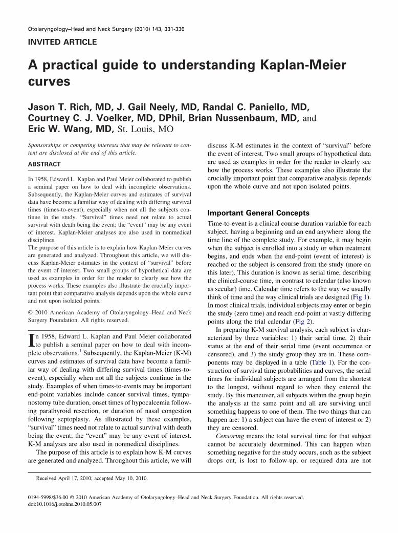
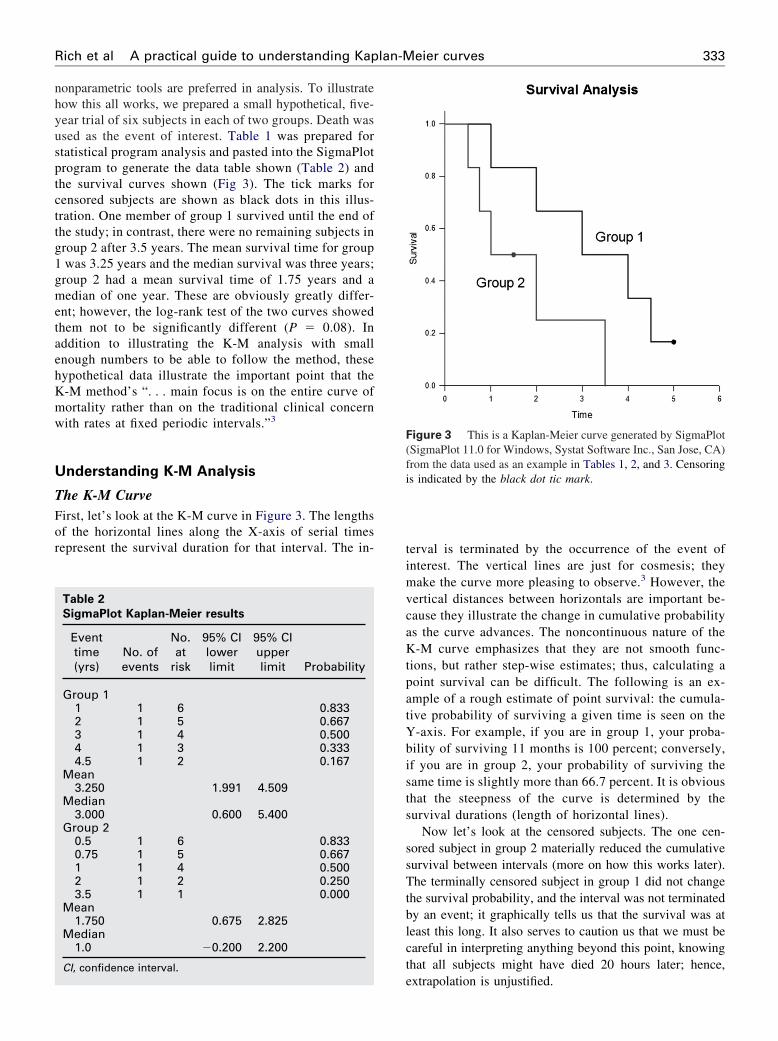
nonparametric tools are preferred in analysis. To illustratehow this all works, we prepared a small hypothetical, five-year trial of six subjects in each of two groups. Death wasused as the event of interest. Table 1 was prepared forstatistical program analysis and pasted into the SigmaPlotprogram to generate the data table shown (Table 2) andthe survival curves shown (Fig 3). The tick marks forcensored subjects are shown as black dots in this illus-tration. One member of group 1 survived until the end ofthe study; in contrast, there were no remaining subjects ingroup 2 after 3.5 years. The mean survival time for group1 was 3.25 years and the median survival was three years;group 2 had a mean survival time of 1.75 years and amedian of one year. These are obviously greatly differ-ent; however, the log-rank test of the two curves showedthem not to be significantly different (P � 0.08). Inaddition to illustrating the K-M analysis with smallenough numbers to be able to follow the method, thesehypothetical data illustrate the important point that theK-M method’s “. . . main focus is on the entire curve ofmortality rather than on the traditional clinical concernwith rates at fixed periodic intervals.”3

Understanding K-M Analysis

The K-M CurveFirst, let’s look at the K-M curve in Figure 3. The lengthsof the horizontal lines along the X-axis of serial timesrepresent the survival duration for that interval. The in-

Table 2

SigmaPlot Kaplan-Meier results

Eventtime(yrs)

No. ofevents

No.at

risk

95% CIlowerlimit

95% CIupperlimit Probability

Group 11 1 6 0.8332 1 5 0.6673 1 4 0.5004 1 3 0.3334.5 1 2 0.167

Mean3.250 1.991 4.509

Median3.000 0.600 5.400

Group 20.5 1 6 0.8330.75 1 5 0.6671 1 4 0.5002 1 2 0.2503.5 1 1 0.000

Mean1.750 0.675 2.825

Median1.0 �0.200 2.200

CI, confidence interval.

terval is terminated by the occurrence of the event ofinterest. The vertical lines are just for cosmesis; theymake the curve more pleasing to observe.3 However, thevertical distances between horizontals are important be-cause they illustrate the change in cumulative probabilityas the curve advances. The noncontinuous nature of theK-M curve emphasizes that they are not smooth func-tions, but rather step-wise estimates; thus, calculating apoint survival can be difficult. The following is an ex-ample of a rough estimate of point survival: the cumula-tive probability of surviving a given time is seen on theY-axis. For example, if you are in group 1, your proba-bility of surviving 11 months is 100 percent; conversely,if you are in group 2, your probability of surviving thesame time is slightly more than 66.7 percent. It is obviousthat the steepness of the curve is determined by thesurvival durations (length of horizontal lines).

Now let’s look at the censored subjects. The one cen-sored subject in group 2 materially reduced the cumulativesurvival between intervals (more on how this works later).The terminally censored subject in group 1 did not changethe survival probability, and the interval was not terminatedby an event; it graphically tells us that the survival was atleast this long. It also serves to caution us that we must becareful in interpreting anything beyond this point, knowingthat all subjects might have died 20 hours later; hence,

Figure 3 This is a Kaplan-Meier curve generated by SigmaPlot(SigmaPlot 11.0 for Windows, Systat Software Inc., San Jose, CA)from the data used as an example in Tables 1, 2, and 3. Censoringis indicated by the black dot tic mark.

extrapolation is unjustified.

334 Otolaryngology–Head and Neck Surgery, Vol 143, No 3, September 2010

Data and Calculations behind the CurveA more detailed look at what happens in the production ofthe K-M curve is seen in Table 3. When cross-referencingTable 3 with Figure 3, it becomes apparent that intervals(horizontal lines in the K-M curve) and the attendant prob-abilities are constructed only for events of interest and notfor censored subjects. Because an event ends one intervaland begins another interval, there should be more intervalsthan events; in other words, there is one event between twointervals. It is easier to see this connection by looking at theverticals or the ends of the intervals (or corners joininghorizontal with vertical). Thus, in group 1 and in group 2,there are five events (vertical connection between end ofone interval and beginning of the next) demarcating sixintervals (horizontals); note again that there is no verticalchange associated with the censored subjects. It is alsoobvious that the interval durations are variable; being ableto deal with varying interval durations is a particularstrength of the K-M method. The table helps explain theway the curves end. In group 1, the curve ends withoutcreating another interval below. The cumulative probabilityof surviving this long is determined by the last horizontal,sixth interval, and is 0.167. In group 2, the curve drops tozero after the fifth interval to cause the sixth interval hori-zontal to be on the X-axis.

Now let’s look at the probabilities of “survival.” The twodifferent probabilities can be a little confusing. There is acumulative probability and an interval probability. The cu-mulative probability defines the probability at the beginningand throughout the interval. This is graphed on the Y-axisof the curve. The interval survival rate (or probability)defines the probability of surviving past the interval, i.e.,still surviving after the interval and beginning the next. Thefirst intervals characteristically begin at zero time and endjust prior to the first event. For example, in group 1, intervalone begins at zero time with six subjects having a cumula-

Table 3

Full accounting of data

Subject

Serial time (yrs)(serial time of

event, � “eventtime”)

Interval(ending at

eventoccurrence)

Number “surviving” at riskin the interval (defines the

denominator for theinterval)

Event(definesend of

interval)

C(rem“suth

Group 1 0 1B 1 2 6 1E 2 3 5 1F 3 4 4 1A 4 5 3 1D 4.5 6 2 1C 5 0

Group 2 0 1U 0.5 2 6 1Z 0.75 3 5 1W 1 4 4 1V 1.5 0X 2 5 2 1Y 3.5 6 1 1

Calc, calculation.

tive survival rate of 6 of 6, or 1.0. At serial time 1 year, an

event occurred leaving five surviving the interval to go on tointerval two; thus, the probability of surviving up to year 1is 6 of 6, and the probability of surviving past 1 year is 5 of6 � 0.833. Cumulative probabilities for an interval arecalculated by multiplying the interval survival rates up tothat interval. For example, the chances of survival begin ininterval one as 6 of 6, then are 5 of 6 in interval two, and 4of 5 for interval three, giving a cumulative survival rate(probability) in interval three of 6/6 � 5/6 � 4/5 � 0.667.The next thing to note is that the Y-axis in the curve relatesonly to the cumulative probability of the interval but doesnot tell us how many subjects were in the numerator or thedenominator for each interval.

Censoring has an effect on the survival rates. Censoredobservations that coincide with an event are usually consid-ered to fall immediately after the event. Censoring removesthe subject from the denominator, i.e., individuals still atrisk. For example, in group 2, there were three survivinginterval four and available to be at risk in interval five.However, during interval four, one was censored; therefore,only two were left to be at risk in interval five, i.e., as seenin Table 2, the denominator went from four in interval fourto two in interval five.

Comparison of K-M Estimates

As tempting as it is to look at a series of time points, toproperly compare the two curves requires analysis tech-niques that consider the “. . . entire curve of mortality . . .”3

Comparing survival curves is of particular interest in clin-ical trials. While it is simple to visualize the differencebetween two survival curves, the difference must be quan-tified in order to assess statistical significance. Plottingconfidence intervals can be useful in visualizing the differ-ences. The mathematical computations for these analysesare beyond the scope of this article, but will be presented in

minl)

Number “surviving”after event (defines

the numerator)

Calc: interval“survival”rate after

event

Interval“survival”rate after

eventCalc: cumulative“survival” rate

Cumulative“survival”

rate

1.0005 5 of 6 0.833 1.000 * 0.833 0.8334 4 of 5 0.800 0.833 * 0.800 0.6673 3 of 4 0.750 0.667 * 0.750 0.5002 2 of 3 0.667 0.500 * 0.667 0.3331 1 of 2 0.500 0.333 * 0.500 0.167

1.0005 5 of 6 0.833 1.000 * 0.833 0.8334 4 of 5 0.800 0.833 * 0.800 0.6673 3 of 4 0.750 0.667 * 0.750 0.500

1 1 of 2 0.500 0.500 * 0.500 0.250 0 of 1 0 0.25 * 0 0

ensoredoved fro

rviving”e interva

000001

000100

their generalities.

335Rich et al A practical guide to understanding Kaplan-Meier curves

The log-rank test is the most common method. Thelog-rank test calculates the �2 for each event time for eachgroup and sums the results. The summed results for eachgroup are added to derive the ultimate �2 to compare the fullcurves of each group. The log-rank test for the data in ourexample was P � 0.80; thus, the two curves are not statis-tically significantly different. This is likely because suchsmall numbers in the sample do not have the power to ruleout a real difference and avoid a type-two error (falsenegative). For a thorough description of this process, thereader is referred to Douglas G. Altman’s text, PracticalStatistics for Medical Research.2

Another method of comparing K-M curves is using thehazard ratio, which gives a relative event rate in the groups.Again, the same cumulative process of calculating the �2 foreach event time and summing the results, giving the finalobserved and expected numbers for the full K-M curve asperformed in the log-rank test; thus, the hazard ratio refersto the results of the full curves.2 Statistical programs makethese calculations within seconds; however, it is helpful tounderstand what they are doing.

Different K-M Curves Used in Cancer

Literature

Some studies may use a combination of different types ofsurvival curves to express their data. The main differencebetween the curves is what is defined as the event or end-point. In overall survival curves, the event of interest isdeath from any cause. This provides a very broad, generalsense of the mortality of the groups. In disease-free survivalcurves, the event of interest is relapse of a disease ratherthan death. Because patients may have relapsed but not yetdied, disease-free survival curves are lower than overallsurvival curves. Progression-free survival uses progressionof a disease as an end-point (i.e., tumor growth or spread).This is useful in isolating and assessing the effects of aparticular treatment on a disease. Disease-specific survivalcurves (also known as cause-specific survival) utilize deathfrom the disease of interest as the end-point. This curve canbe misleading in that it will always be higher than overallsurvival, and disease-free survival curves because events arelimited only to death from a specific disease, i.e., patientsthat have disease relapse or die from nonrelated causes arenot included as events. In addition, death caused by disease-related factors (i.e., treatments) may not be included indisease-specific survival curves.

Considerations and Pitfalls of K-M Curves

When analyzing a K-M survival curve, one must first iden-tify what is the event of interest and the units of measure-ment along the axes. Next, the shape of the curve is impor-tant to evaluate. Curves that have many small steps usuallyhave a higher number of participating subjects, whereascurves with large steps usually have a limited number of

The amount of censored subjects and the distribution ofcensored subjects are also important. If the number of cen-sored subjects is large, one must question how the study wascarried out or if the treatment was ineffective, resulting insubjects leaving the study to pursue different therapies. Acurve that does not demonstrate censored patients should beinterpreted with caution.

As mentioned above, �2 from the log-rank test willsuggest whether two curves are statistically different. TheCox proportional hazards will show the increased rate ofhaving an event in one curve versus the other.

Survival at different time points can also be obtained andcompared between curves. Studies will often include two-or five-year survival percentages for the survival curveswithin the text. If both curves pass through the 50 percentilemark, the median survivals for each curve can be quicklycompared. This is done by drawing a vertical line fromwhere the curve crosses the 50 percent down to the timeaxis.

Most clinical trials have a minimum follow-up time, atwhich point the status of each patient is known. The survivalrate at this point becomes the most accurate reflection of thesurvival rate of the group. Survivor function at the far rightof a K-M survival curve should be interpreted cautiouslysince there are fewer patients remaining in the study groupand the survival estimates are not as accurate.

For example, in a study looking at the survival of patientsreceiving treatment for stage I lung cancer, the medianfollow-up was 40 months.4 However, one of the 302 pa-tients had a follow-up at 10 years, and so a survival rate of92 percent (95% confidence interval [CI] 88-95%) at 10years was presented based on this one patient. Ninety-twopercent at 10 years appears to be a very good estimatedsurvival rate. However, with such a small subset of patientsat this time point, the K-M estimates can be misleading andshould be interpreted with caution. Carter and Huang5

pointed out that if this remaining patient had an event thefollowing month, the survival probability would dramati-cally drop to zero percent using the K-M calculations, withthe 95% CI zero to zero percent. Thus, the estimations ofsurvival from K-M analyses are most accurate at the timepoint when most patients are still present in the study. In thisexample, the median follow-up of the study was 40 months,and so the quoted survival rate of 92 percent (95% CI88%-95%) is a better representation of the four- or five-yearsurvival rate than the 10-year rate.5 This type of error can beavoided if authors include patients at risk (remaining sub-jects in the study) for each interval.

It should also be remembered that after the first patient iscensored, the survival curve becomes an estimate, since wedo not know if censored patients would have experienced anevent at some point later in their life. Thus, the morepatients that are censored in a study (especially early in thestudy), the less reliable is the survival curve. Likewise, it ishelpful to know why patients were censored. If many pa-

336 Otolaryngology–Head and Neck Surgery, Vol 143, No 3, September 2010

how the study was carried out or how the type of treatmentaffected the patients. This stresses the importance of show-ing censored patients as tick marks in survival curves.

Conclusion

We have described the basics of K-M survival curves byusing two very small comparison groups as examples so thatthe details of construction and analysis could be easily seen.Despite what appeared to be a great difference between thetwo very small groups, the log-rank test showed that the twocurves were not significantly different (P � 0.08). Thesehypothetical data illustrate a crucially important point: theKaplan-Meier method’s “. . . main focus is on the entirecurve of mortality rather than on the traditional clinicalconcern with rates at fixed periodic intervals.”3 Looking atthe ends of the curves or points within them may easily missthe real message.

Acknowledgment

The authors wish to acknowledge the support of Kathryn Trinkaus, PhD, ofthe Biostatistics Core, Siteman Comprehensive Cancer Center.

Author Information

From the Department of Otolaryngology–Head and Neck Surgery, Wash-

Corresponding author: J. Gail Neely, MD, Department of Otolaryngology–Head and Neck Surgery, Washington University School of Medicine, 660S. Euclid Avenue, Box 8115, St. Louis, MO 63110.

E-mail address: [email protected].

Author Contributions

Jason T. Rich, major author; J. Gail Neely, major author and editor;Randal C. Paniello, contributing author and reader; Courtney C. J.Voelker, contributing author and reader; Brian Nussenbaum, contributingauthor and reader; Eric W. Wang, contributing author and reader.

Disclosures

Competing interests: None.

Sponsorships: This work was supported by National Cancer InstituteCancer Center Support Grant P30 CA091842.

References

1. Kaplan EL, Meier P. Nonparametric estimation from incomplete obser-vations. J Am Stat Assoc 1958;53:457–81.

2. Altman DG. Practical Statistics for Medical Research. New York:Chapman & Hall/CRC; 1991. p. 365–96.

3. Feinstein AR. Clinical Epidemiology: The Architecture of ClinicalResearch. Philadelphia: W. B. Saunders Co.; 1985. p. 226–7, 335,343–6.

4. Henschke CI, Yankelevitz DF, Libby DM, et al. Survival of patientswith stage I lung cancer detected on CT screening. N Engl J Med2006;355:1763–71.

5. Carter RE, Huang P. Cautionary note regarding the use of CIs obtained