A power-enhanced algorithm for spatial anomaly detection in binary labelled point data using the spatial scan statistic

promoting access to White Rose research papers

White Rose Research Online [email protected]

Universities of Leeds, Sheffield and York http://eprints.whiterose.ac.uk/

This is an author produced version of a paper to be published in Lecture Notes in Artificial Intelligence.

White Rose Research Online URL for this paper: http://eprints.whiterose.ac.uk/11053/

Conference paper Read, S., Bath, P.A., Willett, P. and Maheswaran, R. (2010) A Power-Enhanced Algorithm for Spatial Anomaly Detection in Binary Labelled Point Data Using the Spatial Scan Statistic [postprint]. In: 14th International Conference on Knowledge-Based and Intelligent Information & Engineering Systems, Sept 8th-10th, Cardiff UK. Lecture Notes in Artificial Intelligence, II (6277). Springer Verlag , Berlin. (In Press)

http://eprints.whiterose.ac.uk/11053/

A Power-Enhanced Algorithm for SpatialAnomaly Detection in Binary Labelled Point

Data Using the Spatial Scan Statistic

Simon Read1, Peter Bath1 Peter Willett1, and Ravi Maheswaran2

1 Department of Information Studies, University of Sheffield, Sheffield S1 4DP, [email protected]

2 ScHARR, University of Sheffield, Sheffield S1 4DA, UK

Abstract. This paper presents a novel modification to an existing al-gorithm for spatial anomaly detection in binary labeled point data sets,using the Bernoulli version of the Spatial Scan Statistic. We identify a po-tential ambiguity in p-values produced by Monte Carlo testing, which (bythe selection of the most conservative p-value) can lead to sub-optimalpower. When such ambiguity occurs, the modification uses a very in-expensive secondary test to suggest a less conservative p-value. Usingbenchmark tests, we show that this appears to restore power to the ex-pected level, whilst having similarly retest variance to the original. Themodification also appears to produce a small but significant improvementin overall detection performance when multiple anomalies are present.

1 Introduction

The detection of spatial anomalies (a.k.a. ‘spatial cluster detection’) in binarylabeled point data has important applications in analyzing the geographic dis-tribution of health events (e.g. [1]) and other fields such as forestry (e.g. [2]).Since 1997, the freely available SaTScanTMsoftware package (www.satscan.org)has provided a means of detecting such anomalies using the Spatial Scan Statis-tic [3] and has been used in well over a hundred published scholarly studies [4].Section 2 gives more details of the research context.

Combined with a moving scan window procedure, the statistic identifies thelocation, size and statistical significance (p-value) of potential anomalies withina given study region. Due to the nature of the Spatial Scan Statistic as it iscurrently applied to binary labeled point data (see primer in Section 3), it issometimes not possible to establish an exact p-value for the most likely poten-tial anomaly. This ambiguity can occur in various places on the unit interval,including the most useful part of the range, 0 ≤ p-value ≤ 0.1. This issue isexplained in Section 4. When ambiguity occurs, SaTScanTMselects the mostconservative p-value, resulting in a sometimes lower-than-expected false positiverate (FPR), and a corresponding reduction in true positive rate (TPR, a.k.a.statistical power or sensitivity).

The principal contribution of this paper is to describe a means by which,when p-value ambiguity occurs, otherwise redundant information can be used

Post-print to appear in LNAI, http://www.springer.com/series/1244

(Proceedings of KES2010, Sept 8th-10th, Cardiff UK)

to meaningfully (and consistently) suggest a less conservative p-value. This isdescribed in Section 5. Using benchmark tests (Section 6) we show this producesa false positive rate very close to the nominal significance level, and correspond-ingly increases the power in the circumstances outlined above. The proposedalgorithm also delivers a p-value consistency (i.e. mean retest variance) compa-rable to SaTScanTM

The secondary contribution is that, when applied to data sets where severalanomalies are present, the modification appears to produce a small improvementin the ratio of true and false positive rates, as measured using area under curve(AUC) as applied to ROC curves. We use a ‘within datasets’ Monte Carlo methodto show this improvement to be statistically significant, as described in Section6. A discussion of the results, and future research directions, is given in Section7.

2 Research Context

Spatial anomaly detection has three broad categories: global (identifying if anyanomaly is present in the study region, but not specifying a location); localised(as global, but specifying location) and focused (testing for the presence of ananomaly at a location specified a priori). The Spatial Scan Statistic [3] is awidely use method of localised anomaly detection. Localised is the most flexible,as it can perform the function of the other two, albeit possibly with sub-optimumpower. Following on from [3] many frequentist versions of the statistic have beendeveloped and compared, (see list in [4]) as well a Bayesian version [5]. Mostlythese are for use with areal data, e.g. disease counts in postal districts. TheBernoulli version (hereafter SSSB), is for use with binary labeled point data.Despite being introduced in [3] and used in various studies since (e.g. [1], [2]),there has been little research into the benchmark performance of the SSSB .Recently [6] used the SSSB when considering a alternative circular scan windowselection method (scan windows, termed here Zj , are defined in Section 3), and[7] have developed a risk-adjusted SSSB variant. Although the latter is of someinterest, it appears to have lower-than-expected FPR and TPR, so in this paperwe only consider the original SSSB . It is also worth noting that many studieshave been published into the effect of using different shaped scan windows, ofwhich a useful summary is given in [8]. The results of this study should beapplicable to all types of scan window, provided they can be applied to pointdata.

3 Primer: Spatial Scan Statistic (Bernoulli version)

The Spatial Scan Statistic has several versions. The Bernoulli (hereafter SSSB)is suitable to binary labeled point data. For the benefit of readers unfamiliarwith the Spatial Scan Statistic, this section formally defines3 the SSSB , its ac-

3 Regarding notation: italic lower-case = scalar; italic upper-case = set (or multiset),bold upper-case = set (or multiset) of sets (or multisets).

2



companying data structures and method of application 4. For a derivation of thestatistic see [3].

Consider a spatial region R , with r any point location therein. Consider adata set P = {p1,p2...pN} where each pi is associated a single point locationloci ∈ R, and a binary label si. Let P0 = {pi : si = 0} and P1 = {pi : si = 1},such that P0 ∪ P1 = P and P0 ∩ P1 = �. Let N and the position of each loci betaken as given, but assume each si value to be the outcome of an independentBernoulli trial with probability p(si = 1) = ρ(r), where ρ(r) is some arbitraryvalue (on the unit interval) associated with point r. Let H0 represent the (null)hypothesis that ρ(r) is constant for all r ∈ R. That is, the distribution of theelements of P1 amongst P is uniformly random. Let HA represent the (alternate)hypothesis that a spatial anomaly is present, i.e. there is a subset of R whereρ(r) is higher (or lower) than the rest of R. Put formally, HA ⇔ (∃A ⊂ R, hence∃B = R − A) such that ρ(a ∈ A) = βρ(b ∈ B), where β is a constant5 6= 1. Inthis study we only consider β > 1, but the results will apply equally to β < 1.This Bernoulli model is useful for representing point occurrences in many real-world applications, as it controls for a inhomogeneous underlying distribution ofevents.

In real data sets, A (if it exists) can only be estimated by guessing whichloci lie inside or outside it. Let us call any particular estimate Z. Furthermore,let us assume we have some predefined scheme (typically a moving scan windowof variable size) for generating a set of estimates, Z = {Z1, Z2, Z3 . . .}, whereeach Zj ⊂ P . The purpose of the SSSB is to determine which Zj (let us call thisZprime) is most likely to represent6 A, if indeed A exists. We then associate ap-value with Zprime, which represents the probability that H0 is true (in whichcase Zprime is a random artefact). To use the SSSB , we split all Zj such thatZj0 = {pi : pi ∈ Zj and si = 0} and Zj1 = {pi : pi ∈ Zj and si = 1}. Foreach Zj the SSSB takes four integer inputs (N = |P |, C = |P1|, n = |Zj | andc = |Zj1|) and produces one quasi-continuous output, the log likelihood ratio orLLR. The formula is given in three parts: Equation 17 gives the likelihood ofHA if Zj represents A; Equation 2 gives the likelihood of H0, identical of allchoices of Zj . Equation 38 brings the two values together to produce the LLR.Testing all Zj ∈ Z using the SSSB gives a multiset L of LLR values, whereL = {llr1, llr2, llr3, . . .}. Zprime is then Zj for which llrj ≥ llrk∀k 6= j (let uscall this llrprime). In the case of multiple maximum LLR values, an arbitrarychoice for Zprime is made.

4 SSSB can also be applied to spatio-temporal data, not discussed here.5 Note an assumption of uniform probability inside and outside the anomaly is required

by the Spatial Scan Statistic.6 By represent, we mean pi ∈ Zprime ⇒ loci ∈ A and pi /∈ Zprime ⇒ loci /∈ A7 Note I represents the indicator function.8 Note any log base can be used, provided it is consistent throughout the study.

3



LA(Zj) = (n

c)c(1− n

c)(n−c)(

C − cN − n

)C−c(1− C − cN − n

)(N−n−C+c)I(c

n>

C − cN − n

)

(1)

L0 = (C

N)C(

N − CN

)(N−C) (2)

llrj = logLA(Zj)

L0(3)

The p-value of Zprime is obtained by randomisation testing. For step m (ofM Monte Carlo steps) the si values of all points are pooled and randomlyre-allocated. The above procedure is repeated, generating a new multiset Lm

of LLR values. For each Lm the maximum LLR (llrprime−m) is recorded andstored in multiset D where D = {llrprime−1, llrprime−2, . . . llrprime−M}. If H0

is true, the ‘real’ value llrprime should fall comfortably within the distributionof llrprime−m values9. To calculate the p-value10 of Zprime using the establishedSaTScanTMprocedure, we count the number of llrprime−m ≥ llrprime (let’s callthis v) and set the p-value to (v + 1)/(M + 1). This Monte Carlo procedure iscompatible with most versions of the Spatial Scan Statistic, but it sometimescreates a particular problem when used with the SSSB , discussed in Section 4.

4 Problem Identification

All versions of the Spatial Scan Statistic share a common characteristic of beingthe individually most powerful test for a localised anomaly [3]. This means ifa particular HA is true (see Section 3), then for a given Z and a given FPR(i.e. probability of Type I error), no test can have a greater chance of correctlyrejecting H0. Of course, this assumes one is in control of the FPR. In benchmarktests conducted by the author using some other versions of the Spatial ScanStatistic (not presented here), the FPR the Spatial Scan Statistic is generallyvery close to the nominal significance level (hereafter α). However, for the SSSB

the FPR is sometimes markedly lower than α, which correspondingly reducesthe TPR (a.k.a power). An explanation is given below.

As described in Section 3, the SSSB has four integer input parameters (N , C,n, c), and one quasi-continuous output parameter, the LLR. Within any givendata set, N and C are constant, leaving only two free integer parameters. Thusmany scan windows (Zj ∈ Z) share duplicate LLR values, which also producesduplicate llrprime−m values in D. The problem arises when multiple values inD match the ‘real’ llrprime, as one then has a range of equally valid p-valuesto choose from. SaTScanTMdefers to the most conservative p-value, by setting vto the count of all llrprime−m ≥ llrprime. This is not in any way incorrect, butit does lead unavoidably to the drop in FPR and TPR mentioned above. Onecan instead set v to the count of all llrprime−m > llrprime; this leads to higher

9 Under H0 ρ(r) is uniform, so randomising si has little affect on llrprime10 Other Zj with high llrj may also be of interest, but this is not our concern here.

4



TPR but also a FPR significantly higher than α, which may not be acceptable tousers. Of course this is only a problem when these multiple p-values straddle α.Unfortunately, in both sets of benchmark tests presented in this paper, a rangeof equally likely p-values frequently occurs that includes the popular α valuessuch as 0.05. Increasing the number of Monte Carlo repetitions does not help,as the number of duplicates increases also.

If we are only concerned about the veracity of outcomes when averaged overmany datasets, we could simply select a uniformly randomly p-value somewherebetween the highest and lowest p-value (inclusive) in the ambiguous range. How-ever, such a speculative p-value is clearly unacceptable in a real-world testingsituation. The user could look for an alternative source of information about thedata points instead, but an internal solution would clearly be preferable. As-suming the point locations and status are all we have, the only way of obtainingadditional information is perform a different type of anomaly test, ideally oneunlikely to produce duplicate values. Then we can then associate a secondaryvalue with each LLR, enabling us to rank the llrprime value amongst many iden-tical llrprime−m values. The problem then chiefly becomes one of computationtime, as one must multiply the cost of the secondary test by M+1. The followingsection outlines a potential, time-efficient, solution.

5 Proposed Solution

As a secondary anomaly test (to help resolve p-value ambiguity) one can makeuse of the values in L and Lm (the sets of all LLR values obtained from boththe ‘real’ data and each Monte Carlo step). These are a reservoir of information,most of which is discarded. Most of these LLR values are close to zero, as theycorrespond to Zj in which |Zj0| and |Zj1| are wholly compatible with H0. How-ever, when an anomaly is present, many Zj (aside from Zprime) may partiallyoverlap or wholly include the anomaly A. Thus we may have many unusuallyhigh llrj values, even if only one anomaly is present. Therefore the mean llrjvalue (hereafter llr) should generally be higher when an anomaly is present11.

Of course, we would not ordinarily use llr as a test statistic when manywell established global anomaly tests exist. However, llr is very inexpensive tocalculate, making it attractive as a secondary test (for reasons outlined in Section4). Using the original procedure, we must calculate every llrj to find Zprime. So,these values must all be present within the processor at some point, and we canuse cache memory (perhaps even a spare register) to hold the running total.The cost of each addition, compared to the exponential/logarithmic operationsrequire to find the LLR, is minuscule. An algorithm to implement this, shownalongside the original algorithm, is given below. The line marked * is the stepthat accounts for the majority of the total computation time. The creation ofD′ is provided here only for illustrative purposes; if the elements of D are storedin a suitably ordered way, v can be calculated directly from D.

11 llr is therefore a ‘global’ anomaly detection statistic, as defined in Section 2.

5



Original Algorithm Proposed Algorithm

Load P0 and P1 from file Load P0 and P1 from fileGenerate Z and L Generate Z and L, note running total of llrjllrprime = max(L) llrprime = max(L)Note Zprime Note Zprime

Create empty set D llr =∑llrj/|L|

For m = 1 to M { Create empty set DShuffle all si values For m = 1 to M {* Generate Lm Shuffle all si valuesllrprime−m = max(Lm) * Generate Lm, note running total of llrmj

Insert llrprime−m into D llrprime−m = max(Lm)

} llrm =∑llrmj/|L|

D′(⊆ D) = {llrprime−m : Insert pairing { llrprime−m, llrm } into Dllrprime−m ≥ llrprime} }

v = |D′| D′(⊆ D) = { {llrprime−m, llrm} :p-value = (v + 1)/(M + 1) ( llrprime−m > llrprime ) or

Report Zprime and p-value ( llrprime−m = llrprime and llrm ≥ llr ) }v = |D′|p-value = (v + 1)/(M + 1)Report Zprime and p-value

6 Benchmark Results

The proposed algorithm shown above was coded in C++ and compared to theoriginal SaTScanTMsoftware using two batches of synthetic benchmark ‘case/control’ data. This section briefly describes the technical implementation, andpresents the results.

So that a direct comparison could be made, the generation of Z (and L) wasperformed using the same concentric circular method used by SaTScanTM. Thisinvolves generating a set of concentric circles centred on each loci, selecting onlythose circles with radii just sufficient to include loci′ (i 6= i′, and pi′ ∈ P1). Foreach circle, a scan window (Zj) is created containing all members of P whoselocation loci lies within this circle. A graphic example is given in [6]. Two batchesof synthetic data sets (BCSR and BTRENT ) were generated using a separateprogram. Both contain 6000 data sets: 3000 representing H0; 3000 representinga selected HA. Each data set contains the loci (two integer co-ordinates on a500×500 grid) of 300 points: 200 ‘controls’ (si = 0) and 100 ‘cases’ (si = 1).Regarding the control loci: for BCSR these were generated under complete spatialrandomness; for BTRENT they were generated using a Poisson process, witha p.d.f. in proportion to the 2001 population density of the Trent region ofthe UK, mounted onto the same 500×500 grid (full details given in [6]). Thisoffers comparison between homogeneous and inhomogeneous background pointdensity. Regarding the case loci: under H0 these follow the same distribution asthe control loci. For BCSR under HA, we chose to insert into each data set three

6



randomly located, isotropic, Gaussian shaped anomalies, each with a maximumrelative risk12 (hereafter MRR) of 15. For a fully illustrated description, see [6].To give comparison with a tougher test, for BTRENT (under HA), we insertedonly one such randomly placed Gaussian anomaly, also with MRR of 15.

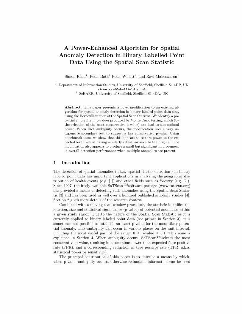
To assess performance, we obtained the p-value of both Zprime values (onegenerated by SaTScanTMand one by the proposed algorithm) for all data sets,using (M =)999 Monte Carlo steps. For each value of α in the range {0.001,0.002, . . . , 1} the count of p-values ≤ α was recorded for BCSR and BTRENT ,split into counts for H0 and HA. Dividing the H0 count by 3000 gives us theFPR (false positive rate, a.k.a. 1-specificity), and similarly for HA we have TPR(true positive rate, a.k.a. power or sensitivity). These are shown in Figure 1. Itcan be seen the FPR of the proposed algorithm is closer to parity across mostα values. As expected, the TPR of the proposed algorithm is also higher thanthat of SaTScanTMwhen the FPR of the latter dips below parity (due to p-valueambiguity in those ranges of α).

Although the proposed algorithm appears to rectify the overall drop in FRPand TPR, as mentioned in Section 4 we could have achieved this by simplyrandomising the p-value for each data set within its ambiguity range. Usersneed assurance the p-value suggested by a modified test is consistent, at leastsimilarly consistent to SaTScanTM. Table 1 shows the mean retest variance forboth tests, plus the randomised version just described. Here we selected 50 datasets at random from each of the 3000 H0 and HA data sets used for BCSR

and BTRENT . We then retested each data set 50 times, calculating the p-valuevariance. We then took the mean of this variance across the 50 data sets in eachbatch, shown in Table 1. The results show clearly the p-value consistency of theproposed algorithm is very close to that of SaTScanTM, and considerably betterthan the randomised version.

Data sets source — SaTScanTM— Proposed algorithm — Randomised algorithm

BCSR : H0 0.160 0.177 1.486

BCSR : HA 0.042 0.043 0.199

BTRENT : H0 0.140 0.159 1.291

BTRENT : HA 0.065 0.080 0.721

Table 1. Table showing mean retest variance (×10−3) of the different algorithms

Although the rectification of the FPR (and corresponding increase in TPR) isour main aim, it is also useful to test if the proposed algorithm has any noticeableeffect on overall detection performance (i.e. the ratio of TPR to FPR). Plottingthe pairings of FPR and TPR for each α value gives us the standard ROC(Receiver Operator Characteristic) curve for both SaTScanTMand the proposed

12 This is the amount of the relative increase in the probability of a case locationoccurring at the very centre of the anomaly, with the increase smoothly decreasing(following a Gaussian curve) as distance from the anomaly centre increases.

7



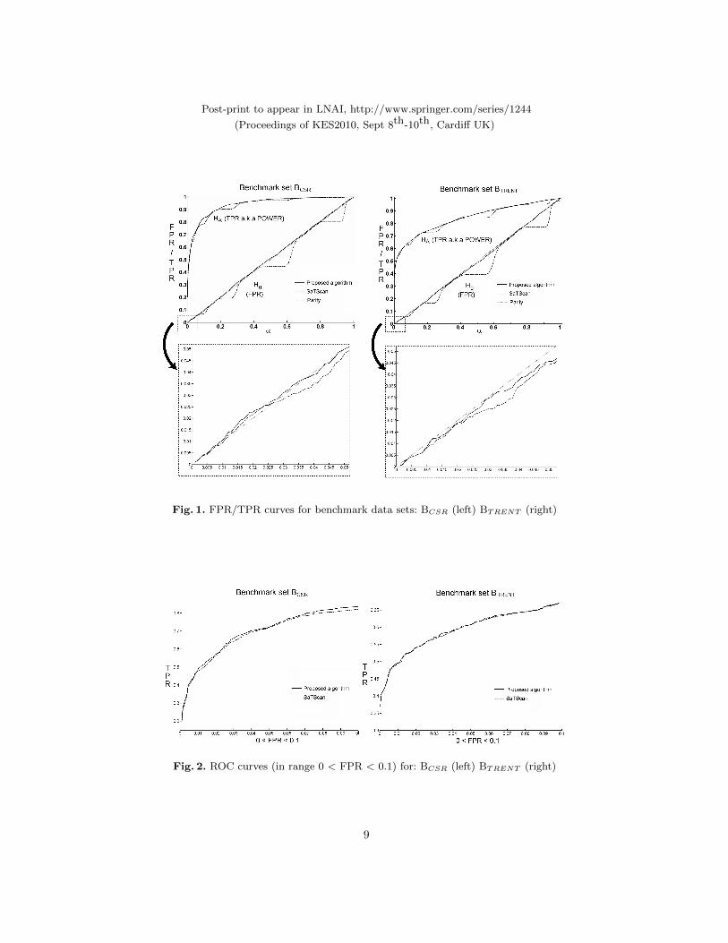
algorithm, as applied to BCSR and BTRENT . It has been proved [9] the areaunder a ROC curve (hereafter AUC) is equal to the probability that the test,when presented with one H0 and one HA data set, will correctly distinguishwhich is which. However, AUC is calculated using 0 <FPR≤ 1, and high FPRvalues (say above 0.1) are of little interest in most applications. We thereforechoose to calculate only the area under the curves in the range 0 <FPR≤ 0.1.Let’s call this AUC0.1.

Figure 2 shows both ROC curves in the range 0 <FPR≤ 0.1. It can be seenthe overall performance is very similar, especially for BTRENT (shown right).However, for BCSR (shown left) the ROC curve for the proposed algorithmshows slight improvement. For BCSR, the increase in AUC0.1 for the proposedalgorithm (over and above the AUC0.1 of SaTScanTM) is 1.44%, where as forBTRENT it is slightly negative at -0.62%. We used a ‘within data sets’ MonteCarlo procedure, developed by the author13, to establish a significance of<0.0001for the figure of 1.44% and 0.7929 for the figure of -0.62%. This indicates the con-fidence with which we may reject a null hypothesis that the increase in AUC0.1

(or decrease in the case of the -0.62% figure) is due solely to random variations intest performance. The significance levels suggest we can be confident that someperformance improvement occured in the BCSR data sets, whereas no significantdifference in performance occured in BTRENT data sets. The reason for this islikely to be the multiple anomalies present in the BCSR sets, an issue which isdiscussed further in Section 7.

7 Conclusion

In this paper we have identified a potential ambiguity in p-values produced bythe Bernoulli version of the Spatial Scan Statistic (SSSB), when used withinthe Monte Carlo algorithm with which it is normally associated. We proposedand tested a modified Monte Carlo algorithm which uses a very inexpensivesecondary test to produce a more precise p-value, with a retest consistency simi-lar to the p-value produced by the SaTScanTMsoftware. The proposed algorithmappears to restore false positive rate (FPR) to approximate parity with the nom-inal significance level of the test, and correspondingly increases the true positiverate (TPR), a.k.a. power. Two batches of 6000 data sets were used for bench-mark testing: one with three anomalies set against a homogeneous backgroundpoint density; one with a single anomaly set against a inhomogeneous back-ground point density. A similar rectification of FPR and TPR rates was seenacross both, and in the former a small (but statistically significant) increasein overall detection performance was also observed, as measured by area underROC curve in the critical area 0 <FPR< 0.1. The Spatial Scan Statistic has the

13 This involves randomly selecting 50% of data sets and swapping the p-values of thetwo tests, then recalculating the ratio of AUC0.1 for both tests. This swapping ispermissible under a null hypothesis that the underlying performance of the two testsis idenitcal. Repeating this (say 10,000 times) produces a distribution for the ratioof the two AUC0.1 values, against which the ‘real’ ratio can be measured.

8



Fig. 1. FPR/TPR curves for benchmark data sets: BCSR (left) BTRENT (right)

Fig. 2. ROC curves (in range 0 < FPR < 0.1) for: BCSR (left) BTRENT (right)

9



proven quality of being the individually most powerful test for localised anomalydetection [3], so this the latter claim may seem surprising. It is probably becauseof the definition of this characteristic is based on the test’s use of an alternatehypothesis containing only a single anomaly; the batch that witnessed the im-provement contains data sets with three anomalies. Due to its global nature, oursecondary test statistic (i.e. the mean LLR) may be sensitive to the presence ofmultiple anomalies in a way that the Spatial Scan Statistic (i.e. the maximumLLR) is not. This raises the question, even when there is no p-value ambiguityin the Spatial Scan Statistic, whether it might be useful to take the mean LLRinto account in some way.

We hope these results are of interest to the research community, and mayin future investigate the properties of other non-maximum LLR values with aview to gaining improvements in anomaly detection. It is expected any suchimprovements will apply equally to spatio-temporal point data, and this may bethe subject of future benchmark testing.

Acknowledgments

We wish to thank the Medical Research Council for funding Simon Read, theprincipal researcher, programmer and author. We also thank Professor StephenWalters of ScHARR, for his thoughts on the statistical comparison of ROCcurves.

References

1. Viel, J. F., Floret, N. and Mauny, F. (2005) Spatial and space-time scan statistics todetect low rate clusters of sex ratio, Environmental and Ecological Statistics, Volume12, Issue 3, pp 289-299.

2. Riitters, K. H. and Coulston J. W. (2005). Hot Spots of Perforated Forest in theEastern United States, Environmental Management, Volume 35, Issue 4, pp 483-492.

3. Kulldorff, M. (1997) A Spatial Scan Statistic, Communications in Statistics - Theoryand Methods, Volume 26, Issue 6, pp 1481-1496.

4. Kulldorff, M. (2009) SaTScanTMUsers Guide, available online:http://www.satscan.org/techdoc.html.

5. Neill, D. B., Moore, A. W. and Cooper, G. F. (2006) A Bayesian spatial scan statisticin Weiss, Y. (ed.) Advances in Neural Information Processing Systems, MIT Press,Cambridge, MA.

6. Read, S., Bath, P. A., Willett, P. and Maheswaran, R. (2009) A Spatial Accu-racy Assessment of an Alternative Circular Scan Method for Kulldorffs Spatial ScanStatistic in Fairbairn, D. (ed.) Proceedings of GISRUK09, Durham University, UK.

7. Taseli, A. and Benneyan, J. C. (2009) Risk Adjusted Bernoulli Spatial Scan Statis-tics, in Proceedings of the Industrial Engineering Research Conference (IERC) 2009,Institute of Industrial Engineers, Norcross, GA.

8. Tango, T. and Takahashi, K. (2005) A Flexibly Shaped Spatial Scan Statistic forDetecting Clusters, International Journal of Health Geographics, Volume 4, Issue 1.

9. J. A. Hanley and B. J. McNeil. (1982) The meaning and use of the area under areceiver operating characteristic curve, Radiology, Volume 143, Issue 1, pp 29-36.

10

A power-enhanced algorithm for spatial anomaly detection in binary labelled point data using the spatial scan statistic

Documents