A Post-Processor for Hydrologic Ensemble Forecast Products John Schaake, 1 Robert Hartman, 2 James Brown, 1 D.J. Seo 1 , and Satish Regonda 1 1. NOAA/NWS Office of Hydrologic Development 2. NOAA/NWS California-Nevada River Forecast Center Presentation to DOH Workshop July 16, 2008 Silver Spring

Welcome message from author
This document is posted to help you gain knowledge. Please leave a comment to let me know what you think about it! Share it to your friends and learn new things together.
Transcript
A Post-Processor for Hydrologic Ensemble Forecast Products
John Schaake,1 Robert Hartman,2 James Brown,1D.J. Seo1, and Satish Regonda1
1. NOAA/NWS Office of Hydrologic Development2. NOAA/NWS California-Nevada River Forecast Center
Presentation toDOH Workshop
July 16, 2008Silver Spring
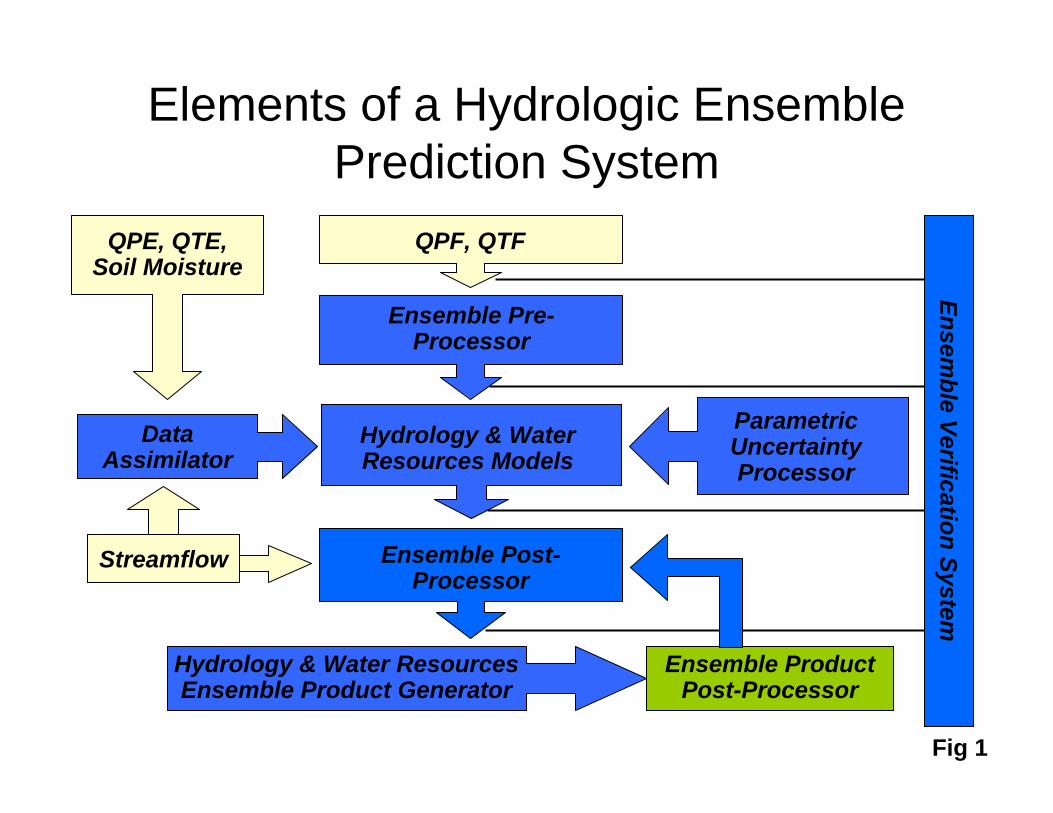
Elements of a Hydrologic Ensemble Prediction System
Ensemble Pre-Processor
Parametric Uncertainty Processor
Data Assimilator
Ensemble Post-Processor
Hydrology & Water ResourcesEnsemble Product Generator
Hydrology & Water Resources Models
QPF, QTFQPE, QTE, Soil Moisture
Streamflow
Ensemble Verification System
Fig 1
Ensemble Product Post-Processor

CNRFC Ensemble Prototype Locations
Smith River
Salmon River
Navarro River American River
(11 basins)
Van Duzen River
Russian River

American Watershed Model

Need for Hydrologic Ensemble Post-Processing
• ESP forecasts are conditioned on an ensemble of precipitation and temperature forecasts (i.e. ysim|fcst). – If the input P &T ensemble members are “properly calibrated” they will
have the same long-term climatology as the historical P & T used for hydrologic model calibration.
– Climatological ESP runs using the historical data are, by construction, use P & T that are “properly calibrated”.
– This means that problems with the hydrologic ensemble forecasts are due to “hydrologic model bias and uncertainty” if input forcing is “properly calibrated”.
• Hydrologic model bias and uncertainty occur because:– Hydrologic model simulations cannot produce hydrologic products that
are always completely unbiased.– Current ESP forecasts assume that the initial conditions are known.
This causes the ESP spread to be underestimated, especially for forecast periods with little P & T forcing variability.
– Hydrologic model simulations do not account for hydrologic model error (structure and parameters). This also causes the ESP spread to be underestimated.
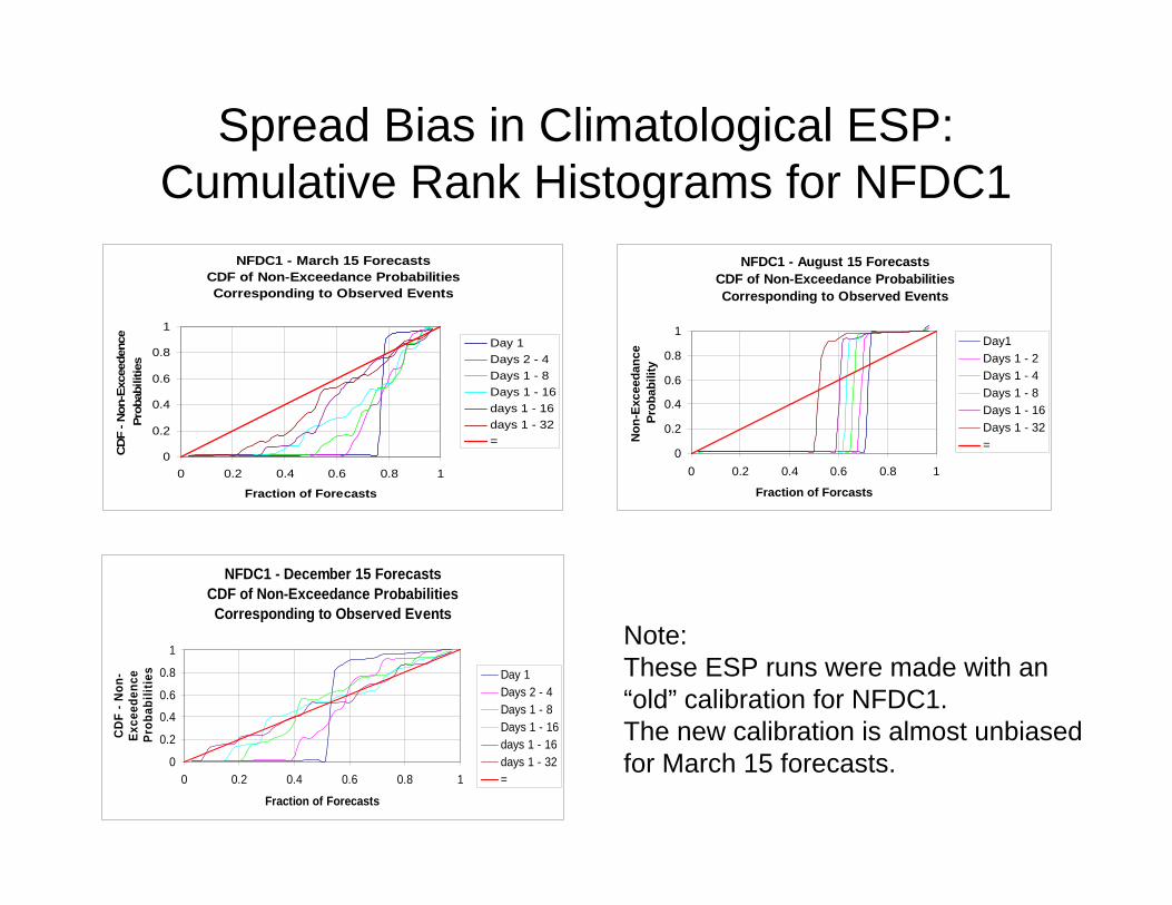
Spread Bias in Climatological ESP:Cumulative Rank Histograms for NFDC1
NFDC1 - March 15 Forecasts CDF of Non-Exceedance ProbabilitiesCorresponding to Observed Events
0
0.2
0.4
0.6
0.8
1
0 0.2 0.4 0.6 0.8 1
Fraction of Forecasts
CD
F - N
on-E
xcee
denc
e Pr
obab
ilitie
s
Day 1Days 2 - 4Days 1 - 8Days 1 - 16days 1 - 16days 1 - 32=
NFDC1 - August 15 ForecastsCDF of Non-Exceedance ProbabilitiesCorresponding to Observed Events
0
0.2
0.4
0.6
0.8
1
0 0.2 0.4 0.6 0.8 1
Fraction of Forcasts
Non
-Exc
eeda
nce
Prob
abili
ty
Day1Days 1 - 2Days 1 - 4Days 1 - 8Days 1 - 16Days 1 - 32=
NFDC1 - December 15 Forecasts CDF of Non-Exceedance ProbabilitiesCorresponding to Observed Events
0
0.2
0.4
0.6
0.8
1
0 0.2 0.4 0.6 0.8 1
Fraction of Forecasts
CD
F - N
on-
Exce
eden
ce
Prob
abili
ties Day 1
Days 2 - 4Days 1 - 8Days 1 - 16days 1 - 16days 1 - 32=
Note:These ESP runs were made with an“old” calibration for NFDC1. The new calibration is almost unbiased for March 15 forecasts.

Hydrologic Ensemble Product Post-Processor
(to correct raw ESP bias and spread errors)Raw ESP
Streamflow Ensemble Products
Hydrologic Post-Processor(Accounts for uncertainty in
hydrologic model and in initial conditions)
Adjusted ESP Streamflow Ensemble Products
This post-processor operates on hydrologic “products” only. These products are derived for a “window” superimposed on an ensemble of ESP hydrographs. Within this window, the “product” is defined in terms of an “operation” on each hydrograph within the window. Example operations include: average, maximum, minimum, minimum of x-day average, volume in window, etc.
This post-processor DOES NOT adjust the raw ensemble time series members. It DOES produce adjusted values for the individual product members that:1. Preserves the “skill” of the raw ensemble forecast2. Removes mean bias3. Produces reliable probability forecasts

Hydrologic Post-Processor
• The ESP program generates an ensemble of streamflow forecasts that are conditioned on an ensemble of precipitation and temperature forecasts (i.e. ysim|fcst)
• These ESP forecasts assume that the initial conditions are known and that the hydrologic model is perfect
• The relationship between historical observations and simulations can be used to represent the uncertainty associated with the fact that the initial conditions are not known exactly and the model is imperfect (i.e. yobs|ysim)
• If we neglect the uncertainty in the relationship between yobs and ysim that is caused by the uncertainty in the estimated forcing used to generate ysimduring the forecast period, the pdf of yobs, given the ensemble of precipitation and temperature forecasts can be estimated by the relationship:
( ) ( ) ( ) dysimfcstysimfysimyobsffcstyobsf ∫+∞
=0
Adjusted ESP Forecast
Historical Simulation
Raw ESP Forecast
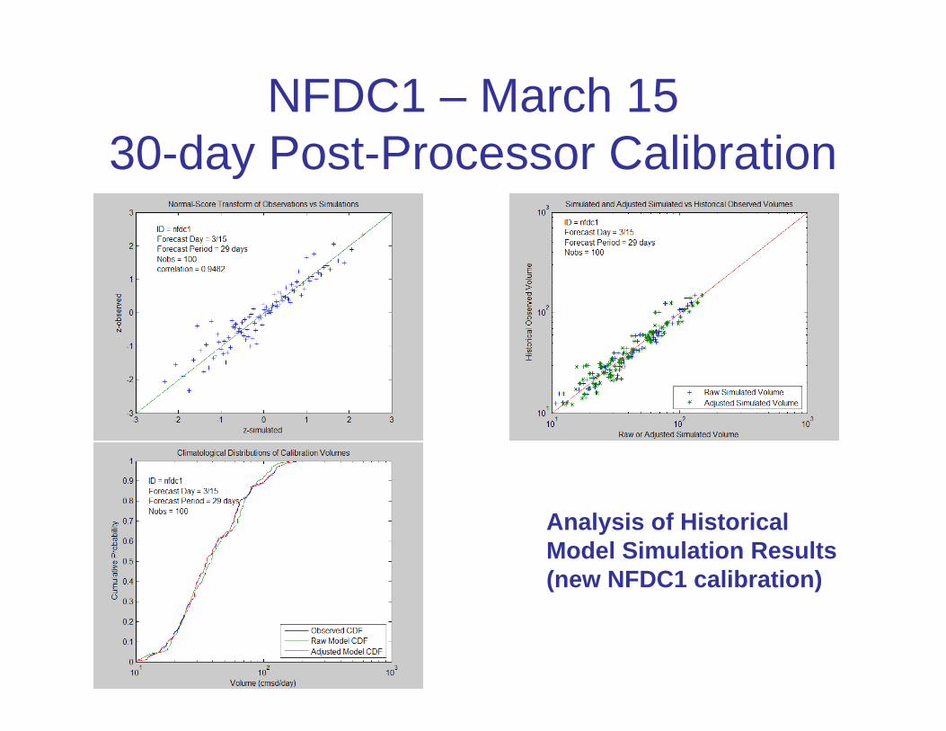
NFDC1 – March 15 30-day Post-Processor Calibration
Analysis of Historical Model Simulation Results(new NFDC1 calibration)

NFDC1 – March 1530-day GFS-Based
Hydrologic Ensemble Forecasts
Ensemble Mean vs Observed Cumulative Rank Histograms
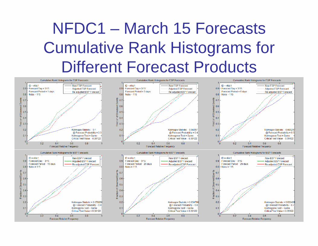
NFDC1 – March 15 ForecastsCumulative Rank Histograms for
Different Forecast Products

Cumulative Rank Histograms (NFDC1)December 15 Forecasts
Cumulative Rank Histogram - Day 1December 15 Forecasts
0
0.2
0.4
0.6
0.8
1
0 0.2 0.4 0.6 0.8 1
Forecast Probability
Obs
erve
d Pr
obab
ility
Raw ESPAdjusted ESP=
Cumulative Rank Histogram - Days 1-8December 15 Forecasts
0
0.2
0.4
0.6
0.8
1
0 0.2 0.4 0.6 0.8 1
Forecast Probability
Obs
erve
d Pr
obab
ility
Raw ESPAdjusted ESP=
Cumulative Rank Histogram - Days 1-32December 15 Forecasts
0
0.2
0.4
0.6
0.8
1
0 0.2 0.4 0.6 0.8 1
Forecast Probability
Obs
erve
d Pr
obab
ility
Raw ESPAdjusted ESP=
Cumulative Rank Histogram - Days 1-4December 15 Forecasts
0
0.2
0.4
0.6
0.8
1
0 0.2 0.4 0.6 0.8 1
Forecast Probability
Obs
erve
d Pr
obab
ility
Raw ESPAdjusted ESP=

GLDA3(Lake Powell Inflow)
EPG Post-Processor Calibration Results
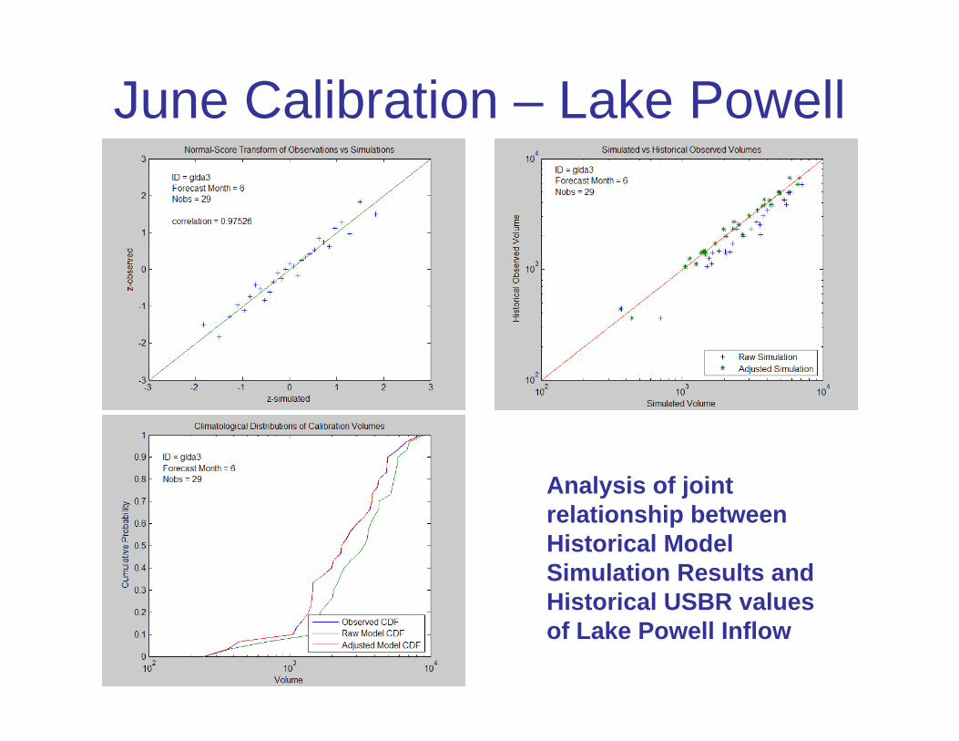
June Calibration – Lake Powell
Analysis of joint relationship between Historical Model Simulation Results and Historical USBR values of Lake Powell Inflow

Recent June Forecasts
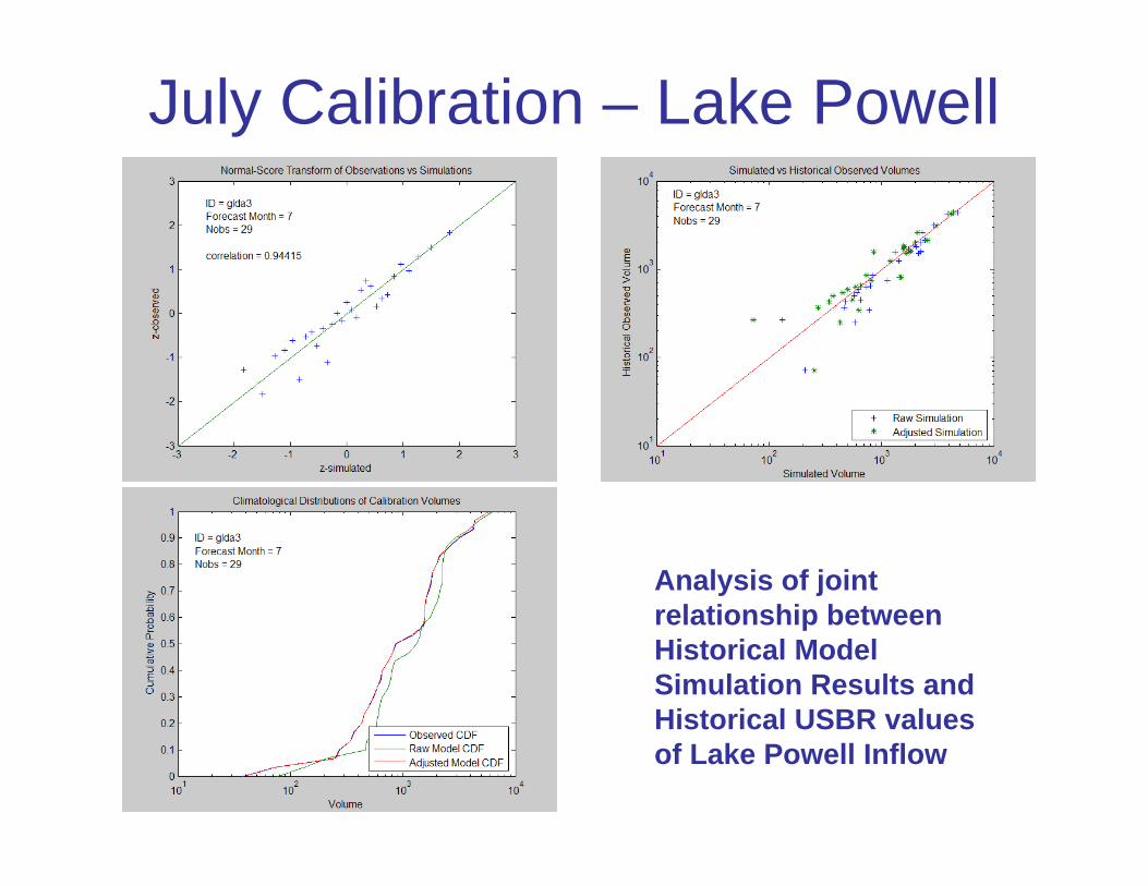
July Calibration – Lake Powell
Analysis of joint relationship between Historical Model Simulation Results and Historical USBR values of Lake Powell Inflow

Recent July Forecasts

LAMC1(Lake Mendocino, CA)
Russian River Basin

CREC1 – R0G14C30
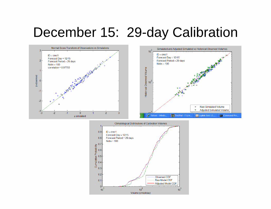
December 15: 29-day Calibration
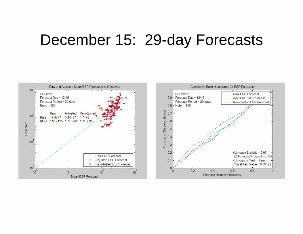
December 15: 29-day Forecasts

December 15: 10-day Calibration

December 15: 10-day Forecasts
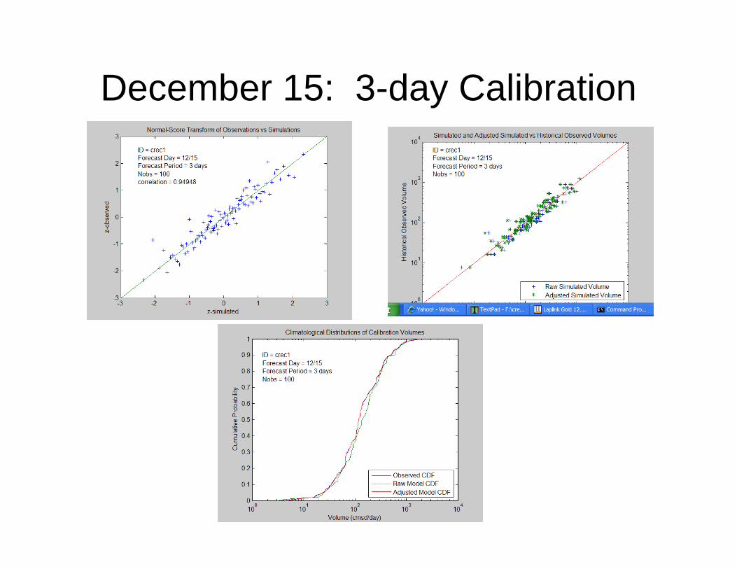
December 15: 3-day Calibration
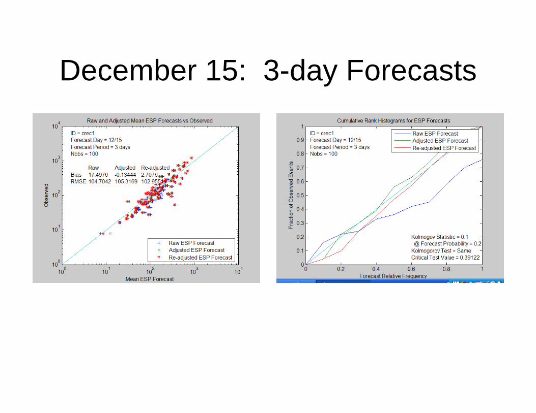
December 15: 3-day Forecasts
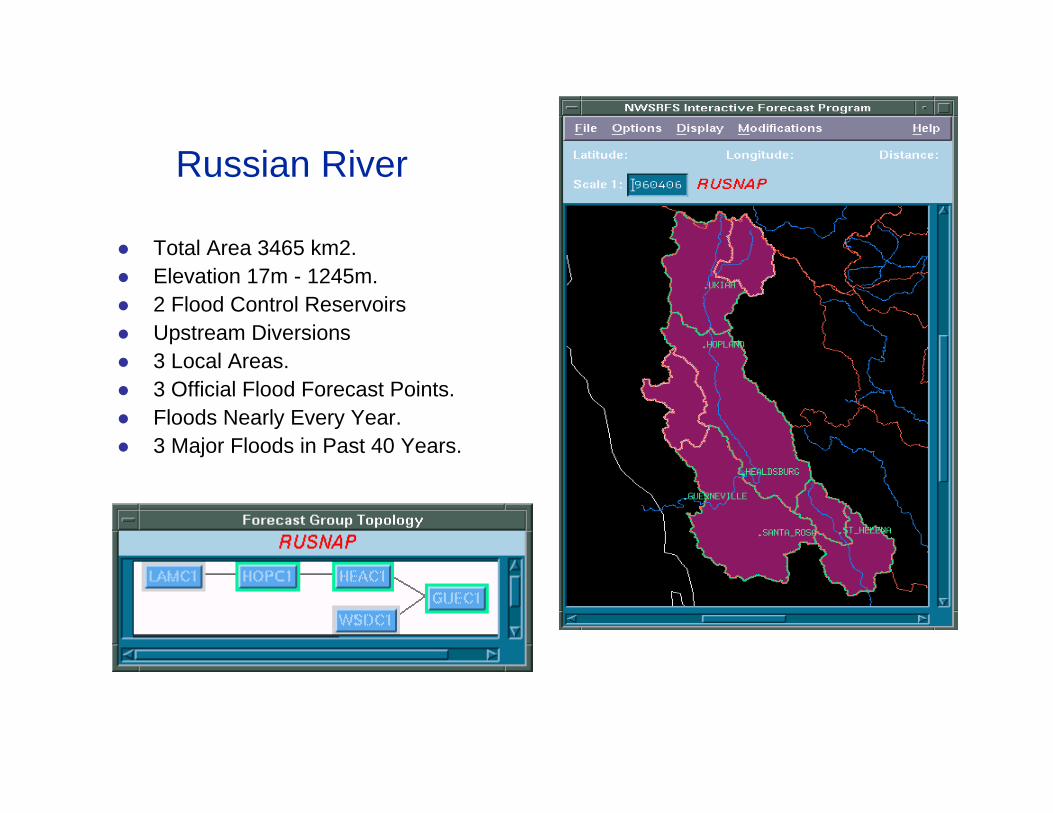
Total Area 3465 km2. Elevation 17m - 1245m.2 Flood Control ReservoirsUpstream Diversions3 Local Areas.3 Official Flood Forecast Points.Floods Nearly Every Year.3 Major Floods in Past 40 Years.
Russian River
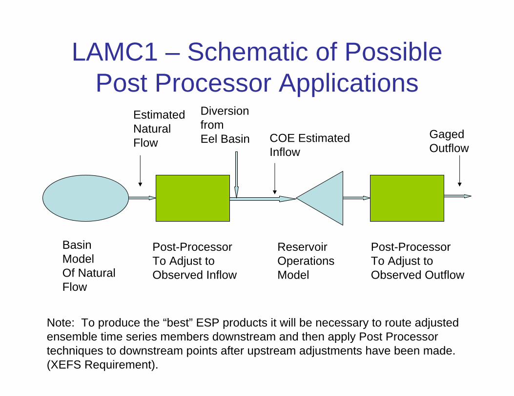
LAMC1 – Schematic of Possible Post Processor Applications
BasinModelOf NaturalFlow
Post-ProcessorTo Adjust toObserved Inflow
Reservoir OperationsModel
Post-ProcessorTo Adjust toObserved Outflow
GagedOutflow
COE EstimatedInflow
Diversion fromEel Basin
EstimatedNaturalFlow
Note: To produce the “best” ESP products it will be necessary to route adjusted ensemble time series members downstream and then apply Post Processor techniques to downstream points after upstream adjustments have been made. (XEFS Requirement).

Full Natural Flow – March 15
Analysis of Historical Model Simulation Results of Full Natural Flow
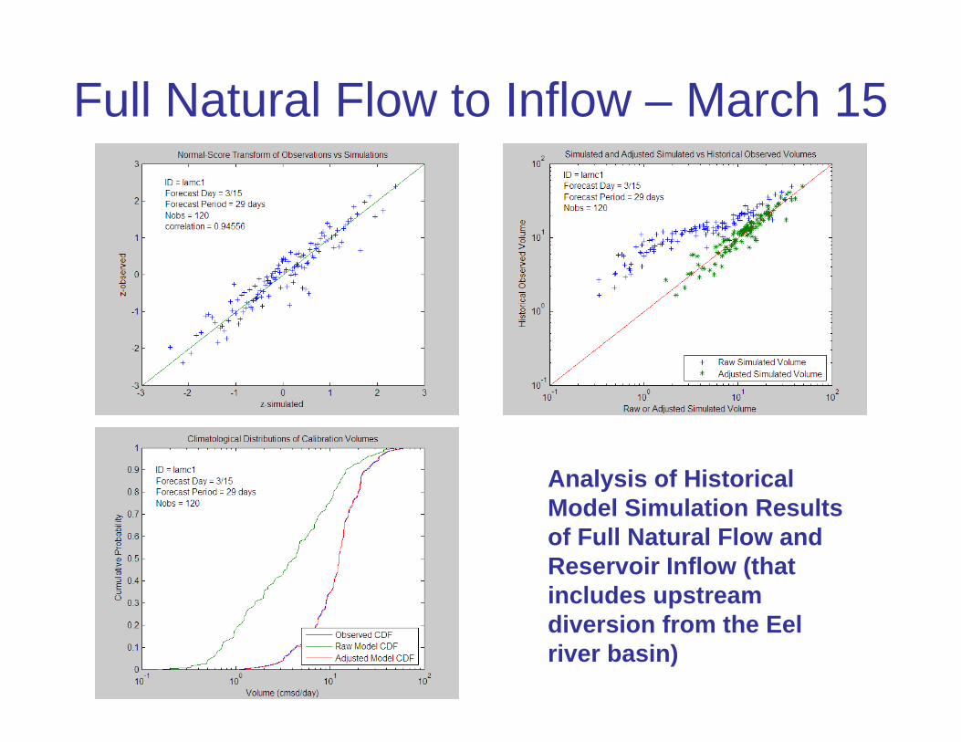
Full Natural Flow to Inflow – March 15
Analysis of Historical Model Simulation Results of Full Natural Flow and Reservoir Inflow (that includes upstream diversion from the Eel river basin)

Climatologies of Measured Inflow and Modeled Natural Flow (December – June)

Full Natural Inflow to ResevoirOutflow - March 15
Analysis of Joint Relationship between Historical Model Simulation Results of Full Natural Flow and Observed Reservoir Outflow
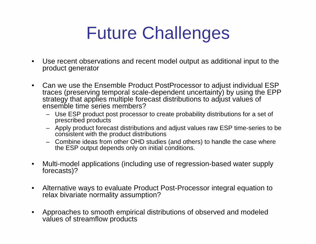
Future Challenges• Use recent observations and recent model output as additional input to the
product generator
• Can we use the Ensemble Product PostProcessor to adjust individual ESP traces (preserving temporal scale-dependent uncertainty) by using the EPP strategy that applies multiple forecast distributions to adjust values of ensemble time series members?
– Use ESP product post processor to create probability distributions for a set of prescribed products
– Apply product forecast distributions and adjust values raw ESP time-series to be consistent with the product distributions
– Combine ideas from other OHD studies (and others) to handle the case where the ESP output depends only on initial conditions.
• Multi-model applications (including use of regression-based water supply forecasts)?
• Alternative ways to evaluate Product Post-Processor integral equation to relax bivariate normality assumption?
• Approaches to smooth empirical distributions of observed and modeled values of streamflow products

ESP Time-Series Postprocessor Possible Science Strategy
• Two Step Process– Use ESP Product Post-Processor to create updated
probability distributions of forecast “products”– Use “Schaake Shuffle” to create ensemble members
that “preserve” all product probability distributions
Raw ESP Forecasts:
HMOS short-termESP traces
Use ESP ProductPost Processor
To createForecast Probability
Distributions
Control FileDefines
“ESP Products”
Adjust Raw ESP and
HMOS time series to
Preserve ProductProbability
Distributions
Raw ESP Forecasts,Recent Observations,Recent Model Output: Adjusted
ESP Time Series:

Thank You
Related Documents