A Polymorphic Dynamic Network Loading Model

Computer-Aided Civil and Infrastructure Engineering 23 (2008) 86–103

A Polymorphic Dynamic Network Loading Model

Yu (Marco) Nie∗

Department of Civil and Environmental Engineering, Northwestern University

&

Jingtao Ma & H. Michael Zhang†

Department of Civil and Environmental Engineering, University of California, Davis, CA, USA

Abstract: A polymorphic dynamic network loading(PDNL) model is developed and discretized to integratea variety of macroscopic traffic flow and node models.The polymorphism, realized through a general node-linkinterface and proper discretization, offers several promi-nent advantages. First of all, PDNL allows road facilitiesin the same network to be represented by different traf-fic flow models based on the tradeoff of efficiency andrealism and/or the characteristics of the targeted prob-lem. Second, new macroscopic link/node models can beeasily plugged into the framework and compared againstexisting ones. Third, PDNL decouples links and nodesin network loading, and thus opens the door to parallelcomputing. Finally, PDNL keeps track of individual ve-hicular quanta of arbitrary size, which makes it possibleto replicate analytical loading results as closely as desired.PDNL, thus, offers an ideal platform for studying both an-alytical dynamic traffic assignment problems of differentkinds and macroscopic traffic simulation.

1 INTRODUCTION

Dynamic network loading (DNL) is an underlying com-ponent of many dynamic network problems in whichpath costs depend on temporal path flows in ways gov-erned by traffic propagation and interaction. In the past

†CKS Professor, Tongji University, Shanghai, China.∗To whom correspondence should be addressed. E-mail: [email protected].

two decades, DNL has been extensively studied owingto the needs of simulating urban traffic and solving dy-namic traffic assignment (DTA) problems. In this articlewe are concerned with the following DNL problem:

Definition 1 (Dynamic Network Loading): The DNLproblem determines, on a congested network and overa fixed time period, link cumulative arrival/departurecurves (hence time-dependent link/path travel times) cor-responding to a given set of temporal path flow rates.

In other words, DNL represents a mapping from pathinflows to experienced travel times on the paths. Ac-cording to how they model traffic propagation and inter-action, existing DNL models may be classified into threegroups: macroscopic, microscopic, and mesoscopic mod-els. Providing a complete list of all existing DNL mod-els/packages is difficult. Table 1 attempts to cover thebest-known works in each of the three categories.1

Although microscopic models provide the most de-tailed representation of traffic, they share two majorlimitations: the curse of high computational overhead,which often prohibits large-scale applications, and theanalytical intractability often inherited from the MonteCarlo nature of the models. We are not suggesting, how-ever, that macroscopic models can solve the DNL prob-lem “analytically.” Indeed, even with the simplest as-sumptions, the mapping from path flow to path coststill cannot be cast in a closed form for general net-works. Nevertheless, for macroscopic models, analyticalformulas for such a mapping may be obtained for spe-cial networks (e.g., with a single or two tandem links).

C© 2008 Computer-Aided Civil and Infrastructure Engineering. Published by Blackwell Publishing, 350 Main Street, Malden, MA 02148, USA,and 9600 Garsington Road, Oxford OX4 2DQ, UK.

PDNL model 87

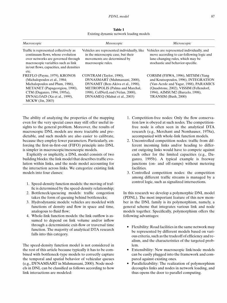
Table 1Existing dynamic network loading models

Macroscopic Mesoscopic Microscopic

Traffic is represented collectively ascontinuum flows, whose evolutionover networks are governed throughmacroscopic variables such as linkin/out flows, capacities, and densitiesetc.

Vehicles are represented individually, likein the microscopic case, but theirmovements are determined bymacroscopic rules.

Vehicles are represented individually, andmove according to car-following logic andlane-changing rules, which may bestochastic and behavior-specific.

FREFLO (Payne, 1979), KRONOS(Michalopoulos et al., 1984;Michalopoulos and Plum, 1986),METANET (Papageorgiou, 1990),CTM (Daganzo, 1994, 1995a),DYNALOAD (Xu et al., 1999),MCKW (Jin, 2003)

CONTRAM (Taylor, 1990),DYNASMART (Mahmassani, 2000),DYNAMIT (Ben-Akiva et al., 1998),METROPOLIS (Palma and Marchal,1998), CellNetLoad (Velan, 2000),DYNAMEQ (Mahut et al., 2003)

CORSIM (FHWA, 1996), MITSIM (Yangand Koutsopoulos, 1996), INTEGRATION(Van-Aerde and Yagar, 1988), PARAMICS(Quadstone, 2002), VISSIM (Fellendorf,1994), AIMSUM2 (Barcelo, 1998),TRANSIM (Bush, 2000)

The ability of analyzing the properties of the mappingeven for the very special cases may still offer useful in-sights to the general problem. Moreover, the results ofmacroscopic DNL models are more tractable and pre-dictable, and such models are also easier to calibrate,because they employ fewer parameters. Particularly, en-forcing the first-in-first-out (FIFO) principle into DNLis simpler in macroscopic/mesoscopic models.

Explicitly or implicitly, a DNL model consists of twobuilding blocks: the link model that describes traffic evo-lution within links, and the node model accounting forthe interaction across links. We categorize existing linkmodels into four classes:

1. Speed-density function models: the moving of traf-fic is determined by the speed-density relationship;

2. Bottleneck/queueing models: traffic congestiontakes the form of queuing behind bottlenecks;

3. Hydrodynamic models: vehicles are modeled withfunctions of density and flow in space and time,analogous to fluid flow;

4. Whole-link function models: the link outflow is as-sumed to depend on link volume and/or inflowthrough a deterministic exit-flow or traversal timefunction. The majority of analytical DTA researchfalls into this category.

The speed-density function model is not considered inthe rest of this article because typically it has to be com-bined with bottleneck-type models to correctly capturethe temporal and spatial behavior of vehicular queues(e.g., DYNAMSART in Mahmassani, 2000). Node mod-els in DNL can be classified as follows according to howlink interactions are modeled:

1. Competition-free nodes: Only the flow conserva-tion law is obeyed at such nodes. The competition-free node is often seen in the analytical DTAresearch (e.g., Merchant and Nemhauser, 1978a),accompanied with whole-link function models.

2. Uncontrolled competition nodes: traffic from dif-ferent incoming links and/or heading to differ-ent outgoing links would have to compete againsteach other for the limited capacities (e.g., Da-ganzo, 1995b). A typical example is freewayjunctions (on- and off-ramps) without meteringfacilities.

3. Controlled competition nodes: the competitionamong different traffic streams is managed by acontrol logic, such as signalized intersections.

In this research we develop a polymorphic DNL model(PDNL). The most important feature of this new mem-ber in the DNL family is its polymorphism, namely, ageneral scheme that integrates various link and nodemodels together. Specifically, polymorphism offers thefollowing advantages:

� Flexibility: Road facilities in the same network maybe represented by different models based on vari-ous criteria, such as the tradeoff of efficiency and re-alism, and the characteristics of the targeted prob-lem.

� Extensibility: New macroscopic link/node modelscan be easily plugged into the framework and com-pared against existing ones.

� Parallelizability: The realization of polymorphismdecouples links and nodes in network loading, andthus opens the door to parallel computing.

88 Nie, Ma & Zhang

The PDNL model takes a mesoscopic approach to traceindividual vehicular quanta. A vehicular quantum is anindivisible flow element that is treated in PDNL like a ve-hicle in microscopic simulation. However the size of ve-hicular quanta can be set arbitrarily small, which makes itpossible to replicate analytical loading results as closelyas desired, whenever a need to compare numerical andanalytical results arises. Section 4.2 explains in detail whythe size of quanta is important to the stability of load-ing results. In a nutshell, PDNL offers a desirable toolfor studying both DTA problems of different kinds andmacroscopic traffic simulation.

The next section briefly reviews analytical link mod-els. Section 3 presents a node model for general inter-sections. Section 4 discusses the discretization schemeand the realization of polymorphism, and how the FIFObehavior is enforced. Numerical results are reported inSection 6, and Section 7 concludes the article.

2 LINK MODELS

This section reviews bottleneck, whole-link function, andhydrodynamic models. Each link is assumed to be ho-mogenous, i.e., the road characteristics remain the sameeverywhere in a link.

2.1 Bottleneck models

In bottleneck-type models, vehicles always move alonga link at the free-flow speed before they arrive at the exitnode, where they form a FIFO queue if the outflow ratethey induce exceeds the maximum discharge rate (bot-tleneck capacity) of the link. A continuous mathematicalform reads

dλ

dt=

{0 if λ(t) = 0 and u(t − τ0) < C

u(t − τ0) − C otherwise(1)

τ (t) = τ0 + λ(t + τ0)/C (2)

where u(t) is the entry rate at time t; λ is the total numberof queuing vehicles at the exit node; τ 0 is the free flowtravel time; τ (t) is the link traversal time correspondingto the entry time t; and C is the bottleneck capacity.

A bottleneck model that ignores the physical lengthof vehicles is called a point-queue (P-Q) model, whichnever predicts a queue spillback. To allow spillback, asimple remedy is to block inflow whenever the followingcondition is met:

Cl ≥∫ t

0u(w) dw −

∫ t

0v(w) dw, ∀t (3)

where Cl is the holding capacity, i.e., the maximum num-ber of vehicles that a link can accommodate; v(t) is theexit rate at time t.

We call a bottleneck model equipped with the condi-tion (3) a spatial-queue (S-Q) model. Although the S-Qmodel captures the propagation of queues across links,it presumes that any queue is at jam density (Zhang andNie, 2006), which does not accord with existing empiri-cal evidence. We note that the S-Q model may be viewedas a simplified formulation of Newell’s trilogy (Newell,1993), which was later shown to be fully equivalent tothe LWR model for triangle fundamental diagrams (Da-ganzo, 2005b).

2.2 Whole-link function models

In general this class of models trade traffic realism withanalytical tractability. The earliest known example, dueto the pioneering work of Merchant and Nemhauser(1978a, 1978b), is the exit-flow model. This model as-sumes that the link exit flow rate at any time is a non-decreasing and concave function of current link volume,i.e.,

dx(t)dt

= u(t) − v(t) (4)

v(t) = ge(x(t)) ≤ x(t) (5)

where x(t) is the link volume at time t; ge(·) is the linkexit flow function.

Equation (4) expresses the flow conservation condi-tion, i.e., the net change of link volume equals the dif-ference between inflow and outflow rates. The exit-flowmodel has been extensively used for studying DTA prob-lems.

Another widely used model in this category is a directextension of the static link performance function (e.g.,Friesz et al., 1993; Astarita, 1996; Carey and McCartney,2002). Known as the delay-function model, it assumesthat τ (t), the actual traverse time experienced by travel-ers entering a link at t, is a function of the link volumex(t). The model reads

dx(t)dt

= u(t) − v(t) (6)

τ (t) = gd(x(t)) (7)

v(t + τ (t)) = u(t)1 + τ̇ (t)

(8)

PDNL model 89

where gd(·) denotes the delay function. Equation (8)(see, e.g., Astarita, 1996) ensures the FIFO behavior byforcing vehicles that enter the link at t to be pushed outat t + τ (t).

Carey and Ge (2005) showed that the delay functionmodel converges to the LWR model on a single link whenthe length of discrete segments approaches zero. How-ever, in general the whole link model lacks a mechanismto capture the backward shockwaves, which makes it dif-ficult to reflect vehicular queuing in a realistic way. It isestablished (Friesz et al., 1993; Daganzo, 1995b; Careyand McCartney, 2002) that any affine function can guar-antee FIFO in the delay-function model. Whether or notthere exists any nonlinear functional form that ensuresFIFO, however, remains an unresolved issue. Xu et al.(1999) gave an example of FIFO violation when the de-lay function is quadratic.

2.3 Hydrodynamic models

Hydrodynamic models view traffic as a continuous fluidrepresented by density (k), speed (s), and flow-rate(q). They are also known as kinematic wave models(KW) because their solutions can be characterized bycombinations of kinematic waves in either of the threequantities. The movement of traffic on a homogeneouslink is governed by the following flow conservationlaw:

∂q∂x

+ ∂k∂t

= 0 (9)

where x and t denote space and time, respectively. Afundamental assumption in hydrodynamic models is thatthe flow rate q is a function of traffic density k, i.e.,

q = F(k) (10)

Combining (10) into (9) yields the KW model of trafficflow, which is widely known as the LWR model (Lighthilland Whitham, 1955; Richards, 1956):

q̇∂k∂x

+ ∂k∂t

= 0, q̇ = ∂ F∂k

(11)

The LWR model can be solved numerically by the fi-nite difference method such as the first-order Gudunovscheme (Godunov, 1959). For the triangle fundamen-tal diagram, Daganzo (1994) proposed a streamlinedscheme known as the cell transmission model (CTM).Luke (1972) and Newell (1993) showed that, in a sys-tem governed by the one-dimensional conversation lawsuch as the LWR model, cumulative counts at any space-time point is the lower-envelope of those derived fromboundary conditions. This result was recently formalizedby Daganzo (2005a, 2005b) as a variational formulationof the KW model. The Luke–Newell–Daganzo (LND)

theory of traffic flow can generate exact wave solutionsfor the triangle fundamental diagram (Daganzo, 2005b).This latest development is not included in this study, how-ever, because the corresponding node models are yet tobe developed.

3 NODE MODELS

This section only considers nodes with competition. Thefree-competition node is not further discussed becauseits model is flow conservation.

Following Daganzo (1995a), this section first examinesthe diverge and merge on freeways, and then extends togeneral intersections. Let us first define the demand andsupply of a link.

Definition 2 (Link Demand and Supply): The demand ofa link, D, is the maximum possible exit flow rate, i.e.,

D = min{C, Q},

the supply of a link, S, is the maximum possible receivingflow rate, i.e.,

S = min{C, R}

where C is the flow capacity depending on road charac-teristics and/or control strategies; Q is the rate of the flowthat is ready to exit; R is the maximum entry flow rate tothe link permitted by the current traffic condition.

How R may be computed determines largely thebehavior of queue spillback and varies in differentlink models. We will discuss this in detail in the nextsection.

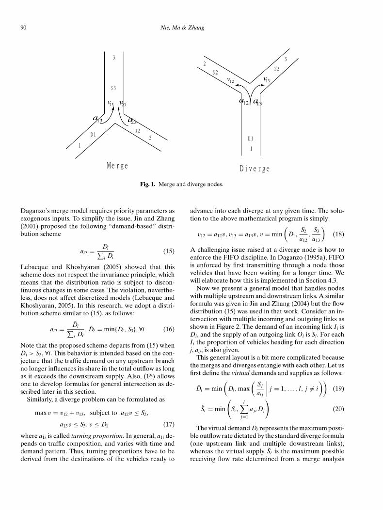
A merge problem can be formulated as a maximiza-tion problem as follows (see Figure 1)

max v =∑

i

vi3, subject to 0 ≤ vi3 ≤ Di , i = 1, 2,

∑i

vi3 ≤ S3 (12)

where Di is the demand of link i , i = 1, 2. S3 is the supplyof link 3.

The solution to this problem has the following simplestructure:

vi3 = ai3v, ∀i, v = min{D1 + D2, S3} (13)

where ai3, ∀i is called distribution ratio. Daganzo (1995a)suggested that ai3 is proportional to some priority pa-rameters pi3 (which is determined by geometry designand other properties),

ai3

pi3= constant ∀i,

∑i

pi3 = 1 (14)

90 Nie, Ma & Zhang

13v

13v12v

13a12a23v

13a23a

Fig. 1. Merge and diverge nodes.

Daganzo’s merge model requires priority parameters asexogenous inputs. To simplify the issue, Jin and Zhang(2001) proposed the following “demand-based” distri-bution scheme

ai3 = Di∑i Di

(15)

Lebacque and Khoshyaran (2005) showed that thisscheme does not respect the invariance principle, whichmeans that the distribution ratio is subject to discon-tinuous changes in some cases. The violation, neverthe-less, does not affect discretized models (Lebacque andKhoshyaran, 2005). In this research, we adopt a distri-bution scheme similar to (15), as follows:

ai3 = D̃i∑i D̃i

, D̃i = min{Di , S3}, ∀i (16)

Note that the proposed scheme departs from (15) whenDi > S3, ∀i. This behavior is intended based on the con-jecture that the traffic demand on any upstream branchno longer influences its share in the total outflow as longas it exceeds the downstream supply. Also, (16) allowsone to develop formulas for general intersection as de-scribed later in this section.

Similarly, a diverge problem can be formulated as

max v = v12 + v13, subject to a12v ≤ S2,

a13v ≤ S3, v ≤ D1 (17)

where a1i is called turning proportion. In general, a1i de-pends on traffic composition, and varies with time anddemand pattern. Thus, turning proportions have to bederived from the destinations of the vehicles ready to

advance into each diverge at any given time. The solu-tion to the above mathematical program is simply

v12 = a12v, v13 = a13v, v = min(

D1,S2

a12,

S3

a13

)(18)

A challenging issue raised at a diverge node is how toenforce the FIFO discipline. In Daganzo (1995a), FIFOis enforced by first transmitting through a node thosevehicles that have been waiting for a longer time. Wewill elaborate how this is implemented in Section 4.3.

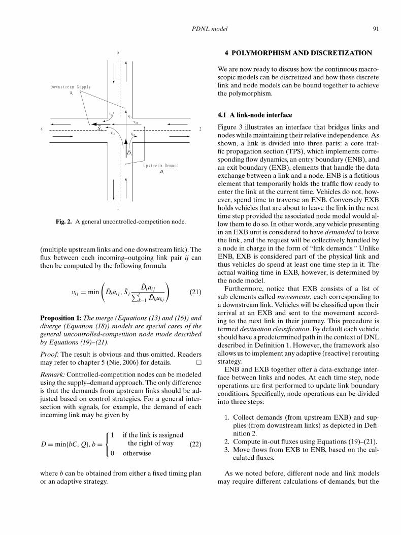
Now we present a general model that handles nodeswith multiple upstream and downstream links. A similarformula was given in Jin and Zhang (2004) but the flowdistribution (15) was used in that work. Consider an in-tersection with multiple incoming and outgoing links asshown in Figure 2. The demand of an incoming link Ii isDi, and the supply of an outgoing link Oi is Si. For eachIi the proportion of vehicles heading for each directionj, aij, is also given.

This general layout is a bit more complicated becausethe merges and diverges entangle with each other. Let usfirst define the virtual demands and supplies as follows:

D̃i = min(

Di , max(

Sj

ai j

∣∣∣∣ j = 1, . . . , l, j = i))

(19)

S̃i = min

(Si ,

l∑j=1

a ji Dj

)(20)

The virtual demand D̃i represents the maximum possi-ble outflow rate dictated by the standard diverge formula(one upstream link and multiple downstream links),whereas the virtual supply S̃i is the maximum possiblereceiving flow rate determined from a merge analysis

PDNL model 91

iS

iD

1

~D

4

~S

13v

14v12v

24v

34v

Fig. 2. A general uncontrolled-competition node.

(multiple upstream links and one downstream link). Theflux between each incoming–outgoing link pair ij canthen be computed by the following formula

vi j = min

(D̃i ai j , S̃ j

D̃i ai j∑lk=1 D̃kakj

)(21)

Proposition 1: The merge (Equations (13) and (16)) anddiverge (Equation (18)) models are special cases of thegeneral uncontrolled-competition node mode describedby Equations (19)–(21).

Proof: The result is obvious and thus omitted. Readersmay refer to chapter 5 (Nie, 2006) for details. �Remark: Controlled-competition nodes can be modeledusing the supply–demand approach. The only differenceis that the demands from upstream links should be ad-justed based on control strategies. For a general inter-section with signals, for example, the demand of eachincoming link may be given by

D = min{bC, Q}, b =

1 if the link is assignedthe right of way

0 otherwise(22)

where b can be obtained from either a fixed timing planor an adaptive strategy.

4 POLYMORPHISM AND DISCRETIZATION

We are now ready to discuss how the continuous macro-scopic models can be discretized and how these discretelink and node models can be bound together to achievethe polymorphism.

4.1 A link-node interface

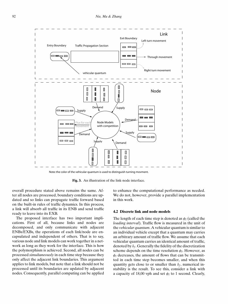
Figure 3 illustrates an interface that bridges links andnodes while maintaining their relative independence. Asshown, a link is divided into three parts: a core traf-fic propagation section (TPS), which implements corre-sponding flow dynamics, an entry boundary (ENB), andan exit boundary (EXB), elements that handle the dataexchange between a link and a node. ENB is a fictitiouselement that temporarily holds the traffic flow ready toenter the link at the current time. Vehicles do not, how-ever, spend time to traverse an ENB. Conversely EXBholds vehicles that are about to leave the link in the nexttime step provided the associated node model would al-low them to do so. In other words, any vehicle presentingin an EXB unit is considered to have demanded to leavethe link, and the request will be collectively handled bya node in charge in the form of “link demands.” UnlikeENB, EXB is considered part of the physical link andthus vehicles do spend at least one time step in it. Theactual waiting time in EXB, however, is determined bythe node model.

Furthermore, notice that EXB consists of a list ofsub elements called movements, each corresponding toa downstream link. Vehicles will be classified upon theirarrival at an EXB and sent to the movement accord-ing to the next link in their journey. This procedure istermed destination classification. By default each vehicleshould have a predetermined path in the context of DNLdescribed in Definition 1. However, the framework alsoallows us to implement any adaptive (reactive) reroutingstrategy.

ENB and EXB together offer a data-exchange inter-face between links and nodes. At each time step, nodeoperations are first performed to update link boundaryconditions. Specifically, node operations can be dividedinto three steps:

1. Collect demands (from upstream EXB) and sup-plies (from downstream links) as depicted in Defi-nition 2.

2. Compute in-out fluxes using Equations (19)–(21).3. Move flows from EXB to ENB, based on the cal-

culated fluxes.

As we noted before, different node and link modelsmay require different calculations of demands, but the

92 Nie, Ma & Zhang

Entry Boundary

Exit Boundary

Traffic Propagation Section

Left turn movement

Right turn movement

Through movement

Node Models with competition

Demand

Demand

Demand

Demand

SupplySupply

Supply

Supply

Flux for each movement

Node

Link

Note: the color of the vehicular quantum is used to distinguish turning movment.

vehicular quantum

Fig. 3. An illustration of the link-node interface.

overall procedure stated above remains the same. Af-ter all nodes are processed, boundary conditions are up-dated and so links can propagate traffic forward basedon the built-in rules of traffic dynamics. In this process,a link will absorb all traffic in its ENB and send trafficready to leave into its EXB.

The proposed interface has two important impli-cations. First of all, because links and nodes aredecomposed, and only communicate with adjacentENBs/EXBs, the operations of each link/node are en-capsulated and independent of others. That is to say,various node and link models can work together in a net-work as long as they work for the interface. This is howthe polymorphism is achieved. Second, all nodes can beprocessed simultaneously in each time step because theyonly affect the adjacent link boundaries. This argumentapplies to link models, but note that a link should not beprocessed until its boundaries are updated by adjacentnodes. Consequently, parallel computing can be applied

to enhance the computational performance as needed.We do not, however, provide a parallel implementationin this work.

4.2 Discrete link and node models

The length of each time step is denoted as φl (called theloading interval). Traffic flow is measured in the unit ofthe vehicular quantum. A vehicular quantum is similar toan individual vehicle except that a quantum may carriesan arbitrary amount of traffic flow. We assume that eachvehicular quantum carries an identical amount of traffic,denoted by δf . Generally the fidelity of the discretizationscheme depends on the time resolution φl. However, asφl decreases, the amount of flows that can be transmit-ted in each time step becomes smaller, and when thisquantity gets close to or smaller than δf , numerical in-stability is the result. To see this, consider a link witha capacity of 18,00 vph and set φl to 1 second. Clearly,

PDNL model 93

........ ........

0 1 2 3 i-1 i i+1 L-1L

01v12v 23v

iiv ,1− 1, +iiv

ENB

EXB

TPS

ik

il

xδ

Fig. 4. Discretization of the LWR model.

no more than 0.5 vehicles should be moved through anygiven location on that link during each φl to respect thecapacity. However, if the δ f = 1 vehicle, the realizedcapacity could only alternate between 0 (no quantumis moved) or 3,600 vph (one quantum is moved). Suchsharp jumps can introduce not only instability, but alsounexpected shockwaves as shown in Nie (2006). Theseproblems, however, can be overcome by using a suffi-ciently small δf .

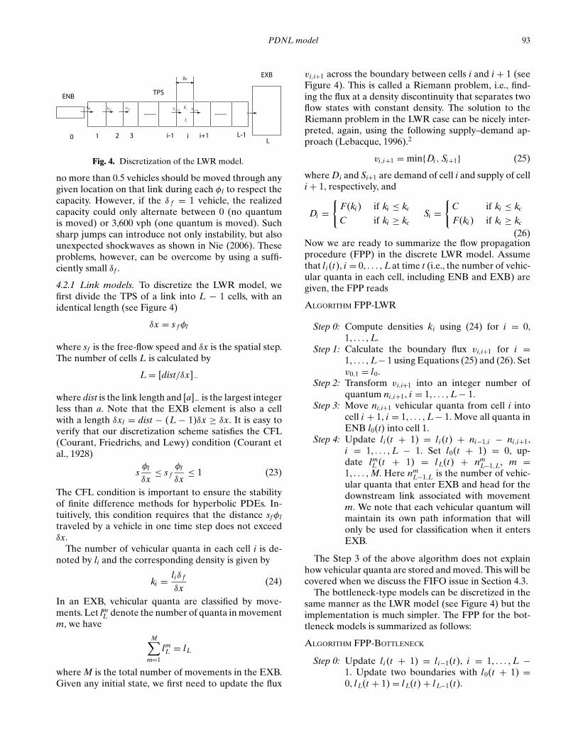
4.2.1 Link models. To discretize the LWR model, wefirst divide the TPS of a link into L − 1 cells, with anidentical length (see Figure 4)

δx = s f φl

where sf is the free-flow speed and δx is the spatial step.The number of cells L is calculated by

L = [dist/δx]−

where dist is the link length and [a]− is the largest integerless than a. Note that the EXB element is also a cellwith a length δxl = dist − (L − 1)δx ≥ δx. It is easy toverify that our discretization scheme satisfies the CFL(Courant, Friedrichs, and Lewy) condition (Courant etal., 1928)

sφl

δx≤ s f

φl

δx≤ 1 (23)

The CFL condition is important to ensure the stabilityof finite difference methods for hyperbolic PDEs. In-tuitively, this condition requires that the distance sf φl

traveled by a vehicle in one time step does not exceedδx.

The number of vehicular quanta in each cell i is de-noted by li and the corresponding density is given by

ki = liδ f

δx(24)

In an EXB, vehicular quanta are classified by move-ments. Let lmL denote the number of quanta in movementm, we have

M∑m=1

lmL = lL

where M is the total number of movements in the EXB.Given any initial state, we first need to update the flux

vi,i+1 across the boundary between cells i and i + 1 (seeFigure 4). This is called a Riemann problem, i.e., find-ing the flux at a density discontinuity that separates twoflow states with constant density. The solution to theRiemann problem in the LWR case can be nicely inter-preted, again, using the following supply–demand ap-proach (Lebacque, 1996).2

vi,i+1 = min{Di , Si+1} (25)

where Di and Si+1 are demand of cell i and supply of celli + 1, respectively, and

Di ={

F(ki ) if ki ≤ kc

C if ki ≥ kcSi =

{C if ki ≤ kc

F(ki ) if ki ≥ kc

(26)Now we are ready to summarize the flow propagationprocedure (FPP) in the discrete LWR model. Assumethat li (t), i = 0, . . . , Lat time t (i.e., the number of vehic-ular quanta in each cell, including ENB and EXB) aregiven, the FPP reads

ALGORITHM FPP-LWR

Step 0: Compute densities ki using (24) for i = 0,1, . . . , L.

Step 1: Calculate the boundary flux vi,i+1 for i =1, . . . , L− 1 using Equations (25) and (26). Setv0,1 = l0.

Step 2: Transform vi,i+1 into an integer number ofquantum ni,i+1, i = 1, . . . , L − 1.

Step 3: Move ni,i+1 vehicular quanta from cell i intocell i + 1, i = 1, . . . , L − 1. Move all quanta inENB l0(t) into cell 1.

Step 4: Update li (t + 1) = li (t) + ni−1,i − ni,i+1,i = 1, . . . , L − 1. Set l0(t + 1) = 0, up-date lm

L (t + 1) = l L(t) + nmL−1,L, m =

1, . . . , M. Here nmL−1,L is the number of vehic-

ular quanta that enter EXB and head for thedownstream link associated with movementm. We note that each vehicular quantum willmaintain its own path information that willonly be used for classification when it entersEXB.

The Step 3 of the above algorithm does not explainhow vehicular quanta are stored and moved. This will becovered when we discuss the FIFO issue in Section 4.3.

The bottleneck-type models can be discretized in thesame manner as the LWR model (see Figure 4) but theimplementation is much simpler. The FPP for the bot-tleneck models is summarized as follows:

ALGORITHM FPP-BOTTLENECK

Step 0: Update li (t + 1) = li−1(t), i = 1, . . . , L −1. Update two boundaries with l0(t + 1) =0, l L(t + 1) = l L(t) + l L−1(t).

94 Nie, Ma & Zhang

ENB

EXB

.......iet .......il

Floating cells

1iL

Earlier leaving time

TPS

0

L+1

Fig. 5. Discretization of the delay-function model.

Step 1: Move lL−1(t) vehicular quanta from ENB toEXB. That is, vehicular quanta are not actuallymoved from one cell to another as in the LWRmodel. Rather, they stay in ENB until theydirectly “jump” into EXB.

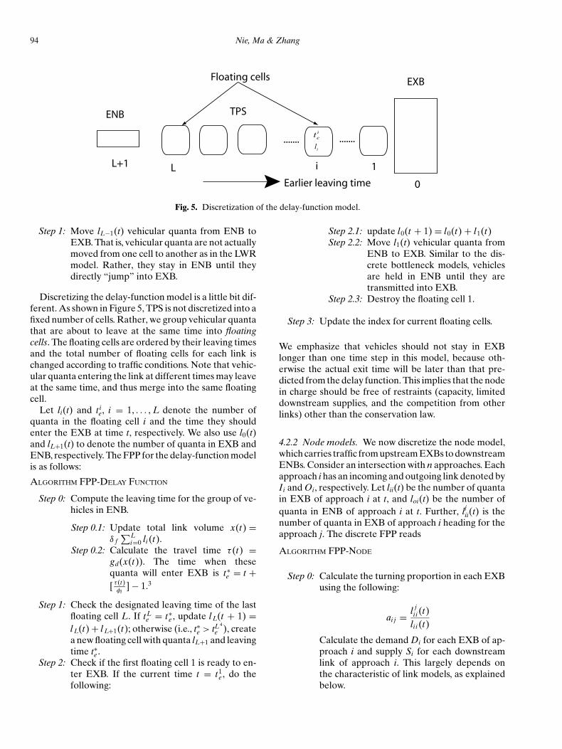
Discretizing the delay-function model is a little bit dif-ferent. As shown in Figure 5, TPS is not discretized into afixed number of cells. Rather, we group vehicular quantathat are about to leave at the same time into floatingcells. The floating cells are ordered by their leaving timesand the total number of floating cells for each link ischanged according to traffic conditions. Note that vehic-ular quanta entering the link at different times may leaveat the same time, and thus merge into the same floatingcell.

Let li(t) and t ie, i = 1, . . . , L denote the number of

quanta in the floating cell i and the time they shouldenter the EXB at time t, respectively. We also use l0(t)and lL+1(t) to denote the number of quanta in EXB andENB, respectively. The FPP for the delay-function modelis as follows:

ALGORITHM FPP-DELAY FUNCTION

Step 0: Compute the leaving time for the group of ve-hicles in ENB.

Step 0.1: Update total link volume x(t) =δ f

∑Li=0 li (t).

Step 0.2: Calculate the travel time τ (t) =gd(x(t)). The time when thesequanta will enter EXB is t∗

e = t +[ τ (t)

φl] − 1.3

Step 1: Check the designated leaving time of the lastfloating cell L. If tL

e = t∗e , update l L(t + 1) =

l L(t) + l L+1(t); otherwise (i.e., t∗e > tLe4), create

a new floating cell with quanta lL+1 and leavingtime t∗e .

Step 2: Check if the first floating cell 1 is ready to en-ter EXB. If the current time t = t1

e , do thefollowing:

Step 2.1: update l0(t + 1) = l0(t) + l1(t)Step 2.2: Move l1(t) vehicular quanta from

ENB to EXB. Similar to the dis-crete bottleneck models, vehiclesare held in ENB until they aretransmitted into EXB.

Step 2.3: Destroy the floating cell 1.

Step 3: Update the index for current floating cells.

We emphasize that vehicles should not stay in EXBlonger than one time step in this model, because oth-erwise the actual exit time will be later than that pre-dicted from the delay function. This implies that the nodein charge should be free of restraints (capacity, limiteddownstream supplies, and the competition from otherlinks) other than the conservation law.

4.2.2 Node models. We now discretize the node model,which carries traffic from upstream EXBs to downstreamENBs. Consider an intersection with n approaches. Eachapproach i has an incoming and outgoing link denoted byIi and Oi, respectively. Let lii(t) be the number of quantain EXB of approach i at t, and loi(t) be the number ofquanta in ENB of approach i at t. Further, ljii(t) is thenumber of quanta in EXB of approach i heading for theapproach j. The discrete FPP reads

ALGORITHM FPP-NODE

Step 0: Calculate the turning proportion in each EXBusing the following:

ai j = l ji i (t)

lii (t)

Calculate the demand Di for each EXB of ap-proach i and supply Si for each downstreamlink of approach i. This largely depends onthe characteristic of link models, as explainedbelow.

PDNL model 95

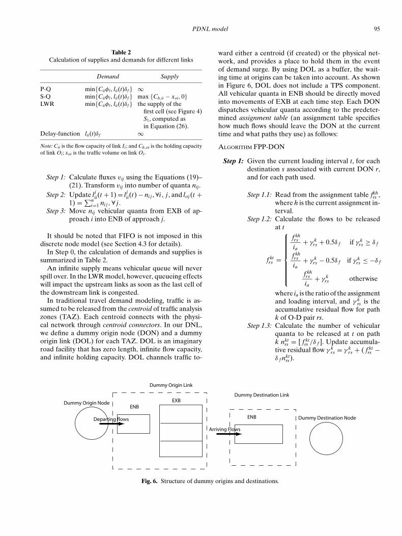
Table 2Calculation of supplies and demands for different links

Demand Supply

P-Q min{Ciiφl, lii(t)δf} ∞S-Q min{Ciiφl, lii(t)δf} max {Ch,ii − xoi, 0}LWR min{Ciiφl, lii(t)δf} the supply of the

first cell (see Figure 4)S1, computed asin Equation (26).

Delay-function lii(t)δf ∞Note: Cii is the flow capacity of link Ii; and Ch,oi is the holding capacityof link Oi; xoi is the traffic volume on link Oi.

Step 1: Calculate fluxes vij using the Equations (19)–(21). Transform vij into number of quanta nij.

Step 2: Update l jii(t + 1) = l j

ii(t) − ni j , ∀i , j , and loj (t +1) = ∑n

i=1 ni j , ∀ j .Step 3: Move nij vehicular quanta from EXB of ap-

proach i into ENB of approach j.

It should be noted that FIFO is not imposed in thisdiscrete node model (see Section 4.3 for details).

In Step 0, the calculation of demands and supplies issummarized in Table 2.

An infinite supply means vehicular queue will neverspill over. In the LWR model, however, queueing effectswill impact the upstream links as soon as the last cell ofthe downstream link is congested.

In traditional travel demand modeling, traffic is as-sumed to be released from the centroid of traffic analysiszones (TAZ). Each centroid connects with the physi-cal network through centroid connectors. In our DNL,we define a dummy origin node (DON) and a dummyorigin link (DOL) for each TAZ. DOL is an imaginaryroad facility that has zero length, infinite flow capacity,and infinite holding capacity. DOL channels traffic to-

Dummy Origin Node

Dummy Origin Link

ENBEXB

Dummy Destination Link

ENB Dummy Destination NodeDeparting flows

Arriving Flows

Fig. 6. Structure of dummy origins and destinations.

ward either a centroid (if created) or the physical net-work, and provides a place to hold them in the eventof demand surge. By using DOL as a buffer, the wait-ing time at origins can be taken into account. As shownin Figure 6, DOL does not include a TPS component.All vehicular quanta in ENB should be directly movedinto movements of EXB at each time step. Each DONdispatches vehicular quanta according to the predeter-mined assignment table (an assignment table specifieshow much flows should leave the DON at the currenttime and what paths they use) as follows:

ALGORITHM FPP-DON

Step 1: Given the current loading interval t, for eachdestination s associated with current DON r,and for each path used.

Step 1.1: Read from the assignment table fkhrs ,

where h is the current assignment in-terval.

Step 1.2: Calculate the flows to be releasedat t

f ktrs =

f khrs

ia+ γ k

rs + 0.5δ f if γ krs ≥ δ f

f khrs

ia+ γ k

rs − 0.5δ f if γ krs ≤ −δ f

f khrs

ia+ γ k

rs otherwise

where ia is the ratio of the assignmentand loading interval, and γ k

rs is theaccumulative residual flow for pathk of O-D pair rs.

Step 1.3: Calculate the number of vehicularquanta to be released at t on pathk nkt

rs = [ f ktrs /δ f ]. Update accumula-

tive residual flow γ krs = γ k

rs + ( f ktrs −

δ f nktrs).

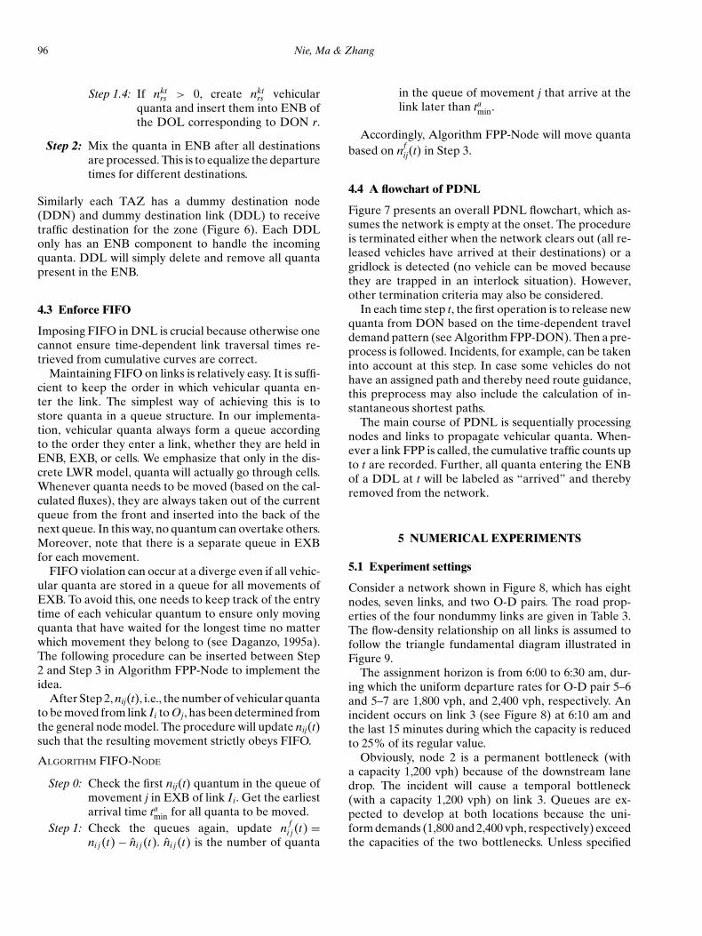
96 Nie, Ma & Zhang

Step 1.4: If nktrs > 0, create nkt

rs vehicularquanta and insert them into ENB ofthe DOL corresponding to DON r.

Step 2: Mix the quanta in ENB after all destinationsare processed. This is to equalize the departuretimes for different destinations.

Similarly each TAZ has a dummy destination node(DDN) and dummy destination link (DDL) to receivetraffic destination for the zone (Figure 6). Each DDLonly has an ENB component to handle the incomingquanta. DDL will simply delete and remove all quantapresent in the ENB.

4.3 Enforce FIFO

Imposing FIFO in DNL is crucial because otherwise onecannot ensure time-dependent link traversal times re-trieved from cumulative curves are correct.

Maintaining FIFO on links is relatively easy. It is suffi-cient to keep the order in which vehicular quanta en-ter the link. The simplest way of achieving this is tostore quanta in a queue structure. In our implementa-tion, vehicular quanta always form a queue accordingto the order they enter a link, whether they are held inENB, EXB, or cells. We emphasize that only in the dis-crete LWR model, quanta will actually go through cells.Whenever quanta needs to be moved (based on the cal-culated fluxes), they are always taken out of the currentqueue from the front and inserted into the back of thenext queue. In this way, no quantum can overtake others.Moreover, note that there is a separate queue in EXBfor each movement.

FIFO violation can occur at a diverge even if all vehic-ular quanta are stored in a queue for all movements ofEXB. To avoid this, one needs to keep track of the entrytime of each vehicular quantum to ensure only movingquanta that have waited for the longest time no matterwhich movement they belong to (see Daganzo, 1995a).The following procedure can be inserted between Step2 and Step 3 in Algorithm FPP-Node to implement theidea.

After Step 2, nij(t), i.e., the number of vehicular quantato be moved from link Ii to Oj, has been determined fromthe general node model. The procedure will update nij(t)such that the resulting movement strictly obeys FIFO.

ALGORITHM FIFO-NODE

Step 0: Check the first nij(t) quantum in the queue ofmovement j in EXB of link Ii. Get the earliestarrival time ta

min for all quanta to be moved.Step 1: Check the queues again, update n f

i j (t) =ni j (t) − n̂i j (t). n̂i j (t) is the number of quanta

in the queue of movement j that arrive at thelink later than ta

min.

Accordingly, Algorithm FPP-Node will move quantabased on nf

ij(t) in Step 3.

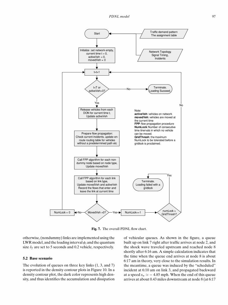
4.4 A flowchart of PDNL

Figure 7 presents an overall PDNL flowchart, which as-sumes the network is empty at the onset. The procedureis terminated either when the network clears out (all re-leased vehicles have arrived at their destinations) or agridlock is detected (no vehicle can be moved becausethey are trapped in an interlock situation). However,other termination criteria may also be considered.

In each time step t, the first operation is to release newquanta from DON based on the time-dependent traveldemand pattern (see Algorithm FPP-DON). Then a pre-process is followed. Incidents, for example, can be takeninto account at this step. In case some vehicles do nothave an assigned path and thereby need route guidance,this preprocess may also include the calculation of in-stantaneous shortest paths.

The main course of PDNL is sequentially processingnodes and links to propagate vehicular quanta. When-ever a link FPP is called, the cumulative traffic counts upto t are recorded. Further, all quanta entering the ENBof a DDL at t will be labeled as “arrived” and therebyremoved from the network.

5 NUMERICAL EXPERIMENTS

5.1 Experiment settings

Consider a network shown in Figure 8, which has eightnodes, seven links, and two O-D pairs. The road prop-erties of the four nondummy links are given in Table 3.The flow-density relationship on all links is assumed tofollow the triangle fundamental diagram illustrated inFigure 9.

The assignment horizon is from 6:00 to 6:30 am, dur-ing which the uniform departure rates for O-D pair 5–6and 5–7 are 1,800 vph, and 2,400 vph, respectively. Anincident occurs on link 3 (see Figure 8) at 6:10 am andthe last 15 minutes during which the capacity is reducedto 25% of its regular value.

Obviously, node 2 is a permanent bottleneck (witha capacity 1,200 vph) because of the downstream lanedrop. The incident will cause a temporal bottleneck(with a capacity 1,200 vph) on link 3. Queues are ex-pected to develop at both locations because the uni-form demands (1,800 and 2,400 vph, respectively) exceedthe capacities of the two bottlenecks. Unless specified

PDNL model 97

Start Traffic demand pattern The assignment table

Network Topology, Signal Timing,

Incidents

Initialize : set network empty, current time t = 0,

activeVeh = 0,movedVeh = 0

Release vehicles from each DON for current time t,

Update activeVeh

t<T or activeVeh>0?

Yes

Terminate. Loading Succeed.

No

Prepare flow propagation:Check current incidents, update en-

route routing table for vehicles without a predetermined path etc

Call FPP algorithm for each non-dummy node based on node type,

Update movedVeh

Call FPP algorithm for each link based on link type,

Update movedVeh and activeVehRecord the flows that enter and

leave the link at current time

MovedVeh =0? NumLock+=1Yes numLock > GridThresh?

Yes

Terminate.Loading failed with a

gridlock

NumLock = 0 No

No

Note:activeVeh: vehicles on networkmovedVeh: vehicles are moved at the current timeFPP: flow propagation procedureNumLock: Number of consecutive time itnervals in which no vehicle can be moved.GridThresh: the maximum NumLock to be tolerated before a gridlock is proclaimed.

t=t+1

Fig. 7. The overall PDNL flow chart.

otherwise, (nondummy) links are implemented using theLWR model, and the loading interval φi and the quantumsize δf are set to 5 seconds and 0.2 vehicle, respectively.

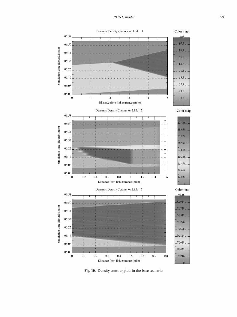
5.2 Base scenario

The evolution of queues on three key links (1, 3, and 7)is reported in the density contour plots in Figure 10. In adensity contour plot, the dark color represents high den-sity, and thus identifies the accumulation and dissipation

of vehicular queues. As shown in the figure, a queuebuilt up on link 7 right after traffic arrives at node 2, andthe shock wave traveled upstream and reached node 8shortly after 6:16 am. A simple calculation indicates thatthe time when the queue end arrives at node 8 is about6:17 am in theory, very close to the simulation results. Inthe meantime, a queue was induced by the “scheduled”incident at 6:10 am on link 3, and propagated backwardat a speed sw � − 4.85 mph. When the end of this queuearrives at about 0.43 miles downstream at node 8 (at 6:17

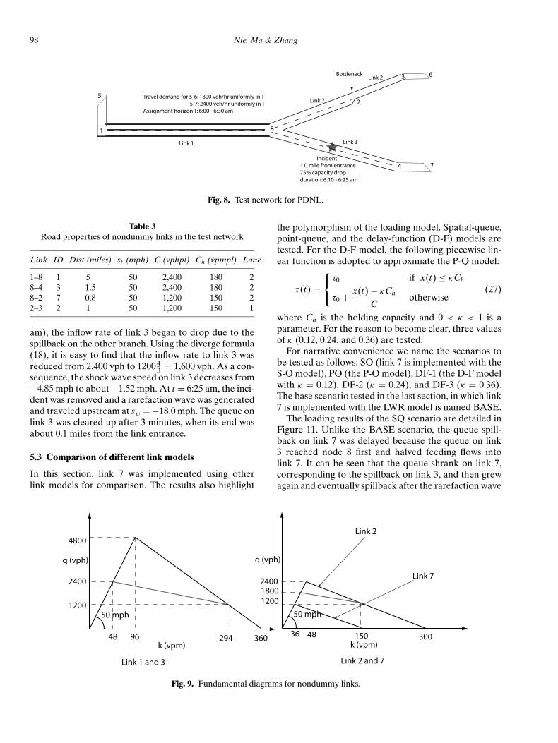
98 Nie, Ma & Zhang

Incident

Bottleneck

Travel demand for 5-6: 1800 veh/hr uniformly in T 5-7: 2400 veh/hr uniformly in T Assignment horizon T: 6:00 - 6:30 am

1.0 mile from entrance75% capacity dropduration: 6:10 - 6:25 am

Link 1 Link 3

Link 7

Link 2 6

1

5

3

2

8

4 7

Fig. 8. Test network for PDNL.

Table 3Road properties of nondummy links in the test network

Link ID Dist (miles) sf (mph) C (vphpl) Ch (vpmpl) Lane

1–8 1 5 50 2,400 180 28–4 3 1.5 50 2,400 180 28–2 7 0.8 50 1,200 150 22–3 2 1 50 1,200 150 1

am), the inflow rate of link 3 began to drop due to thespillback on the other branch. Using the diverge formula(18), it is easy to find that the inflow rate to link 3 wasreduced from 2,400 vph to 1200 4

3 = 1,600 vph. As a con-sequence, the shock wave speed on link 3 decreases from−4.85 mph to about −1.52 mph. At t = 6:25 am, the inci-dent was removed and a rarefaction wave was generatedand traveled upstream at sw = −18.0 mph. The queue onlink 3 was cleared up after 3 minutes, when its end wasabout 0.1 miles from the link entrance.

5.3 Comparison of different link models

In this section, link 7 was implemented using otherlink models for comparison. The results also highlight

4800

q (vph)

k (vpm)36096

50 mph

Link 1 and 3

2400

q (vph)

k (vpm)30048

50 mph

Link 2 and 7

2400

1200

18001200

29448 15036

Link 2

Link 7

Fig. 9. Fundamental diagrams for nondummy links.

the polymorphism of the loading model. Spatial-queue,point-queue, and the delay-function (D-F) models aretested. For the D-F model, the following piecewise lin-ear function is adopted to approximate the P-Q model:

τ (t) =

τ0 if x(t) ≤ κCh

τ0 + x(t) − κCh

Cotherwise

(27)

where Ch is the holding capacity and 0 < κ < 1 is aparameter. For the reason to become clear, three valuesof κ (0.12, 0.24, and 0.36) are tested.

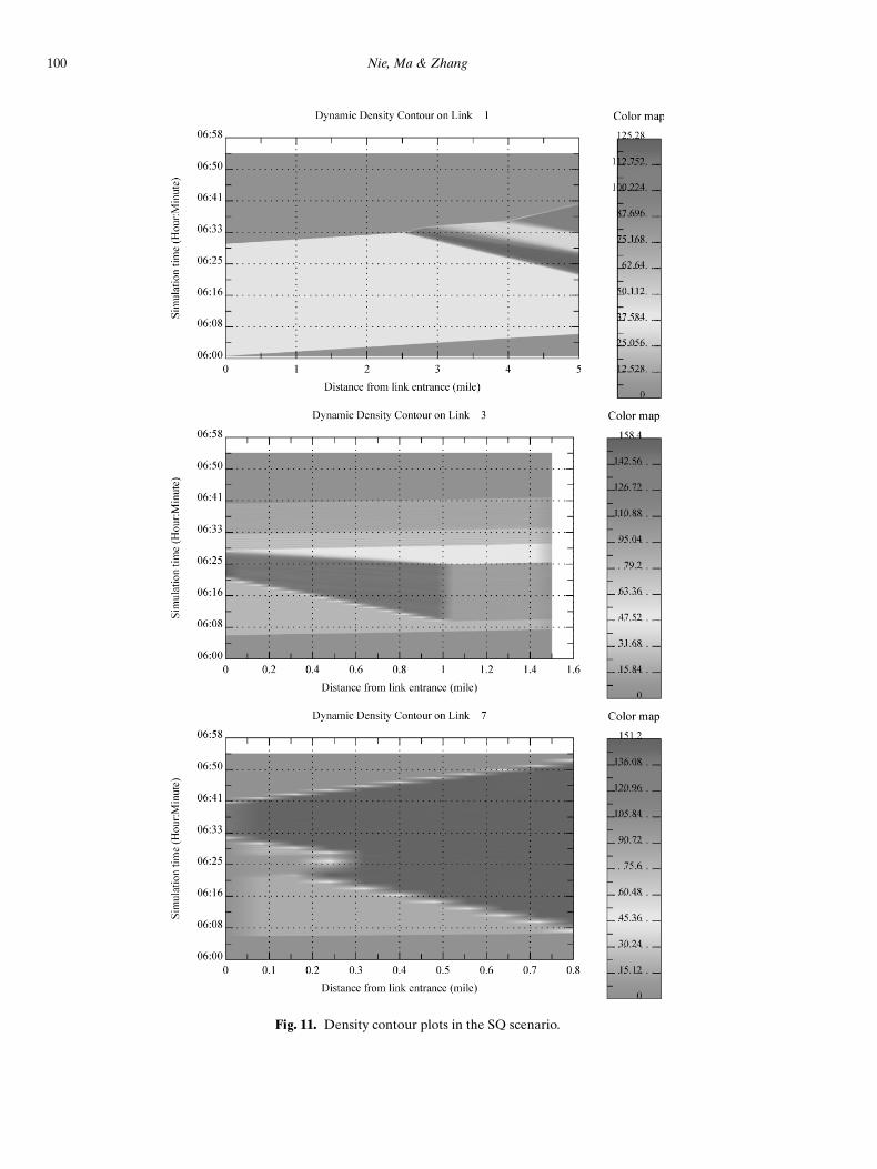
For narrative convenience we name the scenarios tobe tested as follows: SQ (link 7 is implemented with theS-Q model), PQ (the P-Q model), DF-1 (the D-F modelwith κ = 0.12), DF-2 (κ = 0.24), and DF-3 (κ = 0.36).The base scenario tested in the last section, in which link7 is implemented with the LWR model is named BASE.

The loading results of the SQ scenario are detailed inFigure 11. Unlike the BASE scenario, the queue spill-back on link 7 was delayed because the queue on link3 reached node 8 first and halved feeding flows intolink 7. It can be seen that the queue shrank on link 7,corresponding to the spillback on link 3, and then grewagain and eventually spillback after the rarefaction wave

PDNL model 99

Fig. 10. Density contour plots in the base scenario.

100 Nie, Ma & Zhang

Fig. 11. Density contour plots in the SQ scenario.

PDNL model 101

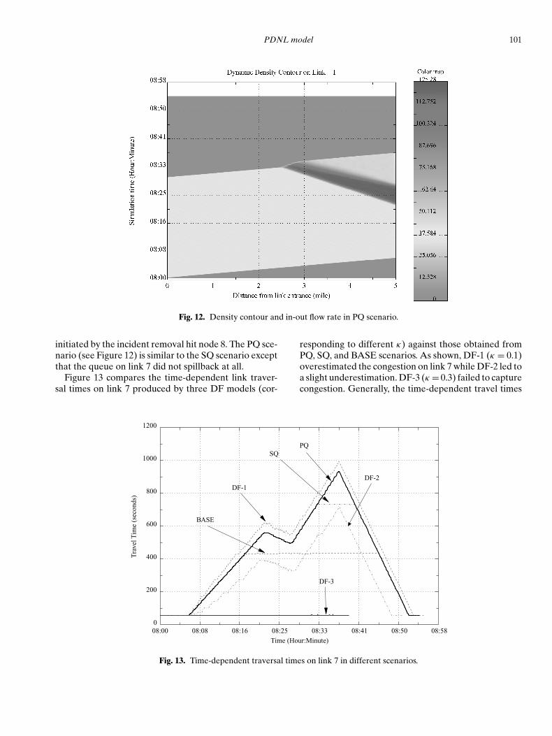
Fig. 12. Density contour and in-out flow rate in PQ scenario.

initiated by the incident removal hit node 8. The PQ sce-nario (see Figure 12) is similar to the SQ scenario exceptthat the queue on link 7 did not spillback at all.

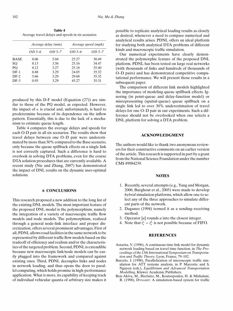
Figure 13 compares the time-dependent link traver-sal times on link 7 produced by three DF models (cor-

DF-3

DF-1

SQ

BASE

DF-2

PQ

08:00 08:08 08:16 08:25 08:33 08:41 08:50 08:580

200

400

600

800

1000

1200

Time (Hour:Minute)

Tra

vel T

ime

(sec

onds

)

Fig. 13. Time-dependent traversal times on link 7 in different scenarios.

responding to different κ) against those obtained fromPQ, SQ, and BASE scenarios. As shown, DF-1 (κ = 0.1)overestimated the congestion on link 7 while DF-2 led toa slight underestimation. DF-3 (κ = 0.3) failed to capturecongestion. Generally, the time-dependent travel times

102 Nie, Ma & Zhang

Table 4Average travel delays and speeds in six scenarios

Average delay (min) Average speed (mph)

OD 5–6 OD 5–7 OD 5–6 OD 5–7

BASE 8.06 5.04 25.27 30.49SQ 8.13 3.56 25.16 34.47PQ 8.12 3.27 25.18 35.40DF-1 8.88 3.29 24.05 35.32DF-2 5.66 3.29 29.68 35.32DF-3 0.93 3.29 45.27 35.31

produced by this D-F model (Equation (27)) are sim-ilar to those of the PQ model, as expected. However,the impact of κ is crucial and, unfortunately, is hard topredetermine because of its dependence on the inflowpattern. Essentially, this is due to the lack of a mecha-nism to estimate queue length.

Table 4 compares the average delays and speeds foreach O-D pair in all six scenarios. The results show thattravel delays between one O–D pair were underesti-mated by more than 30% compared to the Base scenario,only because the queue spillback effects on a single linkis not correctly captured. Such a difference is hard tooverlook in solving DTA problems, even for the coarseDTA solution procedures that are currently available. Arecent study (Nie and Zhang, 2007) has demonstratedthe impact of DNL results on the dynamic user-optimalsolutions.

6 CONCLUSIONS

This research proposed a new addition to the long list ofthe existing DNL models. The most important feature ofthe proposed DNL model is the polymorphism, namelythe integration of a variety of macroscopic traffic flowmodels and node models. The polymorphism, realizedthrough a general node-link interface and proper dis-cretization, offers several prominent advantages. First ofall, PDNL allows road facilities in the same network to berepresented by different traffic flow models based on thetradeoff of efficiency and realism and/or the characteris-tics of the targeted problem. Second, PDNL is extendiblebecause new macroscopic link/node models can be eas-ily plugged into the framework and compared againstexisting ones. Third, PDNL decouples links and nodesin network loading, and thus opens the door to paral-lel computing, which holds promise in high-performanceapplication. What is more, its capability of keeping trackof individual vehicular quanta of arbitrary size makes it

possible to replicate analytical loading results as closelyas desired, whenever a need to compare numerical andanalytical results arises. PDNL offers an ideal platformfor studying both analytical DTA problems of differentkinds and macroscopic traffic simulation.

Our numerical experiments have clearly demon-strated the polymorphic feature of the proposed DNLplatform. PDNL has been tested on large real networks(with thousands of links and hundreds of thousands ofO–D pairs) and has demonstrated competitive compu-tational performance. We will present those results in asubsequent paper.

The comparison of different link models highlightedthe importance of modeling queue spillback effects. Ig-noring (in point-queue and delay-function model) ormisrepresenting (spatial-queue) queue spillback on asingle link led to over 30% underestimation of traveldelays for one O–D pair in our experiments. Such a dif-ference should not be overlooked when one selects aDNL platform for solving a DTA problem.

ACKNOWLEDGMENT

The authors would like to thank two anonymous review-ers for their constructive comments on an earlier versionof the article. This research is supported in part by a grantfrom the National Science Foundation under the numberCMS #9984239.

NOTES

1. Recently, several attempts (e.g., Yang and Morgan,2006; Burghout et al., 2005) were made to develophybrid simulation platforms, which allow one to se-lect any of the three approaches to simulate differ-ent parts of the network.

2. Daganzo (1994) termed it as a sending–receivingmethod.

3. Operator [a] rounds a into the closest integer.4. Note that t∗e < tLe is not possible because of FIFO.

REFERENCES

Astarita, V. (1996), A continuous time link model for dynamicnetwork loading based on travel time function, in The Pro-ceedings of the 13th International Symposium on Transporta-tion and Traffic Theory, Lyon, France, 79–102.

Barcelo, J. (1998), Parallelization of microscopic traffic sim-ulation for ATT systems analysis, in P. Marcotte and S.Nguyen (eds.), Equilibrium and Advanced TransportationModelling, Kluwer Academic Publishers.

Ben-Akiva, M., Bierlaire, M., Koutsopoulos, H. & Mishalani,R. (1998), DYNAMIT: A simulation-based system for traffic

PDNL model 103

prediction, presented at the DAC-CORD short-term fore-casting workshop, Delft, The Netherlands.

Burghout, W., Koutsopoulos, H. N. & Andreasson, I. (2005),Hybrid mesoscopic-microscopic traffic simulation, Trans-portation Research Record, 1934, 218–225.

Bush, B. W. (2000), An Algorithmic Overview of TRANSIMS,Los Alamos National Laboratories.

Carey, M. & Ge, Y. E. (2005), Convergence of a discretisedtravel-time model, Transportation Science, 39, 25–38.

Carey, M. & McCartney, M. (2002), Behaviour of a whole-link travel time model used in dynamic traffic assignment,Transportation Research, 36B, 83–95.

Courant, R., Friedrichs, K. & Lewy, H. (1928), ber die par-tiellen differenzengleichungen der-mathematischen physik,Mathematische Annalen, 100, 32–74.

Daganzo, C. F. (1994), The cell transmission model: A dy-namic representation of highway traffic consistent with thehydrodynamic theory, Transportation Research, 28B, 269–287.

Daganzo, C. F. (1995a), The cell transmission model, part II:Network traffic, Transportation Research, 29B, 79–93.

Daganzo, C. F. (1995b), Properties of link travel times underdynamic load, Transportation Research, 29B, 95–98.

Daganzo, C. F. (2005a), A variational formulation of kine-matic waves: Basic theory and complex boundary conditions,Transportation Research, 39B, 187–96.

Daganzo, C. F. (2005b), A variational formulation of kine-matic waves: Solution methods, Transportation Research,39B, 934–50.

Fellendorf, M. (1994), VISSIM: A microscopic simulation toolto evaluate actuated signal control including bus priority,presented at the 64th ITE Annual Meeting, Session 32, Dal-las.

Friesz, T. L., Bernstein, D., Smith, T. E., Tobin, R. L. & Wei,B. W. (1993), A variational inequality formulation of thedynamic network equilibrium problem, Operation Research,41, 179–91.

FWHA, (1996), CORSIM User Guide. Technical ReportVersion 1.0, Federal Highway Administration, US-DOT,McLean, Virginia.

Godunov, S. K. (1959), A difference method for numerical cal-culations of discontinuous solutions of the equations of hy-drodynamics, Matematicheskii Sbornik, in Russian, 47, 271–306.

Jin, W.-L. (2003), Kinematic wave traffic flow models for roadnetworks: Theories, simulations, and applications, PhD the-sis, The University of California, Davis, CA.

Jin, W.-L. & Zhang, H. M. (2001), On the distribution schemesin the discrete kinematic wave model of merges, Transporta-tion Research, 37B, 521–40.

Jin, W.-L. & Zhang, H. M. (2004), A multicommodity kine-matic wave simulation model of network traffic flow, Trans-portation Research Record 1883, 59–67.

Lebacque, J. P. (1996), The Godunov scheme and what it meansfor firrst order traffic flow models, in Proceedings of the 13thInternational Symposium on Transportation and Traffic The-ory, Lyon, France, 647–677.

Lebacque, J. P. & Khoshyaran, M. M. (2005), First order macro-scopic traffic flow models: intersections modeling, networkmodeling, in H. S. Mahmassani (ed.), Proceedings of the 16thInternational Symposium of Transportation and Traffic The-ory, College Park, MD, pp. 365–86.

Lighthill, M. J. & Whitham, J. B. (1955), On kinematic waves.I. flow modeling in long rivers. II. a theory of traffic flowon long crowded roads, Proceedings of the Royal Society A,229, 291–345.

Luke, J. (1972), Mathematical models for landform evolution,Journal of Geophysical Research, 77, 2460–4.

Mahmassani, H. S. (2000), DYNASMART-P, volume II, userguide, Technical Report STO67-85-PII, Center for Trans-portation Research, The University of Texas at Austin.

Mahut, M., Florian, M. & Tremblay, N. (2003), Space-timequeues and dynamic traffic assignment: A model, algorithmand applications, presented at the 82th Annual Meeting ofTransportation Research Board, Washington DC.

Merchant, D. K. & Nemhauser, G. L. (1978a), A model andan algorithm for the dynamic traffic assignment problem,Transportation Science, 12, 183–99.

Merchant, D. K. & Nemhauser, G. L. (1978b), Optimality con-ditions for a dynamic traffic assignment model, Transporta-tion Science, 12, 200–7.

Michalopoulos, P., Beskos, D. & Lin, J. (1984), Analysis of in-terrupted traffic flow by finite difference methods, Trans-portation Research, 18B, 409–21.

Michalopoulos, P. & Plum, R. (1986), KRONOS-4: Final Re-port and Users Manual, Minnesota Department of Trans-portation.

Newell, G. F. (1993), A simplified theory of kinematic waves inhighway traffic, Transportation Research, 27B, 281–314.

Nie, Y. (2006), A Variational Inequality Approach ForInferring Dynamic Origin-Destination Travel Demands,PhD thesis, The University of California, Davis, CA,http://www.civil.northwestern.edu/people/nie/nie-diss.pdf.

Nie, Y. & Zhang, H. M. (2007), Solving the dynamic useroptimal assignment problem considering queue spillback,Networks and Spatial Economics, available at http://www.springerlink.com/content/w6653261h1uOr57/.

Palma, A. D. & Marchal, F. (1998), Analysis of traffic costcomponents using large-scale, dynamic traffic models, Trans-portation Research Record, 1676, 177–83.

Papageorgiou, M. (1990), Dynamic modeling, assignment, androute guidance in traffic net-works, Transportation Research,24B, 471–95.

Payne, H. J. (1979), FREFLO: A macroscopic simulationmodel of freeway traffic, Transporta-tion Research Record,722, 68–77.

Quadstone (2002), PARAMICS user guide and references, Tech-nical report.

Richards, P. I. (1956), Shockwaves on the highway, OperationResearch, 4, 42–51.

Taylor, N. B. (1990), CONTRAM 5: An enhanced trac assign-ment model, Report RR249, Transport and Research Lab-oratory, Crowthorne, UK.

Van-Aerde, M. & Yagar, S. (1988), Dynamic integrated free-way/traffic signal networks: A routing-based modelling ap-proach, Transportation Research, 22A, 445–53.

Velan, S. M. (2000), The cell-transmission model: A new lookat a dynamic network loading model, PhD thesis, Center forresearch on transportation, University of Montreal, Canada.

Xu, Y. W.,Wu, J. H., Florian, M., Marcotte, P. & Zhu, D. L.(1999), Advances in the continuous dynamic network load-ing problem, Transportation Science, 33, 341–53.

Yang, Q. & Koutsopoulos, H. N. (1996), A microscopic traf-fic simulator for evaluation of dynamic traffic managementsystems, Transportation Research, 4C(3), 113–29.

Yang, Q. & Morgan, D. (2006), A hybrid traffic simulationmodel, presented at 85th Annual Meeting of TransportationResearch Board, Washington DC.

Zhang, H. M. & Nie, Y. (2006), Modeling network flow withand without link interaction: properties and implications,presented at the 84th annual meeting of the TransportationResearch Board, Washington DC.