A Physics-Based Emissions Model for Aircraft Gas Turbine Combustors by Douglas L. Allaire Submitted to the Department of Aeronautics and Astronautics in partial fulfillment of the requirements for the degree of Master of Science in Aerospace Engineering at the MASSACHUSETTS INSTITUTE OF TECHNOLOGY May 2006 c Massachusetts Institute of Technology 2006. All rights reserved. Author .............................................................. Department of Aeronautics and Astronautics May 26, 2006 Certified by .......................................................... Karen Willcox Associate Professor Thesis Supervisor Certified by .......................................................... Ian Waitz Professor Thesis Supervisor Accepted by ......................................................... Jaime Peraire Professor of Aeronautics and Astronautics Chairman, Department Committee on Graduate Students

A Physics-Based Emissions Model for Aircraft Gas Turbine ...
Dec 25, 2015
Aircraft Gas turbine Emissions
Welcome message from author
This document is posted to help you gain knowledge. Please leave a comment to let me know what you think about it! Share it to your friends and learn new things together.
Transcript

A Physics-Based Emissions Model for Aircraft Gas
Turbine Combustors
by
Douglas L. Allaire
Submitted to the Department of Aeronautics and Astronautics
in partial fulfillment of the requirements for the degree of
Master of Science in Aerospace Engineering
at the
MASSACHUSETTS INSTITUTE OF TECHNOLOGY
May 2006
c© Massachusetts Institute of Technology 2006. All rights reserved.
Author . . . . . . . . . . . . . . . . . . . . . . . . . . . . . . . . . . . . . . . . . . . . . . . . . . . . . . . . . . . . . .Department of Aeronautics and Astronautics
May 26, 2006
Certified by. . . . . . . . . . . . . . . . . . . . . . . . . . . . . . . . . . . . . . . . . . . . . . . . . . . . . . . . . .Karen Willcox
Associate Professor
Thesis Supervisor
Certified by. . . . . . . . . . . . . . . . . . . . . . . . . . . . . . . . . . . . . . . . . . . . . . . . . . . . . . . . . .
Ian WaitzProfessor
Thesis Supervisor
Accepted by . . . . . . . . . . . . . . . . . . . . . . . . . . . . . . . . . . . . . . . . . . . . . . . . . . . . . . . . .Jaime Peraire
Professor of Aeronautics and AstronauticsChairman, Department Committee on Graduate Students

2

A Physics-Based Emissions Model for Aircraft Gas Turbine
Combustors
by
Douglas L. Allaire
Submitted to the Department of Aeronautics and Astronauticson May 26, 2006, in partial fulfillment of the
requirements for the degree ofMaster of Science in Aerospace Engineering
Abstract
In this thesis, a physics-based model of an aircraft gas turbine combustor is developedfor predicting NOx and CO emissions. The objective of the model is to predict theemissions of current and potential future gas turbine engines within quantified uncer-tainty bounds for the purpose of assessing design tradeoffs and interdependencies ina policy-making setting. The approach taken is to capture the physical relationshipsamong operating conditions, combustor design parameters, and pollutant emissions.The model is developed using only high-level combustor design parameters and idealreactors. The predictive capability of the model is assessed by comparing modelestimates of NOx and CO emissions from five different industry combustors to certi-fication data.
The model developed in this work correctly captures the physical relationshipsbetween engine operating conditions, combustor design parameters, and NOx andCO emissions. The NOx estimates are as good as, or better than, the NOx estimatesfrom an established empirical model; and the CO estimates are within the uncertaintyin the certification data at most of the important low power operating conditions.
Thesis Supervisor: Karen WillcoxTitle: Associate Professor
Thesis Supervisor: Ian WaitzTitle: Professor
3

4

Acknowledgments
The work presented in this thesis was possible because of the technical support pro-
vided by a number of people. To all of these people I owe a great deal of thanks. First
and foremost, I would like to thank my advisors, Prof. Karen Willcox and Prof. Ian
Waitz. Their assistance and guidance in the technical aspects of this work was crucial
to its completion. I would also like to thank Joe Palladino, who provided me with
expert knowledge of the aircraft engine industry and every bit of data that I thought
could help with the research. I also received a great deal of help from industry that
made this research possible. For this I would like to thank Frank Lastrina and Hukam
Mongia from General Electric and Nan-Suey Liu from NASA Glenn. A great deal
of thanks is also owed to Sean Bradshaw and Steve Lukachko for handling all of the
questions I asked them along the way with patience and a genuine interest in helping
me get a handle on combustion and to Garrett Barter, who guided me through several
computer related issues that would have taken me weeks to figure out on my own.
Finally, I would like to thank my friends and my family for their support during
this research and throughout my life.
5

6

Contents
1 Introduction 15
1.1 Motivation for Emissions Prediction . . . . . . . . . . . . . . . . . . . 15
1.1.1 Major Aircraft Engine Emissions . . . . . . . . . . . . . . . . 16
1.1.2 The ICAO Regulation Process . . . . . . . . . . . . . . . . . . 18
1.1.3 An Emissions Tool for Trade Studies . . . . . . . . . . . . . . 19
1.2 Necesssary Attributes of an Emissions Model for Policy Making . . . 21
1.3 Current Emissions Prediction Strategies and Techniques . . . . . . . 21
1.3.1 Empirical Models . . . . . . . . . . . . . . . . . . . . . . . . . 21
1.3.2 Semiempirical Models . . . . . . . . . . . . . . . . . . . . . . 24
1.3.3 Simplified Physics-Based Models . . . . . . . . . . . . . . . . 25
1.3.4 High Fidelity Simulations . . . . . . . . . . . . . . . . . . . . 25
1.3.5 State of the Art for Emissions Trade Analyses . . . . . . . . . 26
1.4 A Physics-Based Emissions Model . . . . . . . . . . . . . . . . . . . . 27
1.4.1 Objective . . . . . . . . . . . . . . . . . . . . . . . . . . . . . 27
1.4.2 Emissions Model Success Criteria . . . . . . . . . . . . . . . . 27
1.5 Thesis Outline . . . . . . . . . . . . . . . . . . . . . . . . . . . . . . . 28
2 Developing a Physics-Based Emissions Model 29
2.1 Functional Requirements . . . . . . . . . . . . . . . . . . . . . . . . . 29
2.2 Model Input/Output . . . . . . . . . . . . . . . . . . . . . . . . . . . 30
2.3 Combustion Fundamentals . . . . . . . . . . . . . . . . . . . . . . . . 30
2.4 Governing Equations . . . . . . . . . . . . . . . . . . . . . . . . . . . 31
2.5 Reducing the Governing Equations . . . . . . . . . . . . . . . . . . . 32
7

2.5.1 The Perfectly Stirred Reactor . . . . . . . . . . . . . . . . . . 32
2.5.2 PLUG Flow Reactor . . . . . . . . . . . . . . . . . . . . . . . 35
2.6 Modeling a Gas Turbine Combustor with Ideal Reactors . . . . . . . 36
2.6.1 The Role of the Primary Zone . . . . . . . . . . . . . . . . . . 36
2.6.2 Modeling the Primary Zone . . . . . . . . . . . . . . . . . . . 37
2.6.3 Primary Zone Emissions Considerations . . . . . . . . . . . . 37
2.6.4 Assumptions and Limitations of the Primary Zone Model . . . 41
2.6.5 The Role of the Intermediate Zone . . . . . . . . . . . . . . . 42
2.6.6 Modeling the Intermediate Zone . . . . . . . . . . . . . . . . . 42
2.6.7 Intermediate Zone Emissions Considerations . . . . . . . . . . 44
2.6.8 Assumptions and Limitations of the Intermediate Zone Models 44
2.6.9 The Role of the Dilution Zone . . . . . . . . . . . . . . . . . . 44
2.6.10 Modeling the Dilution Zone . . . . . . . . . . . . . . . . . . . 44
2.6.11 Modeling the Injection of Dilution/Cooling Air . . . . . . . . 45
2.6.12 Assumptions and Limitations of Injection Mapping . . . . . . 46
2.6.13 Model Implementation . . . . . . . . . . . . . . . . . . . . . . 47
2.6.14 The Physics-Based Emissions Model . . . . . . . . . . . . . . 47
3 Setting the Unmixedness Parameter 49
3.1 Industry Data . . . . . . . . . . . . . . . . . . . . . . . . . . . . . . . 50
3.2 Sensitivity to Unmixedness . . . . . . . . . . . . . . . . . . . . . . . . 50
3.2.1 Single Value Optimization . . . . . . . . . . . . . . . . . . . . 50
3.2.2 General Curve Optimization . . . . . . . . . . . . . . . . . . . 52
3.2.3 Individual Curve Optimization . . . . . . . . . . . . . . . . . 54
3.3 Evaluating the Different Options . . . . . . . . . . . . . . . . . . . . 55
3.3.1 Single Point Estimate . . . . . . . . . . . . . . . . . . . . . . . 55
3.3.2 General Curve Estimate . . . . . . . . . . . . . . . . . . . . . 56
3.3.3 Individual Curve Estimate . . . . . . . . . . . . . . . . . . . . 56
3.4 Setting Unmixedness . . . . . . . . . . . . . . . . . . . . . . . . . . . 57
3.5 Unmixedness Parameter Issues . . . . . . . . . . . . . . . . . . . . . . 57
8
4 Assessing the Predictive Capability of the Model 61
4.1 NOx Chemistry . . . . . . . . . . . . . . . . . . . . . . . . . . . . . . 61
4.2 CO Chemistry . . . . . . . . . . . . . . . . . . . . . . . . . . . . . . . 63
4.3 Predicting NOx and CO Chemically . . . . . . . . . . . . . . . . . . . 64
4.4 Model Response to T3 . . . . . . . . . . . . . . . . . . . . . . . . . . 64
4.5 Model Response to P3 . . . . . . . . . . . . . . . . . . . . . . . . . . 66
4.6 Model Response to Equivalence Ratio . . . . . . . . . . . . . . . . . . 68
4.7 Capturing the Effects of Gas Turbine Combustor Design . . . . . . . 70
4.7.1 Idle Emissions Output . . . . . . . . . . . . . . . . . . . . . . 70
4.7.2 Approach Emissions Output . . . . . . . . . . . . . . . . . . . 71
4.7.3 Climb-Out Emissions Output . . . . . . . . . . . . . . . . . . 73
4.7.4 Takeoff Emissions Output . . . . . . . . . . . . . . . . . . . . 73
4.7.5 Assessment of Model Capability . . . . . . . . . . . . . . . . . 75
5 Results 77
5.1 Model Predictions for Engines 1, 2, and 3 . . . . . . . . . . . . . . . . 77
5.1.1 Overview of the Results . . . . . . . . . . . . . . . . . . . . . 78
5.1.2 Engine 1 Estimates . . . . . . . . . . . . . . . . . . . . . . . . 78
5.1.3 Engine 2 Estimates . . . . . . . . . . . . . . . . . . . . . . . . 80
5.1.4 Engine 3 Estimates . . . . . . . . . . . . . . . . . . . . . . . . 80
5.1.5 Overall Estimates . . . . . . . . . . . . . . . . . . . . . . . . . 83
5.1.6 Discussion of Engine 1, 2, and 3 Model Estimates . . . . . . . 84
5.2 Predicting the Effects of Design Changes . . . . . . . . . . . . . . . . 84
5.2.1 Overview of Results . . . . . . . . . . . . . . . . . . . . . . . . 84
5.2.2 Engine 1a to Engine 1 . . . . . . . . . . . . . . . . . . . . . . 85
5.2.3 Discussion of the Engine 1a to Engine 1 Design Change Results 88
5.2.4 Engine 3 to Engine 3a . . . . . . . . . . . . . . . . . . . . . . 89
5.2.5 Discussion of the Engine 3 to Engine 3a Design Change Results 92
5.3 NOx Estimates for a Full Throttle Sweep . . . . . . . . . . . . . . . . 93
5.3.1 Throttle Sweep Emissions Estimates . . . . . . . . . . . . . . 93
9

5.3.2 Throttle Sweep Estimates versus Boeing Fuel Flow Method 2 . 94
6 Conclusions and Future Work 97
6.1 Conclusions . . . . . . . . . . . . . . . . . . . . . . . . . . . . . . . . 97
6.2 Future Work . . . . . . . . . . . . . . . . . . . . . . . . . . . . . . . . 100
10

List of Figures
1-1 Regional NOx Emissions in the US [7] . . . . . . . . . . . . . . . . . . 17
1-2 Radiative Forcing from Aircraft [9] . . . . . . . . . . . . . . . . . . . 18
1-3 ICAO LTO Cycle [8] . . . . . . . . . . . . . . . . . . . . . . . . . . . 19
1-4 NOx Emissions by Combustor Technology Generation [10] . . . . . . 20
2-1 Diagram of a Perfectly Stirred Reactor, adapted from [17] . . . . . . 33
2-2 Diagram of a Plug Flow Reactor, adapted from [17] . . . . . . . . . . 35
2-3 The Effect of Turbulence on Damkohler Number [18] . . . . . . . . . 38
2-4 Normal Distribution of Equivalence Ratio in the Primary Zone PSRs 39
2-5 Determining the Primary Zone Model . . . . . . . . . . . . . . . . . . 40
2-6 Diagram of the Primary Zone Model . . . . . . . . . . . . . . . . . . 41
2-7 Diagram of the Intermediate Zone Model . . . . . . . . . . . . . . . . 43
2-8 Diagram of the Dilution Zone Model . . . . . . . . . . . . . . . . . . 45
2-9 Typical Combustor Flow Splits . . . . . . . . . . . . . . . . . . . . . 46
2-10 Diagram of the Physics-Based Emissions Model . . . . . . . . . . . . 47
3-1 Response of Engine 1a Emissions to Varying Unmixedness . . . . . . 51
3-2 Unmixedness versus Primary Zone Equivalence Ratio [19] . . . . . . . 53
3-3 Model Unmixedness versus Primary Zone Equivalence Ratio . . . . . 54
3-4 Model Unmixedness versus Primary Zone Equivalence Ratio for LTO
Cycle . . . . . . . . . . . . . . . . . . . . . . . . . . . . . . . . . . . . 55
4-1 Model EINOx versus Combustor Inlet Temperature . . . . . . . . . . 65
4-2 Model EICO versus Combustor Inlet Temperature . . . . . . . . . . . 66
11

4-3 Effect of Pressure on Flame Temperature, adapted from [14] . . . . . 67
4-4 Model EINOx versus Combustor Inlet Pressure . . . . . . . . . . . . . 67
4-5 Model EICO versus Combustor Inlet Pressure . . . . . . . . . . . . . 68
4-6 Model EINOx versus Primary Zone Equivalence Ratio . . . . . . . . . 69
4-7 Model EICO versus Primary Zone Equivalence Ratio . . . . . . . . . 70
4-8 Model Combustor Zone Emissions Production at Idle Power . . . . . 71
4-9 Model Combustor Zone Emissions Production at Approach Power . . 72
4-10 Carbon Monoxide Emissions versus Primary Zone Equivalence Ratio
[14] . . . . . . . . . . . . . . . . . . . . . . . . . . . . . . . . . . . . . 73
4-11 Model Combustor Zone Emissions Production at Climb Out Power . 74
4-12 Model Combustor Zone Emissions Production at Takeoff Power . . . 74
5-1 Emissions Estimates for Engine 1 . . . . . . . . . . . . . . . . . . . . 79
5-2 Emissions Estimates for Engine 2 . . . . . . . . . . . . . . . . . . . . 81
5-3 Emissions Estimates for Engine 3 . . . . . . . . . . . . . . . . . . . . 82
5-4 Emissions Estimates for Engines 1, 2, and 3 . . . . . . . . . . . . . . 83
5-5 Percentage Change of Inputs from Engine 1 to Engine 1a . . . . . . . 89
5-6 Percentage Change of Inputs from Engine 3 to Engine 3a . . . . . . . 92
5-7 Throttle Sweep Emissions Estimates for Engine 1a . . . . . . . . . . . 94
5-8 Throttle Sweep Emissions Estimates for Engine 1a Compared with
Boeing Fuel Flow Method 2 . . . . . . . . . . . . . . . . . . . . . . . 95
12

List of Tables
1.1 Full Simulation Time [15] . . . . . . . . . . . . . . . . . . . . . . . . 26
3.1 Relative Power of Each Engine in the Study . . . . . . . . . . . . . . 50
3.2 Single Value Optimized Unmixedness . . . . . . . . . . . . . . . . . . 52
3.3 Comparison of Engine 1 Calculated and Optimized Unmixedness . . . 56
3.4 Comparison of Engine 1a Calculated and Optimized Unmixedness . . 56
3.5 Comparison of Engine 1a Calculated and Optimized Unmixedness . . 57
3.6 Comparison of Engine 1a Calculated and Optimized Unmixedness . . 59
5.1 Engine 1a NOx Emissions . . . . . . . . . . . . . . . . . . . . . . . . 85
5.2 Engine 1a CO Emissions . . . . . . . . . . . . . . . . . . . . . . . . . 86
5.3 Engine 1 NOx Emissions . . . . . . . . . . . . . . . . . . . . . . . . . 86
5.4 Engine 1a and Engine 1 NOx Dp/Foo Estimates . . . . . . . . . . . . 87
5.5 Engine 1 CO Emissions . . . . . . . . . . . . . . . . . . . . . . . . . . 87
5.6 Engine 1a and Engine 1 CO Dp/Foo Estimates . . . . . . . . . . . . 88
5.7 Engine 3 NOx Emissions . . . . . . . . . . . . . . . . . . . . . . . . . 90
5.8 Engine 3 CO Emissions . . . . . . . . . . . . . . . . . . . . . . . . . . 90
5.9 Engine 3a NOx Emissions . . . . . . . . . . . . . . . . . . . . . . . . 91
5.10 Engine 3 and Engine 3a NOx Dp/Foo Estimates . . . . . . . . . . . . 91
5.11 Engine 3a CO Emissions . . . . . . . . . . . . . . . . . . . . . . . . . 91
5.12 Engine 3 and Engine 3a CO Dp/Foo Estimates . . . . . . . . . . . . 92
13

14
Chapter 1
Introduction
Increasing concern over local air quality, community noise, and climate change caused
by air transportation has led to an effort aimed at developing a means to articulate
trade-offs at the aircraft design level among fuel burn, emissions of local air quality
pollutants, cruise emissions, and community noise. A tool, called the Environmental
Design Space (EDS), is therefore being created, which is intended as an aircraft
system level design tool for use in regulatory policy making within the FAA and
the International Civil Aviation Organization (ICAO). A critical aspect of EDS is
the development of an emissions model capable of capturing the interdependencies
between different emissions, noise, and engine performance. The development of such
an emissions model is the topic of this thesis.
1.1 Motivation for Emissions Prediction
The worldwide fleet of aircraft is expected to more than double in the next twenty
years [1]. Development of new technology is not expected offset the increase in emis-
sions caused by the growth in aviation [2]. Due to a lag in the introduction of tech-
nology in the aviation industry, the time required to transition from basic research
to fleet impact can be as much as 25 years [3]. Because of this, a method is desired
for assessing the influence of different policy scenarios regarding trade-offs on engine
emissions and other aircraft design parameters.
15
1.1.1 Major Aircraft Engine Emissions
Emissions from aircraft engines that impact local air quality are oxides of nitrogen,
carbon monoxide, soot, unburned hydrocarbons, and oxides of sulfur. Oxides of
nitrogen, commonly referred to as NOx, consist of NO and NO2, and are the most
highly regulated pollutants from aircraft engines [4]. NOx emissions also tend to be
difficult to control because changes in engine design aimed at improving fuel efficiency
often make it more challenging to limit NOx production. Between 1970 and 1998 for
example, emissions of all major aircraft pollutants except for NOx, decreased, while
NOx emissions increased by about 10% [5].
Carbon monoxide, known as CO, is another regulated emission. According to work
done by Lukachko and Waitz however, the impact of aviation CO on the environment
is only about 1/100th of the impact of NOx emissions [6]. Even so, CO emissions are
regulated and need to be accounted for by an emissions prediction model.
While there are other important emissions from aircraft engines, in particular
soot, this thesis focuses only on modeling the gaseous emissions, NOx and CO.
Local NOx Emissions
Both NOx and CO emissions are regulated because of their effects on the environment
and on human health. The effects of CO are mainly local, while the effects of NOx are
felt both locally and globally. As shown in Figure 1-1, in 1999 it was predicted that by
2010 there would be significant increases in regional NOx produced by aircraft relative
to what was being produced in 1990. Worldwide low altitude NOx emissions from
aircraft are expected to increase by a factor of 2.6 between 2002 and 2020 [5]. These
anticipated increases in NOx are of concern because of the health issues associated
with local NOx production, in particular the production of ground-level ozone (smog),
which can lead to respiratory problems and other detriments to human health.
16

Figure 1-1: Regional NOx Emissions in the US [7]
Local CO Emissions
CO has been reduced by operating at nearly 100% combustion efficiency at high power
settings. While taxiing on airport runways, however, combustors do not operate as
efficiently and higher levels of CO are produced. Carbon monoxide emissions caused
by idling aircraft engines in airports are a health concern because CO reduces the
oxygen carrying capacity of blood and significantly reduces the ability of a person to
perform physical activities.
Cruise Emissions
As mentioned previously, NOx emissions also have a global effect. This is because at
cruise altitude, emissions of NOx contribute to the formation of atmospheric ozone
and the depletion of atmospheric methane. Significant NOx emissions injected di-
rectly into the upper troposphere/lower stratosphere, may lead to climate change.
Figure 1-2 shows the estimated contributions to radiative forcing of aircraft emissions
in 1992 as well as a projection to 2050. Radiative forcing essentially means the ap-
proximate global effect on climate and the labels: good, fair, poor, refer to the level
of understanding of the effect. The whiskers on the figures are the 67% confidence
17

Figure 1-2: Radiative Forcing from Aircraft [9]
limits. The 2050 projection has a scale that is about a factor of five different from
the scale in 1992, showing that the effects of aircraft emissions on the global climate
are expected to increase. For this reason policies to control cruise emissions are being
considered and an emissions model should be capable of predicting aircraft engine
emissions at all engine settings.
1.1.2 The ICAO Regulation Process
The International Civil Aviation Organization, (ICAO), determines the emissions
regulations to be met by all subscribing countries. The method the ICAO uses is
based only on the landing-takeoff cycle (LTO cycle). The LTO cycle is shown in
Figure 1-3, where idle is 7% sea level static (SLS) thrust, approach is 30%, climb out
is 85%, and takeoff is 100% SLS thrust. Engines are certified based on time in mode
(TIM), which is defined in Figure 1-3, emissions index (EI), fuel flow rate (mf), and
rated output (RO). An emissions index is defined as the ratio of grams of a particular
pollutant to kilograms of fuel burned. The certification variable for each pollutant is
in the form of a Dp/Foo, which is defined as
Dp/Foo =
4∑
i=1
EIi × TIMi × mfi/RO, (1.1)
18
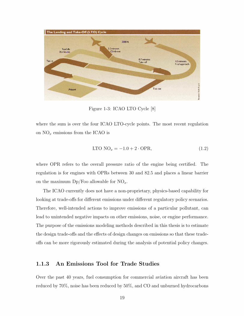
Figure 1-3: ICAO LTO Cycle [8]
where the sum is over the four ICAO LTO-cycle points. The most recent regulation
on NOx emissions from the ICAO is
LTO NOx = −1.0 + 2 · OPR, (1.2)
where OPR refers to the overall pressure ratio of the engine being certified. The
regulation is for engines with OPRs between 30 and 82.5 and places a linear barrier
on the maximum Dp/Foo allowable for NOx.
The ICAO currently does not have a non-proprietary, physics-based capability for
looking at trade-offs for different emissions under different regulatory policy scenarios.
Therefore, well-intended actions to improve emissions of a particular pollutant, can
lead to unintended negative impacts on other emissions, noise, or engine performance.
The purpose of the emissions modeling methods described in this thesis is to estimate
the design trade-offs and the effects of design changes on emissions so that these trade-
offs can be more rigorously estimated during the analysis of potential policy changes.
1.1.3 An Emissions Tool for Trade Studies
Over the past 40 years, fuel consumption for commercial aviation aircraft has been
reduced by 70%, noise has been reduced by 50%, and CO and unburned hydrocarbons
19
(UHC) have been reduced by about 90% [5]. These improvements have come from
the ability to increase OPR, bypass ratio, and turbine entry temperature (TET), due
to better materials and cooling methods, which leads to higher thermal efficiency and
combustion efficiency. During this same time period however, as previously noted,
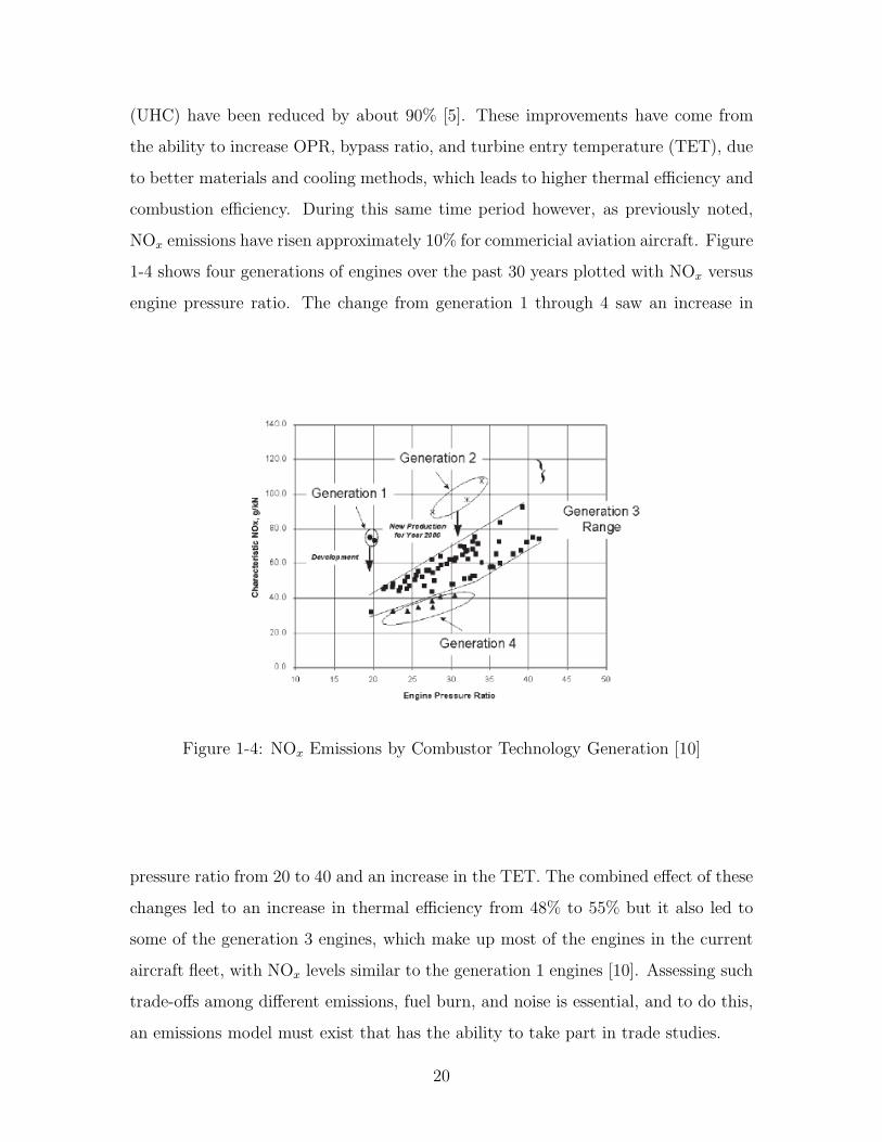
NOx emissions have risen approximately 10% for commericial aviation aircraft. Figure
1-4 shows four generations of engines over the past 30 years plotted with NOx versus
engine pressure ratio. The change from generation 1 through 4 saw an increase in
Figure 1-4: NOx Emissions by Combustor Technology Generation [10]
pressure ratio from 20 to 40 and an increase in the TET. The combined effect of these
changes led to an increase in thermal efficiency from 48% to 55% but it also led to
some of the generation 3 engines, which make up most of the engines in the current
aircraft fleet, with NOx levels similar to the generation 1 engines [10]. Assessing such
trade-offs among different emissions, fuel burn, and noise is essential, and to do this,
an emissions model must exist that has the ability to take part in trade studies.
20
1.2 Necesssary Attributes of an Emissions Model
for Policy Making
For an emissions model to assess trade-offs between different emissions as well as
the effects of potential future combustor designs, the model should have three fea-
tures. The emissions model should represent the physical relationships between op-
erating conditions, simplified combustor design parameters, and pollutant emissions
in a consistent way. The model should have as inputs, high-level design parameters
and operating conditions that would be convienient for an expert to use in projecting
future technology. For example, overall fuel-air ratio and inlet pressures and tem-
peratures are more appropriate than detailed specifications of cooling flow geometry
and recirculation zone patterns. The model should be general, meaning one modeling
methodology can be applied to estimate broad trends in combustor designs across
engine manufacturers.
1.3 Current Emissions Prediction Strategies and
Techniques
There are currently several techniques used in practice to predict the emissions of
aircraft gas turbine combustors. These techniques fall into four general catagories,
empirical models, semiempirical models, simplified physics-based models, and high-
fidelity simulations. Each method has its strengths and weaknesses and each will be
discussed in turn.
1.3.1 Empirical Models
Empirical models tend to be the simplest of the four model types and the least com-
putationally intensive. They are defined here as any emissions model which requires
empirically determined constants along with any engine specific conditions (P3, T3,
mass flow-rate, fuel flow-rate, etc). These models are used mainly for NOx emissions
21

and are useful for correlating known historical NOx emissions for a specific combustor.
Equations 1.3 and 1.4 are examples of typical empirical NOx models.
EINOx = 0.0042
(
P3
439
).37
exp
(
T3 − 1471
345
)
T4, (1.3)
where P3 is the total pressure at the combustor inlet in psia, T3 is the total tempera-
ture at the combustor inlet in oR, and T4 is the total temperature at the combustor
exit in oR [11].
EINOx = 0.068P .53
exp
(
T3 − 459.67
345
)
exp (humFact × 0.0027114) (1.4)
where P3, T3, and T4 are defined as before and humFact is a humidity factor that
depends on altitude. At sea level, humFact = 0.0063 [11]. These two commonly used
empirical models for NOx show that this type of model usually uses only P3, T3, and
occasionally T4 as inputs. Relative humidity is incorporated by including a humidity
factor, as in equation 1.4, or by using the Boeing method 2 (BM2) approach [12].
The two empirical models shown above are used for single annular combustors
(SAC). Within this group of combustors, NOx models are generated by fitting em-
pirical constants using the certification data of a combustor. In general, an empirical
model can be fit to a single annular combustor using
EINOx = β1P.43
exp
(
T3
β2
)
, (1.5)
by fitting the β coefficients using a least squares approach. Using this technique, each
combustor within a given design family will have its own empirical NOx model that
will predict the NOx emission index for that combustor. The prediction will generally
be very good within the range of data used to generate the empirical constants. Dif-
ferent families of combustors have different general forms for empirical NOx models.
Equations 1.6 and 1.7 are empirical NOx models for dual annular combustors and
22
lean-premix-prevaporize (LPP) combustors respectively. Both are from [11].
EINOx = 3.9P .373 exp
(
T3 − 459.67
349.90
)
×exp(humFact×0.002114)×FAR/delphi (1.6)
where P3, T3, and humFact are defined as before and FAR is the fuel-air ratio of the
combustor and delphi is a variable that modifies the FAR for different cooling flow
regimes. This model is more complex than the simple model for the SAC and may
be better described as a semiempirical model. The LPP model is
EINOx = 0.0000758(P3 × 6.8948)0.75
√
0.0075T3
T4
(1.7)
where P3, T3, and T4 are all defined as before. There are similar models for rich-
quench-lean (RQL) combustors, staged-dual annular combustors, double dome com-
bustors and others. In all cases there is a general form of the empirical model and
coefficients are fit on an individual basis for specific combustors.
For situations where the combustor of an engine is fixed and certification data
are available, empirical models are easy to generate and are generally regarded as
more accurate when applied to engines for which they were derived but not for other
engines. Inputs to these models are usually based on P3 and T3, which are easily
estimated using performance specifications quoted by manufacturers and thus pro-
prietary data is unnecessary. The weaknesses of these types of models are that they
are not as accurate when used more generally and that they are useful for predict-
ing emissions only within the bounds of the historical databases on which they are
generated. When an empirical model is used for a large variety of combustors within
a single family using only a single set of empirical constants, the correlation with
any particular combustor tends to be poor. This makes it difficult to use empirical
modeling techniques unless an empirical model is generated for every combustor that
is to be studied. Since empirical models are generated from fitting a certain number
of constants using historical certification data, they cannot be expected to perform
as well when the combustor undergoes a design change.
Currently, empirical models for NOx are used in most large scale engine per-
23

formance tools (NPSS, NEPP). Each combustor will usually have its own empirical
model and the models are not typically used for analyzing the effects of design changes.
Another weakness of empirical models is that they do not exist for prediction of CO
emissions. This makes it impossible to capture consistent trades between NOx and
CO with empirical modeling techniques, which makes empirical models inadequate
for use in a policy-making emissions model.
1.3.2 Semiempirical Models
Semiempirical models consist of equations that contain empirically determined con-
stants, cycle parameters, and experimentally gathered data on residence times, char-
acteristic kinetic times, and other parameters like primary zone temperature. These
methods are capable of modeling CO emissions as well as NOx emissions with sepa-
rate correlations, which may nor may not be consistent with one another. Equation
1.8 is an example of a semiempirical model for carbon monoxide,
EICO = 35 × τCO/τsl,CO, (1.8)
where τCO is a characteristic kinetic time based on a reaction rate constant, and
τsl,CO is a characteristic quenching time, based on a measured quench length where
the overall equivalence ratio of the combustor drops below a certain value, causing
the temperature to drop below a critical value that hinders CO oxidation to CO2 [13].
Equation 1.9 is an example of a semiempirical model for NOx prediction.
EINOx =AVcP
1.2exp(0.009Tpz)
mATpz(∆P/P )0.5, (1.9)
where A is a constant, Vc is the combustor primary zone volume, P is pressure, Tpz
is the primary zone temperature, mA is the primary zone air flow rate, and ∆P is
the liner pressure drop [14]. Generally empirical models for NOx emissions are used
in favor of semiempirical models by industry and in tools like NEPP and NPSS.
A weakness of the semiempirical modeling approach is that the outputs, EICO
24
and EINOx, are very sensitive to the inputs and the inputs are very difficult to obtain,
particularly in the case of EICO. Since the relations for different emissions are not
related to one another in any way, which could lead to inconsistent predictions of NOx
and CO, and since the models frequently require experiment or expert knowledge of
a particular combustor for use, these types of models do not meet the requirements
for use in a policy making tool. These models also have limited use for predicting
the effects of combustor design changes on emissions because the effects of a design
change on the model inputs would likely not be known unless the design change has
already been tested physically.
1.3.3 Simplified Physics-Based Models
Simplified physics-based models consist of reduced-order physics and chemistry in
ideal reactors aimed at using physical parameters to get useful results at a fraction of
the computational burden of a more detailed simulation. These types of models are
not widely used for emissions prediction. A weakness of using a simplified physics-
based model is that it is possible to get accurate estimates of emissions with a model
that is not accurately capturing the physics and chemistry of the combustion process.
For example, if a physics-based model does not incorporate two phenomena with
opposite effects on a particular output, then in cases where the effects cancel out, the
physics-based model will provide a good estimate of the output, but in cases where
the effects do not cancel out, the physics-based model will not provide a good estimate
of the output. This situation, however, is difficult to account for with a simplified
physics-based model. Simplified physics-based models and the ideal reactors of which
they consist will be discussed in greater detail in Chapter 2.
1.3.4 High Fidelity Simulations
High fidelity simulations use grids with millions of points, detailed kinetic mecha-
nisms, large eddy simulations (LES), and complex 3D geometries to estimate the
products of gas turbine combustion. High-fidelity simulations have been used effec-
25

tively for some aspects of combustor design, however, they are very computationally
intensive, and require detailed knowledge of combustor geometry and operating con-
ditions. Table 1.1 provides data from a NASA Glenn simulation of a GE90 engine to
Component No. of Iterations No. of Processors Wall clock timeCombustor 31000 256 3 hr 53 min
Table 1.1: Full Simulation Time [15]
predict temperature and velocity fields. The table shows that the time and computing
power required for this sort of approach is too great for use in a policy making tool.
Furthermore, high-fidelity simulations require detailed definitions of the combustor
designs, which would not be available for assessing technology trade-offs for potential
future combustor designs.
1.3.5 State of the Art for Emissions Trade Analyses
Currently, empirical models are used more than any other type of model because they
are general and computationally inexpensive. For trade studies and design change
analyses however, empirical models are less useful. Semiempirical models exist to
some extent on an individual combustor basis for both NOx and CO, but the inputs
to these models are typically not available when considering the impacts of alterna-
tive emissions policies on future engine and combustor configurations. Semiempirical
models also would have limited capability for studying the effects of design changes
that have not yet been measured. Physics-based models have been shown to have
some potential for capturing the interdependencies of emissions as well as combustor
performance on a very specific basis. Most of the work done with these models has
focused on creating a model to predict the emissions of a single combustor and has
not been extended in a general way. Full simulations require detailed definitions of
the geometry and operating conditions and are computationally prohibitive.
26

1.4 A Physics-Based Emissions Model
Given that the physics-based model has the most potential for a general emissions
model for a policy tool, a simplified physics-based model was selected for further
study to determine whether or not a model of that nature could be developed to
meet the three requirements for a policy-making tool referred to in Section 1.2.
1.4.1 Objective
The objective of this research is thus to create a physics-based model for estimating
emissions of potential future gas turbine combustors within quantified uncertainty
bounds. The method should be capable of predicting various tradeoffs associated
with typical changes in the design of a combustor. The emissions model is being
designed for use as a component of a policy-making tool, and as such, higher levels
of uncertainty are acceptable than would be the case if the model was for use in the
design of a combustor.
1.4.2 Emissions Model Success Criteria
The success of the emissions model developed in this thesis is measured by how
well the three attributes that make a model suitable for use in a policy making tool
are incorporated. The physical relationships among operating conditions, simplified
combustor design parameters, and pollutant emissions are assessed by comparing the
response of the model emissions outputs to different operating conditions and design
parameters to the response that would be expected from theory or the response that
is apparent in certification data. A successful model should predict trends that are
supported by theory and data. The high-level design parameters and operating con-
ditions that would be convienient for an expert to use in projecting future technology
should be built into the model as inputs. How well the model predicts broad trends
in the emission levels from different combustor designs is determined by how well the
model performs relative to an empirical model for NOx, and whether or not the model
predictions are within the uncertainty in the certification data for CO. The goal is to
27

produce estimates of the trends in emissions of NOx and CO at a level of accuracy
that is valuable in a policy-making setting. In particular, it is desired first that the
correct sign be predicted for changes in emissions with design and operating param-
eters. If this level of performance is met, an additional goal is to predict changes in
emissions with changes in design and operating conditions with an accuracy that ap-
proaches that of the uncertainty and variability of measurements of emissions indices
for the active fleet (e.g. about 16% for NOx and 23% for CO). Detailed data from
five industry combustors were used in the assessment of the model.
1.5 Thesis Outline
Chapter 2 discusses the development of the physics-based emissions models used in
the study. Chapter 3 focuses on how primary zone unmixedness is set in the model.
Chapter 4 compares the response of the model emissions outputs to changing oper-
ating conditions and combustor design parameters. Chapter 5 presents a comparison
of the emissions levels predicted by the model to the ICAO certification data and an
empirical model for five different engines. The model’s ability to predict the effects of
a design change is also assessed in Chapter 5. Chapter 6 contains general conclusions
about the work as well as a discussion of future work that should be done.
28

Chapter 2
Developing a Physics-Based
Emissions Model
This chapter discusses the developement of a physics-based emissions model for single
annular aircraft gas turbine combustors. The functional requirements of the model
are discussed followed by the inputs and outputs of the model. Fundamentals of
combustion are then reviewed to introduce the governing equations followed by a
discussion of ideal reactors. The use of ideal reactors to model each zone of a gas
turbine combustor is then discussed.
2.1 Functional Requirements
The physics-based emissions model should have as inputs, high-level design param-
eters and operating conditions that would be convienient for an expert to use in
projecting future technology. The emissions model should also represent the physical
relationships among operating conditions, combustor design parameters, and pollu-
tant emissions in a consistent way. The model must also produce estimates of the
trends in emissions of NOx and CO at a level of accuracy that is valuable in a policy-
making setting. In particular, it is desired first that the correct sign be predicted for
changes in emissions with design and operating parameters. If this level of perfor-
mance is met, an additional goal is to predict changes in emissions with changes in
29
design and operating condtions with an accuracy that approaches that of the uncer-
tainty and variability of measurements of emissions indices for the active fleet (e.g.
about 16% for NOx and 23% for CO).
2.2 Model Input/Output
The inputs to the physics-based emissions model are the combustor inlet temperature
and pressure, the mass flow rate into the combustor, the fuel flow rate, the mass flow
splits, the combustor zone volumes, and the primary zone unmixedness. The inputs
are all useful and convienient for expert use and contain the physical relationships
between operating conditions and combustor design parameters.
The chemical kinetics taking place in the combustion process are modeled with
the Gas Research Institute mechanism (GRImech) version 3.0 for propane [16]. Us-
ing GRImech v3.0 ensures that the physical relationships between gaseous pollutant
emissions and combustor design parameters and operating conditions are accounted
for in a consistent manner.
The outputs from the model are the emissions indices of NOx (EINOx) and CO
(EICO).
2.3 Combustion Fundamentals
Combustion in a gas turbine engine consists of the rapid oxidation of a fuel, which
generates heat. For gas turbine combustion, the oxidizer is typically air and the fuel
may be liquid or gaseous [14]. The combustion of a fuel-air mixture in an aircraft
engine is a complex, unsteady, turbulent process governed by a set of non-linear
partial differential equations.
30
2.4 Governing Equations
The governing equations are the conservation of mass, species, momentum, and energy
for a reacting flow. The most general form of mass conservation for a fixed point in
a flow may be written as∂ρ
∂t+ ∇ · (ρu) = 0, (2.1)
where ρ is density and u is velocity. The general form of species conservation for a
reacting flow may be written as
∂(ρYi)
∂t+ ∇ · m′′
i = m′′′
i for i = 1,2,...,N, (2.2)
where Yi is the mass fraction of species i, m′′
i is the mass flux of species i, and m′′′
i is
the net rate of mass production of species i per unit volume. The first term on the
left of Equation 2.2 is the rate of increase of mass of species i per unit volume. The
second term is the net rate of mass flow of species i out by diffusion and bulk flow
per unit volume [17]. The conservation of momentum in general form for a reacting
flow may be written as
ρDui
Dt= −
∂p
∂xi
+ ρgi +∂
∂xj
[
2µeij −2
3µ(∇ · u)δij
]
, (2.3)
which is a general form of the Navier-Stokes equation. The compressible form of the
conservation of momentum must be used because large changes in density can occur
in a reacting flow. The unsteady term must be kept because most flows within a
gas turbine combustor are turbulent. In Equation 2.3, u is velocity, p is pressure,
g is gravitational acceleration, µ is dynamic viscosity, eij is the strain rate tensor,
eij ≡ 1
2
(
∂ui
∂xj+
∂uj
∂xi
)
, and δij is the Kronecker delta. The conservation of energy in
one dimension may be written as
∑
m′′
i
dhi
dx+
d
dx
(
−kdT
dx
)
+ m′′ux
dux
dx= −
∑
him′′′
i , (2.4)
31

where hi is the specific enthalpy of species i, k is the thermal conductivity and ux is
the velocity in the x direction.
The simultaneous solution of these four coupled, non-linear, partial differential
equations, (with an appropriate model for turbulence and the kinetic relations for
the chemical species), could in theory be solved to provide estimates of species con-
centrations. Since a detailed geometry definition is required to solve such a problem,
the governing equations are too general to meet the objectives of a physics-based
emissions model for a policy making tool. To create a physics-based model of gas
turbine combustion that does not require detailed geometric specifications, several
assumptions that reduce the level of complexity of the governing equations must be
made.
2.5 Reducing the Governing Equations
The full set of governing equations includes several aspects of reacting flows that may
be neglected if higher levels of uncertainty in the emissions estimates are acceptable.
Ideal reactors such as perfectly stirred reactors and plug flow reactors make a number
of assumptions that significantly reduce the complexity of the combustion process
while still providing useful information.
2.5.1 The Perfectly Stirred Reactor
The perfectly stirred reactor (PSR) is an ideal reactor that neglects mixing phenomena
in a reaction. Combustion processes are characterized by the characteristic times
certain processes take. In a system where either the mixing rates are high or the
chemical reaction rates are slow, the chemical kinetics constrain the burning rates in
the mixture. The situation may be characterized by a Damkohler number, Da. The
Damkohler number is defined as
Da ≡τflow
τchem
, (2.5)
32

where τflow is a characteristic mixing time and τchem is a characteristic chemical time
[18]. In situations where Da ≪ 1, the burning rate is almost completely dependent
on the chemical kinetics of the mixture. When this is the case, calculations that
ignore mixing phenomena, like convection and diffusion, and focus only on the kinetic
modeling may be used.
The perfectly stirred reactor (PSR) assumes that the Damkohler number is essen-
tially zero and thus the mixture is considered perfectly stirred. Mixing has no effect
on the system and is not included in the calculations. This assumption allows for a
large reduction in the complexity of the governing equations.
Conservation Equations for the PSR
Following Turns [17], the conservation equations for the perfectly stirred reactor may
be written as follows. The control volume for the analysis is shown in Figure 2-1.
Mass conservation for an arbitrary species i may be written as
Figure 2-1: Diagram of a Perfectly Stirred Reactor, adapted from [17]
0 = m′′′
i ∀ + mi,in − mi,out, (2.6)
33

where m′′′
i ∀ is the rate of generation or destruction of mass of the ith species, ∀ is
the volume, mi,in is the mass flow of the ith species into the control volume, and
mi,out is the mass flow of the ith species out of the control volume. The generation or
destruction of a species is written as
m′′′
i = ωiMWi, (2.7)
where ωi is the net production rate of the ith species in mol/m3s and MWi is the
molecular weight of the ith species in kg/mol. The mass flow of the ith species into
the control volume is the mass flow in multiplied by the initial mass fraction of the
species, or
mi,in = mYi,in (2.8)
and similarly, the mass flow out of the control volume is
mi = mYi. (2.9)
The mass fraction of a species is the individual mass of the ith species in the mixture
divided by the total mass of the mixture.
The conservation of energy for the perfectly stirred reactor may be written as
Q = m(hout − hin). (2.10)
In terms of the individual species this is
Q =
(
N∑
i=1
Yi,outhi(T ) −
N∑
i=1
Yi,inhi(Tin)
)
, (2.11)
where hi is the specific enthalpy of the ith species, which is written as
hi(T ) = hof,i +
∫ T
Tref
cp,i(T )dT. (2.12)
34
The term hof,i is the enthalpy of formation of the ith species and cpi
(T ) is the specific
heat of the ith species, which is a function of the temperature of the mixture.
The Mathematical Simplicity of the Perfectly Stirred Reactor
Since there is no dependence on flow parameters there is no conservation of momentum
equation for the perfectly stirred reactor. Also, because the reactor is operating at
steady-state, there is no time dependence in the conservation equations. As a result
the perfectly stirred reactor is described fully by a set of coupled nonlinear algebraic
equations instead of a system of non-linear partial differential equations. The result
is that problems dealing with perfectly stirred reactor models may be solved using a
Newton-Raphson approach.
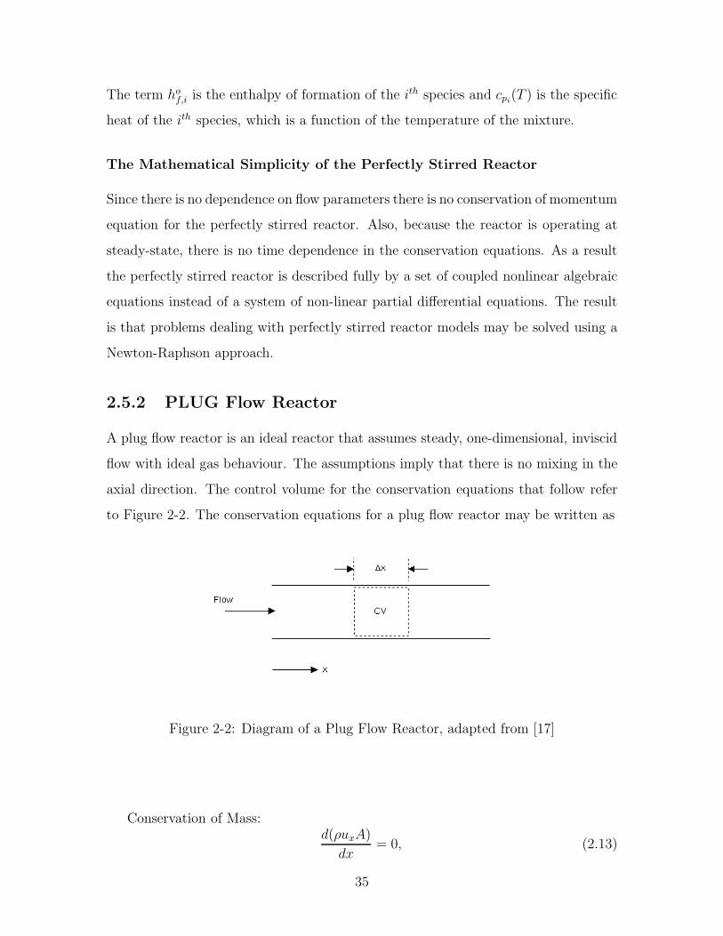
2.5.2 PLUG Flow Reactor
A plug flow reactor is an ideal reactor that assumes steady, one-dimensional, inviscid
flow with ideal gas behaviour. The assumptions imply that there is no mixing in the
axial direction. The control volume for the conservation equations that follow refer
to Figure 2-2. The conservation equations for a plug flow reactor may be written as
Figure 2-2: Diagram of a Plug Flow Reactor, adapted from [17]
Conservation of Mass:d(ρuxA)
dx= 0, (2.13)
35

Conservation of Momentum:
dp
dx+ ρux
dux
dx= 0, (2.14)
Conservation of Species:dYi
dx−
ωiMWi
ρux
= 0, (2.15)
Conservation of Energy:
dT
dx=
u2
x
ρcp
dρ
dx+
u2
x
cp
(
1
A
dA
dx
)
−1
uxρcp
n∑
i=1
hiωiMWi, (2.16)
The Mathematical Simplicity of the Plug Flow Reactor
The assumptions of the plug flow reactor reduce the coupled, non-linear, three-
dimensional governing equations of combustion to a set of coupled ordinary differential
equations, for which many efficient solution methods exist.
2.6 Modeling a Gas Turbine Combustor with Ideal
Reactors
A gas turbine combustor typically consists of a primary zone, an intermediate zone,
and a dilution zone. To represent the physical relationships among operating condi-
tions, pollutant emissions, and combustor design parameters like zone volumes, the
emissions model should be developed to capture the physical layout of a combustor.
2.6.1 The Role of the Primary Zone
The primary zone of a gas turbine combustor is designed to anchor the flame and
achieve nearly complete combustion of the fuel. To do this, the primary zone must
provide sufficient residence time for the fuel-air mixture, as well as high temperatures
and high turbulence for rapid mixing of the fuel and air. For these reasons primary
zones of typical combustors have large recirculation regions of flow, high temperatures,
36

and high levels of turbulence.
2.6.2 Modeling the Primary Zone
Regions of strong turbulence in a combustion process tend to have short characteristic
mixing times relative to the kinetic times. The result is that these regions have low
Damkohler numbers. This suggests that the primary zone could be modeled using a
PSR, which assumes instantaneous mixing with a Damkohler number of zero. Figure
2-3 shows the effects of increasing levels of turbulence intensity on Damkohler number
and how the combustion should be modeled. Turbulence intensity, Vt/Su, which is
the ratio of characteristic turbulence velocity to the laminar flame speed, is plotted on
the vertical axis, and a length scale ratio, lt/∆F , which is the ratio of the turbulence
length scale to the flame thickness, is plotted on the horizontal axis. The Damkohler
number is related to these scales by
Vt
Su
=1
Da
lt∆F
. (2.17)
Both the equation and the figure show that as turbulence intensity increases, the
Damkohler number decreases. The figure shows that as the Damkohler number de-
creases, the combustion process becomes more and more suitable for modeling with
a stirred reactor. With the high level of turbulence expected in the primary zone
for most engine power settings, the PSR has the potential for being an appropriate
model.
2.6.3 Primary Zone Emissions Considerations
Using only a single PSR to model the primary zone of a combustor implies that the
entire fuel-air mixture is perfectly mixed and remains so throughout the zone. In a
real combustor, however, fuel and air are injected separately, and this ideal situation
cannot be expected to prevail. This means that the Damkohler number is not likely
to be close enough to zero for a single PSR to be an adequate model for emissions of
NOx and CO, which are highly sensitive to the local fuel-air ratio in the combustor.
37

Figure 2-3: The Effect of Turbulence on Damkohler Number [18]
The activation energy of NOx is strongly dependent on temperature and thus on local
equivalence ratio. For CO, if the local equivalence ratio is greater than unity, large
amounts of CO will be formed due to lower oxygen concentration for completing the
reaction to CO2. For equivalence ratios close to unity, large amounts of CO will form
because of CO2 dissociation. For very low equivalence ratios (φ < 0.6), the mixture
strength cannot support complete combustion and CO is formed in great quantities
farther down the combustor. According to Lefebvre [14], only for equivalence ratios
of about 0.7-0.9 will low levels of CO be formed. Therefore, if CO emissions are to be
properly calculated, any deviation from a perfect mixture in the primary zone must
be accounted for to ensure that local equivalence ratios are correct. Due to these
considerations, the model of the primary zone should include some mechanism for
incorporating varying levels of unmixedness.
Modeling Unmixedness in the Primary Zone
A typical approach for capturing the unmixedness in a combustor is to assume that the
mixture can be approximated by a normal distribution about some mean equivalence
ratio [24]. The distribution is then defined by an unmixedness parameter, s, where
s =σφ
µφ
, (2.18)
38

and σφ is the standard deviation of the distribution and µφ is the mean equivalence
ratio. This technique has been used numerous times [19]. Figure 2-4 shows how the
0 0.2 0.4 0.6 0.8 1 1.2 1.4 1.6 1.8 20
0.05
0.1
0.15
0.2
0.25
0.3
0.35
Primary Zone Equivalence Ratio
Per
cent
of P
rimar
y Z
one
Mas
s F
low
Mean Equivalence Ratio = 1.0s = 0.25No. PSRs = 10
Figure 2-4: Normal Distribution of Equivalence Ratio in the Primary Zone PSRs
equivalence ratios and mass flow percentages through a set of 10 PSRs are set with
an unmixedness value of s = 0.25 and a mean equivalence ratio of φp = 1. The
equivalence ratios are determined using Equation 2.18 and the mass flow percentages
are calculated from the cumulative distribution function and are shown on the vertical
axis.
To determine how many PSRs should be used for the distribution, a variable
number of PSRs were run to represent the primary zone of a combustor, followed by
a PSR to represent the intermediate zone and a plug flow reactor to represent the
diluton zone. The inputs were taken from an industry gas turbine combustor. The
emissions output from the different cases were plotted to determine when adding more
PSRs no longer had a significant impact on the emissions indices. The outputs of
interest are the emissions indices of NOx and CO. The percentage change in emissions
indices for NOx and CO were calculated as
%∆EINOx(i + 1) =
EINOx(i + 1) − EINOx(i)
EINOx(i)(2.19)
%∆EICO(i + 1) =EICO(i + 1) − EICO(i)
EICO(i)(2.20)
39

where the values i and i+1 refer to the number of PSRs in the model and i = 1, ..., 39.
The number of PSRs was considered adequate when the percentage change with each
additional reactor in EINOx fell below 5% and the percentage change in EICO fell
below 15% for all four ICAO engine power settings. The reason for this was that the
90% confidence interval for new, uninstalled engines picked out of a fleet is ±16% for
EINOx and ±23% for EICO [20]. Since the desired accuracy of the model is to be
within the uncertainty in the data, the addition of more PSRs beyond the uncertainty
in the data has no impact on whether or not the objectives of the model will be met.
Stricter criteria than the uncertainty in the data were used because the values for
the uncertainty in the NOx and CO emissions data are considered conservative. The
results of the analysis are shown in Figure 2-5. The data was collected with an
0 5 10 15 20 25 30 35 400
10
20
30
40
50
60
70
80
90
100
Primary Zone Model Requirements for EINOx, s = 0.7
% C
hang
e in
EIN
Ox
Number of PSRs
IdleApproachClimbTakeoff
(a) EINOx
0 5 10 15 20 25 30 35 400
10
20
30
40
50
60
70
80
90
100Primary Zone Model Requirements for EICO, s = 0.7
% C
hang
e in
EIC
O
Number of PSRs
IdleApproachClimbTakeoff
(b) EICO
Figure 2-5: Determining the Primary Zone Model
unmixedness level of s = 0.7, which is the highest value of primary zone unmixedness
that is expected to occur [19]. Higher levels of unmixedness require more reactors to
appropriately reflect the normal distribution, which is why the unmixedness level was
chosen at the highest level. The plots show that for EINOx to be modeled adequately
with a normal distribution, there must be at least eleven PSRs in the primary zone.
For EICO to be modeled adequately, there must be at least sixteen PSRs in the
40
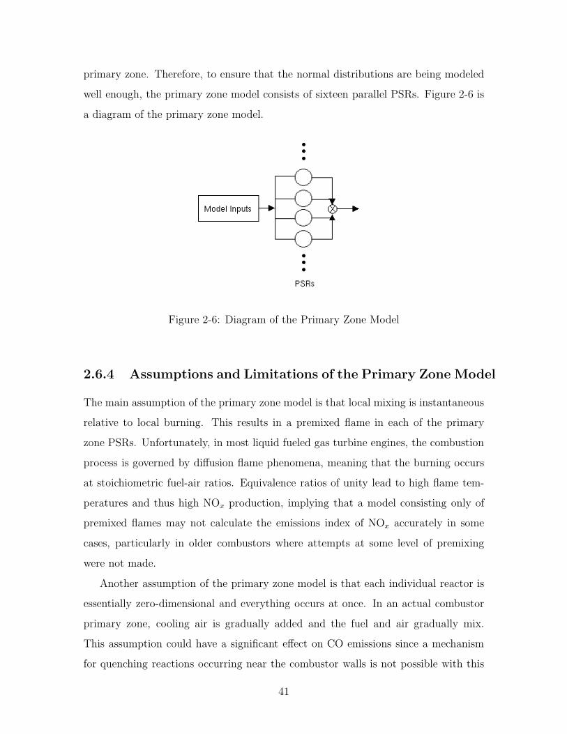
primary zone. Therefore, to ensure that the normal distributions are being modeled
well enough, the primary zone model consists of sixteen parallel PSRs. Figure 2-6 is
a diagram of the primary zone model.
Figure 2-6: Diagram of the Primary Zone Model
2.6.4 Assumptions and Limitations of the Primary Zone Model
The main assumption of the primary zone model is that local mixing is instantaneous
relative to local burning. This results in a premixed flame in each of the primary
zone PSRs. Unfortunately, in most liquid fueled gas turbine engines, the combustion
process is governed by diffusion flame phenomena, meaning that the burning occurs
at stoichiometric fuel-air ratios. Equivalence ratios of unity lead to high flame tem-
peratures and thus high NOx production, implying that a model consisting only of
premixed flames may not calculate the emissions index of NOx accurately in some
cases, particularly in older combustors where attempts at some level of premixing
were not made.
Another assumption of the primary zone model is that each individual reactor is
essentially zero-dimensional and everything occurs at once. In an actual combustor
primary zone, cooling air is gradually added and the fuel and air gradually mix.
This assumption could have a significant effect on CO emissions since a mechanism
for quenching reactions occurring near the combustor walls is not possible with this
41

model.
2.6.5 The Role of the Intermediate Zone
The intermediate zone of a combustor is designed to recover dissociation losses, burn
poorly mixed fuel-rich pockets at low altitude and serve as an extension of the primary
zone at high altitude. At low altitude, the high temperature conditions of the primary
zone lead to the dissociation of CO2 to CO. If the reaction is then quenched the CO
concentration will essentially be frozen, leading to high CO output. The intermediate
zone’s role is then to slowly add dilution and cooling air while maintaining a high
enough temperature to complete combustion. Pockets of fuel-rich mixture may also
exist leaving the primary zone which must be burned in the intermediate zone oth-
erwise there will be a penalty in combustion efficiency. At high altitude combustion
is usually not complete at the exit of the primary zone because the fuel-air concen-
tration is lower, due to lower pressure, which leads to reduced reaction rates. In this
case the combustion process continues in the intermediate zone. These requirements
lead to a trade off in the intermediate zone between zone length, which determines
the residence time, and combustion efficiency.
2.6.6 Modeling the Intermediate Zone
To determine how to best model the intermediate zone, six candidate intermediate
zone reactor setups were studied and the output of each model was compared to
emissions data. Six candidate reactor setups were studied because it was unclear
how to best model the intermediate zone. The six candidate reactor setups were a
single plug flow reactor, a single PSR, a set of parallel plug flow reactors, a set of
parallel PSRs, a bulk plug flow reactor with a wall plug flow reactor, and a bulk
plug flow reactor with a wall PSR. The single plug flow reactor was tested because it
would be an appropriate model if the mixing of fuel and air in the primary zone, as
well as added cooling air and dilution air prior to the intermediate zone, is complete.
For this situation the plug flow reactor could be used to simulate a one-dimensional
42
reacting flow. A single PSR was tested because it would be an appropriate model
if recirculation due to the addition of downstream dilution air and cooling air is
present in the intermediate zone. Parallel plug flow reactors and parallel PSRs were
tested because they would be a more appropriate model for the intermediate zone if
the effects of a non-uniform mixture, due to the addition of cooling air and dilution
air along the walls of the combustor, are significant in terms of emissions output.
Modeling the bulk flow with a single plug flow reactor and the flow near the walls
of the combustor intermediate zone, where CO is not likely to oxidize to CO2 due to
the lower temperatures, with a PSR or a plug flow reactor was tested because of the
possibility that most of the CO formed during combustion is due to quenching near
the walls of the combustor.
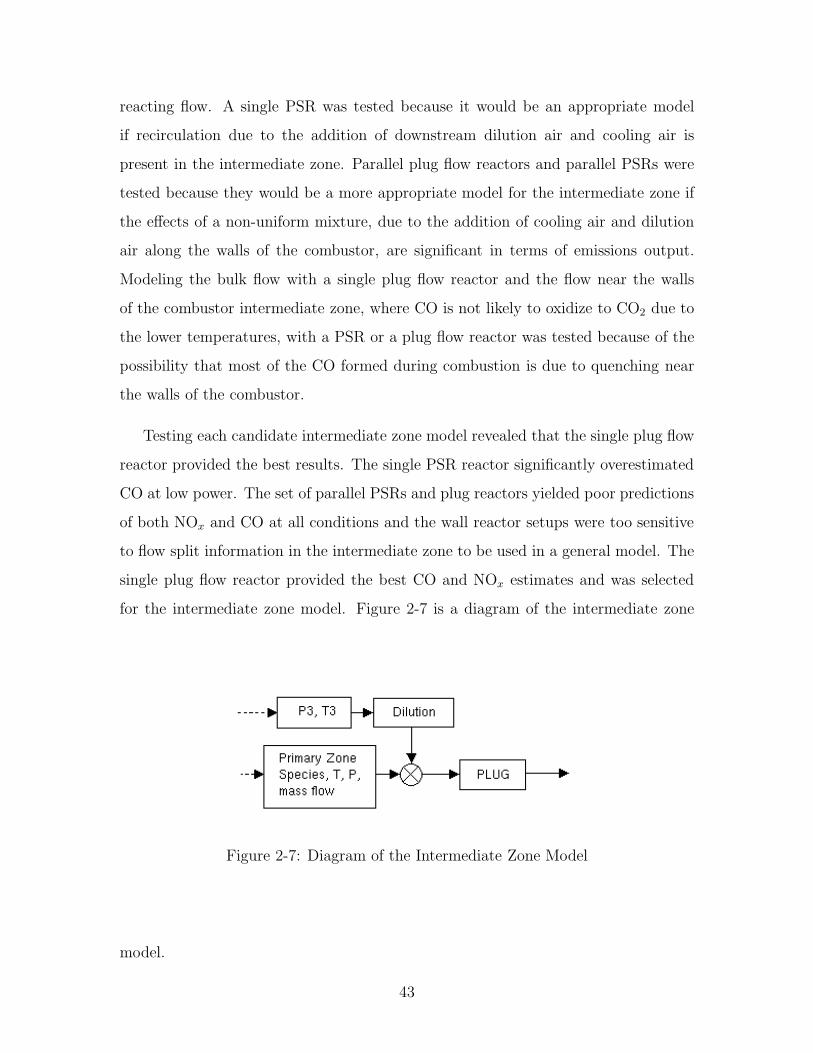
Testing each candidate intermediate zone model revealed that the single plug flow
reactor provided the best results. The single PSR reactor significantly overestimated
CO at low power. The set of parallel PSRs and plug reactors yielded poor predictions
of both NOx and CO at all conditions and the wall reactor setups were too sensitive
to flow split information in the intermediate zone to be used in a general model. The
single plug flow reactor provided the best CO and NOx estimates and was selected
for the intermediate zone model. Figure 2-7 is a diagram of the intermediate zone
Figure 2-7: Diagram of the Intermediate Zone Model
model.
43
2.6.7 Intermediate Zone Emissions Considerations
The formation of NO in a gas turbine combustor only proceeds at a significant rate at
temperatures above around 1800K [14]. Since these high temperatures are expected
to occur mainly in the primary zone, the effect of the intermediate zone model on NOx
emissions is negligible as seen in Chapter 4. Since the intermediate zone is designed
to complete the combustion of the mixture leaving the primary zone, the intermediate
zone oxidizes most of the CO to CO2.
2.6.8 Assumptions and Limitations of the Intermediate Zone
Models
The main assumption of the intermediate zone model is the instantaneous addition of
cooling air and dilution air. This is not expected to impact NOx output significantly,
but it may have an effect on CO emissions. Gradual air addition would allow for
higher zone temperatures, which would lead to more CO oxidation to CO2. The
assumption may therefore, lead to overestimates of CO emissions.
2.6.9 The Role of the Dilution Zone
The dilution zone of a gas turbine combustor is designed to bring the gas to an
acceptable mean temperature and to improve the pattern factor prior to the turbine
inlet. At most power conditions combustion has essentially been completed and the
emissions of NOx and CO are not changed. At low power it is possible that further CO
oxidation may take place but the addition of dilution air and cooling air will usually
reduce the temperature to the point where these reactions are no longer taking place.
2.6.10 Modeling the Dilution Zone
The flow in the dilution zone is essentially one-dimensionally moving towards the
turbine and should be modeled reasonably well with plug flow reactors. The model
for the dilution zone is thus two serial plug flow reactors, one for the initial addition
44

of dilution air, which could potentially have an impact on CO emissions, and another
for the addition of pattern factor cooling air. Figure 2-8 is a diagram of the dilution
Figure 2-8: Diagram of the Dilution Zone Model
zone model.
2.6.11 Modeling the Injection of Dilution/Cooling Air
Gas turbine combustors usually have two main forms of air addition that serve two
different purposes. Dilution air is usually injected in two major locations and its
purpose is to bring the gas temperature to the point where CO is still oxidizing to
CO2, but NOx is no longer being formed in major quantities, and also to reduce the
mean gas temperature prior to turbine entry. Cooling air is injected along both the
inner and outer diameter of the combustor liner and its purpose is to protect the liner
material from the hot temperatures of the reacting bulk flow. Where and how much
air is injected into the combustor is defined by flow splits and geometry, which define
where the flow is introduced into the combustor and what percentage of the total air
mass flow rate comes through each cooling slot and dilution hole. Figure 2-9 is an
example of a set of flow splits for a given combustor geometry. The letters in the
figure would be different percentages of mass flow rate entering at each location. The
difficulty with the flow split information is determining how to map the flow split
inputs from the physical domain to the model domain. The model consists of air
addition only at two main dilution points and a final cooling air addition point. The
challenge is thus to determine when the air flow from each of the physical injection
45

Figure 2-9: Typical Combustor Flow Splits
points mixes in with the bulk flow. Several possibilities for this were tested and it was
found that assuming the cooling air mixes into the bulk flow when it encounters a
dilution jet provides the best results. This means that in the model, the flow entering
at location D is combined with the flow from location F because the injection at
D is cooling air that has encountered a main dilution injection at location F. The
assumption allows for simple transitions from combustor to combustor even though
the geometries and flow splits are usually unique to individual combustors.
2.6.12 Assumptions and Limitations of Injection Mapping
A major assumption of the modeling of air addition into the combustor is that it
is not necessary to exactly match the geometry and flow split inputs of the physical
combustor in the model domain to calculate emissions of NOx and CO. However, since
CO emissions can in some cases be the result of CO from the primary zone becoming
entrained into the cool air along the liner and then failing to oxidize because of the
lower temperatures, the air addition model may lead to erroneous CO predictions in
some cases. This is because the model does not permit gradual addition of cooling air
along the walls of the combustor where the CO from the primary zone could become
entrained.
46

2.6.13 Model Implementation
The ideal reactors that make up the physics-based emissions model are run using
Chemkin version 4.0. The inputs, reactor linking, air addition, and output calcula-
tions are all done with Matlab.
2.6.14 The Physics-Based Emissions Model
Figure 2-10 is a diagram of the simple physics-based emissions model that was created.
The primary zone is modeled as a network of 16 parallel PSRs, the intermediate zone
is modeled as an injection of air followed by a plug flow reactor, and the dilution zone
is modeled as an injection of air followed by a plug flow reactor, followed by another
injection of air and another plug flow reactor.
Figure 2-10: Diagram of the Physics-Based Emissions Model
47

48

Chapter 3
Setting the Unmixedness
Parameter
All of the inputs to the physics-based emissions model are measured physical quanti-
ties with the exception of primary zone unmixedness. The primary zone unmixedness
is a physical parameter, but it is not typically measured by industry. The physical
nature of this parameter stems from the level of mixing between fuel and air that
occurs in the primary zone of the combustor. There are several different options for
how the unmixedness parameter can be set. Among these are setting the unmixed-
ness level as a constant value at all engine power settings, setting the unmixedness
level as a function of primary zone equivalence ratio and using the relation generally
across all engines, and setting the unmixedness level as a function of primary zone
equivalence ratio for each individual baseline combustor. Setting a single value of
unmixedness across all engine power settings assumes that the unmixedness is only
a function of primary zone geometry. Setting the unmixedness using a general rela-
tionship between unmixedness and primary zone equivalence ratio implies that the
unmixedness is only a function of the fuel-air ratio and is independent of geometry.
Setting the unmixedness as a function of primary zone equivalence ratio for each base-
line combustor assumes that the unmixedness could be a function of both geometry
and fuel-air ratio. Testing each method revealed that the unmixedness should be set
as a function of primary zone equivalence ratio for each individual baseline combustor
49

because the unmixedness is a function of both fuel-air ratio and combustor primary
zone geometry.
3.1 Industry Data
Industry data were used to study the effects of the unmixedness parameter and how
it is set. The data came from five different combustors on five different gas turbine
engines in the same engine line. Table 3.1 gives the relative power of each engine and
how the engines are labeled in the study. Engine 1a is the result of a design change
Engine 1 Engine 1a Engine 2 Engine 3 Engine 3aRelative Power Medium Medium Low High High
Table 3.1: Relative Power of Each Engine in the Study
on Engine 1 and Engine 3a is the result of a design change on Engine 3.
3.2 Sensitivity to Unmixedness
To determine the impact of the unmixedness parameter on the model output, the
sensitivity of NOx and CO emissions to primary zone unmixedness was studied at
each ICAO LTO-cycle point. The unmixedness parameter was varied from 0 to 0.7
at all four power settings for Engine 1a. The results are shown in Figure 3-1. Given
that the emissions of NOx and CO are strong functions of unmixedness, particularly
for idle CO, the method of setting unmixedness is crucial to meeting the objective of
estimating emissions within the uncertainty in the certification data.
3.2.1 Single Value Optimization
Using a single value for the primary zone unmixedness of a combustor is useful if the
unmixedness parameter is set largely by the geometry of the combustor. That is, if
the unmixedness parameter is determined almost entirely by the injection methods
and the locations of air and fuel injection in the primary zone. If the assumption that
50

0 0.1 0.2 0.3 0.4 0.5 0.6 0.70
1
2
3
4
5
6
EIN
Ox g
/kg
fuel
0 0.1 0.2 0.3 0.4 0.5 0.6 0.70
100
200
300
400
500
Primary Zone Unmixedness
EIC
O g
/kg
fuel
NOx
CO
(a) Idle
0 0.1 0.2 0.3 0.4 0.5 0.6 0.70
4
8
12
16
EIN
Ox g
/kg
fuel
0 0.1 0.2 0.3 0.4 0.5 0.6 0.70
1
2
3
4
5
Primary Zone Unmixedness
EIC
O g
/kg
fuel
NOx
CO
(b) Approach
0 0.1 0.2 0.3 0.4 0.5 0.6 0.70
2
4
6
8
10
12
14
16
EIN
Ox g
/kg
fuel
0 0.1 0.2 0.3 0.4 0.5 0.6 0.70
0.05
0.1
0.15
0.2
0.25
0.3
Primary Zone Unmixedness
EIC
O g
/kg
fuel
NOx CO
(c) Climb Out
0 0.1 0.2 0.3 0.4 0.5 0.6 0.70
6
12
18
24
EIN
Ox g
/kg
fuel
0 0.1 0.2 0.3 0.4 0.5 0.6 0.70
0.06
0.12
0.18
Primary Zone Unmixendess
EIC
O g
/kg
fuel
NOx
CO
(d) Takeoff
Figure 3-1: Response of Engine 1a Emissions to Varying Unmixedness
51

the parameter is set largely by geometry is correct, then a single value of unmixed-
ness should work well across different engine settings and combustors with similar
geometries.
Setting the unmixedness to a single value is done by optimizing the unmixedness
so as to minimize the difference between model and ICAO Dp/Foo for both NOx and
CO. The differences in Dp/Foo for NOx and CO were calculated using Equations 3.1
and 3.2. The objective function for the optimization is given in Equation 3.3.
∆Dp/Foo NOx = ICAO Dp/Foo NOx − Model Dp/Foo NOx (3.1)
∆Dp/Foo CO = ICAO Dp/Foo CO − Model Dp/Foo CO (3.2)
f =(∆Dp/Foo NOx)
2 + (∆Dp/Foo CO)2
ICAO Dp/Foo NOx + ICAO Dp/Foo CO(3.3)
The results of using this method for calculating the unmixedness for the five industry
combustors are given in Table 3.2. The combustors used in the analysis are all
Engine 1 Engine 1a Engine 2 Engine 3 Engine 3aUnmixedness 0.30 0.02 0.34 0.19 0.27
Table 3.2: Single Value Optimized Unmixedness
very similar geometrically so the differences between the unmixedness values of each
combustor suggest that the parameter should not only be set by geometry.
3.2.2 General Curve Optimization
To set a general curve for the unmixedness parameter, unmixedness was optimized
at each ICAO LTO certification point for each engine. Following Sturgess, the un-
mixedness values were then fit with a polynomial as a function of equivalence ratio
[19]. This technique is useful if the unmixedness is not a function of geometry but
only a function of primary zone equivalence ratio. The objective function for these
52
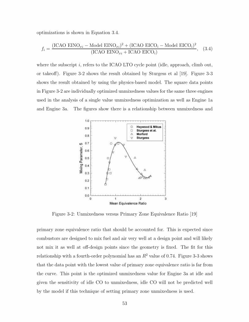
optimizations is shown in Equation 3.4.
fi =(ICAO EINOxi − Model EINOxi)
2 + (ICAO EICOi − Model EICOi)2
(ICAO EINOxi + ICAO EICOi), (3.4)
where the subscript i, refers to the ICAO LTO cycle point (idle, approach, climb out,
or takeoff). Figure 3-2 shows the result obtained by Sturgess et al [19]. Figure 3-3
shows the result obtained by using the physics-based model. The square data points
in Figure 3-2 are individually optimized unmixedness values for the same three engines
used in the analysis of a single value unmixedness optimization as well as Engine 1a
and Engine 3a. The figures show there is a relationship between unmixedness and
Figure 3-2: Unmixedness versus Primary Zone Equivalence Ratio [19]
primary zone equivalence ratio that should be accounted for. This is expected since
combustors are designed to mix fuel and air very well at a design point and will likely
not mix it as well at off-design points since the geometry is fixed. The fit for this
relationship with a fourth-order polynomial has an R2 value of 0.74. Figure 3-3 shows
that the data point with the lowest value of primary zone equivalence ratio is far from
the curve. This point is the optimized unmixedness value for Engine 3a at idle and
given the sensitivity of idle CO to unmixedness, idle CO will not be predicted well
by the model if this technique of setting primary zone unmixedness is used.
53
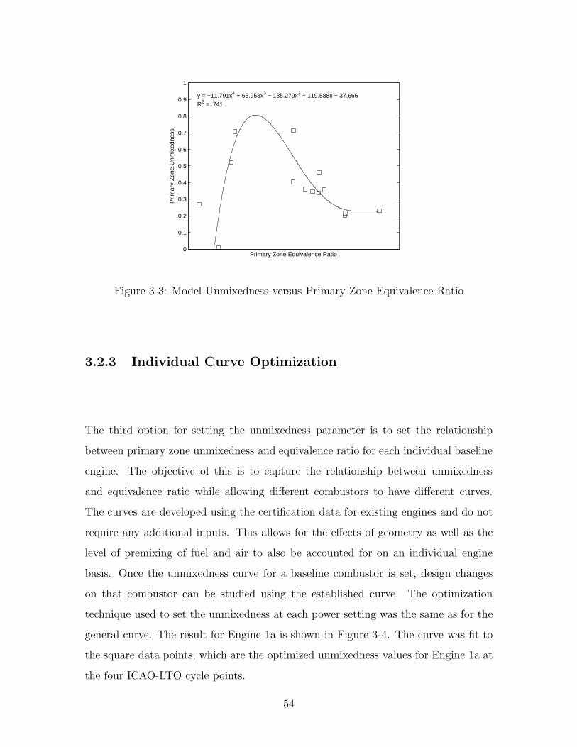
0
0.1
0.2
0.3
0.4
0.5
0.6
0.7
0.8
0.9
1
Primary Zone Equivalence Ratio
Prim
ary
Zon
e U
nmix
edne
ss
y = −11.791x4 + 65.953x3 − 135.279x2 + 119.588x − 37.666R2 = .741
Figure 3-3: Model Unmixedness versus Primary Zone Equivalence Ratio
3.2.3 Individual Curve Optimization
The third option for setting the unmixedness parameter is to set the relationship
between primary zone unmixedness and equivalence ratio for each individual baseline
engine. The objective of this is to capture the relationship between unmixedness
and equivalence ratio while allowing different combustors to have different curves.
The curves are developed using the certification data for existing engines and do not
require any additional inputs. This allows for the effects of geometry as well as the
level of premixing of fuel and air to also be accounted for on an individual engine
basis. Once the unmixedness curve for a baseline combustor is set, design changes
on that combustor can be studied using the established curve. The optimization
technique used to set the unmixedness at each power setting was the same as for the
general curve. The result for Engine 1a is shown in Figure 3-4. The curve was fit to
the square data points, which are the optimized unmixedness values for Engine 1a at
the four ICAO-LTO cycle points.
54

0
0.1
0.2
0.3
0.4
0.5
0.6
0.7
Primary Zone Equivalence Ratio
Prim
ary
Zon
e U
nmix
edne
ss
FitEngine 1a
y = 4.10x3 − 16.30x2 + 20.60x − 7.82R2 = 1.00
Figure 3-4: Model Unmixedness versus Primary Zone Equivalence Ratio for LTOCycle
3.3 Evaluating the Different Options
To determine which method of setting the unmixedness is most appropriate, the single
point method and the individual curve method were used to set the unmixedness
for Engine 1a using the known emissions data for that engine. The unmixedness
calculations from Engine 1a were then used on Engine 1 in the same manner that
they would be if one were trying to predict the impacts of the design change from
Engine 1a to Engine 1. The emissions data for Engine 1 were then used to calculate
individually optimized unmixedness values at each engine setting and the results were
compared to each method of setting unmixedness.
3.3.1 Single Point Estimate
Using the single point optimization on Engine 1a yields an unmixedness value of
s = 0.02. To study the effects of the design change from Engine 1a to Engine 1, the
unmixedness value calculated for Engine 1a is assumed to be valid for Engine 1 at all
power settings. Table 3.3 compares the optimized unmixedness values for Engine 1
using the certification data and the value of unmixedness calculated from Engine 1a.
55
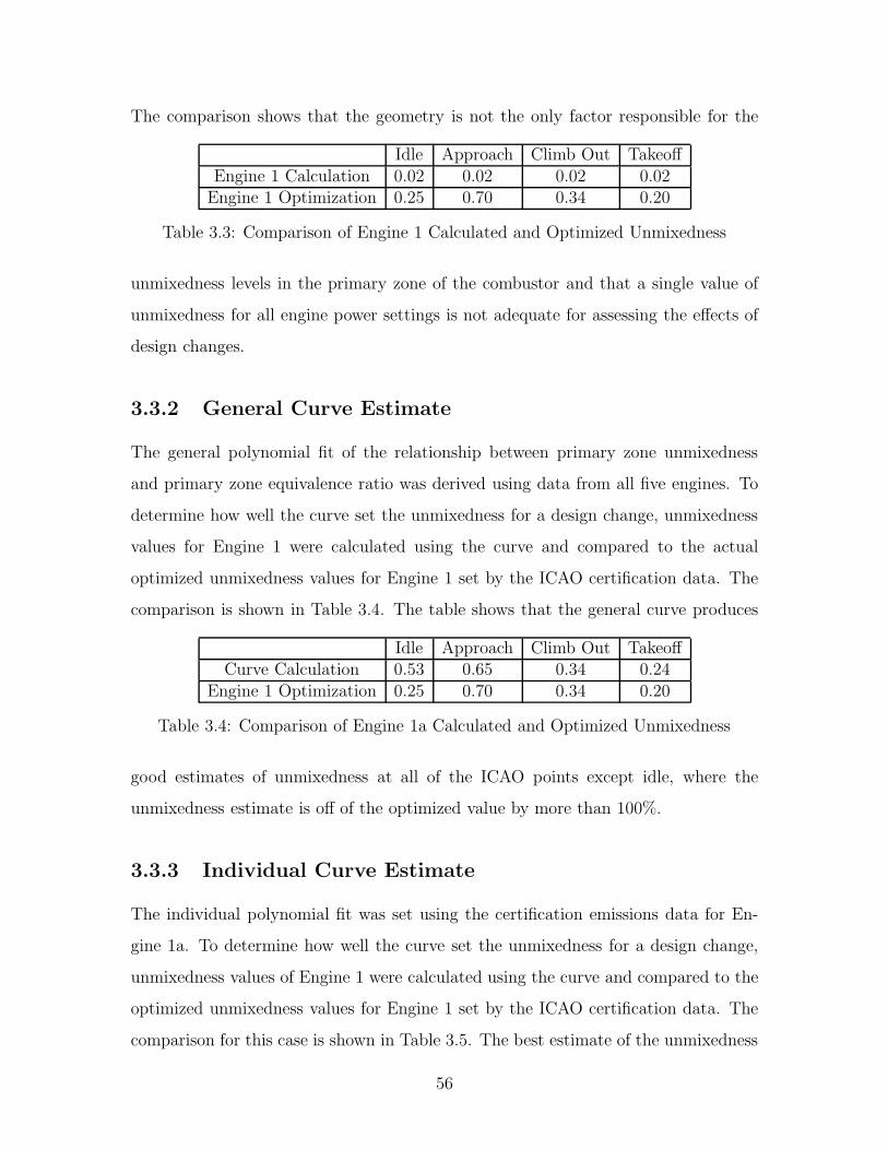
The comparison shows that the geometry is not the only factor responsible for the
Idle Approach Climb Out TakeoffEngine 1 Calculation 0.02 0.02 0.02 0.02
Engine 1 Optimization 0.25 0.70 0.34 0.20
Table 3.3: Comparison of Engine 1 Calculated and Optimized Unmixedness
unmixedness levels in the primary zone of the combustor and that a single value of
unmixedness for all engine power settings is not adequate for assessing the effects of
design changes.
3.3.2 General Curve Estimate
The general polynomial fit of the relationship between primary zone unmixedness
and primary zone equivalence ratio was derived using data from all five engines. To
determine how well the curve set the unmixedness for a design change, unmixedness
values for Engine 1 were calculated using the curve and compared to the actual
optimized unmixedness values for Engine 1 set by the ICAO certification data. The
comparison is shown in Table 3.4. The table shows that the general curve produces
Idle Approach Climb Out TakeoffCurve Calculation 0.53 0.65 0.34 0.24
Engine 1 Optimization 0.25 0.70 0.34 0.20
Table 3.4: Comparison of Engine 1a Calculated and Optimized Unmixedness
good estimates of unmixedness at all of the ICAO points except idle, where the
unmixedness estimate is off of the optimized value by more than 100%.
3.3.3 Individual Curve Estimate
The individual polynomial fit was set using the certification emissions data for En-
gine 1a. To determine how well the curve set the unmixedness for a design change,
unmixedness values of Engine 1 were calculated using the curve and compared to the
optimized unmixedness values for Engine 1 set by the ICAO certification data. The
comparison for this case is shown in Table 3.5. The best estimate of the unmixedness
56

Idle Approach Climb Out TakeoffCurve Calculation 0.40 0.46 0.38 0.25
Engine 1 Optimization 0.25 0.70 0.34 0.20
Table 3.5: Comparison of Engine 1a Calculated and Optimized Unmixedness
value at idle is obtained using this method. The approach estimate is not as good
as the general curve approach estimate, but the sensitivity of the emissions outputs,
particularly CO, are much higher at idle, as shown in Figure 3-1.
3.4 Setting Unmixedness
To meet the objectives of the model, the individually derived unmixedness curve
method was selected. Since one of the objectives of the model is to estimate the
emissions of NOx and CO within the uncertainty in the certification data, the general
curve method, which produces good estimates of unmixedness at approach, climb-out,
and takeoff, cannot be used because of the poor estimate of idle unmixedness. The
single value method cannot be used because the estimates of unmixedness are poor
at all four ICAO certification points. The individually derived unmixedness curve
method provides the only means of estimating idle unmixedness in a way that the
objective of calculating CO emissions within the uncertainty in the data could be met.
For more general applications of the model to future combustors where certification
measurements on similar combustors do not exist, it will be necessary to apply the
general curve fit method.
3.5 Unmixedness Parameter Issues
The reason the unmixedness is difficult to estimate is likely due to a number of issues
that are not accounted for in the model but are compensated for by the unmixedness.
The unmixedness parameters exist in the physics-based model to capture the effects
of incomplete mixing of the fuel and air injected into the primary zone of a combustor.
Unfortunately, the parameter contains more than just a measure of this unmixedness.
57
It also serves as a correction factor in the model for everything that the model does
not capture very well. Issues like the use of a gaseous fuel rather than a liquid fuel,
instantaneous mixing of cooling air and dilution, incomplete kinetic modeling, as
well as unmixedness are all compensated for by this single parameter. It is not the
intention of the model to use unmixedness as a factor for calibrating the model and
covering up modeling errors but it is difficult to separate physical unmixedness from
everything else that is occuring in the combustor. The issue is exacerbated by the
fact that there are no non-proprietary industry data on unmixedness, meaning that
the only way to determine an initial level of unmixedness is to set it using certification
emissions data.
Given that a more rigorous method of setting the unmixedness level would require
a model that deals with the effects of fuel evaporation, gradual air addition, and
complete kinetics, which would not meet the objective of creating an emissions model
for a policy making tool, the ability to estimate approximately how a design change
affects unmixedness, thereby capturing the physical relationship between combustor
design parameters like the primary zone geometry and operating conditions like the
fuel-air ratio, is considered adequate. Looking at Table 3.6, which shows the optimized
values of unmixedness at each condition for Engines 1a and 1, and the calculated
unmixedness for Engine 1 using the unmixedness curve derived for Engine 1a, it is
clear that at each LTO-cycle point, the effects of the design change from Engine 1a
to Engine 1 on unmixedness, with the exception of takeoff are captured correctly.
That is, the unmixedness from Engine 1a to Engine 1 increases at idle, increase at
approach, and increases at climb out, as they should. At takeoff the unmixedness
should have decreased from Engine 1a to Engine 1 but the curve did not predict this
correctly. The value of unmixedness at takeoff for each engine however, is within 25%
of the optimized value for Engine 1.
58

Idle Approach Climb Out TakeoffEngine 1a Optimization 0.01 0.42 0.24 0.22Engine 1 Optimization 0.25 0.70 0.34 0.20
Engine 1 Curve Calculation 0.40 0.46 0.38 0.25
Table 3.6: Comparison of Engine 1a Calculated and Optimized Unmixedness
59

60
Chapter 4
Assessing the Predictive Capability
of the Model
In this chapter, the response of the emissions model to critical inputs is examined
and the results are compared to theory. The goal is to establish confidence in the
predictive capability of the model.
4.1 NOx Chemistry
As mentioned previously, NOx emissions from gas turbine combustors include NO
and NO2. Most of the chemical reactions taking place lead first to NO formation and
then, when temperatures are reduced, to the formation of NO2. After some time in
the atmosphere essentially all of the NO produced in the combustor will have been
converted to NO2.
The formation of nitric oxide (NO), proceeds at a high rate only at temperatures
above about 1800 K [14]. NO is thus typically formed in the hot bulk flow region
of the combustor and tends to be highest at full power conditions, where the flame
temperature within the combustor is very high. Nitric oxide is formed by four differ-
ent mechanisms: the Zeldovich mechanism, also known as the thermal mechanism,
the prompt mechanism, the N2O intermediate mechanism, and through fuel-bound
nitrogen. The Zeldovich mechanism is a well known set of two chain reactions that
61

is extended by a third reaction.
O + N2 ⇔ NO + N, (4.1)
N + O2 ⇔ NO + O, (4.2)
N + OH ⇔ NO + H. (4.3)
The reaction rate constants for the Zeldovich mechanism all have the Arrhenius form,
which is given in Equation 4.4.
k(T ) = AT bexp(−EA/RuT ), (4.4)
where k(T ) is the reaction rate constant, which is only a function of temperature, A
is a constant, T is the temperature, b is a constant, EA is the activation energy, and
Ru is the universal gas constant. Rate constants enter formation rate expressions of
a chemical reaction like A + B ⇔ C, in the manner shown in Equation 4.5.
d[C]
dt= k(T )[A][B], (4.5)
where k(T ) is the rate constant for the reaction and A and B are the concentrations
of the reactants taking part in the reaction. The presence of the Arrhenius reaction
rate constants in the Zeldovich mechanism reactions implies that the emissions of NO
that result when the mechanism is dominant increase exponentially with temperature.
Since the Zeldovich mechanism is dominant at high temperature, NOx emissions
should be increasing exponentially around temperatures of about 1800 K.
At lower temperatures the Zeldovich mechanism has a much smaller impact on
NO formation and the prompt and N2O intermediate mechanisms are responsible for
most of the NO emissions. The prompt mechanism, which is linked to the combustion
chemistry of hydrocarbons, occurs very rapidly in the flame zone of a reaction. In
general terms, the prompt mechanism is due to hydrocarbon radicals reacting with
N2 to form intermediate compounds that ultimately become NO [17]. The chemical
62

reactions of the prompt mechanism are more complex and less well understood than
the those of the Zeldovich mechanism. The N2O intermediate mechanism is also
responsible for some of the NO production at lower temperatures. The process tends
to be important under fuel-lean conditions (φp < 0.8) [17]. The chemistry of the N2O
mechanism is better understood than that of the prompt mechanism and is shown in
Equations 4.6 through 4.8.
O + N2 + M ⇔ N2O + M, (4.6)
H + N2O ⇔ NO + NH, (4.7)
O + N2O ⇔ NO + NO, (4.8)
where M is a third body. Since the prompt and N2O intermediate mechanisms are
prevalent at lower temperatures and the Zeldovich mechanism is nearly negligible,
the emissions of NOx should not follow the same exponential trend that they do at
high temperature.
The final mechanism of NOx formation is that due to fuel-bound nitrogen. Some
fuels contain organically bonded nitrogen, which could eventually form NO [14]. This
possibility was not included in the physics-based emissions model since the NO for-
mation from fuel-bound nitrogen depends mainly on how much nitrogen is bonded to
the fuel.
4.2 CO Chemistry
Hydrocarbon combustion can usually be characterized as a two-step process: first
fuel is broken down to carbon monoxide, and second, carbon monoxide is oxidized to
carbon dioxide [17]. This is shown as two global reactions in Equations 4.9 and 4.10
for propane.
C3 H8 + 3.5O2 ⇒ 3CO + 4H2O, (4.9)
CO +1
2O2 ⇔ CO2. (4.10)
63
The chemistry involving CO is well understood (though it involves many minor species
not shown), and the key difficulty in predicting CO emissions comes from the physical
modeling of the combustor. This is because carbon monoxide emissions that result
from incomplete combustion of the fuel are usually caused by three main sources that
are difficult to account for [14]. These main sources for are:
1. Inadequate burning rates in the primary zone,
2. Inadequate mixing of the fuel and air,
3. Quenching of the postflame products by entrainment with the liner wall-cooling
air.
CO emissions are sensitive to small changes in these conditions. Accurate prediction
of CO emissions trends hinges on a model’s ability to capture these three phenomena.
4.3 Predicting NOx and CO Chemically
To determine whether or not the chemistry of combustion is captured correctly by the
physics-based emissions model, the effects of the key inputs that impact combustion
were studied. The inputs that have the most significant effect on combustion are the
temperature and pressure of the combustor, as well as the primary zone equivalence
ratio. These parameters are all inputs to the emissions model. Each of these pa-
rameters was varied with a range of ± 5% of the design value of the parameter at
all four ICAO LTO-cycle conditions for Engine 1. The emissions indices of NOx and
CO were then calculated using the model and the results compared with theoretical
arguments.
4.4 Model Response to T3
Figure 4-1 gives the NOx response of the model to combustor inlet temperature. The
figure has three sets of data points corresponding from left to right, to the idle, ap-
proach, and takeoff conditions. The climb-out was not plotted in the figure for clarity.
64

The trends that should be compared to theoretical arguments are those found within
each set of data points where the sensitivity of the model output to the variation
of inlet temperature is established. The differences between the three sets of points
contains changes in all parameters and not just inlet temperature and thus those
differences do not provide an independent assessment of the impact of temperature.
If the model is capturing the correct physics and chemistry, the high temperature
NOx emissions should trend exponentially with temperature. At the higher values of
the combustor inlet temperature, for example, the takeoff condition, the NOx levels
are increasing exponentially with increases in temperature. At the lower temperature
conditions, it is clear that the Zeldovich mechanism is not playing as prominent a
role in NOx formation since the trend does not follow the same exponential curve
that it does at high temperature. This is the appropriate response. The results of the
temperature analysis show that the model correctly estimates the general response of
NOx to temperature changes at the different power settings.
0
2
4
6
8
10
12
14
16
18
EINOx Response to T
3
Combustor Inlet Temperature
EIN
Ox g
/kg
fuel
Figure 4-1: Model EINOx versus Combustor Inlet Temperature
Figure 4-2 gives the CO response of the model to combustor inlet temperature.
The results for the figure were generated in the same way as the results for Figure 4-1.
As mentioned previously, inadequate burning and mixing rates, as well as quenching
of the reactions with cool air, lead to emissions of CO. In general, higher combustion
65
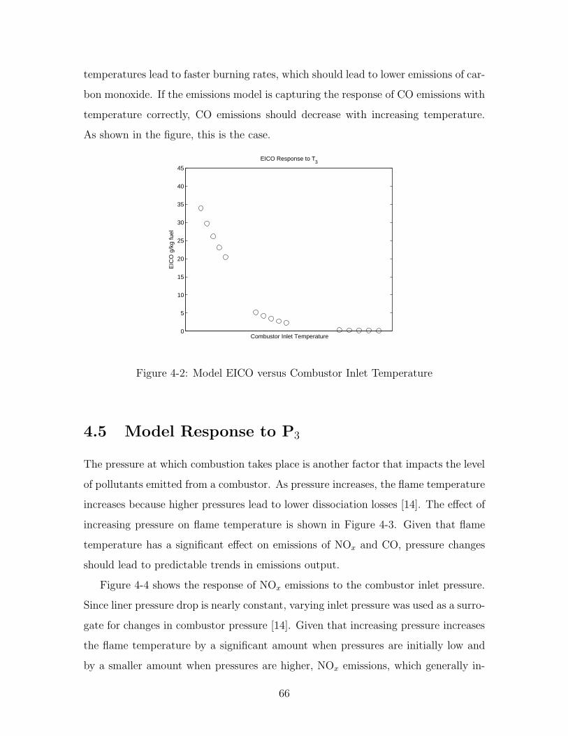
temperatures lead to faster burning rates, which should lead to lower emissions of car-
bon monoxide. If the emissions model is capturing the response of CO emissions with
temperature correctly, CO emissions should decrease with increasing temperature.
As shown in the figure, this is the case.
0
5
10
15
20
25
30
35
40
45
EICO Response to T3
Combustor Inlet Temperature
EIC
O g
/kg
fuel
Figure 4-2: Model EICO versus Combustor Inlet Temperature
4.5 Model Response to P3
The pressure at which combustion takes place is another factor that impacts the level
of pollutants emitted from a combustor. As pressure increases, the flame temperature
increases because higher pressures lead to lower dissociation losses [14]. The effect of
increasing pressure on flame temperature is shown in Figure 4-3. Given that flame
temperature has a significant effect on emissions of NOx and CO, pressure changes
should lead to predictable trends in emissions output.
Figure 4-4 shows the response of NOx emissions to the combustor inlet pressure.
Since liner pressure drop is nearly constant, varying inlet pressure was used as a surro-
gate for changes in combustor pressure [14]. Given that increasing pressure increases
the flame temperature by a significant amount when pressures are initially low and
by a smaller amount when pressures are higher, NOx emissions, which generally in-
66

5 10 15 20 252200
2300
2400
2500
2600
2700
2800
2900
3000
Pressure, atm
Fla
me
Tem
pera
ture
, K
Figure 4-3: Effect of Pressure on Flame Temperature, adapted from [14]
0
2
4
6
8
10
12
14
16
18
EINOx Response to P
3
Combustor Inlet Pressure
EIN
Ox g
/kg
fuel
Figure 4-4: Model EINOx versus Combustor Inlet Pressure
crease with flame temperature, should show increases at all engine conditions, with
the lower power conditions responding more strongly to pressure. Figure 4-4 shows
that the model is capturing this response.
Figure 4-5 gives the response of the model CO emissions to increasing pressure.
Since CO emissions generally decrease with flame temperature, pressure increases
should lead to decreasing CO emissions. The effect should be more pronounced at
67
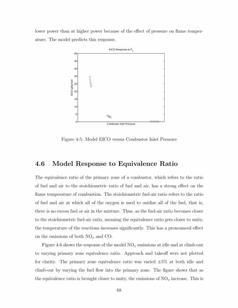
lower power than at higher power because of the effect of pressure on flame temper-
ature. The model predicts this response.
0
5
10
15
20
25
30
35
40
45
EICO Response to P3
Combustor Inlet Pressure
EIC
O g
/kg
fuel
Figure 4-5: Model EICO versus Combustor Inlet Pressure
4.6 Model Response to Equivalence Ratio
The equivalence ratio of the primary zone of a combustor, which refers to the ratio
of fuel and air to the stoichiometric ratio of fuel and air, has a strong effect on the
flame temperature of combustion. The stoichiometric fuel-air ratio refers to the ratio
of fuel and air at which all of the oxygen is used to oxidize all of the fuel, that is,
there is no excess fuel or air in the mixture. Thus, as the fuel-air ratio becomes closer
to the stoichiometric fuel-air ratio, meaning the equivalence ratio gets closer to unity,
the temperature of the reactions increases significantly. This has a pronounced effect
on the emissions of both NOx and CO.
Figure 4-6 shows the response of the model NOx emissions at idle and at climb-out
to varying primary zone equivalence ratio. Approach and takeoff were not plotted
for clarity. The primary zone equivalence ratio was varied ±5% at both idle and
climb-out by varying the fuel flow into the primary zone. The figure shows that as
the equivalence ratio is brought closer to unity, the emissions of NOx increase. This is
68

the appropriate result since the flame temperature increases as the equivalence ratio
moves closer to unity.
10
2
4
6
8
10
12
14
16
18
EINOx Response to Primary Zone Equivalence Ratio
Primary Zone Equivalence Ratio
EIN
Ox g
/kg
fuel
Figure 4-6: Model EINOx versus Primary Zone Equivalence Ratio
Figure 4-7 gives the response of the model CO emissions at idle and climb to
varying primary zone equivalence ratio. The results were produced in the same way
as they were for Figure 4-6. At the idle condition, where large amounts of CO are
anticipated, the effect of increasing equivalence ratio has a significant impact on CO
emissions. The increasing flame temperatures caused by increasing the equivalence
ratio causes a reduction in CO emissions. The climb-out condition reveals a weaker
response of CO to increasing equivalence ratio. At this condition, the temperatures
are high and the varying equivalence ratio does not reduce the temperature enough
to have a significant impact on CO. This is consistent with what the model should
be estimating.
69

10
10
20
30
40
50
60
70EICO Response to Primary Zone Equivalence Ratio
Primary Zone Equivalence Ratio
EIC
O g
/kg
fuel
Figure 4-7: Model EICO versus Primary Zone Equivalence Ratio
4.7 Capturing the Effects of Gas Turbine Combus-
tor Design
Most of the discussion thus far regarding the response of NOx and CO emissions has
been based on the correct modeling of the chemical processes taking place within the
combustor. The physics-based emissions model however, must also account for the
physical layout of a gas turbine combustor and how that affects the combustion that
takes place. To determine if the model is capturing the physics and chemistry along
the length of the combustor, the emissions output from each zone was studied for
each ICAO LTO-cycle power setting.
4.7.1 Idle Emissions Output
Figure 4-8 shows the NOx and CO emissions in grams that are produced or oxidized
in each zone of the model of an industry combustor at the idle power setting. For
NOx, nearly all of the production occurs in the primary zone of the combustor as
anticipated given that the temperatures are highest in the primary zone, and that
at idle power, the temperature is quickly reduced below the value of about 1800
70
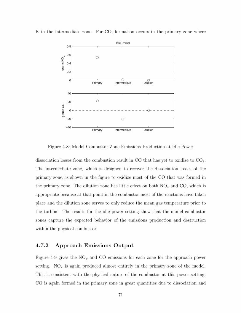
K in the intermediate zone. For CO, formation occurs in the primary zone where
Primary Intermediate Dilution0
0.2
0.4
0.6
0.8
gram
s N
Ox
Idle Power
Primary Intermediate Dilution−40
−20
0
20
40
gram
s C
O
Figure 4-8: Model Combustor Zone Emissions Production at Idle Power
dissociation losses from the combustion result in CO that has yet to oxidize to CO2.
The intermediate zone, which is designed to recover the dissociation losses of the
primary zone, is shown in the figure to oxidize most of the CO that was formed in
the primary zone. The dilution zone has little effect on both NOx and CO, which is
appropriate because at that point in the combustor most of the reactions have taken
place and the dilution zone serves to only reduce the mean gas temperature prior to
the turbine. The results for the idle power setting show that the model combustor
zones capture the expected behavior of the emissions production and destruction
within the physical combustor.
4.7.2 Approach Emissions Output
Figure 4-9 gives the NOx and CO emissions for each zone for the approach power
setting. NOx is again produced almost entirely in the primary zone of the model.
This is consistent with the physical nature of the combustor at this power setting.
CO is again formed in the primary zone in great quantities due to dissociation and
71

Primary Intermediate Dilution0
0.5
1
1.5
2
gram
s N
Ox
Approach Power
Primary Intermediate Dilution−200
−100
0
100
200
gram
s C
O
Figure 4-9: Model Combustor Zone Emissions Production at Approach Power
oxidized in the intermediate zone. The dilution zone is again having little effect on
the emissions outputs. The approach condition reveals that the CO formed in the
primary zone is greater than that formed in the primary zone at the idle condition.
This is consistent with CO kinetics. As shown in Figure 4-10, at low equivalence
ratios, CO oxidation does not reach the equilibrium value of CO. As equivalence
ratio is increased however, CO levels approach equilibrium in the primary zone. For
the range of equivalence ratios typically found in the primary zone of a gas turbine
combustor, (about 0.6 to 1.8), the non-equilibrium CO values can be lower than CO
levels at higher equivalence ratios where CO is at its equilibrium value. This is the
case for the equivalence ratios of the industry combustor at idle and approach. Thus,
even though the CO emissions from gas turbine combustors are higher at idle than
they are at higher power settings, the CO emissions from the primary zone of the
combustor are lower at idle in some cases than at higher power. The model estimates
this correctly.
72

Figure 4-10: Carbon Monoxide Emissions versus Primary Zone Equivalence Ratio[14]
4.7.3 Climb-Out Emissions Output
The results of the climb-out power setting emissions outputs from each zone of the
model were similar to those of the idle and approach settings and are shown in Figure
4-11. The NOx emissions are mainly from the primary zone, though the intermediate
zone is shown to be producing some NOx. This is due to the higher temperature
conditions at this power setting and is an appropriate result. The CO emissions
follow the same trend as they did for the other power settings. CO is formed in the
primary zone and oxidized in the intermediate zone. The CO is again attaining an
equilibrium value in the primary zone that is higher than that of the approach setting.
This is consistent with Figure 4-10 given that the climb-out condition has a higher
primary zone equivalence ratio than the approach condition.
4.7.4 Takeoff Emissions Output
The takeoff results are also similar to the other power settings and are shown in Figure
4-12. The intermediate NOx production is higher still at takeoff, which is consistent
with the fact that the temperatures are highest at this condition and the interme-
73
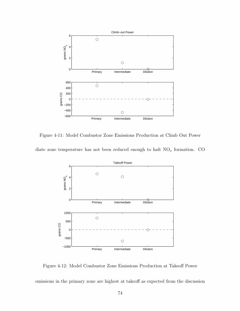
Primary Intermediate Dilution0
2
4
6
gram
s N
Ox
Climb−out Power
Primary Intermediate Dilution−600
−400
−200
0
200
400
600
gram
s C
O
Figure 4-11: Model Combustor Zone Emissions Production at Climb Out Power
diate zone temperature has not been reduced enough to halt NOx formation. CO
Primary Intermediate Dilution0
2
4
6
gram
s N
Ox
Takeoff Power
Primary Intermediate Dilution−1000
−500
0
500
1000
gram
s C
O
Figure 4-12: Model Combustor Zone Emissions Production at Takeoff Power
emissions in the primary zone are highest at takeoff as expected from the discussion
74
on equivalence ratio and CO equilibrium.
4.7.5 Assessment of Model Capability
The model was shown to correctly capture trends in emissions outputs. The responses
to temperature, pressure and equivalence ratio were appropriate and the production
and oxidation of emissions within the various zones of the model match those expected
for an example industry combustor. Confidence in the model’s ability to represent the
physical relationships between operating conditions, design parameters, and pollutant
emissions in a consistent manner has thus been established.
75

76
Chapter 5
Results
This chapter presents results generated by the model using industry data for the
five combustors discussed previously. The results include emissions estimates from
the model for Engines 1, 2, and 3, the model estimates of the effects of the design
changes from Engine 1 to Engine 1a and Engine 3 to Engine 3a. Also included is a
model estimate of NOx and CO emissions for a full throttle sweep of Engine 1a. The
results are all discussed in the context of the objectives of the model as described in
sections 1.4 and 2.1.
5.1 Model Predictions for Engines 1, 2, and 3
Using the individually set unmixedness curve fit for Engines 1, 2, and 3, the model was
run using the input data for the four ICAO LTO-cycle points and the predictions for
NOx and CO were compared to the ICAO certification data. The NOx predictions are
also compared to predictions from the NPSS single-annular combustor NOx empirical
model given in Equation 1.4, to determine how well the model performs relative to
an empirical model at predicting trends in the emission levels of different combustor
designs.
77

5.1.1 Overview of the Results
The use of the model to predict the emissions of NOx and CO from Engines 1, 2, and
3 revealed that the NOx estimates from the model were better than the estimates
from the empirical model for most cases, with the exception of the idle condition for
each engine, which was predicted poorly by both the physics-based model and the
empirical model. For CO emissions, the physics-based model estimates idle CO, which
is the dominant contribution to CO Dp/Foo, within the uncertainty bounds for all
three engines. At higher power the model does not perform as well, estimating most
of the approach, climb-out, and takeoff CO levels outside of the uncertainty bounds.
For all three engines however, the CO Dp/Foo is estimated within the uncertainty
bounds, owing to the dominance of idle CO and the model’s ability to estimate it
within the uncertainty in the data for these engines.
5.1.2 Engine 1 Estimates
The results of the model estimates for Engine 1 are shown in Figure 5-1. Figure 5-1a
is a comparison of the model estimated EINOx with the ICAO certification data and
the empirical model estimate. The whiskers on the ICAO data points cover the ±16%
uncertainty in the certification data. For Engine 1, the physics-based model estimates
the NOx emissions at approach, climb-out, and takeoff better than the empirical
model. Neither the physics-based model nor the empirical model estimate idle NOx
well. Figure 5-1b, is a comparison of the model estimated EICO with the ICAO
certification data. The whiskers on the ICAO points are the ±23% uncertainty in
the EICO certification data. There is no comparison to an empirical model because,
as mentioned previously, there are no non-proprietary empirical CO models. The
figure shows that the model estimates the emissions of CO from Engine 1 within the
uncertainty in the ICAO certification data for both idle and approach. Takeoff and
climb-out CO estimates for Engine 1 are outside of the uncertainty in the data, which
is unclear from the figure due to the low EICO values at those conditions. Figure 5-1c,
is a comparison of the model estimated Dp/Foo for NOx with the ICAO certification
78

value as well as the empirically estimated value, and the model estimated Dp/Foo for
CO with the ICAO certification value. The whiskers are again the uncertainty in the
NOx and CO ICAO certification data. The figure shows that the model estimates
both the NOx and CO Dp/Foo from Engine 1 within the uncertainty bounds. The
figure also shows that the empirical model estimated the NOx Dp/Foo within the
uncertainty bounds.
Idle Approach Climb Out Takeoff0
5
10
15
20
25
30
Comparison of ICAO Measured EINOx, Model Predicted EINO
x, and Empirical EINO
x
EIN
Ox g
/kg
fuel
ICAOModelEmpirical
(a) EINOx
Idle Approach Climb Out Takeoff0
5
10
15
20
25
30
35Comparison of ICAO Measured EICO and Model Predicted EICO
EIC
O g
/kg
fuel
ICAOModel
(b) EICO
NOx CO0
10
20
30
40
50
60
70
80
Comparison of ICAO NOx and CO Dp/Foo with Model Predicted NO
x and CO Dp/Foo
Dp/
Foo
g/k
N
ICAOModelEmpirical
(c) Dp/Foo
Figure 5-1: Emissions Estimates for Engine 1
79

5.1.3 Engine 2 Estimates
The results of the model estimates for Engine 2 are shown in Figure 5-2. The plots
give the EINOx, EICO, and Dp/Foo estimates of the model compared to the ICAO
certification data and the empirical model estimates where applicable. The physics-
based model estimates the NOx emissions at approach, climb-out, and takeoff within
the ICAO uncertainty in the data and does a poor job estimating the NOx at idle. The
empirical model estimates the climb-out condition within the uncertainty in the data
but not the idle, approach, or takeoff condition. The EICO model estimate for Engine
2, shown in Figure 5-2b, is within the uncertainty in the data at the idle condition
and outside of the uncertainty in the data at approach, climb-out, and takeoff. The
Dp/Foo estimate for NOx, shown in Figure 5-2c, is outside of the uncertainty band
for both the physics-based model and the empirical model. The Dp/Foo estimate for
CO, also shown in Figure 5-2c, is within the uncertainty in the CO certification data.
5.1.4 Engine 3 Estimates
The results for Engine 3 are shown in Figure 5-3. The plots are for EINOx, EICO,
and Dp/Foo for NOx and CO, as they were in Figures 5-1 and 5-2. Figure 5-3a, shows
that the model is estimating NOx emissions within the uncertainty bounds at climb-
out and takeoff and is not predicting NOx emissions within the uncertainty in the
data at idle and approach. The same is true for the estimates from the empirical NOx
model. Figure 5-3b, shows that estimate of idle EICO is within the uncertainty in the
data but the approach EICO estimate is not. The climb-out and takeoff conditions
are also estimated outside of the uncertainty bounds, which is not shown clearly in
the figure. The Dp/Foo estimates for NOx and CO are shown in Figure 5-3c. The
model estimates both the NOx and CO Dp/Foo within the uncertainty bounds. The
empirical NOx model also estimates the Dp/Foo for NOx within the uncertainty in
the data.
80
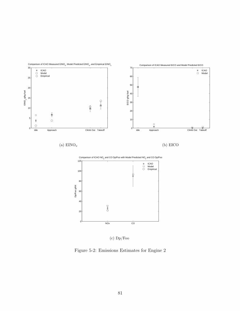
Idle Approach Climb Out Takeoff0
5
10
15
20
25
30
Comparison of ICAO Measured EINOx, Model Predicted EINO
x, and Empirical EINO
x
EIN
Ox g
/kg
fuel
ICAOModelEmpirical
(a) EINOx
Idle Approach Climb Out Takeoff0
10
20
30
40
50
60
70Comparison of ICAO Measured EICO and Model Predicted EICO
EIC
O g
/kg
fuel
ICAOModel
(b) EICO
NOx CO0
20
40
60
80
100
120
Comparison of ICAO NOx and CO Dp/Foo with Model Predicted NO
x and CO Dp/Foo
Dp/
Foo
g/k
N
ICAOModelEmpirical
(c) Dp/Foo
Figure 5-2: Emissions Estimates for Engine 2
81

Idle Approach Climb Out Takeoff0
5
10
15
20
25
30
Comparison of ICAO Measured EINOx, Model Predicted EINO
x, and Empirical EINO
x
EIN
Ox g
/kg
fuel
ICAOModelEmpirical
(a) EINOx
Idle Approach Climb Out Takeoff0
10
20
30
40
50
60
70
80Comparison of ICAO Measured EICO and Model Predicted EICO
EIC
O g
/kg
fuel
ICAOModel
(b) EICO
NOx CO0
20
40
60
80
100
120
Comparison of ICAO NOx and CO Dp/Foo with Model Predicted NO
x and CO Dp/Foo
Dp/
Foo
g/k
N
ICAOModelEmpirical
(c) Dp/Foo
Figure 5-3: Emissions Estimates for Engine 3
82

5.1.5 Overall Estimates
Figure 5-4 shows the estimates from the model of EINOx and EICO for all three
engines. The figure also includes the empirical NOx model estimates for all three
engines. The solid line is the line of exact match between the estimated and the
certification data emissions of NOx and CO. The dashed lines are the uncertainty
bounds for each emission. The plus marks on the figure are the model estimated
NOx and CO values and the circles are the empirical model estimated NOx values.
The figure shows that the estimated NOx emissions from the model are closer to the
0 5 10 15 20 25 300
5
10
15
20
25
30
Comparison of ICAO Measured EINOx and Model Predicted EINO
x
ICAO Certification EINOx g/kg fuel
Mod
el P
redi
cted
EIN
Ox g
/kg
fuel
(a) EINOx
0 10 20 30 40 50 60 70 800
10
20
30
40
50
60
70
80Comparison of ICAO Measured EICO and Model Predicted EICO
ICAO Certification EICO g/kg fuel
Mod
el P
redi
cted
EIC
O g
/kg
fuel
(b) EICO
Figure 5-4: Emissions Estimates for Engines 1, 2, and 3
ICAO certification data than the empirical model in most cases. The lower values
of EINOx (below 5 g/kg fuel on the figure), where both the model and the empirical
model are outside of the uncertainty bands, are the idle conditions where neither
model performs well. The figure also shows that the estimated CO emissions from
the model are within the uncertainty bands for the higher values of EICO, which
make the most significant contributions to CO Dp/Foo.
83

5.1.6 Discussion of Engine 1, 2, and 3 Model Estimates
From Figures 5-1, 5-2, 5-3, and 5-4, it is clear that the estimates of NOx emissions are
as good or better than those of the empirical model at nearly all conditions. The only
exception is the low power condition, where both the physics-based model and the
empirical model do a poor job. This is likely due to the complex NOx chemistry that
may not be modeled appropriately in the physics-based model at lower temperature
and due to the emphasis on the Zeldovich mechanism, which is not dominant at low
power, in the empirical model. For these three engines the model is thus meeting the
objective of performing as well as an empirical NOx model at predicting trends across
different engine designs and operating conditions.
The figures also show that the model estimates low power emissions of carbon
monoxide well, since all idle estimates were within the uncertainty bounds for CO.
The CO emissions at higher power levels are not estimated as well by the model but,
since these higher power conditions produce low emissions of CO relative to idle CO,
the Dp/Foo estimates are within the uncertainty in the data. For these three engines
the model is thus meeting the objective of predicting CO Dp/Foo levels within the
uncertainty in the data.
5.2 Predicting the Effects of Design Changes
An objective of physics-based emissions model is to predict broad trends in pollu-
tant emissions using a single methodology across different combustor designs and
operating conditions using only high-level parameters. The following results assess
the performance of the model in terms of meeting that objective through the model
estimates of the effects of two design changes on the emissions of NOx and CO.
5.2.1 Overview of Results
The results for both design changes were obtained by using the individually set un-
mixedness curves discussed in Chapter 3. For the design change from Engine 1a to
84

Engine 1, the emissions model performs better than the empirical model at estimating
individual levels of NOx at the four LTO-cycle points. The empirical model performs
better than the physics-based model at estimating the NOx Dp/Foo change between
the two engines, but this is due to error cancellations between the certification points
when they are summed in the Dp/Foo metric. The CO predictions from the model
are outside of the uncertainty in the data for most of the certification points for the
two engines, but the change in CO Dp/Foo from Engine 1a to Engine 1 is captured
correctly.
For the design change from Engine 3 to Engine 3a, the emissions model performs
as well as the empirical model in terms of NOx estimates. The CO estimates from
the model are outside of the uncertainty in the data for most conditions for Engines
3 and 3a, but the change in Dp/Foo between the two engines is captured within the
uncertainty in the data by the model.
5.2.2 Engine 1a to Engine 1
Table 5.1 compares the model estimated NOx emissions for Engine 1a with the ICAO
certification data and the empirically estimated NOx emissions at the four LTO-
cycle points. The model estimates of NOx are all within ±16% uncertainty with
ICAO Model EmpiricalEINOx g/kg fuel EINOx g/kg fuel EINOx g/kg fuel
Idle 4.43 1.40 1.53Approach 11.26 12.15 5.01Climb Out 14.30 14.15 18.32
Takeoff 19.19 19.58 24.19
Table 5.1: Engine 1a NOx Emissions
the exception of the idle setting. None of the empirical estimates are within the
uncertainty in the certification data. Table 5.2 compares the model estimated CO
emissions for Engine 1a with the ICAO certification data. The model estimates for
CO are all outside the ±23% uncertainty with the exception of approach, with the idle
CO being overestimated by 82%. Idle CO can be estimated within the uncertainty
85
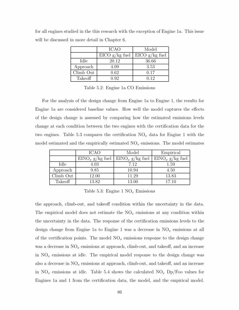
for all engines studied in the this research with the exception of Engine 1a. This issue
will be discussed in more detail in Chapter 6.
ICAO ModelEICO g/kg fuel EICO g/kg fuel
Idle 20.12 36.66Approach 4.09 3.53Climb Out 0.62 0.17
Takeoff 0.92 0.12
Table 5.2: Engine 1a CO Emissions
For the analysis of the design change from Engine 1a to Engine 1, the results for
Engine 1a are considered baseline values. How well the model captures the effects
of the design change is assessed by comparing how the estimated emissions levels
change at each condition between the two engines with the certification data for the
two engines. Table 5.3 compares the certification NOx data for Engine 1 with the
model estimated and the empirically estimated NOx emissions. The model estimates
ICAO Model EmpiricalEINOx g/kg fuel EINOx g/kg fuel EINOx g/kg fuel
Idle 4.03 7.12 1.59Approach 9.85 10.94 4.50Climb Out 12.00 11.29 13.83
Takeoff 13.82 13.00 17.10
Table 5.3: Engine 1 NOx Emissions
the approach, climb-out, and takeoff condition within the uncertainty in the data.
The empirical model does not estimate the NOx emissions at any condition within
the uncertainty in the data. The response of the certification emissions levels to the
design change from Engine 1a to Engine 1 was a decrease in NOx emissions at all
of the certification points. The model NOx emissions response to the design change
was a decrease in NOx emissions at approach, climb-out, and takeoff, and an increase
in NOx emissions at idle. The empirical model response to the design change was
also a decrease in NOx emissions at approach, climb-out, and takeoff, and an increase
in NOx emissions at idle. Table 5.4 shows the calculated NOx Dp/Foo values for
Engines 1a and 1 from the certification data, the model, and the empirical model.
86
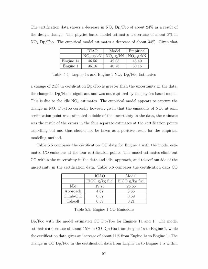
The certification data shows a decrease in NOx Dp/Foo of about 24% as a result of
the design change. The physics-based model estimates a decrease of about 3% in
NOx Dp/Foo. The empirical model estimates a decrease of about 34%. Given that
ICAO Model EmpiricalNOx g/kN NOx g/kN NOx g/kN
Engine 1a 46.56 42.08 45.49Engine 1 35.16 40.76 30.16
Table 5.4: Engine 1a and Engine 1 NOx Dp/Foo Estimates
a change of 24% in certification Dp/Foo is greater than the uncertainty in the data,
the change in Dp/Foo is signficant and was not captured by the physics-based model.
This is due to the idle NOx estimates. The empirical model appears to capture the
change in NOx Dp/Foo correctly however, given that the emissions of NOx at each
certification point was estimated outside of the uncertainty in the data, the estimate
was the result of the errors in the four separate estimates at the certification points
cancelling out and thus should not be taken as a positive result for the empirical
modeling method.
Table 5.5 compares the certification CO data for Engine 1 with the model esti-
mated CO emissions at the four certification points. The model estimates climb-out
CO within the uncertainty in the data and idle, approach, and takeoff outside of the
uncertainty in the certification data. Table 5.6 compares the certification data CO
ICAO ModelEICO g/kg fuel EICO g/kg fuel
Idle 19.73 26.66Approach 4.67 3.56Climb-Out 0.57 0.69
Takeoff 0.59 0.21
Table 5.5: Engine 1 CO Emissions
Dp/Foo with the model estimated CO Dp/Foo for Engines 1a and 1. The model
estimates a decrease of about 15% in CO Dp/Foo from Engine 1a to Engine 1, while
the certification data gives an increase of about 11% from Engine 1a to Engine 1. The
change in CO Dp/Foo in the certification data from Engine 1a to Engine 1 is within
87

the uncertainty in the data and therefore is not significant. The model estimate,
which is a change of less than 23%, is thus appropriate.
ICAO ModelCO g/kN CO g/kN
Engine 1a 38.52 65.10Engine 1 42.67 55.30
Table 5.6: Engine 1a and Engine 1 CO Dp/Foo Estimates
5.2.3 Discussion of the Engine 1a to Engine 1 Design Change
Results
One of the objectives of the model is to predict broad trends in emissions levels from
different combustor designs within the uncertainty in the certification data for CO
and as well as empirical models for NOx. The change in CO Dp/Foo was captured
correctly because there was no significant change in the certification data (meaning
the change was within the uncertainty in the data) and the model estimated this.
However, the model did not estimate the emissions levels of CO at the individual
certification points within the uncertainty in the data with the exception of climb-out
for Engine 1 using the Engine 1a derived unmixedness curve. The objective for CO
emissions prediction was therefore, not met for this design change but the results
are promising because the objective of predicting the correct sign for changes in CO
emission with changing design and operating parameters was met.
For NOx emissions, the model estimates the emissions levels within the uncertainty
in the data for all but the idle condition, but does not capture the magnitude of the
change in NOx Dp/Foo. The empirical model does not estimate the emissions levels
within the uncertainty in the data for any condition, but it does capture the change
in NOx Dp/Foo within the uncertainty in the data. However, this was the result of
error cancelling among the four certification points. The objective for NOx emissions
prediction therefore, was not met because the model did not perform as well as the
empirical model in terms of the NOx Dp/Foo, but given that the only weakness of
88

the model for NOx emissions appears to be predicting idle NOx, the results for NOx
are also promising.
Another objective of the model is to include high-level design parameters and
operating conditions that would be convienient for an expert to use in projecting
future technology. Figure 5-5 shows the percentage changes in the model inputs for
the design change from Engine 1 to Engine 1a. The inputs shown in the figure are
the only elements of the model that were changed between the two engines. Since the
results of the design change from Engine 1a to Engine 1 were promising both in terms
of NOx and CO, the possibility of creating a model using only high-level, convienient
parameters is plausible.
Idle Approach Climb Out Takeoff0
5
10
15
20
25Percentage Change in Engine 1a Input Parameters from Engine 1
%
air flowfuel flowP3T3Volume
Figure 5-5: Percentage Change of Inputs from Engine 1 to Engine 1a
5.2.4 Engine 3 to Engine 3a
Tables 5.7 and 5.8 show the model and empirical estimates of NOx emissions for
Engine 3 compared to the ICAO certification data and the model estimates of CO
emissions for Engine 3 compared to the ICAO certification data. The model NOx
estimates are within the uncertainty in the data for climb-out and takeoff and outside
of the uncertainty for idle and approach. The empirical model estimates are also
89
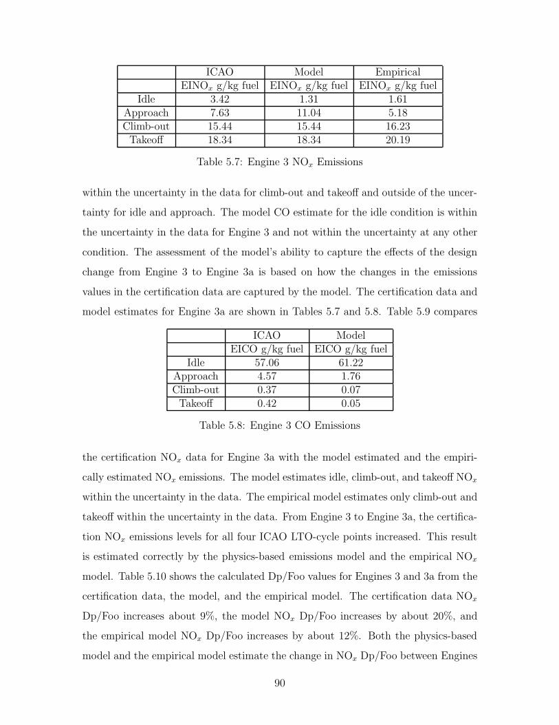
ICAO Model EmpiricalEINOx g/kg fuel EINOx g/kg fuel EINOx g/kg fuel
Idle 3.42 1.31 1.61Approach 7.63 11.04 5.18Climb-out 15.44 15.44 16.23Takeoff 18.34 18.34 20.19
Table 5.7: Engine 3 NOx Emissions
within the uncertainty in the data for climb-out and takeoff and outside of the uncer-
tainty for idle and approach. The model CO estimate for the idle condition is within
the uncertainty in the data for Engine 3 and not within the uncertainty at any other
condition. The assessment of the model’s ability to capture the effects of the design
change from Engine 3 to Engine 3a is based on how the changes in the emissions
values in the certification data are captured by the model. The certification data and
model estimates for Engine 3a are shown in Tables 5.7 and 5.8. Table 5.9 compares
ICAO ModelEICO g/kg fuel EICO g/kg fuel
Idle 57.06 61.22Approach 4.57 1.76Climb-out 0.37 0.07Takeoff 0.42 0.05
Table 5.8: Engine 3 CO Emissions
the certification NOx data for Engine 3a with the model estimated and the empiri-
cally estimated NOx emissions. The model estimates idle, climb-out, and takeoff NOx
within the uncertainty in the data. The empirical model estimates only climb-out and
takeoff within the uncertainty in the data. From Engine 3 to Engine 3a, the certifica-
tion NOx emissions levels for all four ICAO LTO-cycle points increased. This result
is estimated correctly by the physics-based emissions model and the empirical NOx
model. Table 5.10 shows the calculated Dp/Foo values for Engines 3 and 3a from the
certification data, the model, and the empirical model. The certification data NOx
Dp/Foo increases about 9%, the model NOx Dp/Foo increases by about 20%, and
the empirical model NOx Dp/Foo increases by about 12%. Both the physics-based
model and the empirical model estimate the change in NOx Dp/Foo between Engines
90

ICAO Model EmpiricalEINOx g/kg fuel EINOx g/kg fuel EINOx g/kg fuel
Idle 3.59 4.12 1.74Approach 8.02 11.23 5.59Climb-out 16.68 17.01 17.98Takeoff 20.40 19.28 22.68
Table 5.9: Engine 3a NOx Emissions
3 and 3a within the uncertainty in the certification data. Table 5.11 compares the
ICAO Model EmpiricalNOx g/kN NOx g/kN NOx g/kN
Engine 3 35.81 34.85 32.90Engine 3a 39.03 41.98 36.78
Table 5.10: Engine 3 and Engine 3a NOx Dp/Foo Estimates
certification CO data for Engine 3a with the model estimated CO emissions at the
four LTO-cycle points. The model does not estimate the CO emissions at any of
the four points within the uncertainty in the certification data. Table 5.12 compares
ICAO ModelEICO g/kg fuel EICO g/kg fuel
Idle 49.94 68.33Approach 3.68 0.80Climb-out 0.38 0.05Takeoff 0.52 0.06
Table 5.11: Engine 3a CO Emissions
the certification data CO Dp/Foo with the model estimated CO Dp/Foo for Engines
3 and 3a. The model estimates an increase of about 9% in CO Dp/Foo while the
certification data contains a decrease of about 14%. There is therefore a negligible
change in CO Dp/Foo given the uncertainty in the data, which is estimated correctly
by the model.
91

ICAO ModelCO g/kN CO g/kN
Engine 3 94.35 98.50Engine 3a 81.49 107.73
Table 5.12: Engine 3 and Engine 3a CO Dp/Foo Estimates
5.2.5 Discussion of the Engine 3 to Engine 3a Design Change
Results
The effect of the design change from Engine 3 to Engine 3a on NOx emissions is
captured by the physics-based model as well as or better than the empirical model for
all cases. The emissions model thus meets the objective of predicting NOx emissions
as well as an empirical model for this particular design change. The effect of the
design change on CO emissions is captured by the model within the uncertainty in
the data in terms of CO Dp/Foo, but the results are not as good for the individual
data points. The objective of predicting CO emissions within the uncertainty in the
data was therefore, not met for this particular design change, but the results were
again promising.
Figure 5-6 gives the percentage changes to the input parameters of the model from
Engine 3 to Engine 3a. Using only these parameter changes the model predicted NOx
Idle Approach Climb Out Takeoff0
5
10
15
20
25Percentage Change in Engine 3a Input Parameters from Engine 3
%
air flowfuel flowP3T3Volume
Figure 5-6: Percentage Change of Inputs from Engine 3 to Engine 3a
92

emissions better than the empirical model and CO Dp/Foo within the uncertainty
in the data, meeting the objective of using high-level, convienient design parameters
and operating conditions in the model.
5.3 NOx Estimates for a Full Throttle Sweep
To assess the model’s ability to consistently capture the effect of combustor operating
conditions on pollutant emissions, a full throttle sweep of operating conditions for
Engine 1a was run with the model and the results were compared to data collected
during the engine’s certification testing. To show the benefit of capturing the effects
of operating conditions on pollutant emissions, the model estimates for NOx and CO
are compared with the estimates from the Boeing fuel flow method 2 (BM2), which is
a widely used method for modeling emissions of NOx and CO at different operating
conditions [12].
5.3.1 Throttle Sweep Emissions Estimates
Figure 5-7 compares the emissions model estimates with the data collected on Engine
1a during certification testing for NOx and CO. The empirical NOx model results are
also shown. The figure shows that the NOx estimates of the model follow the trend
in the certification data more closely than the empirical model. The physics-based
emissions model is therefore capturing the relationship between operating conditions
and NOx emissions better than the empirical model.
The CO estimate from the model follows the same trend as the test CO data
but at low fuel flow rates the CO estimates from the model are significantly higher
than the test data values. The uncertainty is not shown on the plot but the CO
estimates at these low power conditions are not within the uncertainty in the data.
The physical relationship between CO emissions and operating conditions however is
captured because the trend is estimated correctly.
93
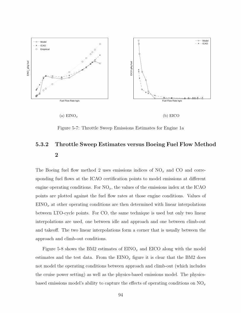
Fuel Flow Rate kg/s
EIN
Ox g
/kg
fuel
Model
ICAO
Empirical
(a) EINOx
Fuel Flow Rate kg/s
EIC
O g
/kg
fuel
ModelICAO
(b) EICO
Figure 5-7: Throttle Sweep Emissions Estimates for Engine 1a
5.3.2 Throttle Sweep Estimates versus Boeing Fuel Flow Method
2
The Boeing fuel flow method 2 uses emissions indices of NOx and CO and corre-
sponding fuel flows at the ICAO certification points to model emissions at different
engine operating conditions. For NOx, the values of the emissions index at the ICAO
points are plotted against the fuel flow rates at those engine conditions. Values of
EINOx at other operating conditions are then determined with linear interpolations
between LTO-cycle points. For CO, the same technique is used but only two linear
interpolations are used, one between idle and approach and one between climb-out
and takeoff. The two linear interpolations form a corner that is usually between the
approach and climb-out conditions.
Figure 5-8 shows the BM2 estimates of EINOx and EICO along with the model
estimates and the test data. From the EINOx figure it is clear that the BM2 does
not model the operating conditions between approach and climb-out (which includes
the cruise power setting) as well as the physics-based emissions model. The physics-
based emissions model’s ability to capture the effects of operating conditions on NOx
94

emissions makes it a more suitable model in this case for estimating the impact
of aircraft operations than the BM2. The EICO figure shows that the physics-based
emissions model and the BM2 both estimate the correct trend of EICO with increasing
fuel flow rate.
Fuel Flow Rate kg/s
EIN
Ox g
/kg
fuel
Model
ICAO
BM2
(a) EINOx
Fuel Flow Rate kg/s
EIC
O g
/kg
fuel
ModelICAOBM2
(b) EICO
Figure 5-8: Throttle Sweep Emissions Estimates for Engine 1a Compared with BoeingFuel Flow Method 2
95

96

Chapter 6
Conclusions and Future Work
6.1 Conclusions
The objective of this thesis was to create a physics-based emissions model for predict-
ing emissions of potential future gas turbine combustors within quantified uncertainty
bounds. To make a successful emissions model for a policy making tool, the model
was required to capture the physical relationships among operating conditions, sim-
plified combustor design parameters, and pollutant emissions in a consistent way with
one modeling methodology. It was desired first that the model predict the correct
sign for changes in emissions with changes in design and operating conditions and if
successful, to then predict changes in emissions with changes in design and operating
conditions with an accuracy that approaches that of the uncertainty and variability
of measurements of emissions indices for the active fleet. The model presented in this
thesis did not meet all of the objectives but several important contributions to NOx
and CO emissions modeling were made.
NOx Emissions
The success criteria for predicting NOx emissions with the physics-based emissions
model was to estimate NOx emissions within the uncertainty in the certification data
or as well as an established empirical model if neither model estimates the emissions
levels within the certification data uncertainty. If the physics-based emissions model
97

could make estimates within the uncertainty in the data or as well as an empirical
model while using high-level physical parameters that may be used to project future
technologies, then the physics-based model would make a significant contribution to
emissions modeling for a policy-making tool.
The result of this work was the creation of a physics-based emissions model that
estimated NOx emissions as well as, or better than, the empirical model at all four
certification points for all of the engines and design changes studied in this thesis.
The model has the ability to consistently capture the relationships between operating
conditions and NOx emissions as shown in the throttle sweep analysis, and the model
has the ability to consistently capture the relationships between combustor design
parameters and NOx emissions as shown by the estimates for Engines 1, 2, and 3.
The ability to use one methodology to estimate broad trends in combustor designs
for NOx emissions across engine manufacturers was not studied since only one engine
manufacturer was engaged in this research. However, the model was shown to have
the ability to use one methodolgy to estimate broad trends in combustor designs
within a single engine family as shown by the design change analyses for Engines 1a
and 1 and Engines 3 and 3a. The model was also shown to perform better than BM2
for interpolating between certification points.
The only concern regarding the physics-based emissions model’s NOx emissions
estimates is that the model does not estimate low power emissions well. The estimates
for these cases were usually outside of the uncertainty in the data and the result was
that the Dp/Foo estimates for NOx emissions were not as good as the empirical
model estimates for some cases. The empirical model also did a poor job estimating
low power NOx emissions but the errors in emissions estimates at the four certification
points for the empirical model often cancelled out when the Dp/Foo was calculated.
Though the model did not strictly meet the objective of predicting NOx emissions
as well as an empirical model, the model did perform better than the empirical model.
The inability to correctly capture the change in NOx Dp/Foo for the two design
changes studied in this thesis was due only to poor idle NOx estimates. The physics-
based model has the ability to predict the emissions of a single annular gas turbine
98
combustor at specific operating conditions using high-level parameters as well as, and
in most cases better than, an empirical model. This is a significant contribution to
NOx emissions modeling capability.
CO Emissions
The success criteria for predicting CO emissions with the physics-based emissions
model was to estimate CO emissions within the uncertainty in the ICAO certification
data. There were no non-proprietary CO emissions models to use to compare how well
the model estimates CO emissions to other techniques, so using the uncertainty in the
certification data was the only means of assessing the models predictive capability.
Because there were no CO emissions models to compare the physics-based emissions
model estimates to, the ability to capture the relationships between operating con-
ditions, combustor design parameters, and pollutant emissions consistently, meaning
the ability to predict the correct trends in CO emissions with changing conditions
and design parameters, would be a significant contribution, even if the model could
not estimate the emissions of CO within the uncertainty in the data.
The results presented in this work show that the physical relationships among
operating conditions, high-level design parameters, and CO emissions are captured
correctly. The response of CO to design parameters like temperature and pressure, as
shown in Chapter 4, is captured correctly. The response of CO to changing operating
conditions, as shown in the full throttle sweep analysis of Engine 1a, is captured
correctly. The changes in CO Dp/Foo that resulted from the design changes from
Engine 1a to 1 and Engine 3 to 3a were captured within the uncertainty in the
certification data by the model. For most cases, the low power CO emissions, which
are more significant than the high power CO emissions because of their contributions
to the Dp/Foo, were estimated within the uncertainty in the data.
A concern regarding the CO emissions estimates from the physics-based model
is that for Engine 1a, the model did not estimate idle CO within the uncertainty in
the certification data. This led to an esitmate of the idle CO for Engine 1 outside
of the uncertainty in the data when the design change from Engine 1a to Engine 1
99

was studied. The result was that the CO estimates of the Dp/Foo values for each
engine were not within the uncertainty in the data, which means that the objective
of predicting CO emissions within the uncertainty was not met. The poor result
may have been the result of an incomplete intermediate zone model for CO emissions
predictions and should be looked at in more detail in the future.
Though the model did not meet all the objectives for CO emissions prediction
accuracy, it did meet the objective of capturing the physical relationships among
operating conditions, design parameters, and CO emissions. A non-proprietary CO
emissions model now exists as a result of this work, which is a significant contribution
to CO emissions modeling capability.
6.2 Future Work
Although this thesis made contributions to NOx and CO emissions modeling for
policy-making tools, the work is not done. There are several issues that should be
explored further. These are the inability to predict CO emissions within the uncer-
tainty in the data for Engine 1a, the poor low power NOx predictions, the extension
of the model to other combustor designs and manufacturing companies, and the de-
velopement of an addition to the model to enable the prediction of soot formation.
For CO emissions, different reactor arrangements, particularly for the intermediate
zone should be studied. For low power NOx emissions, different kinetic mechanisms
should be studied to determine whether or not poorly modeled low temperature NOx
chemistry is the cause of the erroneous predictions at low power.
If the objectives of this thesis can be met by modifying the reactor arrangement
and the kinetic mechanism, then the application of the model to other engine lines
and engine manufacturers should be studied. The physics-based emissions model
presented in this thesis was designed for single annular combustors and tested with
data from one engine manufacturer and one engine line. If the model is to be used in a
policy making tool it must be tested across engine manufacturers and across all power
levels. New models should also be created, using the same methods developed in this
100

thesis, for more advanced combustor layouts such as dual-annular combustors, rich-
quench-lean combustors, and lean-premix-prevaporize combustors, so that a broader
range of potential future technologies may be captured.
101

102
Bibliography
[1] The Boeing Company, “Boeing Current Market Outlook 2005,”
http://www.boeing.com/comerical/cmo.
[2] P.D. Norman, D.H. Lister, M. Lecht, P. Madden, K. Park, O. Penanhoat, C.
Plaisance, K. Renger, “Development of the technical basis for a New Emissions
Parameter covering teh whole AIRcraft operation: NEPAIR, Final Technical Re-
port,” CAEP/6-IP/17 Appendix B.
[3] J.J. Lee, S.P. Lukachko, I.A. Waitz, A. Schafer, “Historical and Future Trends in
Aircraft Performance, Cost, and Emissions,” Annu. Rev. Energy Environ. 2001,
26:167-200.
[4] N.E. Antoine, I.M. Kroo, “Aircraft Optimization for Minimal Environmental Im-
pact,” AIAA 2002-5667.
[5] H. Mongia and W. Dodds, “Low Emissions Propulsion Engine Combustor Tech-
nology Evolution Past, Present and Future,” GE Aircraft Engines, Cincinnati,
Ohio, U.S.A.
[6] Personal Communication with Professor Ian Waitz, MIT, March 2006.
[7] U.S. EPA, “Evalutation of Air Pollutant Emissions from Subsonic Commericial
Jet Aircraft,” EPA 420-R-99-013 April 1999.
[8] P.J. Jeanniot, “Environmental Review,” International Air Transport Associa-
tion, ISBN 92-9035-732-0.
103

[9] Intergovernmental Panel on Climate Change, Aviation and the Global Atmosphere,
Cambridge University Press, 1999.
[10] J.E. Green, “Greener by Design: The Technology Challenge,” The report by
the Technology Sub Group, Aero Journal, February 2002.
[11] Numerical Propulsion System Simulation tool, NASA Glenn.
[12] Baughcumb, S. L., S. C. Henderson, and T. G. Tritz. “Scheduled Civil Aircraft
Emission Inventories for 1976 and 1984: Database Development and Analysis,”
NASA CR-4722, 1996.
[13] A.M. Mellor and R.M. Washam, “Characteristic Time Correlations of Pollutant
Emissions from an Annular Gas Turbine Combustor,” Journal of Energy, Vol.
3, No. 4, Article 79-4135, July-August 1979.
[14] A.W. Lefebvre, Gas Turbine Combustion, McGraw-Hill 1983.
[15] M.G. Turner, A. Norris, J.P. Veres, “High Fidelity 3D Simulation of the GE90,”
AIAA 2003-3996.
[16] Gregory P. Smith, David M. Golden, Michael Frenklach, Nigel W. Moriarty, Boris
Eiteneer, Mikhail Goldenberg, C. Thomas Bowman, Ronald K. Hanson, Soonho
Song, William C. Gardiner, Jr., Vitali V. Lissianski, and Zhiwei Qin, “GRI mech
3.0,” http://www.me.berkeley.edu/gri-mech/.
[17] Stephen R. Turns, An Introduction to Combustion: concepts and applications,
The McGraw-Hill Companies, Inc. 2000.
[18] A. Ghoniem, Combustion Fundamentals and Applications, Course Notes,
Ghoniem 2005.
[19] G.J. Sturgess, J. Zelina, D.T. Shouse, W.M. Roquemore, “Emissions Reduction
Technologies for Military Gas Turbine Engines,” Journal of Propulsion and
Power, Vol. 21, No.2, March-April 2005.
104

[20] J.J. Lee, “Modeling Aviation’s Global Emissions, Uncertainty Analysis, and Ap-
plications to Policy,” PhD Thesis, Massachusetts Institute of Technology, 2004.
[21] Personal communication with Dr. Frank Lastrina, GEAE, 2005.
[22] J.B. Moss, Gas Turbine Pollutant Emissions: Predictive methods for gas turbine
combustor emissions, IMECHE Seminar Publications 2001.
[23] E.M. Greitzer, C.S. Tan, M.B. Graf, Internal Flow: Concepts and Applications,
Cambridge University Press 2004.
[24] N.K. Rizk, J.S. Chin, A.W. Marshall, M.K. Razdan, “Predictions of NOx For-
mation Under Combined Droplet and Partially Premixed Reaction of Diffusion
Flame Combustors,” Journal of Engineering for Gas Turbines and Power, Jan-
uary 2002, Vol. 124.
[25] C.J. Mordaunt, Combustion Instability in Land Based Gas Turbines,
www.personal.psu.edu/faculty/c/x/cxm283/research/GTI/stoichiometric combustor.jpg.
[26] Personal Communication with Nan-Suey Liu, NASA Glenn, April 2006.
[27] G.J. Sturgess, “An Account of FuelAir Unmixedness Effects on NOx Generation
in Gas Turbine Combustors,” IECEC-98-353, August 1998.
[28] C.K. Westbrook and F.L. Dryer, “Simplified Reaction Mechanisms for the Oxi-
dation of Hydrocarbon Fuels in Flames,” Combustion Science and Technology,
Vol. 27, 1981.
105
Related Documents


