A photoelastic investigation of three-dimensional contact stresses by Douglas Craig Schafer A thesis submitted to the Graduate Faculty in partial fulfillment of the requirements for the degree of MASTER OF SCIENCE in Mechanical Engineering Montana State University © Copyright by Douglas Craig Schafer (1968) Abstract: The object of this investigation was to produce an accurate analysis of the contact stress distribution on a three-dimensional body. The case presented in this thesis was a photoelastic study of an elastic body with surface discontinuities, loaded between rigid planes. A model, shaped similar to a roller bearing, was machined from an epoxy resin and loaded under a constant weight. The "frozen stress" method was then used in an analysis of the strains (stress) in the body and in the contact region in particular. Contact stresses were calculated using a Fortran program of the shear-difference equations and source data obtained from photographs of the photoelastic stress patterns in model slices. The results of this investigation were compared with theoretical predictions of contact stresses for a two-dimensional body of similar shape. The two-dimensional theory predicted higher contact stresses in the regions of discontinuities than were found actually to occur in the three-dimensional body.

Welcome message from author
This document is posted to help you gain knowledge. Please leave a comment to let me know what you think about it! Share it to your friends and learn new things together.
Transcript

A photoelastic investigation of three-dimensional contact stressesby Douglas Craig Schafer
A thesis submitted to the Graduate Faculty in partial fulfillment of the requirements for the degree ofMASTER OF SCIENCE in Mechanical EngineeringMontana State University© Copyright by Douglas Craig Schafer (1968)
Abstract:The object of this investigation was to produce an accurate analysis of the contact stress distribution ona three-dimensional body. The case presented in this thesis was a photoelastic study of an elastic bodywith surface discontinuities, loaded between rigid planes.
A model, shaped similar to a roller bearing, was machined from an epoxy resin and loaded under aconstant weight. The "frozen stress" method was then used in an analysis of the strains (stress) in thebody and in the contact region in particular. Contact stresses were calculated using a Fortran programof the shear-difference equations and source data obtained from photographs of the photoelastic stresspatterns in model slices.
The results of this investigation were compared with theoretical predictions of contact stresses for atwo-dimensional body of similar shape. The two-dimensional theory predicted higher contact stressesin the regions of discontinuities than were found actually to occur in the three-dimensional body.
A PHOTOELASTIC INVESTIGATION OF THREE-DIMENSIONAL CONTACT STRESSES
by
DOUGLAS CRAIG SCHAFER
A thesis submitted to the Graduate Faculty in partial fulfillment of the requirements for the degree
of
MASTER OF SCIENCE
in
Mechanical Engineering
Approved:
Head, Major Department
AChairman, Examining Committee
. ______DefagyGraduate DivyyzOn
MONTANA STATE UNIVERSITY Bozeman, Montana
March 1968
-iii-
Acknowledgments
The author would like, to express appreciation for the help
given by Dr. D. 0. Blackketter in this investigation.'
-iv-
Page
I. Introduction and Problem Statement _ _ _ _ _ _ _ _ _ i
2.1 An Outline of the. Frozen Stress Method _ _ _ _ _ _ _ 4
2.2 Properties of Plastics _ _ _ _ _ _ _ _ _ _ _ _ _ _ _ 5
2=3. Requirements of a Frozen Stress Analysis _ _ _ _ _ _ 7
3.1 Model Configuration- ̂ _ 3
3.2 Selection of a Plastic g
3.3 Model Fabrication _ _ _ _ _ _ _ _ _ _ _ _ _ _ _ _ _ 103.4 Model Loading and Slicing 13
-
3.5 Recording Isoclinics and Isochromatics _ _ _ _ _ _ _ 15
3.6 „ Equipment _ 20
4.1 Shear-Difference Equations _ _ _ _ _ _ _ _ _ _ _ _ _ _ 22
4.2 Sample Computation _ _ _ _ _ _ _ _ _ _ _ _ _ _ _ _ _ 29
5.1 A comparison of Experimental Results with aTwo-Dimensional Analytical Solution _ _ _ _ _ _ _ _ _ 34-
Table of Contents'
Appendix 44
List of Figures
Page
Figure. (I) Model Loading - - - - - - - - - - - - - - - - - - 9
Figure (2). Model Dimensions . - _ _ _ _ _ _ _ _ _ _ _ _ _ _ _ 11
Figure (3) Loading Frames and Annealing Oven 14-
Figure (4) Polariscope and Slicing Method _ _ _ _ _ _ _ _ _ 16
Figure (5) - Slicing Plan 18
Figure (6) Subslice No. 3 - - - - - - - - - - - - - - - - - - 23
Figure •(?) Surface Element _ _ _ _ _ _ _ _ _ _ _ _ _ _ _ _ 27
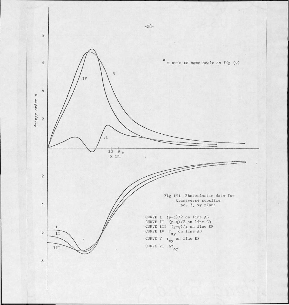
Figure (8) Photoelastic Data for TransverseSubslice No. 3, xy Plane _ _ _ _ _ _ _ _ _ _ _ _ 28
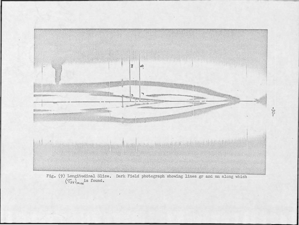
Figure (9) Longitudinal Slice _ _ _ _ _ _ _ _ _ _ _ _ _ _ _ 30
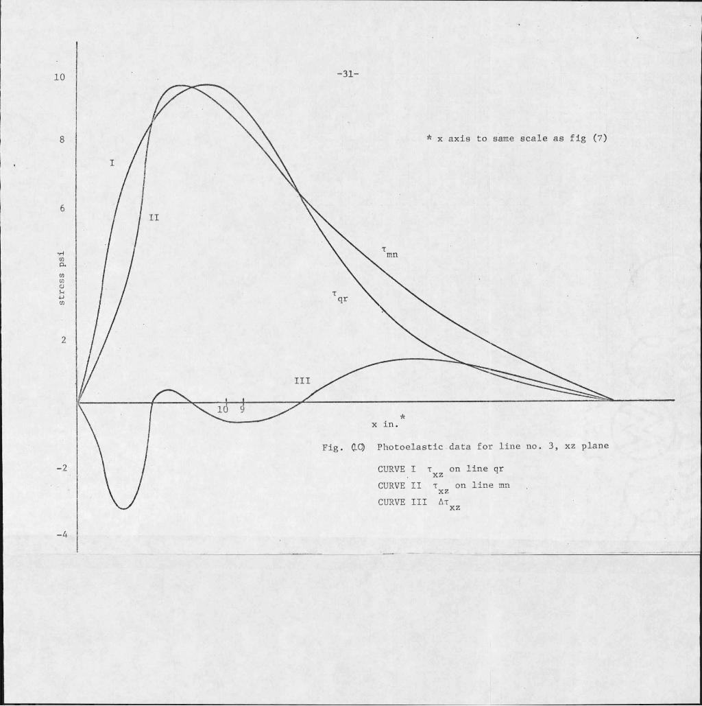
Figure (10) Photoelastic Data for Line Nb. 3,xy Plane _ _ _ _ _ _ _ _ _ _ _ _ _ _ _ _ _ _ _ _ 31
Figure (Il) • Comparison of Theoretical Two-Dimensional Contact Stress Distribution for the Sur- . face Configuration of the Central Plane of the Model and the Experimental Results on that Plane - _ _ _ _ _ _ _ _ _ _ _ _ _ _ _ _ _ 33
Figure (12) S^ice No.I _ _ _ _ _ _ _ _ _ _ _ _ _ _ _ _ _ _ 38
Figure (13). Slice No. 2 _ _'------------ ------------■-----39'
Figure (l4) Slice No..3 _ _ _ _ _ _ _ _ _ _ _ _ _ _ _ _ _ _ 40
Figure (15) Slice No. 4. 4l
Figure (16) Slice No. 5 42
Figure (I?) Dark and Light Field Photographs ofCalibration Disk _ _ _ _ _ _ _ _ _ _ _ _ _ _ 48.
Figure (l8) Fringe -Order n on a Horizontal Radius ofthe Calibration Disk _ _ _ _ _ _ _ _ _ _ _ _ _ _ _ 49
—vi—
List of Figures (continued)
' Page
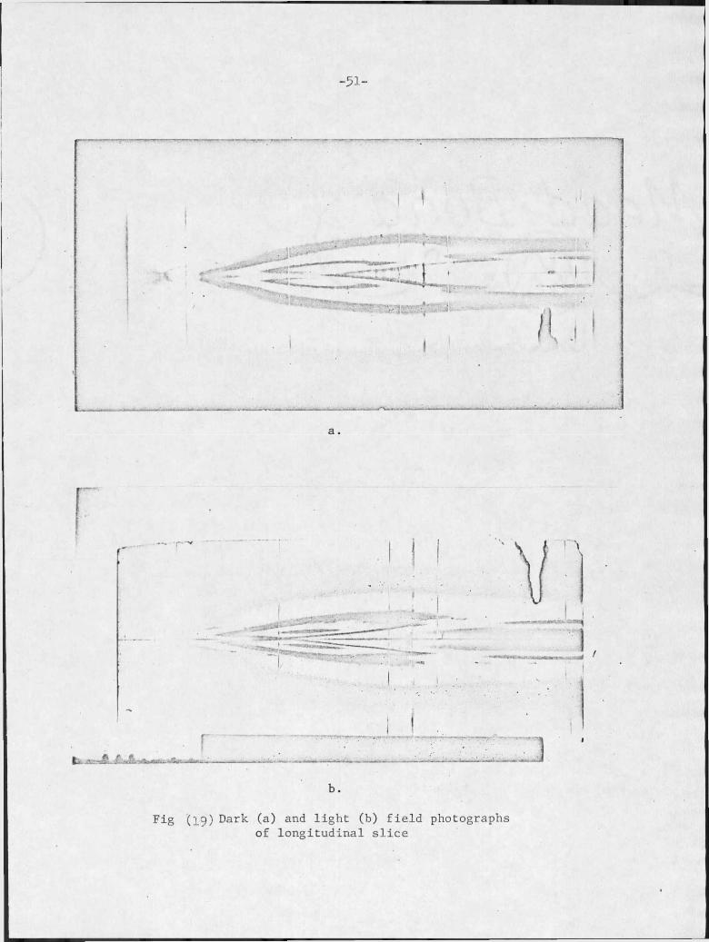
Figure (19) Dark and.Light Field Photographs ofLongitudinal Slice - - - - - - - - - - - - - - - 51
Figure (20) Light Field Photographs" of TransverseSubslices - - -- - - - - - - - - - - - - - - - - 52
Figure (21) Dark Field Photographs of Transverse Sub- -slices 53
Figure (22) Isoclinics in Transverse Subslices' - - - - - - - - 5k
-vii-
Abstract
The object of this investigation was to produce an accurate analysis of the contact stress distribution on a three-dimensional body. The case presented in this thesis was a photoelastic study of an elastic body with surface discontinuities, loaded between rigid planes.
A model, shaped similar to a roller bearing, was machined from an epoxy resin and loaded under a constant weight. The "frozen stress" method was then used in an analysis of the strains (stress) in the body and in the contact region in particular. Contact stresses were calculated using a Fortran program of the shear-difference equations and source data obtained from photographs of the photoelastic stress ^patterns in model slices.
The results of this investigation were compared with theoretical predictions of-contact stresses for a two-dimensional body of similar shape. The two-dimensional theory predicted higher contact stresses in the regions of discontinuities than were found actually to occur in the three-dimensional body.
CHAPTER I
INTRODUCTION AND PROBLEM STATEMENT
A rather special problem facing research and design people
today, particularly in the bearing industry, is the determination
of contact stresses between elastic bodies. Solutions have been
found by both theoretical and experimental means for three-dimensional-I
contact stresses (17,5)i but these solutions are currently restricted
to a small number of configurations. Unfortunately there is not a-
vailable a general analytical procedure for solving the contact stress
problem. The theory of elasticity ..does provide, a system of differ
ential equations that can be solved... for three-dimensional stresses,
but because of their complexity a solution is usually possible only
for very simple shapes.
In most cases an exact analytical solution to the contact stress
problem is unavailable, and so efforts to solve any particular contact
problem often turn to the methods of experimental stress analysis. ;
Since there is little chance of obtaining an accurate■solution to an
unsolved, configuration by extrapolating available experimental solu-'■
tions, each new contact problem will usually require a separate in-
vestigation. As might be expected, the number of experimentally-
solved problems is small, which makes the need for a relatively simple
and general analytical method of determining contact stresses obvious..
Numbers in parenthesis refer to the reference list at the end of the paper.
-Z-
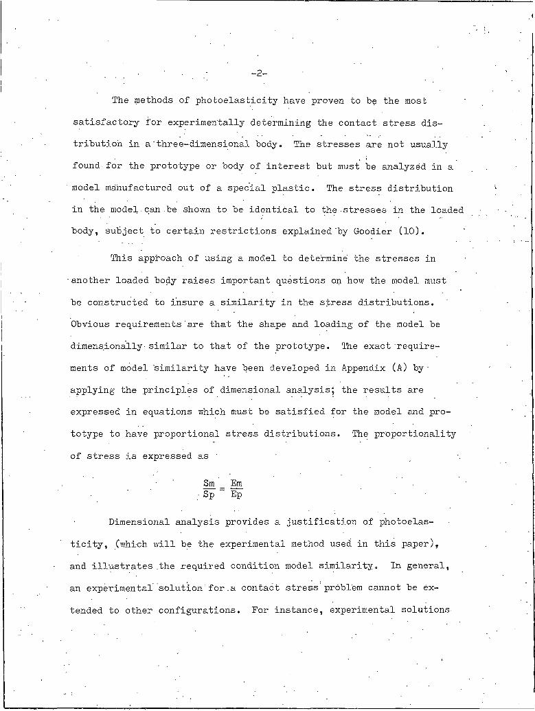
The methods of photoelasticity have proven to be the most
satisfactory for experimentally determining the contact stress dis
tribution in a ’three-dimensional body. The stresses are not usually -
found for the prototype or body of interest but must be analyzed in a model manufactured out of a special plastic. The stress distribution
in the model can be shown to be identical to the stresses in the loaded
body, subject to certain restrictions explained "by Goodier (10).
This approach of using a model to determine the stresses in
■ another loaded body raises important questions on how the model must
be constructed to insure a similarity in the stress distributions.
Obvious requirements are that the shape and loading of the model be
dimensionally- similar to that of the prototype. The exact require
ments of model similarity have been developed in Appendix (A) by -
applying the principles of dimensional analysis; the results are
expressed in equations which must be satisfied for the model and pro
totype to have proportional stress distributions. The proportionality
of stress is expressed as ' _
Sm _ Em ■ Sp Ep
Dimensional analysis provides a justification of photoelas
ticity, (which will be the experimental method used in this paper),
and illustrates the required condition model similarity. In general,
an experimental solution for.a contact stress problem cannot be ex
tended to other configurations. For instance, experimental solutions-
“3“
for contact stresses between spheres cannot be extended’ to find the
contact stresses between cylinders. Vdiat is desired,'then, is a
general analytical method of finding a solution to the contact stress
problem that is convenient and inexpensive.
An analytical technique for two-dimensional elasticity has been
developed by Blackketter (l) that frees an analysis of contact stresses
from the restraints imposed by the experimental method. Attempts are
being made to expand this two-dimensional theory and to develop other '
analytical tools .for accurately predicting three-dimensional contact
stress distributions.
For the accuracy of any analytical scheme to be evaluated some
reference is needed, some standard for comparison. Though the ex
perimental method of determining stresses by photoelasticity has many
shortcomings, it also has the outstanding strength of being quite,
accurate. Taking advantage of the accuracy of photoelasticity and
using the "frozen stress" technique, this paper will present an inves-1
tigation of contact stress on a three-dimensional body. .The results
will be used as a reference for an analytical solution using Black-
ketter’s method for the stress distribution on a plane of the three-
dimensional body.. It is hoped that the comparison might substantiate
Blackketter’s theory for three-dimensions or at least suggest new
approaches to an analytical solution.

CHAPTER II
THREE-DIMENSIONAL STRESS ANALYSIS BY PHOTOELASTICITY
2.1 An Outline of the Frozen Stress Method
In the nineteenth century, Maxwell, who was doing research
on torsion, heated an isinglass cylinder and applied a torsional load
to it. After permitting the cylinder to cool under load, he found
that the strains remained after the load was removed and if the cylin
der was placed in polarized light it exhibited a photoelastic effect.
This effect was apparently dismissed - until recently when M. Hetenyi
developed many of the techniques associated with the frozen stress
type of analysis."
The procedure of freezing stresses in' a body for photoelastic
purposes involves heating a plastic model to a certain temperature
(referred to as the critical temperature), loading the model at this
high temperature, and slowly cooling while maintaining the load. At.
room temperature the load is removed and the strains are found to be
permanently locked or annealed in the model. It is known that these
deformations represent an elastic distribution of stress if the yield
point of the plastic was not exceeded at the elevated temperature.
Slices removed from the model will not significantly distrub the ori
ginal elastic distribution of stress, and when viewed in a polariscope,
produce the same type of information as a two-dimensional photoelastic
analysis. The isochrornatic fringe patterns represent the difference
in maximum and minimum normal stresses in the plane of the slice; these
-5-
stresses are referred to as secondary principal stresses and are
usually different from the principal .stresses. The isochromatics
result from a relative retardation of light waves passing through.the
slice and so are an integral effect closely ,approximating the stresses
on the central plane'of the slice. The photoelastic fringe pattern
more accurately represents the shearing stress on a central plane of
a slice as the slice is made thinner. It is particularly desirable
to make the slices as thin as possible in regions of high stress
gradient.
2.2 Properties of Plastics'
The physical behavior of the .plastic used in three-dimension
al photoelasticity provides the basis for the experimental procedure.
The requirements for a material to be used in a "frozen stress" an
alysis are that the strains produced in the model under load at the
high temperature must remain in the plastic after cooling and all
strains must represent an elastic stress distribution. The plastic
should also be machinable into thin flat plates without disturbing the
original stress distribution, and the strains in the model should
duplicate strains in the prototype (model similarity).
The behavior of plastics that exhibit this property of
locking in the strains is explained by a diphase theory. It is assumed
that the plastic is structured of a completely polymerized internal
skeleton of molecules'and of.a surrounding amorphous'phase. The
strength of the molecular skeleton does not change much with tempera-
—6“
ture, but at the critical temperature the amorphous phase becomes
soft and carries only a minute portion of the total load. When the
■ plastic model in this investigation was heated to its critical tem
perature of 28.00F1 the modulus, of elasticity dropped from $00,000 psi
to 2000 psi. ' -
If the model is slowly cooled from the critical temperature
under stress, the soft viscous component will solidify around the
primary network holding or locking in the stress and displacements
the model underwent when loaded at the high temperature. -The cooled
model has a stress system in the primary network balanced by stresses
in the solidified viscous phase. Because these stresses are in equil- '
ibrium on a microscopic scale, sawing of the model will not appreci
ably disturb the displacements in the plastic„ Any planes removed from
such a model will exhibit the photoelastic effect, the only difference
from the two-dimensional problem being that the birefringence is pro
duced by the-secondary principal stresses (principal stresses in the
plane of the slice) instead of the principal stresses.
The properties of certain plastics that permit an elastic
stress distribution to be frozen into a loaded model and slices to be
cut from the model without disturbing the stress equilibrium make a
three-dimensional analysis possible. Photoelastic -data obtained from
certain slices in conjunction with the shear-difference equations (see
Chapter 4) make it possible to determine all six components of stress
at any point in the body. In the case to be considered in this inves
-7-
tigation, all that is required is one normal component the contact
stress. Because it is not possible to determine this stress directly
in the contact area, i.e., on the loaded surface, a somewhat indirect
method as explained in Chapter 4 will be used.
2.3 Requirements of a "Frozen Stress" Analysis
Although the details of a photoelastic analysis will vary
from problem to problem,' the general procedure usually involves the
construction of a model out of plastic, determining the optical pro
perties of the .plastic, loading and .freezing a deformation into the
plastic, slicing, recording the isoclinic and isochromatic fringe
patterns, and the reduction of the photoelastic data into meaningful
graphs. The "basic equipment required for -carrying out these steps in
a three-dimensional analysis includes a polariscope, an annealing oven
with programmed temperature control, loading frame, machine tools,
polishing wheels and photographic equipment and darkroom.

CHAPTER III
MODEL CONFIGURATION AND FABRICATION
3-1 Model Configuration
The model configuration of a nearly right circular cylinder
with end tapers that was used in this analysis is shown in Figure I.
The selection of a configuration took into account the limitations of
the two-dimensional analytical- solution that the results of this paper
were to be compared with, optical and material properties of the plas
tic, and the difficulty of accurately machining the- model.
Restraints on the two-dimensional theoretical development
required that the maximum deviation from contact of the surface of
the elastic body be of the order of the magnitude of the maximum
strain displacement in the body. Also, the surface-defining equations
must be continuous functions of position and their derivatives should
be small. These limitations require that the slopes of all points on
the surface be small but permit such complications as changes in cur
vature of the surface and transitions from a plane surface to a
curved one.
3«2 Selection of a Plastic .
Perhaps the most important performance feature of a photo
elastic material is its optical sensitivity; this property is expressed
as the amount of shearing stress required to produce a fringe. High
optical sensitivity in a plastic is shown by a low fringe contrast.
For instance, epoxy resin and plexiglass have material fringe con-
-9-
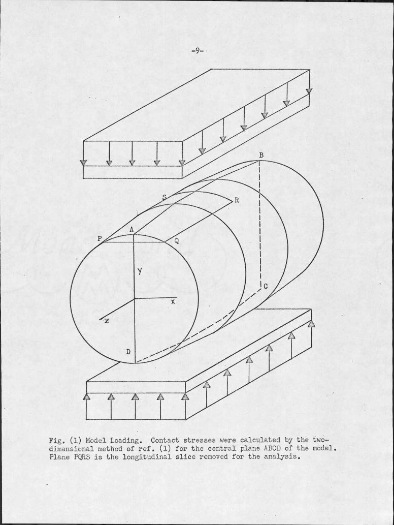
Fig. (I) Model Loading. Contact stresses were calculated by the two- dimensional method of ref. (I) for the central plane ABCD of the model. Plane PQRS is the longitudinal slice removed for the analysis.

—10—
slants, f, of 30 psi-in./fringe and 380 psi-in./fringe, respectively,
showing that the epoxy is almost 13 times as sensitive to stress as
plexiglass. The ratio of the material fringe constant to the modulus ■
of elasticity of the material' is a common way of evaluating the de
sirability of a three-dimensional photoelastic plastic. This ratio
gives a term commonly referred to as the figure of merit.
Q = E/f
Q = Figure of Merit
Other qualities of a plastic being equal, the highest figure of merit •
indicates the most desirable model material.
An epoxy, Hysol 4290, was finally settled upon and ordered
from the Hysol Corporation. The material, ordered in a cast cylinder
4 in. in diameter and 36 in. long, satisfied the above requirements
in addition to other important qualities of a photoelastic material
such as cost, availability, and a minimum of creep and time edge
effects. The' resin had a figure of merit of about 2000/.603 = 3320 at
the critical temperature, which made it more desirable from the- op
tical standpoint than any .other material considered.
3.3 Model Fabrication
The model shape used in this investigation is shown in
Figure 2. Ease in machining this model to close tolerances and a
straightforward formulation of the analytical computations were de
ciding factors in choosing this model configuration. The contact
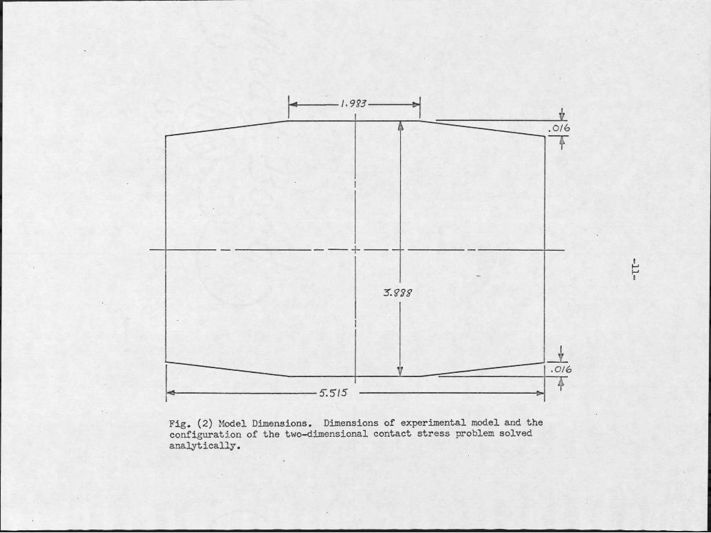
Fig. (2) Model Dimensions. Dimensions of experimental model and the configuration of the two-dimensional contact stress problem solved analytically.
-12-
problem was selected to be the tapered cylinder loaded between two
rigid planes; this condition was approximated by loading„the elastic
body in diametral compression between two steel plates.
To obtain the necessary photoelastic information, a model
had to be machined, loaded and annealed, and then sliced before the
analysis could be made. Using a high cutting speed and an open skip-
tooth blade on a bandsaw, a 7-in. length was first cut from the cast
cylinder, providing enough material for both a model and the necessary
calibration disk. After annealing to remove any residual stresses, the
piece was turned to a right circular cylinder. Tapers were then cut
on each end with the taper attachment, Reaving enough material in the
center section for it to be turned down to the design width. This
material is highly abrasive, quickly dulling and even burning tool steel
cutters. Since the surface finish deteriorated so quickly using tool
steel, it was found to be a good practice to use only a new carbide
tool reserved for work on these models. A cutting speed of 680 feet ■
per minute was -used along with a slow feed of .5 in. per minute to-
produce an excellent surface finish.
After machining, the actual.taper runout and other physical
dimensions were measured on an optical comparator that was accurate to
within j- 0.0001 in. Because the taper runout was so hard to set .ac
curately and machine on the lathe to the tolerance required, _+ 0.0005
in., it was sometimes necessary to machine the surface configuration
two or three times before symmetry was achieved.

-13-
3«4 Model Loading and Slicing
Loading the model- while it was being annealed meant that a
special loading frame had to be designed and built. A constant -weight
loading- arrangement was designed and built and appears in Figure (3).
Both the loading frame for the model and the calibration disk were -
fabricated from channel and angle iron. For the" model loading frame
the upper bar was constrained to move vertically by rollers on each
end, horizontal movement was controlled by a set screw through the
left vertical support. Ground steel plates were screwed to the channel for flat loading surfaces with pieces of plate glass placed be
tween the steel plates and the model in an attempt to reduce surface
friction.
The small calibration frame, seen to the left of the model
loading frame in Figure (3), was made specifically for disks to be
loaded in diametral compression. Scribe marks on the frame and disk
in conjunction with the parallel flat clamped to the rear of the frame
insured correct placement of the disk for symmetrical" loading.
The model was loaded by placing weights across the upper
channel and on the auxiliary, loading flat. These weights were posi
tioned prior, to starting the annealing or freezing cycle and held off
of the model by nuts on the threaded vertical supports. The model was
heated slowly to the critical temperature of 280°F at a rate of IO0F
per hour so .that induced thermal stresses would be kept to a minimum.
After the critical temperature had been reached and the model was in

r?*|"" .....- ..........
'-''t
=r-^;'.... :...
Fig, (3) Loading Frames and Annealing Oven
-15-
thermal equilibrium, the oven was opened and the nuts loosened so that
the upper channel rested on the model. Loading of the calibration
specimen at the same time was handled by removing a support that kept .
all weight off of the disk; in this way, both model and disk had'the
same temperature and loading history. Two hours elapsed at a con
stant temperature of 280°O before load was applied; then the model
was soaked for four hours before cooling below the critical tempera
ture. The model was cooled at a rate of 5 0F1Zhr. to room temperature.
This same cycle was used as an annealing cycle, to relieve residual
stresses from the cylinder before machining. . . . .
The final step after "locking in" the stresses prior to .
recording photoelastic data is the removal of certain planes from the
model. The selection of these planes is explained in the section on '
reduction of data. The model was sliced in a milling machine using a
3/l6-in. alternate-tooth side milling cutter, Figure (4-b). A four-
jaw chuck was used to hold the work for the longitudinal slice. The
slowest feed speed of the milling table of l/2-inch per minute was
used along with a cutter speed of 142 feet per minute. Higher cutter
speeds induced chatter and resulted in a poor surface finish.
3.5 Recording Isoclinics and Isochromatics
The photoelastic data consisted of photographs of the iso-
chromatic patterns and of sketches made on tracing paper of the iso-
clinic lines (Appendix (C) )„ To obtain this data the slicing plan shown
16-
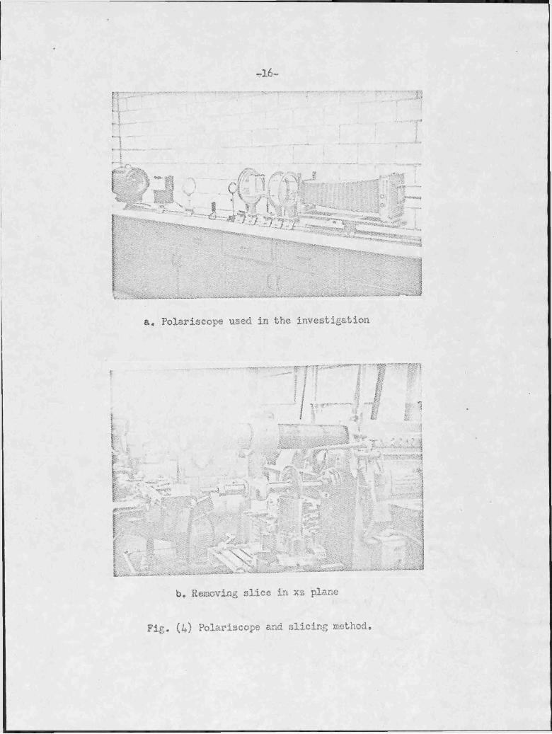
a, Polariscope used in the investigation
b, Removing slice in xz plane
Fig, (4) Polariscope and slicing method.
-17-
in Figure (5) was followed, each slice being analyzed in the polari-'
scope in exactly the same manner as if it were a two-dimensional
problem.
Isoclinics were recorded first to provide a reference in
using Tardy's method of compensation for determining fractional fringe
orders. Isoclinics were traced over the image thrown on the ground
glass camera screen in a plane polari'scbpe setup. Extreme care was
taken in finding isoclinic curves so that later computations for
shearing s'tress would have as small an error as possible. Isoclinic
curves often appeared in the image as broad black bands, making it
difficult to accurately find the actual center of the line. To aid
in tracing these lines the paper was taped to the top of the screen
so that it could be lifted and the image viewed directly. Points were
then picked that lay in the center of the curve and their positions
carefully noted on the screen; the point was then transferred to the.
tracing paper and its position rechecked= After several points were
located, particularly in the contact region, a smooth curve was drawn
and the final line again compared with the image.
Drawing the isoclinic lines for the top longitudinal slice
was difficult because of the vague -appearance of the curves. For an
idea of the general positions of these lines, the slice was watched
during several rapid rotations of polarizer and analyzer. This pro
cedure gave an idea of the isoclinic development; each isoclinic line
was then sketched on a separate sheet of paper and a final sketch was
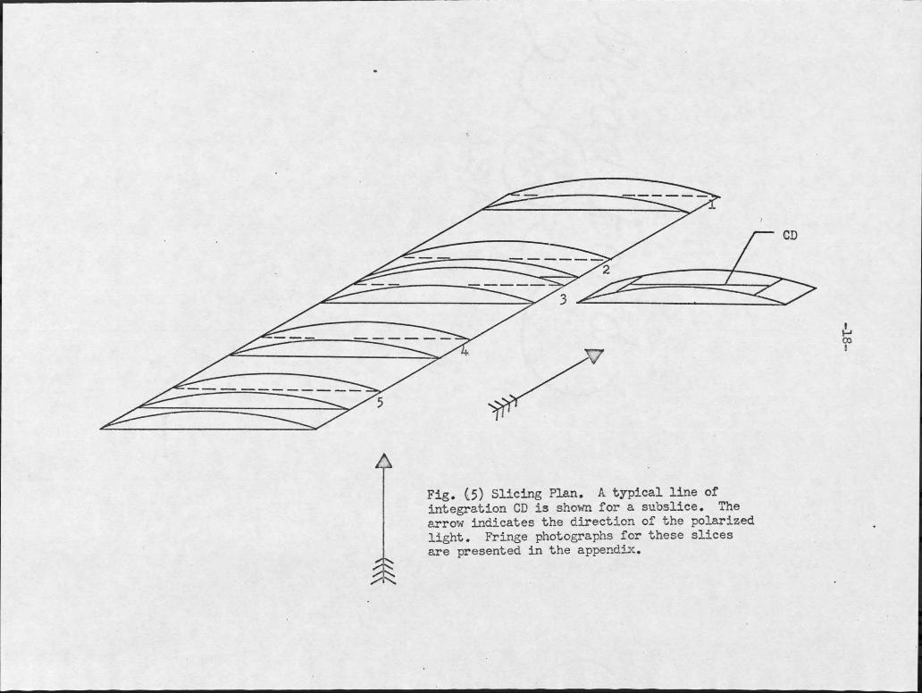
Fig. (5) Slicing Plan. A typical line of integration GD is shown for a subslice. The arrow indicates the direction of the polarized light. Fringe photographs for these slices are presented in the appendix.
-19-
made of all lines on one sheet. This last sketch was a valuable guide
in sketching isoclinics under high magnification.
A considerable reduction in time and effort was' effected by
making the isoclinic diagrams quite large for the regions of interest
and then making isochrornatic prints to the same scale. The lines of
integration were.then drawn on the photographic prints as in Figure
( 6) i and the isoclinic tracing fastened over the print.
Isochromatics were evaluated using a monochromatic light
source, circular polariscope, and photographing the resulting fringe
pattern. Tardy's method of compensation was used to determine fraction
al fringe orders to with _+ 1/25' fringe (ll). This method depends upon
the fact that if the axis of the polarizer and analyzer are aligned
parallel to the directions of the principal stresses in the model slice
a rotation of the analyzer will give a proportional shifting of the
fringes to a higher or lower order. If the polariscope is aligned to
find the fringe order at a point and a rotation of the analyzer from
a dark field setup moves the fringe through the point towards a higher
order fringe, the fringe order is found from the relation
n = lower order fringe + .. —
If the fringe moves from, the higher order to the lower order fringe
the following relationship is used.
n = higher order fringe- .an£ ^ ..

-20-
The fringe order for a rotation of $0° of the analyzer
n = fringe order — ^ = fringe order _+ 1/2 -180
is just the relative retardation observed in a light field polariscope.
A limitation of the above method of compensation is that only frac
tional orders of fringes can be found. The absolute magnitude must
be found from a knowledge "of the- fringe pattern", examination in a ■
plane polariscope, or compensation by some other method.
5.6 Equipment
A great deal of effort was spent trying to get a parallel,
uniform field of light and high fringe resolution. .The original polar
iscope left much to be desired in these respects and many different
setups were tried before a final arrangement was settled upon.. The
final polariscope setup is shown in Figure (4-a). For a uniform field
of light a diffuser made of sanded Incite was placed over the hole used
to approximate a point source of light. The effects of parallel light
needed for a sharp boundary and good fringe definition was approximated
by making the distance between the condensor lens and model slice as
long as possible and by stopping down the aperture of the camera lens.
These techniques made possible a clear resolution of fringes in the
region of high stress gradient (Il).
Light and dark field isochromatic fringe patterns were re
corded on photographs, two for each transverse slice and two for the
longitudinal slices. Kodak contrast process panchromatic film was
- 21-
developed in HC-IlO developer for maximum contrast negatives. Prints
were made on Kodak medalist P-4 photographic paper. Exposure time
ran up to 30 seconds with a shutter opening of f-32.
CHAPTER IV
COMPUTATION OF CONTACT STRESSES
4.1 Shear-Difference Equations
A complete solution of the three-dimensional stress problem
requires the determination of the six independent cartesian stress
components from six equations; however, this investigation is con
cerned with finding only contact stresses. The orientation of the co
ordinate system, Figure (l), makes the problem one of finding cr̂ along
the contact surface. Of the methods available, the shear-difference
method, which has been used extensively in two-dimensional elasticity
(7), was chosen as' being the most direct and least troublesome for
the determination of the contact stress distribution.■
The shear-difference method utilizes the equations of equi
librium from the theory of .elasticity. Neglecting body forces, the
equilibrium equations for a three-dimensional body are
I. _.yx + _.. -z*^ y «2 Z
dT2.
9 y■xy<9 x
■2 %
5 r̂ Z XZ , 97V z^ X ^ y
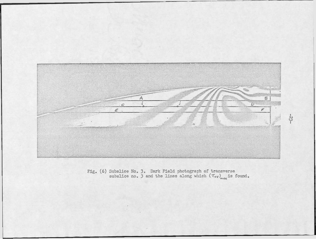
Fig. (6) Subslice No. 3. Dark Field photograph of transversesubslice no. 3 and the lines along which (Txv) ^ i s found.

—24—
Assume that the distribution of stress is known and let
points i and j be general points in the body, Figure (5). To deter
mine one normal component of stress at a point, only one of the equi
librium equations need be solved because the orientation of a co
ordinate system is arbitrary.
Thus, equation 3 can be written in the form
J a crX 1— -— dx = - — — dxJ i 9 x i J-resulting- in
dr XZ dx
4. (o' ). = (Cf ).• x J X lj 2Txyii ai
dx0i d Z
Equation 4 is referred to as the shear-difference equation and by
rewriting it in finite difference form it will be of most use in
this analysis.
d A^yvx d A r zx5- «V3 - cIi - f Ax - ITo determine at a point j, three terms must be known (c^v)x i5
-25-
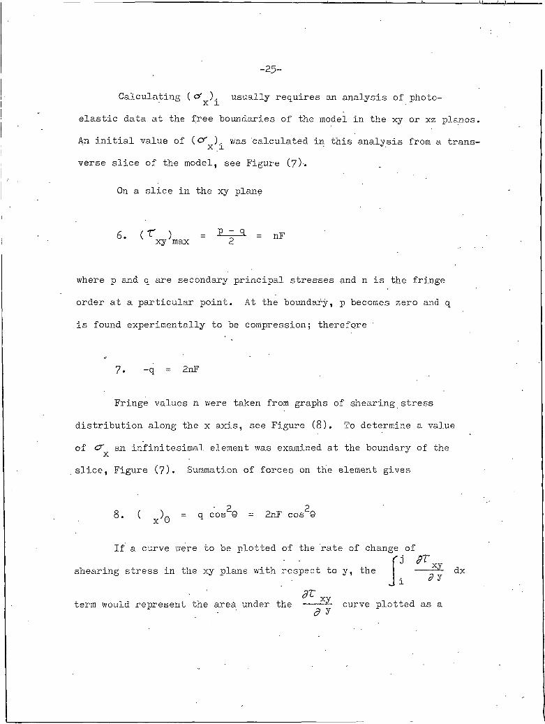
Calculating ( usually requires an analysis of photo
elastic data at the free boundaries of the model in the xy or xz planes
An initial value of (o' ) was calculated in this analysis from a trans'
verse slice of the model, see Figure (?)-.
On a slice in the xy plane
6 . ( T xy max nF
where p and q are secondary principal stresses and n is the fringe
order at a particular point. At the boundary, p becomes zero and q
is found experimentally to be compression; therefore '
7. -q = 2nF
Fringe values n were taken from graphs of shearing stress
distribution along the x axis, see Figure (8). To determine a value
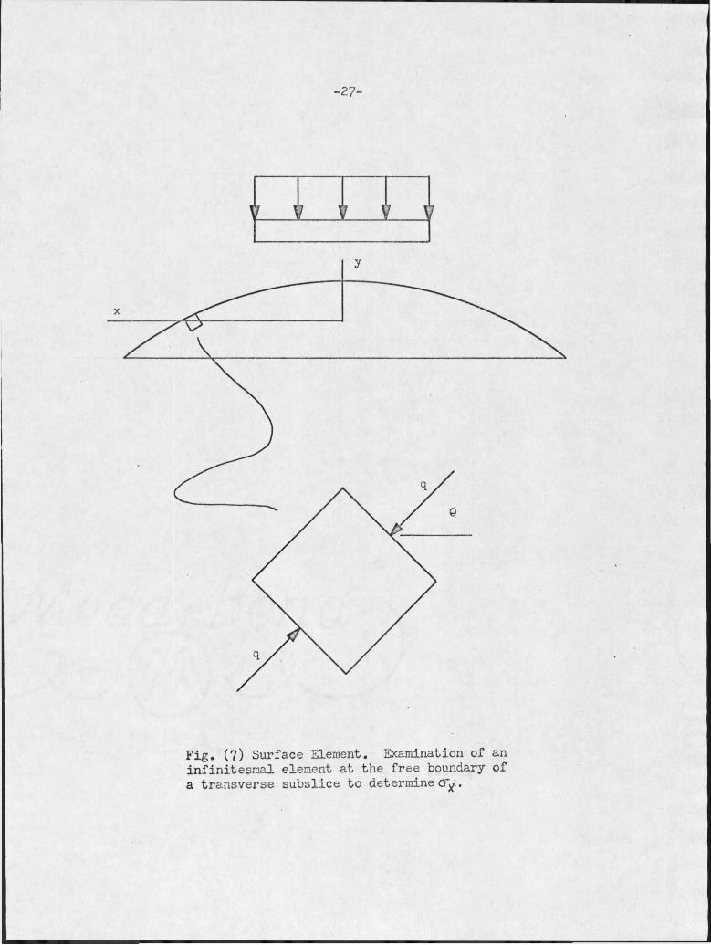
of o' an infinitesimal element was examined at the boundary of the
slice, Figure (?)• Summation of forces on the element gives •
8. ( %.)Q• 2 2 q cos 9 = 2nF cos 0
If a curve were to be plotted of the rate of change of
shearing stress in the xy plane with respect to y, the 22Li Z y dx
term would represent the area under thedT
d ycurve plotted as a
-26-
function of x. In finite-difference form the integral
j, ar
j'SLy
may be expressed as ^ . J£La y A 2c. To best approximate the area
under a curve of c?T— - a mean value of A T is used, a value<9 y xy
located halfway between points i and j.
Graphs of shearing stress along auxiliary lines AB and EF
(Figure (6) were drawn, Figure (8), from photoelastic data and the
A T distribution was plotted as a difference, in these curves. A
value of A T ^ was taken from the graph of AT^. halfway between
neighboring points i and j. The A x and Ay terms are the distances
between i and j and the auxiliary lines, respectively'. Similar com-A T
putations in the xz plane yielded a value for the xza y Ax
term in equation 7* Complete information for determining .a T and
A T xz is given by the curves of Figure (8).
Care should be taken in using a sign convention for A T ,
Ax,. ̂ Ay, and A z. For the right-handed coordinate system used, Ax,
A y ? and A z will have a positive value when integrating from i to j.
The sign of A T and A T depends on the magnitudes of shearing xy xzstress on the auxiliary lines.
Computation of O' was done with the aid of the computer program A ' ^in Appendix (D). The normal stress component at a general point j
can be calculated from values of O' and photoelastic information in
-27-
Fig. (7) Surface Element. Examination of an infinitegmal element at the free boundary of a transverse subslice to determine CTy.
fringe o
rder
8

-29-
'the xy plane from the equation
(C x O' ) .y j
9.py TrI-
(p - q) . cos 0 .J- J
( ) . - 2n;.F cos^x J 0 0 .J
Values of had to be computed below the surface because
the fringes photographed in the model slices represented an average
stress assumed to exist at the center of. each slice. If the longi
tudinal slices are approximately .0.1 in. thick, the shearing stresses
computed from the fringes in Figure (9) will represent values of ^ xz
on a plane of .05 in. below the contact surface and values calculated
for o' in equation 5 can be no closer than this to the contact
surface.
4.2 Sample Computation
As" an example of the computation of at a point on the
line of integration, consider slice #3 in Figure (5). Assume that
has been found for a point on the line CD, that will be designated as
station 9i and is to be calculated for station 10. Complete photo
elastic information is given in Figure (8) and Figure (10). Using
shear-difference equation no. 5
A x A y A T A x
A z
is found.V XV /m a x
stress p
si-31-
* x axis to same scale as fig (7)
x in.
on line qrCURVE I Ton line mnCURVE II T
CURVE III At
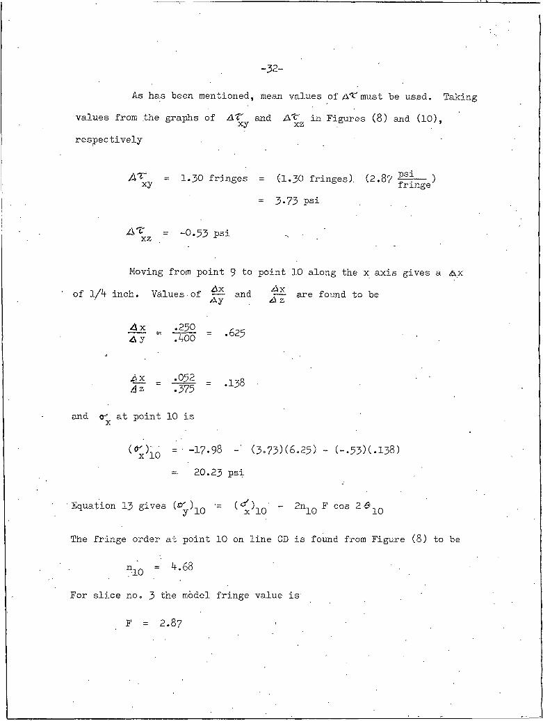
-32-
As has been mentioned, mean values of must be used. Taking
values from .the graphs of AT^. and in Figures (8) and (10),
respectively
= 1.30 fringes = (I.30 fringes). (2.8? — )xy fringe= 3-73 psi
= -O.53 psi .
Moving from point 9 to point 10 along the x axis gives a Ax
of 1/4 inch. Values of and I— are found to beAy A z
A x .250A y .400
_ .032d 2 .375
point 10 is
.625
.138 -
(r.)lQ = -17.98 - (3.73)(6.25) - (-.53)(.138)
=• 20.23 psi
Equation 13 gives (C^)iq - “ 2n10 F cos 2 ^ 10
The fringe order at point 10 on line CD is found from Figure (8) to be
n.j_Q = 4.68
For slice no. 3 the model fringe value is'
F = 2.87
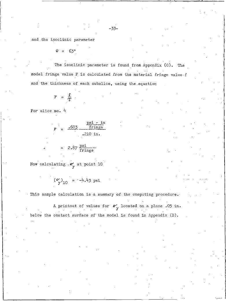
-33-
and the isoclinic parameter
63'
The isoclinic parameter is found from Appendix (C). The
model fringe value F is calculated from the material fringe value•f
and the thickness of each subslice, using the .equation
_fT
For slice no. 4
.603psi - in fringe
.210 in.
2.8? psifringe
Now calculating at point 10
cV i o = " - M 3 psi
This sample calculation is-a summary of the computing procedure.
A printout of values for located on a plane .05 in,
below the contact surface of the model is found in Appendix (D).
CHAPTER ¥
EXPERIMENTAL AND ANALYTICAL RESULTS
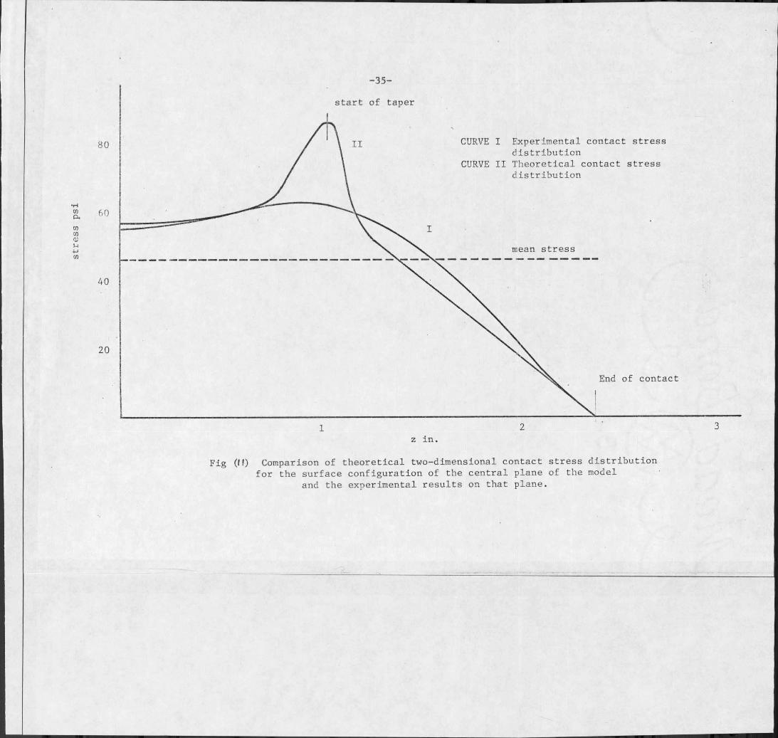
5.1 A Comparison of Experimental Results with a Two-Dimensional
Analytical Solution
A.solution for the contact stress distribution on the cen
tral yz plane of the model, using a two-dimensional analytical method,-
ref. (I), is compared with the three-dimensional experimental results
of this investigation in Figure (Il). In the graph of experimental
contact stresses the values plotted for the surface were taken from
the experimental results on a plane 0.05 in. below the contact sur
face. It is seen that the theoretical solution contact length was com-■
puted to be the same length as that found experimentally. The area
under the two-dimensional curve was made- equal to the area under the
experimental curve, so that the actual loading of-the model and the
assumed loading in the theoretical case were equal. By dividing these
areas by the common contact length a mean stress can be found. Com
paring the maximum theoretical stress to the mean stress and the maxi
mum experimental stress to the mean stress gives
I. Theoretical comparison
2. Experimental comparison
maxCfmean
86.2 in£
45.5 in"
1.99
maxmean,
1.46
lb65.0 in"
lb43.3 in"
stress p
si-35-
start of taper
CURVE I Experimental contact stress distribution
CURVE II Theoretical contact stress distribution
mean stress
End of contact
z in.
Fig (H) Comparison of theoretical two-dimensional contact stress distribution for the surface configuration of the central plane of the model
and the experimental results on that plane.
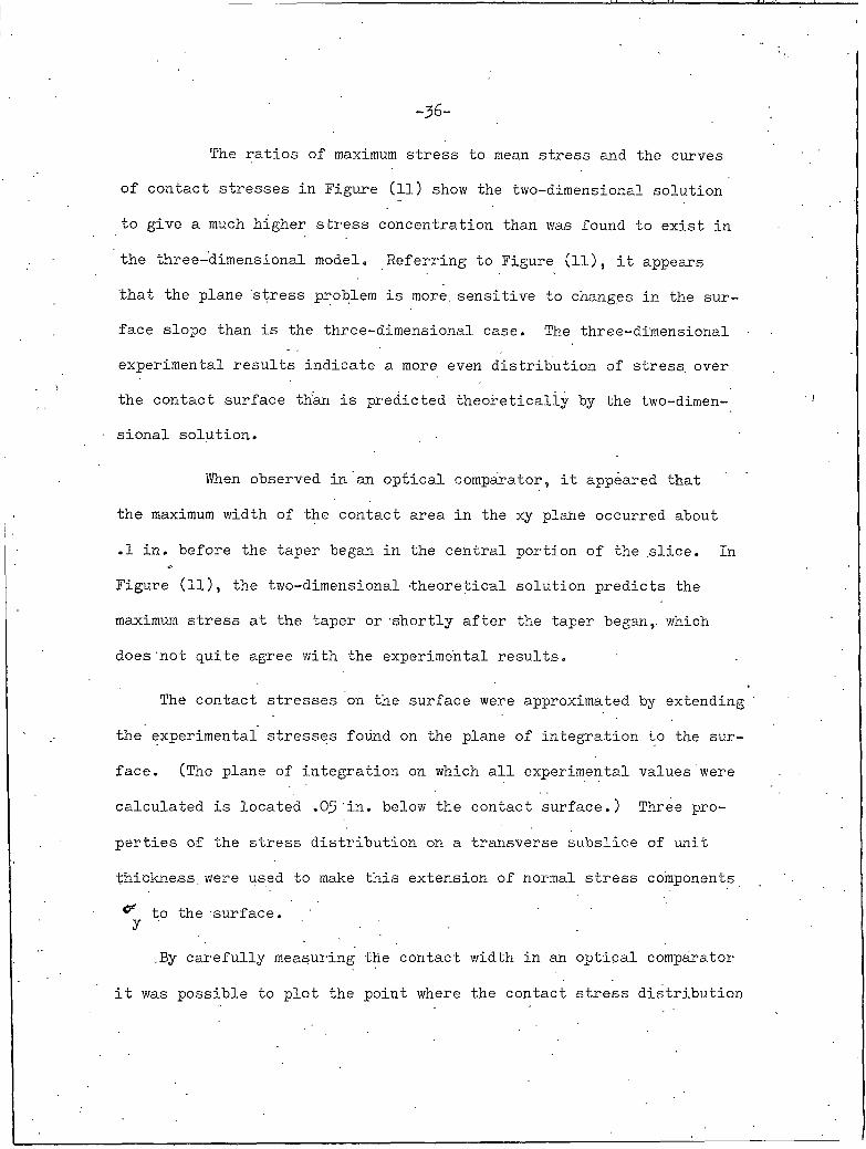
-36-
The ratios of maximum stress to mean stress and the curves
of contact stresses in Figure (Il) show the two-dimensional solution
to give a much higher stress concentration than was found to exist in
the three-dimensional model. Referring to Figure (11), it appears
that the plane stress problem is more, sensitive to changes in the sur
face slope than is the three-dimensional case. The three-dimensional
experimental results indicate a more even distribution of stress, over
the contact surface than is predicted theoretically by the two-dimen
sional solution.
VAien observed in an optical comparator, it appeared that
the maximum width of the contact area in the xy plane occurred about
.1 in. before the taper began in the central portion of the .slice. In
Figure (11), the two-dimensional theoretical solution predicts the
maximum stress at the taper or shortly after the taper began,, which
does not quite agree with the experimental results.
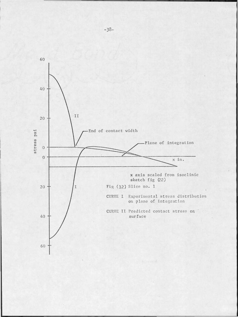
The contact stresses on the surface were approximated by extending
the experimental stresses found on the plane of integration to the sur
face. (The plane of integration on which all experimental values were
calculated is located .05 'in. below the contact surface.) Three pro
perties of the stress distribution on a transverse subslice of unit
thickness.were used to make this extension of normal stress components
^ to the surface.yBy carefully measuring the contact width in an optical comparator
it was possible to plot the point where the contact stress distribution
-37-
goes to zero. In this investigation'the relative magnitudes of the
contact stresses in the central portion of the contact width assured
a fairly accurate curve definition. It was assumed that the contact
stress distribution had essentially the same shape as- the normal
stresses on the plane of integration in the region where the values
of were large. , .
The third consideration was a requirement, that the stresses
on the plane of integration be in equilibrium with stresses on the con
tact surface.• Integration of the subsurface stress curve yielded a
value required for the area of the contact .stress curve.
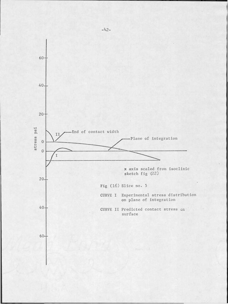
The contact stress distribution in the xz plane was obtained by using the shape of the curve on the plane of integration in regions
of high normal stress, requiring that this curve go through the point
where contact ends, and scaling the curve so that its area as measured
with a plainimeter was equal to the net area of the normal stresses
on the plane of integration. This resulted in the contact stress dis
tributions pictured in Figures (12-16). It is thought that these
distributions closely approximate the true contact stresses.
A static equilibrium check was made on the experimental re
sults by computing the approximate total volume under the predicted
contact stress distribution and comparing it to.the known loading.
stress p
si-38-
60
End of contact width
Plane of integration
x in.
x axis scaled from isoclinic sketch fig (22)Slice no. I
Experimental stress distribution on plane of integration
CURVE
CURVE II Predicted contact stress on surface
stress p
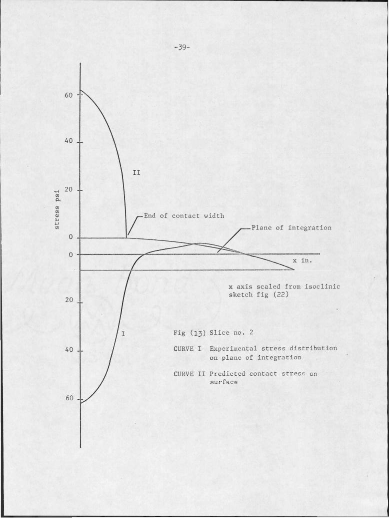
si-39-
x axis scaled from isoclinic sketch fig (22)
Fig (13) Slice no. 2
CURVE I Experimental stress distribution on plane of integration
CURVE II Predicted contact stress onsurface
40
60 __
stress p
si-40-
60 - -
40 --
20 - -
20 - -
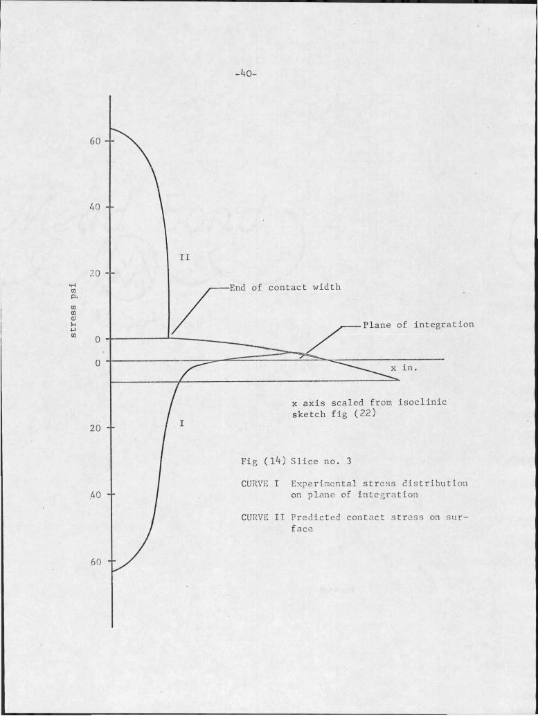
•End of contact width
Plane of integration
x axis scaled from isoclinic sketch fig (22)
Fig (14) Slice no. 3
40CURVE I Experimental stress distribution
on plane of integration
CURVE II Predicted contact stress on surface
60
stress p
si-4l-
40 --
20 - -
00
20 - -
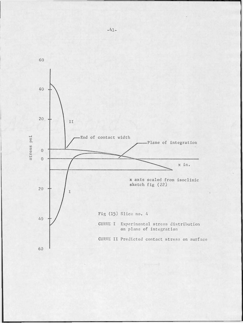
Plane of integration
x in.
x axis scaled from isoclinic sketch fig (22)
Fig (15.) Slice no. 4
CURVE I Experimental stress distribution on plane of integration
CURVE II Predicted contact stress on surface
60
stress p
si-42-
60--
40--
20- -
40--
Fig (16) Slice no. 5
CURVE I Experimental stress distribution on plane of integration
CURVE II Predicted contact stress on surface
60--
-43-
4.2 Conclusions
The three-dimensional experimental results of this paper
cannot be predicted accurately by the two-dimensional theory of ref
erence !(I). In general, the contact stress, distribution in three-
dimensional problems■differs significantly from two-dimensional solu
tions. However clever and ingeneous the assumptions, it does not
seem possible to accurately predict the contact stresses on a three-
dimensional body using two-dimensional solutions.
It is believed that the results of this paper provide an
accurate reference for comparison with analytical methods for predic
ting. contact stresses on three-dimensional bodies.
APPENDIX A
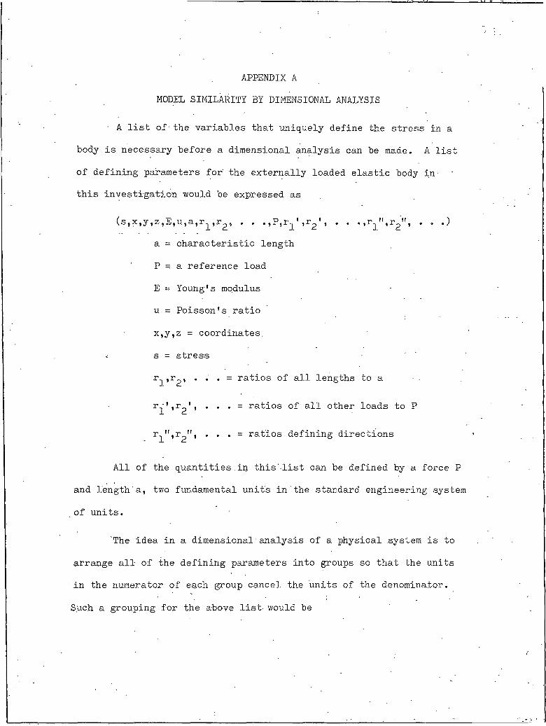
MODEL SIMILARITY BY DIMENSIONAL ANALYSIS
■ A list of-the variables that uniquely define the stress in a
body is necessary before a dimensional analysis can be made. A list
of defining parameters for the externally loaded elastic body in-
this investigation would be expressed as
(s,x,y,z,E1Uja1T11T2, . . .,P,^',^', . . 'Ir1lV 2",
a = characteristic length
P = a reference load
E = Young's modulus
u = Poisson's ratio
Xjy1Z = coordinates,
s = stress
rI5r2’ " " * = ra^ios of all lengths to a
T1',Tg', . . . = ratios of all other loads to P
^",r ", . . . = ratios defining directions
.)
All of the quantities ,in this'.list can be defined by a force P
and length a, two fundamental units in the standard engineering system
of units.
The idea in a dimensional analysis of a physical system is to
arrange all of the defining parameters into groups so that the units
in the numerator of each group cancel the units of the denominator.
Such a grouping for the above list, would be
-45-
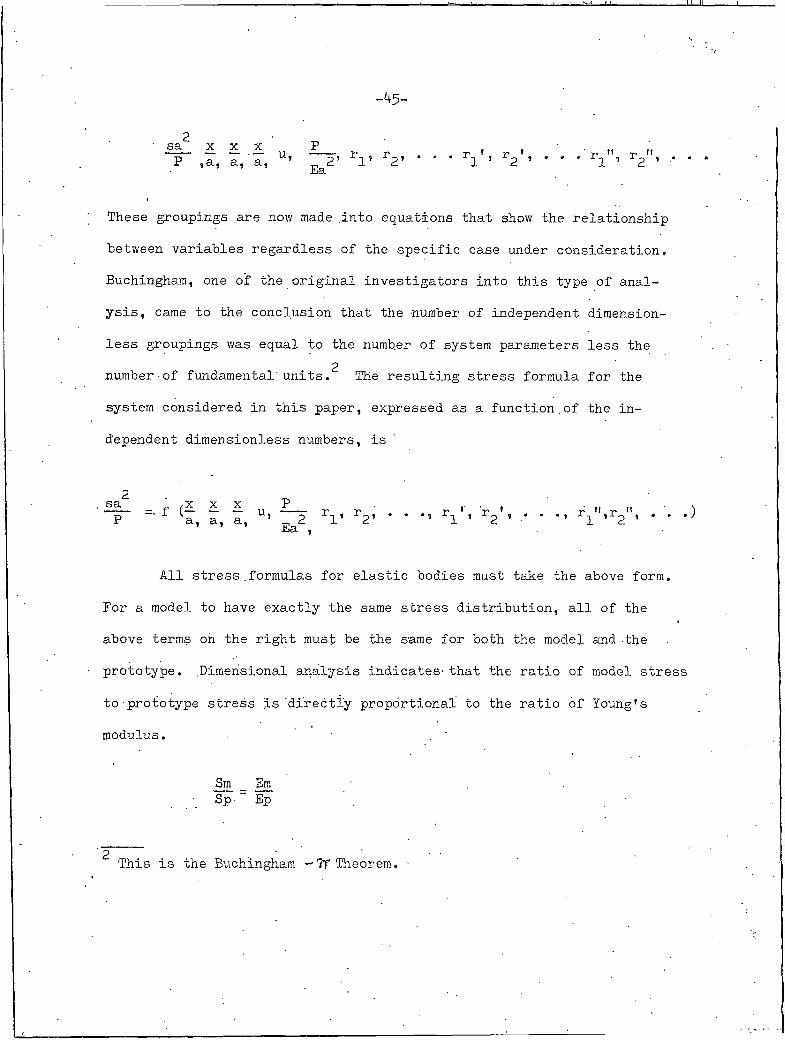
2 Psa x_ x.P ,a, a, a, Ea2 ’ rI’ r2’
These groupings are now made .into equations that show the relationship
between variables regardless of the specific case under consideration.
Buchingham, one of the original investigators into this type of anal
ysis, came to the conclusion that the number of independent dimension
less groupings was equal to the number of system parameters less the2number•of fundamental' units. The resulting stress formula for the
system considered in this paper, expressed as a function.of the in
dependent dimensionless numbers, is
All stress.formulas for elastic bodies must take the above form.
For a model to have exactly the same stress distribution, all of the
above terms oh the right must be the same for both the model and - the
prototype. .Dimensional analysis indicates- that the ratio of model stress
to prototype stress is 'directly proportional to the ratio of Young’s
modulus.
Sm Em Sp-~ Ep
2 This is the Buchingham -Tf Theorem. -
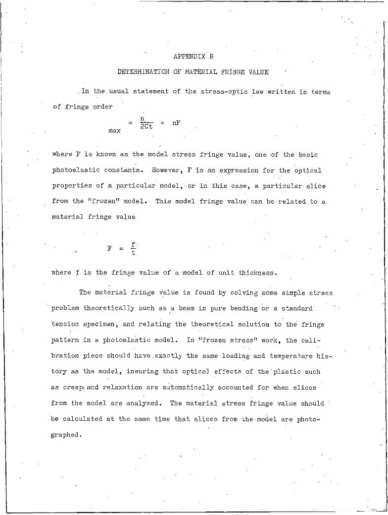
APPENDIX B
DETERMINATION OF MATERIAL FRINGE VALUE
. In the usual statement of the stress-optic law written in terms
of fringe order
maxn2Ct " nF
where F is known as the model stress fringe value, one of the basic
photoelastic constants. However, F is an expression for the optical
properties of a particular model, or in this case, a particular slice
from the "frozen" model. This model fringe value can be■related to a
material fringe value
where f is the fringe value of a model of unit thickness,
The material fringe value is found by solving some simple stress
problem theoretically such as a beam in pure bending or a standard
tension specimen, and relating the theoretical solution to the fringe
pattern in a photoelastic model. In "frozen stress" work, the cali
bration piece should have .exactly the same loading and temperature his
tory as the model, insuring that optical effects of the'plastic such
as creep)and relaxation are automatically accounted for when slices
from the model are analyzed. The material stress fringe value should
be calculated at the same time that slices from the model are photo
graphed.
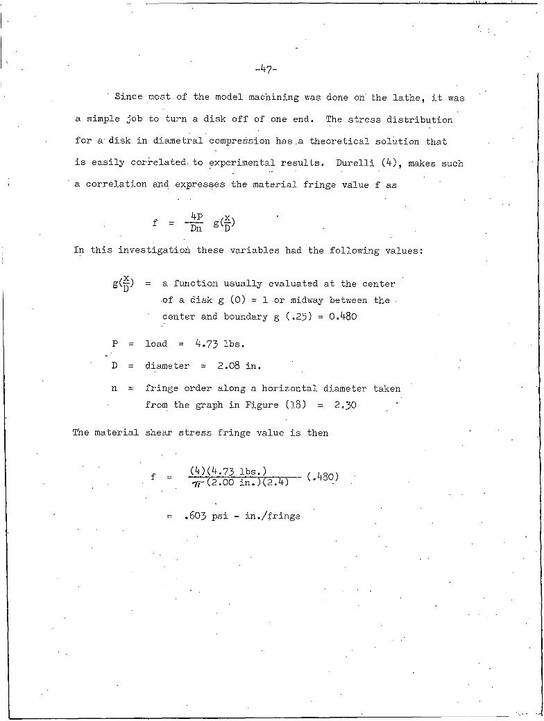
-47-
Since most of the model machining was done on the lathe, it was
a simple job to turn a disk off of one end. The stress distribution
for a disk in diametral compression has .a theoretical solution that
is easily correlated-to experimental results. Durelli (4), makes such
a correlation and expresses the material fringe value f as
In this investigation these variables had the following values:
g(^) = a function usually evaluated at the center■of a disk g (0) = I -or midway between the ■ center and boundary g (.25) = 0.480
P = load = 4.73 lbs.
D = diameter = 2.08 in.
n = fringe order along a horizontal diameter taken from the graph in Figure (l8) = 2.30
The material shear stress fringe value is then
f (4X4.73 lbs.)TT (2.00 in. )(2.4) (.480)
.603 psi - in./fringe
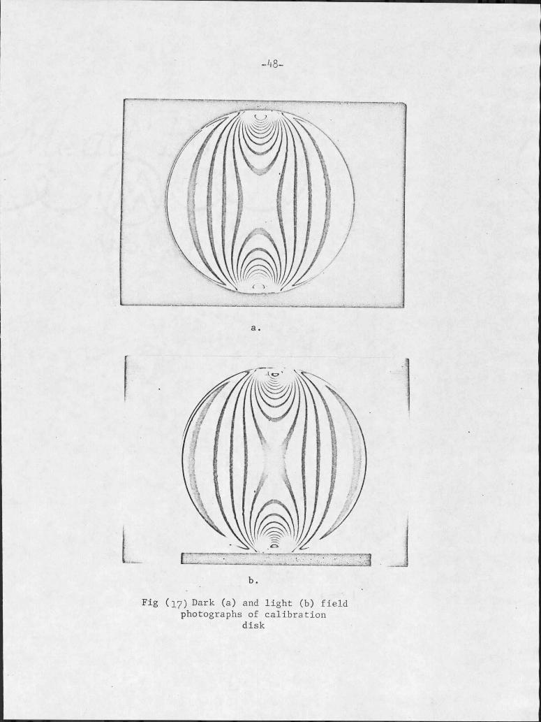
-48-
a.
Fig (17) Dark (a) and light (b) field photographs of calibration
disk
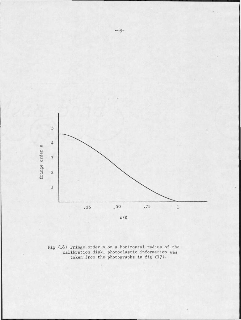
x/R
Fig (18) Fringe order n on a horizontal radius of the calibration disk, photoelastic information was
taken from the photographs in fig (I?)•

APPENDIX C
PHOTOELASTIC DATA
r , ~ . .4
-51
T~ rX
. 'I — 1I
rb .
Fig (19) Dark (a) and light (b) field photographsof longitudinal slice
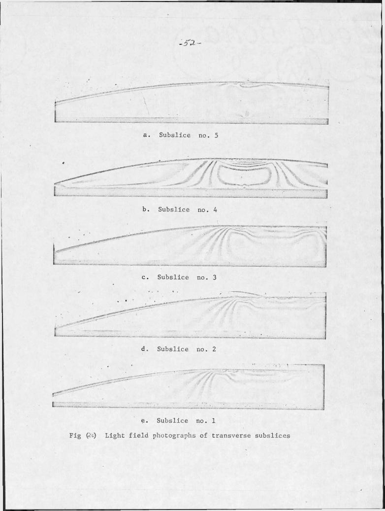
a. Subslice no. 5
Subslice no. 4
Subslice no. 3
Fig (?t) Light field photographs of transverse subslices
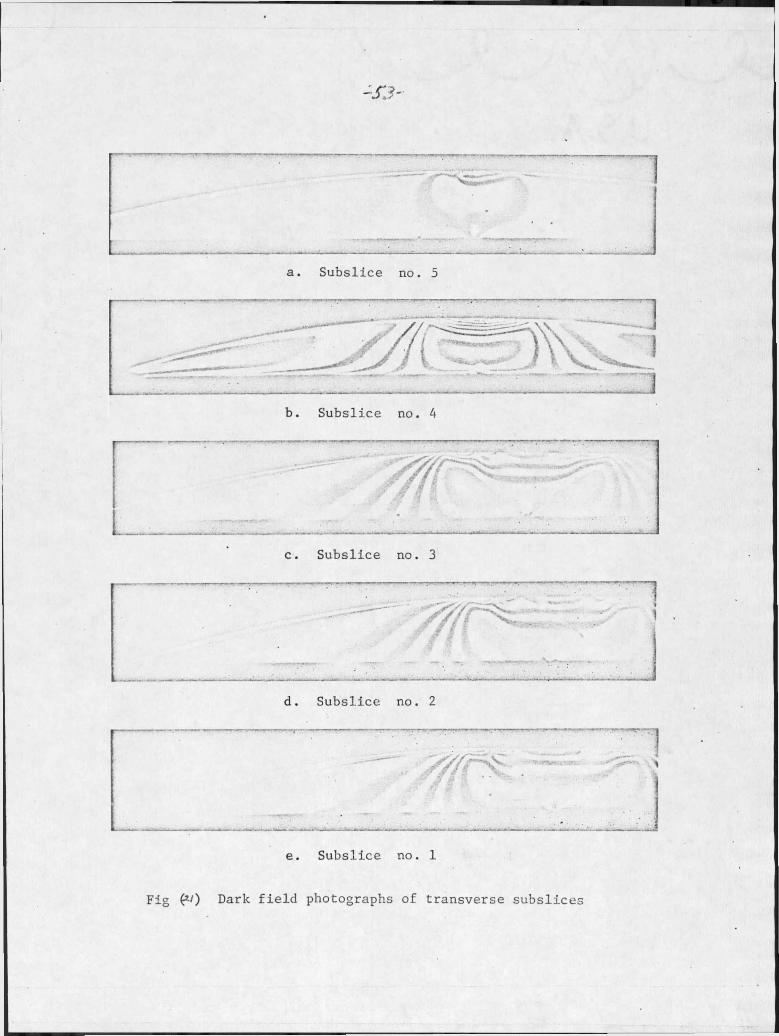
c. Subslice no. 3
e. Subslice no. I
Fig (*/) Dark field photographs of transverse subslices
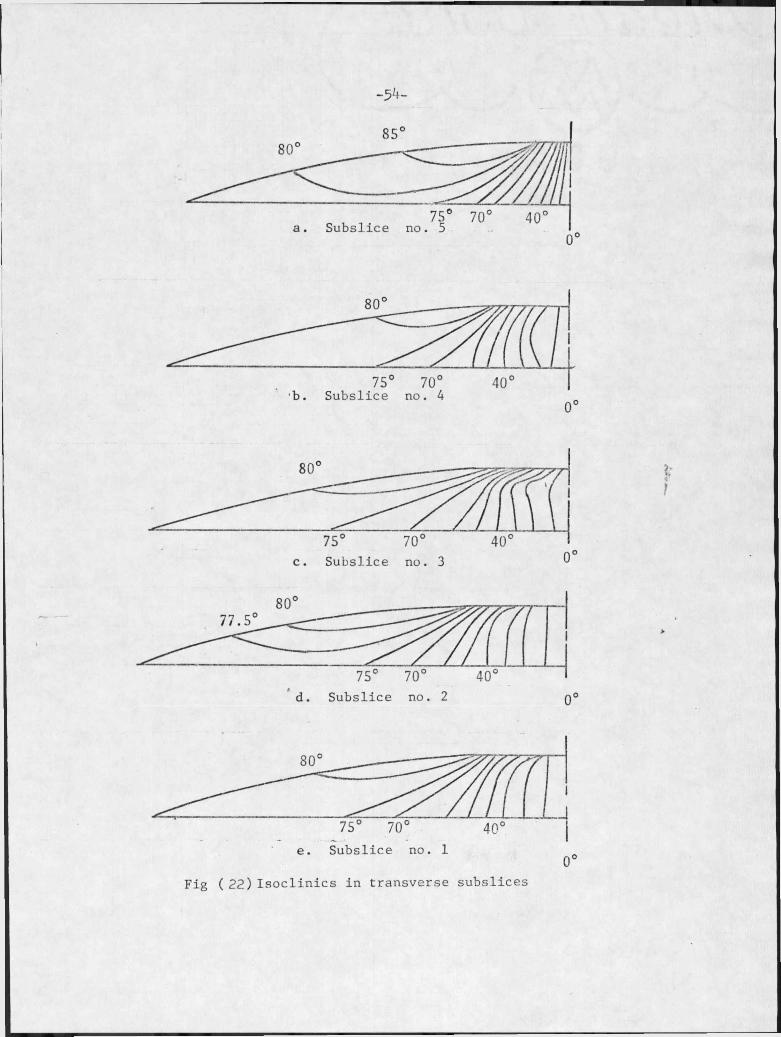
-54-
Subslice no. 5
Subslice no. 4
Subslice no. 3
Subslice no. 2
Subslice no. I
Fig ( 22)Isoclinics in transverse subslices
APPENDIX D
COMPUTER PROGRAM FOR CALCULATING (f AND RESULTSI
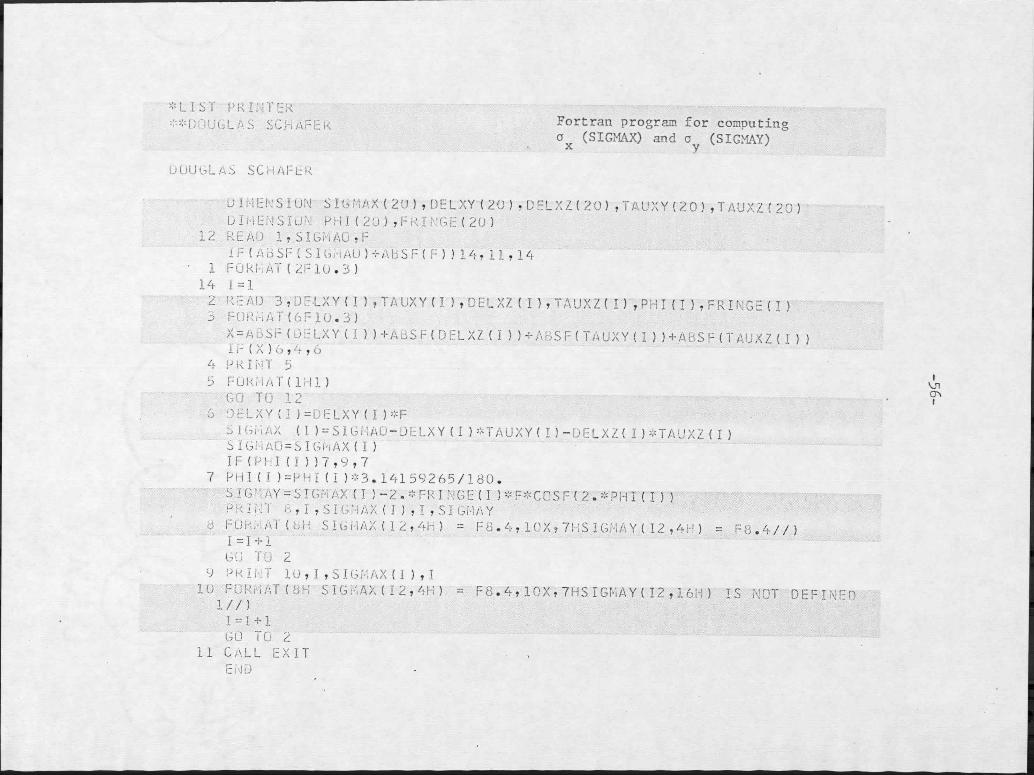
*LIST PRINTER **UnUGLAS SChAFEK Fortran program for computing
Ox (SIGMAX) and o (SIGMAY)
DOUGLAS SCHAFfcR
DIMENSION SIGMAX(ZU),UELXY(ZU).DELXZ(ZU),TAUXY(20),TAUXZ(20) DIMENSION RHI(ZU),FRINGE (ZU)
12 READ I,SIGHAOfFIF ( AoSF ( S IGi-IAU ) -:-AbSF ( F)) 14. 11,14
■ I FORMAT(ZF10.3)14 I = I2 READ 3,UFLXY(I),TAUXY(I),DELXZ(I),TAUXZ(I),PHI(I),FRTNG=fI)3 FORMAT(6F1U.3)X=ADSr(uFLXYd))+AbSF(DELXZ(I))+AKSF(TAUXY(I))+ABSF(TAUXZ(I))11' ( X ) 6,4,6
4 PRINT 35 FORMAT (IHl)GO TO 12
6 JELXY(I)=DELXY(I)*FS I Gi iAX ( I ) = S I GMAO-DLLX Y ( I ) *TAUXY ( I ) -DELXZi I ) *TAUXZ ( I )S I GMAO = S I GMAX(I )IF(PHI (I))7,9,7
7 PHI (I J=HHI (I )*3. 14159265/180.S IGHAY = SIGMAX(I )-2.*FR I NGE(I )*F*COSF (2.*PH I{T))PRINT 8,I,SIGMAX(I),I,SIGHAY
d FOk.AT(oH SIGi-IAX(12,4H) = F8.4,10X,7HSIGHAY(I2,4H) = F8.4//)I =1 + 1 GO TO 2
9 PRINT IU,I,S IG H AX(I ),IFORMAT!UH SIGHAX(12,4H) = F8.4,10X,7HSIGHAY(I2,16H) IS NOT DEFINED1=1 + 1 GO TO 2
11 CALL EXITEiND

-57-
SIGhAXf 2)
-.249U SIGMAYf I) 5.6664
-.2490 SIGMAYf 2 ) 6.6321
-1.265% SIGIAYf 3 ) 7.0220
—2.8608 SIGMAYf 4) 6.6914
-5.3729 SIGKAYf 5 ) = 6.1005
-9.36 04 SIGKAYf 6 ) = -2.4600
-15.3416 SIGMAYf 7 ) = -21.2134
-16.7373 SIGMAYf I) = -32.d261
-16.5379 SIGMAYf 9) = —4I.6634
-16.0793 S I GriAY ( 10) -46.1398
-16.2707 SIGMAYd I ) -47.7640
-16.7572 SIGMAYf12) -50.5564
Computer printout of a and ox y for line no. I
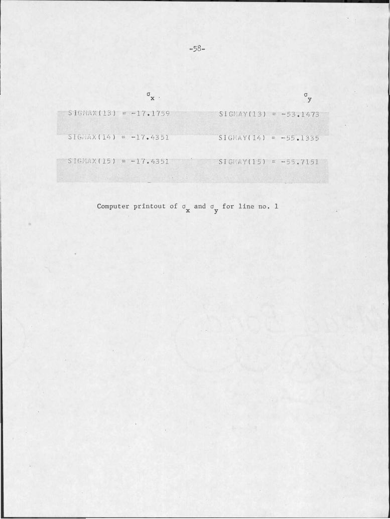
-58-
oX
S IGALiX ( 13) = -17.1759 SIGi:AY(13) = -53
SIGiiAX ( 14 ) = -17.4351 SI GCAY( 14) = -55
SIGnAX(IS) = -17.4351 SI GCAY(I 5) = -55
Computer printout of O^ and for line no. I
ay1473
1335
7151
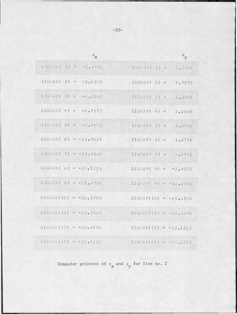
-59-
oX
a IGi ( I ) = -2.4450
SIGMAX ( 2 ) = -3.6385
SIGMAXI 3 ) = -5.0331
SIGMAX( 4 ) = -6.7173
SIGMAXI 5 ) = -8.9991
SIGMAX I 6 ) = -11.9825
SIG AX I 7) = -15.9186
SIGMAX I 8 ) = -18.5215
SIGMAX I 9) = -21.4706
SIGMAX I 10 ) = -22.3780
S IG' .X I 11 ) = -22.2466
SIGMAX(12) = -22.0236
SIGMAXI13) = -22.4116
Computer printout of o
aySlGMAYI I ) - 3.2664
SIGHAYI 2 ) = 4.7573
SIGHAYI 3 ) = 2.3951
SI GMAYI 4) = 2.2865
SIGHAYI 5) = 2.0740
SI GMAYI 6) = 1.0774
SIGHAYI 7 ) = -.4982
SI GMAY I 8) = -2.9523
SIGHAYI 9) = -10.0936
SI GMAY I 10) = -19.6709
SI GMiAYI 11) = -32.5294
SI GMAYI 12) = -42.1228
SI GHAYI13) = -50.2257
for line no. 2
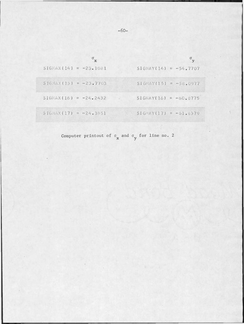
-60-
OX OySIGKAX(14 ) = -23. 3.081 SI GMAY(14) = -54.7707
S IGMAX(15) = -23.7703 SI GHAYd 5 ) = -58.0977
SIGKAX( 16 ) = -24.2432 SI GMAY(16) = -60.8775
SIGKtiX(17) = -24.3851 SIGHAY(IY) = -61.0379
Computer printout of and a for line no. 2
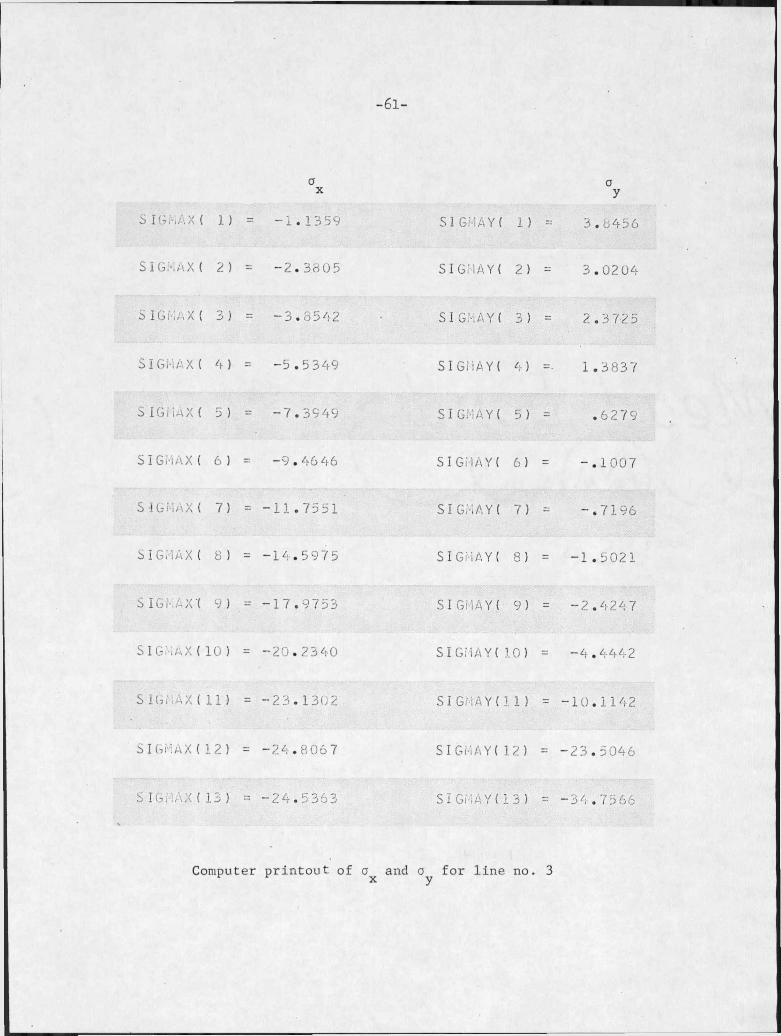
-6l-
OX ayS I (7,-./.X ( I) -1.1359 SlGMAYf I ) = 3.0456
SIGMAXf 2) -2.3805 SIGMAYf 2 ) = 3.0204
SIGMAXf 3) -3.8542 SIGMAYf 3 ) = 2.3725
SIGMAX( 4) -5.5349 SIGMAYf 4) =• 1.3837
SIGiwXf 5) = -7.3949 SIGMAYf 5) = .6279
SIGMAXf 6) —9.46 46 SIGMAYf 6) = -.1007
SIGMAXf 7) -11.7551 SIGMAYf 7) - -.7196
SIGMAXf 8) -14.5975 SIGMAYf 8) = -I.5021
SIGMAXI 9) -17.9753 SIGMAYf 9) = -2.4247
SIGMa X (10 ) -20.2340 SIGMAYf10) = —4.4442
SIGMAX(11) -23.1302 SI GMAYf I I ) = -10.1142
SIGHAXf12) -24.8067 SIGMAYf 12) = -23.5046
S IG. :AX( IS) -24.5363 SI GHAYf13) = -34.7566
Computer printout of a and a for line x y no. 3
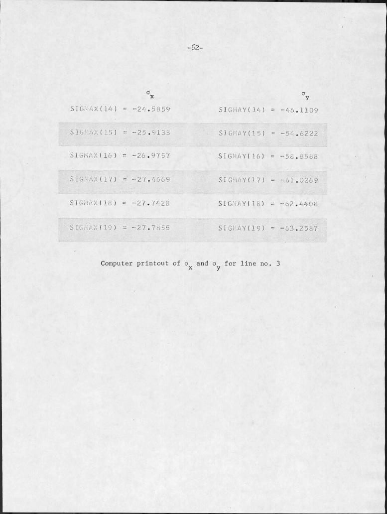
-62-
OX aySIGMAX(14) = -2A.5859 SI GMAY( 14) = — 4-6.1109
SIG',,X (15) = -25.9133 SIGMAY(IS) = -54.6222
SIGMAX(16) = -26.9757 SI GHAY(16) = -58.8588
SIG ;\X(17) = -27.4669 SI GMAY(17) = -61.0269
SIGMAX(IB) = -27.7428 SIGMAYt18) = -62.4408
S IGf .AX( 19) = -27.7855 SIGMAYI19) = -63.2587
Computer printout of a and a for line no. 3
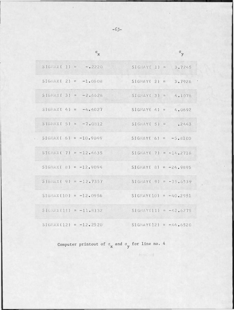
-63-
6IG,:,.X( I) =
SIGHAX( 2) =
SIGrAXI 3) =
SIGiAXt 4) =
SIGhAXt 5) =
SIGMAXt 6) =
SIG ^Xt 7) =
SIGMAX( 8) =
SIGriAXt 9) =
SIGMAX(10) =
SIGMAX( 11 ) =
SI GMAX(12 ) =
Computer
ax
-.2220
-1.0608
-2.6628
-4.4027
-7.0812
-10.9049
-12.4635
-12.9094
-12.7357
-12.0956
-11.8132
-12.2520
SIGMAYt I)
SIGMAYt 2)
SIGMAYt 3)
SIGMAYt 4)
SIGMAYt 5)
SIGMAYt 6)
SIGMAYt 7)
SIGHAYt 8)
SIGHAYt 9)
SIGMAYt10)
SIGMAY(Il)
SIGHAYt12)
y
= 3.7245
= 3.7926
= 4.1076
= 4.0692
= .2443
= -5.8100
= -14.2716
= -24.9895
= -35.6539
= -40.2951
= -42.6275
- — 44.6520
printout of a^ and for line no. 4
-64-
X ySIGrAX( I ) .1370 SIGHAYI I ) = 1.5885
S IGi iAX ( 2) .2397 SI GMAY I 2 ) 2.2315
SIG A X ( 3 ) .1198 SIGHAYI 3) 1.4793
SIGHAX( 4) -.2911 SI GilAYI 4) -.2911
SIG.AX ( 5 I -1.0103 SIGHAYI 5) -3.8843
S IGMAX( 6 ) — 1.6 440 SI GMAYI 6) -9.0796
SIG M A X ( 7 ) -1.7810 SIGHAYI 7) -11.0970
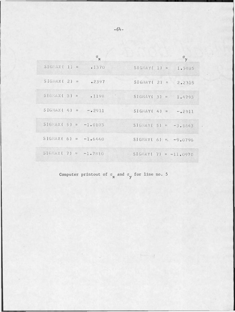
Computer printout of and a^ for line no. 5
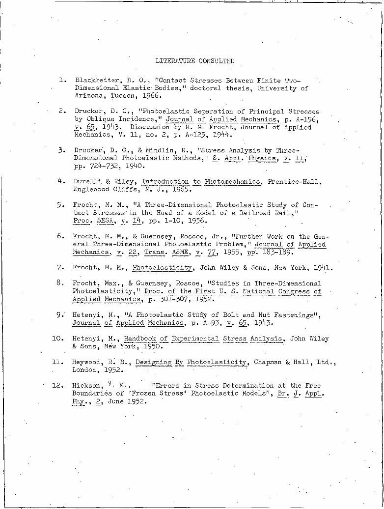
LITERATURE CONSULTED
1. Blackketters D. Q-.. "Contact Stresses Between Finite Two- Dimensional Elastic- Bodies," doctoral thesis, University of Arizona, Tucson, 1966.
2. Drucker, D . C., "Photoelastic Separation of Principal Stresses by Oblique Incidence," Journal of Applied Mechanics, p. A-I56,_v. 65, 19^3* Discussion by M. M. Frocht, Journal of Applied Mechanics, V. 11, no. 2, p. A-125, 1944.
3* Drucker', D. C., & Mindlin, R., "Stress Analysis by Three- Dimensional Photoelastic Methods," S_. Appl. 'Physics, V_. II,PP. 724-732, 1940.
4. Durelli & Riley, Introduction to Photomechanics, Prentice-Hall, Englewood Cliffs, N. J., 196$.
5• Frocht, M. M., "A Three-Dimensional Photoelastic Study of Contact Stresses'in the Head of a Model of a Railroad Rail,"Proc. SESA, y. l4, pp. 1-10, 1956.
6. Frocht, M. M., & Guernsey, Roscoe, Jr., "Further Work on the General Three-Dimensional Photoelastic Problem," Journal of Applied Mechanics, y_. 22, Trans. ASME, y_. 77, 1955, pp« I83-I89.
7- Frocht, M. M., Photoelasticity, John Wiley & Sons, New York, 1941.
8. Frocht, Max., & Guernsey, Roscoe, "Studies in Three-Dimensional Photoelasticity," Proc. of the First U. S_. National Congress of Applied Mechanics, p. 301-307, 1952.
9« Hetenyi, M., "A Photoelastic Study of Bolt and Nut Fastenings", Journal of Applied Mechanics, p. A-93, y.. 65, 1943»
10. Hetenyi, M., Handbook of Experimental Stress Analysis, John Wiley & Sons, New York, 1950.
11. Heywood, R. B., Designing By Photoelasticity, Chapman & Hall, Ltd.,London, 1952. '
Hickson, M., "Errors in Stress Determination, at the FreeBoundaries of 'Frozen Stress' Photoelastic Models", Br. tJ. Appl.Phy., 2_, June 1952.
12.
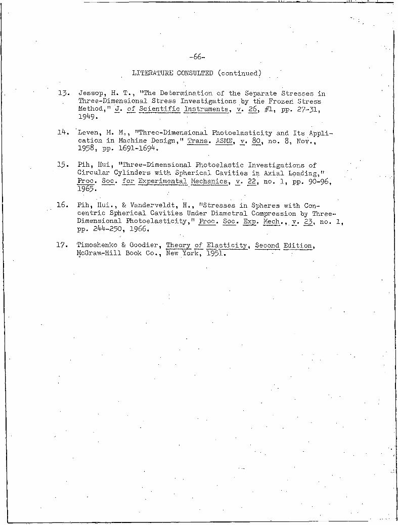
-66-
13. Jessop1 H. T., "The Determination of the Separate Stresses in Three-Dimensional Stress Investigations by the Frozen Stress Method," J. of Scientific Instruments, v. 26, #1, pp. 27-31,1949.
l4« Levenl, M. M,, "Three-Dimensional Photoelasticity and Its Application in Machine Design," Trans. ASME, v. 80, no. 8, Nov.,1958, pp. 1691-1694.
15• Pih, Hui, "Three-Dimensional Photoelastic Investigations of Circular Cylinders with Spherical Cavities in Axial Loading,"Proc. Soc. for Experimental Mechanics, v. 22, no. I, pp. 90-96, 1965.
16. Pih, Hui., & Vanderveldt, H., "Stresses in Spheres with Concentric Spherical Cavities Under Diametral Compression by Three- Dimensional Photoelasticity," Proc. Soc., Exp. Mech., v. 23, no. I, pp. 244-250, 1966.
I?. Timoshenko & Goodier, Theory of Elasticity, Second Edition, McGraw-Hill Book Co., New York, 1951.
LITERATURE CONSULTED (continued)
state WW E=Sin LlWRIES
3 1762 10015432 5
N372 Schafer, D.C.Sch13 A photoelastic incop.2 vegtigation of three"
dimensional contact stresses
f< AM Agggggr
/ X / 7 . 7 J 7 T 7
/V372S c h / 3Q.0p ' 3-
^ o EIh c e ?
Related Documents