A persistence-based Wold-type decomposition for stationary ...

Quantitative Economics 11 (2020), 203–230 1759-7331/20200203

A persistence-based Wold-type decomposition for stationarytime series

Fulvio OrtuDepartment of Finance, Università Bocconi and IGIER

Federico SeverinoDépartement de Finance, Assurance et Immobilier, FSA, Université Laval and Department of Economics,

USI Lugano

Andrea TamoniDepartment of Finance and Economics, Rutgers Business School

Claudio TebaldiDepartment of Finance, Università Bocconi, IGIER, and Baffi-CAREFIN

This paper shows how to decompose weakly stationary time series into the sum,across time scales, of uncorrelated components associated with different degreesof persistence. In particular, we provide an Extended Wold Decomposition basedon an isometric scaling operator that makes averages of process innovations.Thanks to the uncorrelatedness of components, our representation of a time se-ries naturally induces a persistence-based variance decomposition of any weaklystationary process. We provide two applications to show how the tools developedin this paper can shed new light on the determinants of the variability of economicand financial time series.Keywords. Wold decomposition, temporal aggregation, persistence heterogene-ity, forecasting.

JEL classification. C18, C22, C50.

1. Introduction

This paper formalizes the idea that a stationary time series decomposes into the sum oforthogonal layers with heterogeneous levels of durations. Notably, our representation is

Fulvio Ortu: [email protected] Severino: [email protected] Tamoni: [email protected] Tebaldi: [email protected] thank T. Andersen, S. Cerreia-Vioglio, M. Chernov, F. Corsi, R. Gallant, L.P. Hansen, M. Henry, M. Mar-cellino, G. Primiceri, P. Reggiani, E. Renault, L. Sala, E. Sentana, P. Veronesi, and M. Watson, and participantsat the 2017 NBER/NSF Time Series Conference at Kellogg, University of Chicago, 11th World Congress ofthe Econometric Society in Montréal, 8th International Conference on CFE in Pisa, Università degli Studidi Udine, 11th CSEF-IGIER Symposium on Economics and Institutions in Capri, XLI AMASES Meeting inCagliari, and 11th Annual SoFiE Conference in Lugano for helpful suggestions.

© 2020 The Authors. Licensed under the Creative Commons Attribution-NonCommercial License 4.0.Available at http://qeconomics.org. https://doi.org/10.3982/QE994

204 Ortu, Severino, Tamoni, and Tebaldi Quantitative Economics 11 (2020)

obtained in the time-domain. Thus, although it shares many of the insights of frequencydomain methods, our approach is well suited for predictive analysis, where time adap-tation and localization in both time and frequency, are crucial.

Our main result shows how to represent a stationary time series as a sum of orthogo-nal components each one characterized by a specific level of persistence (or scale). Ournovel representation produces an Extended Wold Decomposition in which each com-ponent at scale j is an infinite moving average driven by a sequence of uncorrelatedinnovations that are located on a time grid whose unit spacing is 2j the original unitgrid.

As a byproduct of the orthogonality of components, our approach naturally providesa variance decomposition of the time series. Differently from the traditional principalcomponent analysis (PCA) approach, each component in our analysis is associated witha specific scale, a fact that comes to aid when one has to provide an economic interpreta-tion of the key driving factors. Indeed, different economic phenomena most likely oper-ate at different frequencies, for example, price movements can be related to announce-ments of macroeconomic conditions and corporate activity at the short-end of spec-trum, to political cycles at the medium-end, to technological and demographic changesat the long-end, and to uncertainty regarding exhaustible energy resources and climatechange at the very long-end (see, e.g., the literature review in Ortu, Tamoni, and Tebaldi(2013)). Therefore, by being informative about the duration of the fluctuation most rel-evant for the time series variability, our approach sheds light on the potential economicmechanism driving the time series.

Our extended Wold decomposition also provides an interpretation of the notion ofpersistence for stationary processes. Indeed, our construction exploits the isometry of ascaling operator that smooths the original time series by making successive averages ofthe process innovations. Such procedure implicitly defines an index j that we dub scaleor degree of persistence. In fact, a shock at scale j has, by construction, a mean reversiontime ranging between 2j−1 and 2j , and its spectrum is localized in the correspondingband of frequencies.

Whereas our first main result (Theorem 1) shows how to decompose and analyze atime series in terms of its persistent components, our second main result (Theorem 2)shows how to build a stationary process starting from uncorrelated components withheterogeneous degrees of persistence. This second result is important as it offers a newfamily of (data generating) processes suitable to capture phenomena evolving over timescales of different length (or frequency). Interestingly, Robinson (1978) and Granger(1980) proposed contemporaneous aggregation of individual, random coefficient AR(1)processes as a mechanism that leads to long memory. Relying on Theorem 2, the simu-lations in Section 2.2.1 show that a finite (in fact as small as two) sum of autoregressiveprocesses with fixed autoregressive coefficients is able to generate hyperbolically decay-ing autocorrelation functions as long as the processes evolve over different time scales(e.g., monthly and annual). On the technical side, the proof of Theorem 2 highlights thatthe reconstructed time series is stationary because each scale-specific shock is assumedto be a weighted linear combination of underlying innovations.

We provide two applications to show the relevance of our decomposition.

Quantitative Economics 11 (2020) A persistence-based Wold-type decomposition 205

In the first empirical application, we investigate the drivers of realized volatility incurrency markets. We show that three components operating over semiannual, annual,and biannual frequencies account for a substantial fraction of variability of daily realizedvariance. A forecasting model using only these three components performs well relativeto the Heterogeneous Autoregressive model (HAR) model of Corsi (2009). Interestingly,also the HAR model relies on three regressors—namely daily, weekly, and monthly real-ized volatility series—to forecast daily volatility. Both our model based on Wold compo-nents and the HAR model provide evidence that volatility reflects the aggregate impactof processes evolving over different time scales. However, our analysis further shows thatthe daily, weekly, and monthly components of Corsi (2009) indeed proxy for phenom-ena occurring over longer time scales in between a half-year and two years. Moreover, ifone adopts the “Heterogeneous Market Hypothesis” of Müller, Dacorogna, Dave, Pictet,Olsen, and Ward (1993) where each volatility component is generated by the actions ofspecific types of market participants, then our analysis is informative about the horizonsof such investors.

In the second application, we employ our extended Wold decomposition to investi-gate the relation between yields and bond returns. Our analysis shows that the extendedWold decomposition is able to detect yield cycles useful for bond predictability. We showthat a model based on a high frequency component of the level and a low frequencycomponent of the slope attains a fit similar to the Cieslak and Povala (2015) model. Thelatter detrends the level of the yield curve using an inflation trend. Despite the same fit,the two models call for different economic interpretation. In our analysis, the factorsdriving bond returns are orthogonal, and hence economic theory needs to explain thehigh- and low-frequency cycles in the yield curve only. In the Cieslak and Povala (2015)framework, the factors are negatively correlated so that economic theory needs to ex-plain not only the (detrended) level and slope, but also their relative value.

In order to clarify positioning, we discuss how our results relate to some existingapproaches. Ortu, Tamoni, and Tebaldi (2013) proposed to use multiresolution analysisto study the asset prices reaction in dynamic economies hit by shocks of heterogeneousdurations. The authors show that exposure to specific consumption components (ratherthan raw consumption) is a source of priced risk and it can explain the level of the equitypremium. Bandi, Perron, Tamoni, and Tebaldi (2019) show that the empirical relationbetween future excess market returns and past economic uncertainty is hump-shaped,that is, the R-squared (R2) values reach their peak at 16 years and the structure of the R2s,before and after, is roughly tent-shaped. These authors show that classical predictivesystems imply restrictions across scales which are inconsistent with the hump-shapedrelation between uncertainty and returns. To justify their findings formally, Bandi et al.(2019) introduced a novel modeling framework in which predictability is specified as aproperty of the components of excess market returns and economic uncertainty. Theextended Wold decomposition formalized in this paper is used, in their framework, tomodel predictability across scales and justify extraction of the components. Finally, theextended Wold decomposition proves also useful in the context of cross-sectional assetpricing. Bandi, Lo, Chaudhuri, and Tamoni (2019) employ the extended Wold decom-position to introduce novel spectral factor models in which systematic risk is allowed

206 Ortu, Severino, Tamoni, and Tebaldi Quantitative Economics 11 (2020)

(without being forced) to vary across different frequencies. The authors show that spec-tral factors models lead to portfolios with lower out-of-sample variance relative to port-folios constructed under the assumption that risk is constant across frequencies.

The present paper shows that a stationary time series can be described as thesum of uncorrelated components with different levels of persistence. A component atlevel of persistence j admits a classical Wold decomposition in terms of innovationsthat are moving averages of the original innovations and are localized on a time gridwhose unit is 2j units of the original observation grid. The coarsening of the grid wherelow-frequency shocks are located is closely related to the frequency-domain procedureadopted by Müller and Watson (2008) and Müller and Watson (2017), where long-runsample information is isolated using a small number of low-frequency trigonometricweighted averages which, in turn, can be used to conduct inference about long-run vari-ability and covariability. Differently from them, our resulting representation uses infor-mation only up to time t, and thus, it does not suffer from the look-ahead bias typical ofa two-sided frequency representation.

Our persistence-based Wold-type representation lays the foundation for processesthat have been proposed in the literature to capture the long-range dependence exhib-ited by many financial time series, such the Heterogeneous Information Arrivals processsuggested by Andersen and Bollerslev (1997), the Markov-Switching Multifractal work byCalvet and Fisher (2007), the Heterogeneous Autoregressive Model of Realized Volatility(HAR-RV) developed by Corsi (2009), the component-GARCH models of Engle and Lee(1999), and the Spline-Garch framework of Engle and Rangel (2008).

Our decomposition into components with different persistence levels is additive.This is in contrast with the MIDAS (Mi(xed) Da(ta) S(ampling)) regressions developedin Ghysels, Santa-Clara, and Valkanov (2004) and Ghysels, Santa-Clara, and Valkanov(2006), where the smoothing coefficients interact multiplicatively in a way that makes itdifficult to isolate the effects of each components.

The rest of the paper is organized as follows. Section 2 presents the theoretical re-sults of the paper. We start with a finite-dimensional example to illustrate the key stepsneeded to decompose a zero-mean, purely nondeterministic process into the sum ofuncorrelated components associated with different levels of persistence. In Section 2.1,we introduce our isometric scaling operator, we derive the extended Wold decomposi-tion, and we analyze its main properties. We also look at our decomposition from thestandpoint of spectral analysis and show that our operator acts as a low-pass filter. Wedevote Section 2.2 to establish the converse result, that is, how to compute the mov-ing average representation of a weakly stationary time series that is obtained by sum-ming heterogeneous components at different scales. In that section, we also illustratethe reconstruction theorem by means of an example. Section 2.3 describes the relationbetween the extended Wold decomposition and the multiresolution-based decomposi-tion proposed in Ortu, Tamoni, and Tebaldi (2013). In particular, we contrast, for a fixedlevel of persistence, the spectrum of the components obtained from our scaling oper-ator with that generated by multiresolution analysis. Section 3 describes two empiricalapplications of the extended Wold decomposition to realized volatility and bond yields.Section 4 concludes. All proofs are in the Online Supplemental Material (Ortu, Severino,Tamoni, and Tebaldi (2020)).

Quantitative Economics 11 (2020) A persistence-based Wold-type decomposition 207

2. The extended Wold decomposition

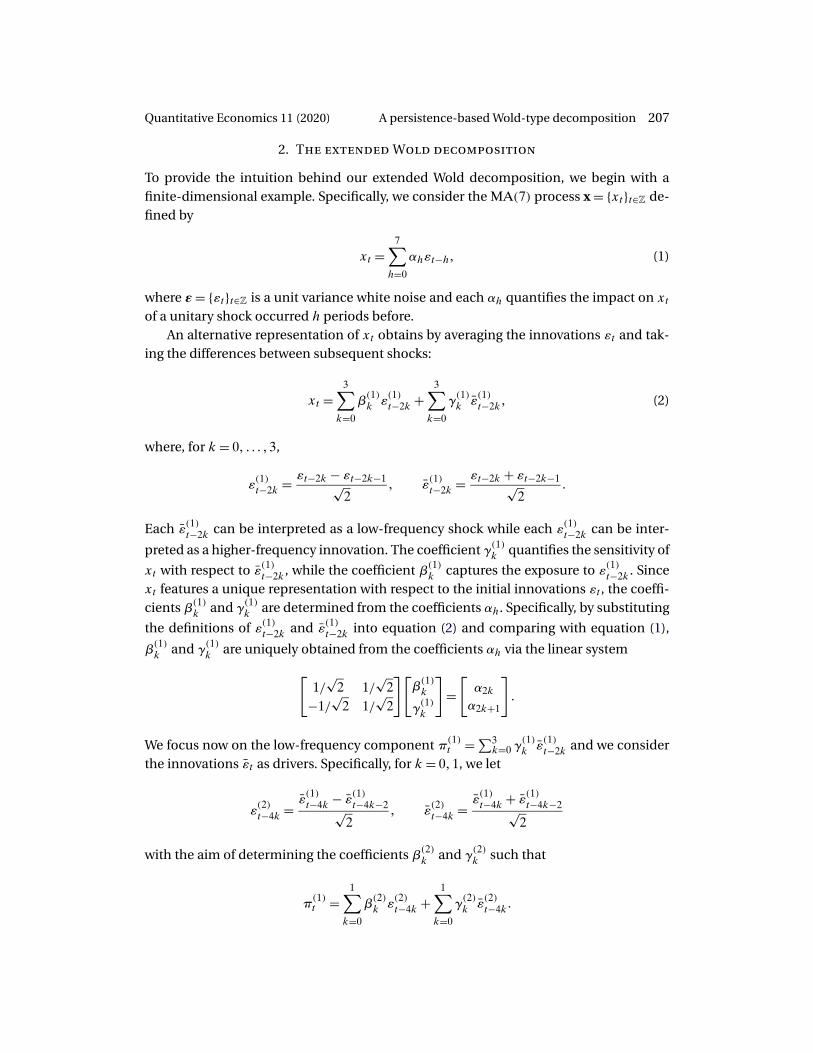
To provide the intuition behind our extended Wold decomposition, we begin with afinite-dimensional example. Specifically, we consider the MA(7) process x = {xt}t∈Z de-fined by

xt =7∑

h=0

αhεt−h� (1)

where ε = {εt}t∈Z is a unit variance white noise and each αh quantifies the impact on xtof a unitary shock occurred h periods before.

An alternative representation of xt obtains by averaging the innovations εt and tak-ing the differences between subsequent shocks:

xt =3∑

k=0

β(1)k ε(1)t−2k +

3∑k=0

γ(1)k ε(1)t−2k� (2)

where, for k= 0� � � � �3,

ε(1)t−2k = εt−2k − εt−2k−1√2

� ε(1)t−2k = εt−2k + εt−2k−1√2

�

Each ε(1)t−2k can be interpreted as a low-frequency shock while each ε(1)t−2k can be inter-

preted as a higher-frequency innovation. The coefficient γ(1)k quantifies the sensitivity of

xt with respect to ε(1)t−2k, while the coefficient β(1)k captures the exposure to ε(1)t−2k. Since

xt features a unique representation with respect to the initial innovations εt , the coeffi-cients β(1)

k and γ(1)k are determined from the coefficients αh. Specifically, by substituting

the definitions of ε(1)t−2k and ε(1)t−2k into equation (2) and comparing with equation (1),

β(1)k and γ

(1)k are uniquely obtained from the coefficients αh via the linear system

[1/

√2 1/

√2

−1/√

2 1/√

2

][β(1)k

γ(1)k

]=

[α2kα2k+1

]�

We focus now on the low-frequency component π(1)t = ∑3

k=0 γ(1)k ε

(1)t−2k and we consider

the innovations εt as drivers. Specifically, for k= 0�1, we let

ε(2)t−4k = ε(1)t−4k − ε

(1)t−4k−2√

2� ε(2)t−4k = ε

(1)t−4k + ε

(1)t−4k−2√

2

with the aim of determining the coefficients β(2)k and γ(2)

k such that

π(1)t =

1∑k=0

β(2)k ε(2)t−4k +

1∑k=0

γ(2)k ε(2)t−4k�

208 Ortu, Severino, Tamoni, and Tebaldi Quantitative Economics 11 (2020)

We do so by solving, for k= 0�1, the linear system[1/

√2 1/

√2

−1/√

2 1/√

2

][β(2)k

γ(2)k

]=

[γ(1)

2k

γ(1)2k+1

]�

As a final step, we concentrate on the term π(2)t = ∑1

k=0 γ(2)k ε(2)t−4k generated by the

shocks ε(2)t . Similar to the previous construction, we obtain

π(2)t = β

(3)0 ε

(3)t + γ

(3)0 ε

(3)t

with

ε(3)t = ε(2)t − ε(2)t−4√2

� ε(3)t = ε(2)t + ε(2)t−4√2

�

Accordingly, β(3)0 and γ

(3)0 constitute the unique solution of the system

[1/

√2 1/

√2

−1/√

2 1/√

2

][β(3)

0

γ(3)0

]=

[γ(2)

0

γ(2)1

]�

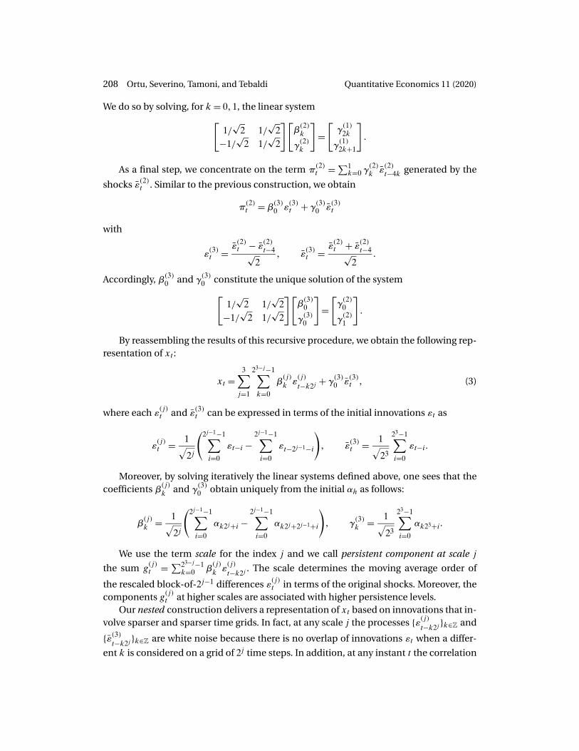
By reassembling the results of this recursive procedure, we obtain the following rep-resentation of xt :

xt =3∑

j=1

23−j−1∑k=0

β(j)k ε

(j)

t−k2j + γ(3)0 ε

(3)t � (3)

where each ε(j)t and ε(3)t can be expressed in terms of the initial innovations εt as

ε(j)t = 1√

2j

(2j−1−1∑i=0

εt−i −2j−1−1∑i=0

εt−2j−1−i

)� ε(3)t = 1√

23

23−1∑i=0

εt−i�

Moreover, by solving iteratively the linear systems defined above, one sees that thecoefficients β(j)

k and γ(3)0 obtain uniquely from the initial αh as follows:

β(j)k = 1√

2j

(2j−1−1∑i=0

αk2j+i −2j−1−1∑i=0

αk2j+2j−1+i

)� γ(3)

k = 1√23

23−1∑i=0

αk23+i�

We use the term scale for the index j and we call persistent component at scale j

the sum g(j)t = ∑23−j−1

k=0 β(j)k ε

(j)

t−k2j . The scale determines the moving average order of

the rescaled block-of-2j−1 differences ε(j)t in terms of the original shocks. Moreover, the

components g(j)t at higher scales are associated with higher persistence levels.Our nested construction delivers a representation of xt based on innovations that in-

volve sparser and sparser time grids. In fact, at any scale j the processes {ε(j)t−k2j }k∈Z and

{ε(3)t−k2j }k∈Z are white noise because there is no overlap of innovations εt when a differ-

ent k is considered on a grid of 2j time steps. In addition, at any instant t the correlation

Quantitative Economics 11 (2020) A persistence-based Wold-type decomposition 209

between any ε(j)t and ε

(l)t with j �= l is null. Each ε

(j)t is also uncorrelated with ε

(3)t . There-

fore, equation (3) provides a decomposition of xt in terms of a linear combination ofincreasingly persistent components that are orthogonal.

Interestingly, the scale-specific shocks ε(j)t and ε

(3)t can be seen as the application

of the discrete Haar transform to the sequence of the original innovations εt (see, forinstance, Addison (2002)). The same property holds for the coefficients β

(j)k and γ

(3)0 ,

which are obtained from the discrete Haar transform of the sequence of coefficients αh.Hence, we can readily compute β

(j)k and γ

(3)0 from the original MA representation of xt .

In light of this example, we ask whether it is possible to generalize the decompositionof eq. (3) in two main directions. First, we want to deal with MA processes of any order.By the classical Wold decomposition theorem, this permits to analyze any weakly sta-tionary time series. Second, we want to allow for a potentially infinite number of scalesin order to reduce as much as possible the magnitude of the term γ

(3)0 ε

(3)t so to obtain a

univocal persistence-based decomposition. We do this in the next section.

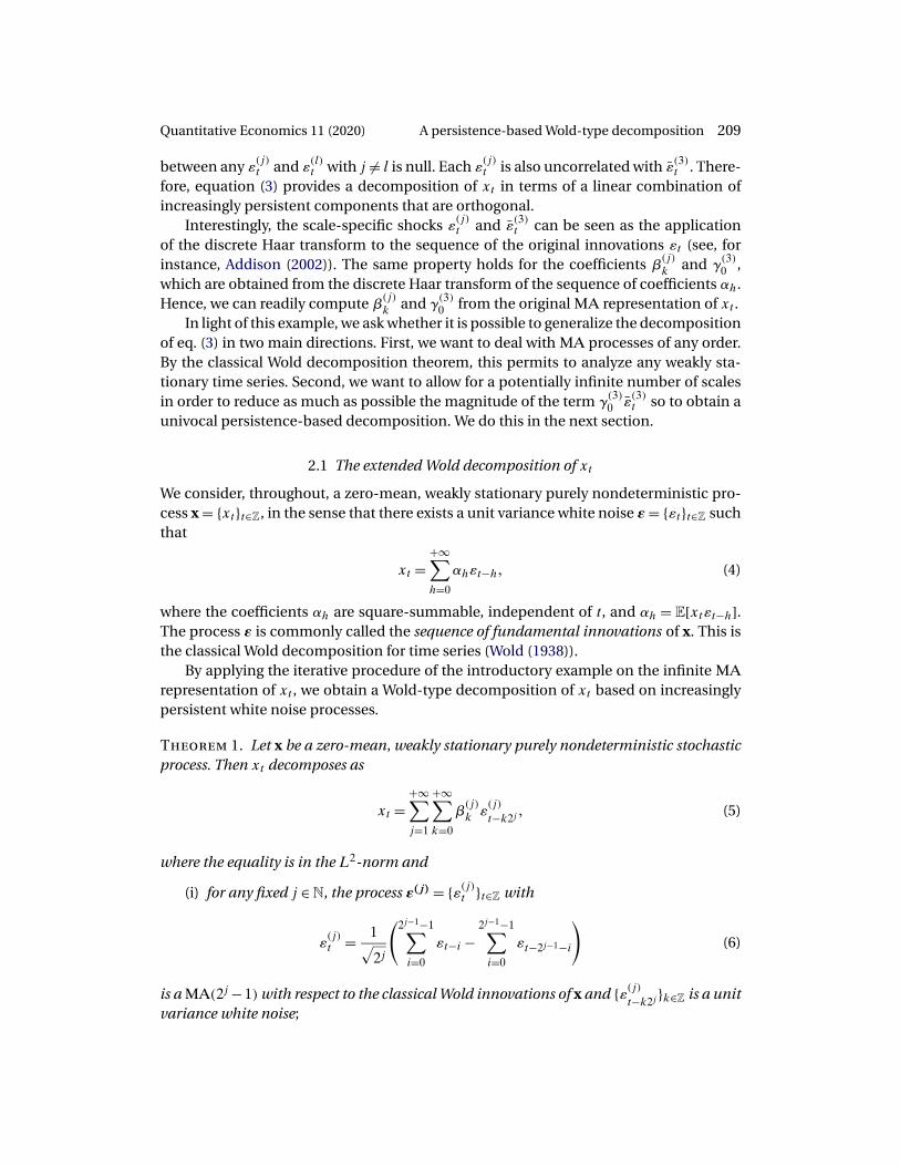
2.1 The extended Wold decomposition of xt

We consider, throughout, a zero-mean, weakly stationary purely nondeterministic pro-cess x = {xt}t∈Z, in the sense that there exists a unit variance white noise ε= {εt}t∈Z suchthat

xt =+∞∑h=0

αhεt−h� (4)

where the coefficients αh are square-summable, independent of t, and αh = E[xtεt−h].The process ε is commonly called the sequence of fundamental innovations of x. This isthe classical Wold decomposition for time series (Wold (1938)).

By applying the iterative procedure of the introductory example on the infinite MArepresentation of xt , we obtain a Wold-type decomposition of xt based on increasinglypersistent white noise processes.

Theorem 1. Let x be a zero-mean, weakly stationary purely nondeterministic stochasticprocess. Then xt decomposes as

xt =+∞∑j=1

+∞∑k=0

β(j)k ε

(j)

t−k2j � (5)

where the equality is in the L2-norm and

(i) for any fixed j ∈N, the process ε(j) = {ε(j)t }t∈Z with

ε(j)t = 1√

2j

(2j−1−1∑i=0

εt−i −2j−1−1∑i=0

εt−2j−1−i

)(6)

is a MA(2j −1) with respect to the classical Wold innovations of x and {ε(j)t−k2j }k∈Z is a unit

variance white noise;

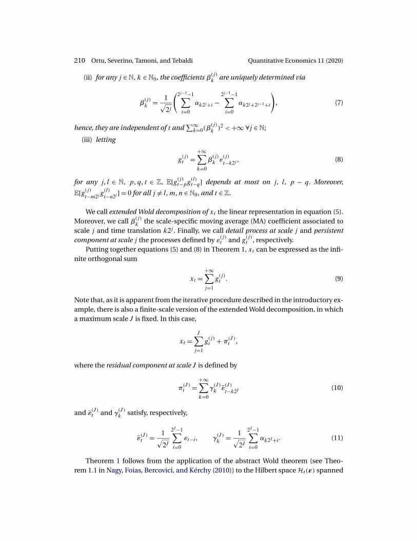
210 Ortu, Severino, Tamoni, and Tebaldi Quantitative Economics 11 (2020)

(ii) for any j ∈N, k ∈N0, the coefficients β(j)k are uniquely determined via

β(j)k = 1√

2j

(2j−1−1∑i=0

αk2j+i −2j−1−1∑i=0

αk2j+2j−1+i

)� (7)

hence, they are independent of t and∑∞

k=0(β(j)k )2 < +∞ ∀j ∈N;

(iii) letting

g(j)t =

+∞∑k=0

β(j)k ε

(j)

t−k2j � (8)

for any j� l ∈ N, p�q� t ∈ Z, E[g(j)t−pg(l)t−q] depends at most on j, l, p − q. Moreover,

E[g(j)t−m2j g

(l)

t−n2l] = 0 for all j �= l, m�n ∈N0, and t ∈ Z.

We call extended Wold decomposition of xt the linear representation in equation (5).Moreover, we call β(j)

k the scale-specific moving average (MA) coefficient associated toscale j and time translation k2j . Finally, we call detail process at scale j and persistentcomponent at scale j the processes defined by ε

(j)t and g

(j)t , respectively.

Putting together equations (5) and (8) in Theorem 1, xt can be expressed as the infi-nite orthogonal sum

xt =+∞∑j=1

g(j)t � (9)

Note that, as it is apparent from the iterative procedure described in the introductory ex-ample, there is also a finite-scale version of the extended Wold decomposition, in whicha maximum scale J is fixed. In this case,

xt =J∑

j=1

g(j)t +π(J)

t �

where the residual component at scale J is defined by

π(J)t =

+∞∑k=0

γ(J)k ε(J)

t−k2J (10)

and ε(J)t and γ

(J)k satisfy, respectively,

ε(J)t = 1√2J

2J−1∑i=0

εt−i� γ(J)k = 1√

2J

2J−1∑i=0

αk2J+i� (11)

Theorem 1 follows from the application of the abstract Wold theorem (see Theo-rem 1.1 in Nagy, Foias, Bercovici, and Kérchy (2010)) to the Hilbert space Ht (ε) spanned

Quantitative Economics 11 (2020) A persistence-based Wold-type decomposition 211

by the sequence of fundamental innovations {εt−k}k∈N0 :

Ht (ε) ={+∞∑k=0

akεt−k :+∞∑k=0

a2k < +∞

}�

In words, Ht (ε) is the space of infinite moving averages generated by ε. The AbstractWold Theorem provides an orthogonal decomposition of Ht (ε) by iteratively applyingan isometric linear operator that generalizes the recursive procedure of the introductoryexample. Specifically, in our case we define the scaling operator R : Ht (ε)−→ Ht (ε) by

R :+∞∑k=0

akεt−k �−→+∞∑k=0

ak√2(εt−2k + εt−2k−1) =

+∞∑k=0

a k2 √2εt−k� (12)

where · associates any real number c with the integer c = max{n ∈ Z : n ≤ c}. Thescaling operator is well-defined, linear, and isometric on Ht (ε). As a result, Ht (ε) de-composes into the direct sum Ht (ε) = ⊕∞

j=0 RjLRt , where LR

t is the orthogonal comple-ment of RHt (ε). From the classical Wold decomposition, xt belongs to Ht (ε) and so thedecomposition into uncorrelated components of equation (9) follows from projecting xton the orthogonal subspaces.1

Property (iii) in Theorem 1 concerns the relation among the components g(j)t at dif-

ferent layers of persistence. When t is fixed, the variables g(j)t and g(l)t , with j �= l, are un-correlated. Besides, the uncorrelation involves also shifted variables g

(j)

t−m2j and g(l)t−n2l

,

for any m�n ∈ Z, where the time translation is proportional to 2j and 2l, respectively. Ingeneral, the covariance between g

(j)t−p and g

(l)t−q depends at most on the scales j, l, and

on the difference p− q.The orthogonality of the persistent components is a key property since it allows for

a decomposition of the total variance of xt across persistence levels:

var(xt)=+∞∑j=1

var(x(j)t

) =+∞∑j=1

+∞∑k=0

(β(j)k

)2�

Thus, the extended Wold decomposition induces a persistence-based variance decom-position of any weakly stationary process, thanks to the uncorrelatedness of compo-nents ensured by the abstract Wold theorem. The key novelty is that our persistence-based variance decomposition speaks about the role of both time and frequency in theevaluation of the impact of economic shocks, whereas classical time-series methods,like principal component analysis, find it often onerous to disentangle the two dimen-sions.

We remark that it is also possible to build an extended Wold decomposition based ontime grids of Nj steps instead of 2j . This orthogonal decomposition exploits an isometricoperator that generalizes R by averaging N subsequent innovations instead of just 2.

1Interestingly, the same logic underlies the classical Wold decomposition, that can be derived by em-ploying the lag operator as isometry. See Severino (2016).

212 Ortu, Severino, Tamoni, and Tebaldi Quantitative Economics 11 (2020)

Details can be found in the Addendum available upon request or on the website fromthe authors.

Importantly, the approach that exploits the abstract Wold theorem and the isometricscaling operator to identify the persistent components generalizes to stationary multi-variate processes. In a nutshell, Theorem 1 continues to hold even when x, ε and allε(j) are m-dimensional processes, so that αh and β

(j)k are m×m matrices of coefficients.

Therefore, any multivariate stationary process admits a decomposition of the type

xt =+∞∑j=1

+∞∑k=0

β(j)k ε

(j)

t−k2j �

where square-summability is ensured by the convergence of∑∞

k=0 Tr(β(j)k β

(j)k

′), the trace

of the matrix β(j)k β

(j)k

′. We refer the reader interested in the technical details to Cerreia-

Vioglio, Ortu, Severino, and Tebaldi (2017).Finally, we look at our decomposition from the standpoint of spectral analysis.

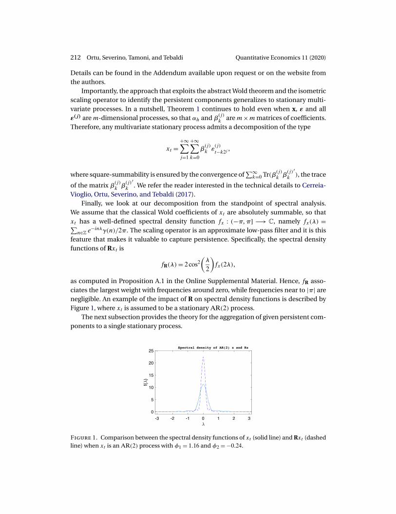
We assume that the classical Wold coefficients of xt are absolutely summable, so thatxt has a well-defined spectral density function fx : (−π�π] −→ C, namely fx(λ) =∑

n∈Z e−inλγ(n)/2π. The scaling operator is an approximate low-pass filter and it is thisfeature that makes it valuable to capture persistence. Specifically, the spectral densityfunctions of Rxt is

fR(λ)= 2 cos2(λ

2

)fx(2λ)�

as computed in Proposition A.1 in the Online Supplemental Material. Hence, fR asso-ciates the largest weight with frequencies around zero, while frequencies near to |π| arenegligible. An example of the impact of R on spectral density functions is described byFigure 1, where xt is assumed to be a stationary AR(2) process.

The next subsection provides the theory for the aggregation of given persistent com-ponents to a single stationary process.

Figure 1. Comparison between the spectral density functions of xt (solid line) and Rxt (dashedline) when xt is an AR(2) process with φ1 = 1�16 and φ2 = −0�24.

Quantitative Economics 11 (2020) A persistence-based Wold-type decomposition 213

2.2 Reconstructing a time series from its components

This subsection investigates the converse of our extended Wold decomposition: oncethe dynamics are given at various time scales, what can we say about the resulting pro-cess x, built by summing up such components?

Given the dynamics at different time scales, we want to recover the whole processx = {xt}t∈Z. To make the sum of components feasible, we assume a common innovationprocess ε = {εt}t∈Z. In fact, while MA processes may have multiple representations thatinvolve different innovations, considering MA processes driven by the same source ofrandomness has the advantage that the sum of such time series is still based on thesame random shocks.

At each scale j ∈ N, we define the detail process ε(j) = {ε(j)t }t∈Z as an MA(2j − 1)driven by the underlying innovations ε. More precisely, we assume that

ε(j)t =

2j−1∑i=0

δ(j)i εt−i

for some real coefficients δ(j)i . Next, we consider the processes g(j) = {g(j)t }t∈Z associated

with level of persistence j. We build these processes in a way that on the time grids S(j)t ={t − k2j : k ∈N0} they are well-defined MA(∞) with respect to ε(j). In particular, for anygiven j, we assume that there exists a sequence of coefficients {β(j)

k }k∈N0 such that

+∞∑j=1

+∞∑h=0

(β(j)

h

2jδ

(j)

h−2j h

2j)2

<+∞� (13)

Then, for any t, we define the variables

g(j)t =

+∞∑k=0

β(j)k ε

(j)

t−k2j

and, in addition, we assume

E[g(j)

t−m2j g(l)

t−n2l] = 0 ∀j �= l�∀m�n ∈N0�∀t ∈ Z� (14)

While Condition (13) involves the interaction of the coefficients β(j)k and δ

(j)i , it is

interesting to discuss two special cases in which Condition (13) holds by imposing re-strictions separately on β

(j)k and δ

(j)i .

First, consider the special case of Haar coefficients, that is,

δ(j)i =

⎧⎪⎪⎪⎨⎪⎪⎪⎩

1√2j

if i ∈ {0� � � � �2j−1 − 1}�

− 1√2j

if i ∈ {2j−1� � � � �2j − 1}�(15)

214 Ortu, Severino, Tamoni, and Tebaldi Quantitative Economics 11 (2020)

In this case, Condition (13) translates into the standard square-summability of the coef-ficients β(j)

k , that is,

+∞∑j=1

+∞∑k=0

(β(j)k

)2<+∞�

In addition, Condition (14) is also satisfied as a consequence of the orthogonal structurediscussed in Section 2.1.

Second, one can assume that the coefficients δ(j)i are uniformly bounded over j ∈ N

and i = 1� � � �2j , and require that

+∞∑j=1

2j+∞∑k=0

(β(j)k

)2<+∞�

so that Condition (13) holds once again. In this case, the condition on the coefficientsδ(j)i is weaker, while the square-summability of the β

(j)k is more restrictive.

The following theorem states the properties of the process x obtained by summingthe components g(j) over all the scales j ∈N when Conditions (13) and (14) hold.

Theorem 2. Let ε = {εt}t∈Z be a unit variance white noise process. For any j ∈ N, define

the detail process ε(j) = {ε(j)t }t∈Z as

ε(j)t =

2j−1∑i=0

δ(j)i εt−i�

with δ(j)i ∈ R for i = 0� � � � �2j − 1, and consider a stochastic process g(j) = {g(j)t }t∈Z such

that there exists a sequence of real coefficients {β(j)k }k∈N0 so that Conditions (13) and (14)

are satisfied. Then the process x = {xt}t∈Z defined by

xt =+∞∑j=1

g(j)t

is zero-mean, weakly stationary purely nondeterministic and

xt =+∞∑h=0

αhεt−h with αh =+∞∑j=1

β(j)

h

2jδ

(j)

h−2j h

2j ∀h ∈N0� (16)

The theorem provides the moving average representation, with respect to the inno-vations εt , of the process x built via the aggregation of persistent components. In casethe shocks εt are the classical Wold innovations of x, Theorem 2 supplies the classicalWold decomposition of xt , starting from its persistence-based representation. As a con-sequence, it constitutes a converse result of Theorem 1.

Quantitative Economics 11 (2020) A persistence-based Wold-type decomposition 215

Note that, when the Haar coefficients are employed, the classical impulse responsescan be retrieved via

αh =+∞∑j=1

1√2jβ(j)

h

2jχ

(j)(h)�

where

χ(j)(h) =

⎧⎪⎪⎨⎪⎪⎩

−1 if 2j h2j

∈ {h− 2j + 1� � � � �h− 2j−1}�

1 if 2j h2j

∈ {h− 2j−1 + 1� � � � �h}�

2.2.1 An illustrative example of the reconstruction theorems Next, we provide a simpleexample of a multiscale construction of a stationary process. We consider a two-scaleprocess given by the sum of a fast evolving autoregressive process and a second, morepersistent autoregressive process evolving on a coarser time scale. We show by means ofa numerical example that different choices of parameters have different impacts on theshort and long lags of the ACF of the resulting process.

Given a common innovation process ε = {εt}t∈Z, we let the coefficients δ(j)i in The-

orem 2 be the Haar coefficients of equation (15). We start from two weakly stationarypurely nondeterministic time series, x = {xt}t∈Z and y = {yt}t∈Z, defined by two fami-lies of scale-specific moving average coefficients: {β(j)

x�k}j�k and {β(j)y�k}j�k with j ∈ N and

k ∈N0.We assume the scale-specific moving average coefficients of xt to be

β(j)x�k = ρk2j

x√2j

(1 − ρ2j−1

x

)2

1 − ρx� j ∈N�k ∈N0�

that is, the extended Wold coefficients of a weakly stationary AR(1) process with param-eter ρx, with |ρx| < 1.

We now fix a scale J and we define the scale-specific coefficients of yt by settingβ(j)y�k = 0 if j = 0� � � � � J and

β(j)y�k = ρk2j−J

y√2j−J

(1 − ρ2j−J−1

y

)2

1 − ρy

if j ≥ J + 1, with |ρy | < 1. A simple comparison with β(j)x�k shows that the coefficients β(j)

y�k

identify the autoregressive process y defined on the grid S(J)t = {t − k2J : k ∈N0} by

yt =+∞∑k=0

ρky ε(J)t−k2J �

where

ε(J)t = 1√2J

2J−1∑i=0

εt−i

216 Ortu, Severino, Tamoni, and Tebaldi Quantitative Economics 11 (2020)

denotes the unit variance white noise ε(J) = {ε(J)t−k2J }k∈Z. In contrast with x, which is a

standard AR(1) process, we call y an AR(1) process with horizon 2J . To enhance inter-

pretation, one can think of x as a daily process, while y is a time series acting on longer

lags (e.g., monthly, yearly, . . . ), depending on the choice of J.

By construction, the scale-specific moving average coefficients of z = {zt}t∈Z are the

sum of the extended Wold coefficients of x and y, that is, β(j)z�k = β

(j)x�k +β

(j)y�k for any j ∈N,

k ∈ N0. It is readily checked that all the conditions of Theorem 2 are satisfied. Therefore,

z is weakly stationary and purely nondeterministic. Note that while the sum of two au-

toregressive processes with different horizons is not necessarily stationary, the structure

of the shocks at different scales required by Theorem 2 ensures that this holds true in

this case. Hereafter, we plot the ACF of z for some choices of the parameters ρx, ρy and

of the scale J.

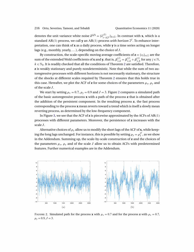
We start by setting ρx = 0�7, ρy = 0�9 and J = 3. Figure 2 compares a simulated path

of the basic autoregressive process x with a path of the process z that is obtained after

the addition of the persistent component. In the resulting process z� the fast process

corresponding to the process x mean reverts toward a trend which is itself a slowly mean

reverting process, as determined by the low-frequency component.

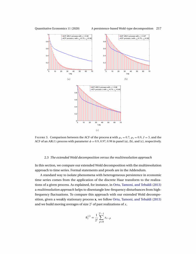
In Figure 3, we see that the ACF of z is piecewise approximated by the ACFs of AR(1)processes with different parameters. Moreover, the persistence of z increases with the

scale J.

Alternative choices of ρy allow us to modify the short lags of the ACF of x, while keep-

ing the long lags unchanged. For instance, this is possible by setting ρy = ρ2Jx , as we show

in the Addendum. Summing up, the scale-by-scale construction of z and the choices of

the parameters ρx, ρy and of the scale J allow us to obtain ACFs with predetermined

features. Further numerical examples are in the Addendum.

Figure 2. Simulated path for the process x with ρx = 0�7 and for the process z with ρx = 0�7,ρy = 0�9, J = 3.

Quantitative Economics 11 (2020) A persistence-based Wold-type decomposition 217

Figure 3. Comparison between the ACF of the process z with ρx = 0�7, ρy = 0�9, J = 3, and theACF of an AR(1) process with parameter φ= 0�9�0�97�0�98 in panel (a), (b), and (c), respectively.

2.3 The extended Wold decomposition versus the multiresolution approach

In this section, we compare our extended Wold decomposition with the multiresolution

approach to time series. Formal statements and proofs are in the Addendum.

A standard way to isolate phenomena with heterogeneous persistence in economic

time series comes from the application of the discrete Haar transform to the realiza-

tions of a given process. As explained, for instance, in Ortu, Tamoni, and Tebaldi (2013)

a multiresolution approach helps to disentangle low-frequency disturbances from high-

frequency fluctuations. To compare this approach with our extended Wold decompo-

sition, given a weakly stationary process x, we follow Ortu, Tamoni, and Tebaldi (2013)

and we build moving averages of size 2j of past realizations of x,

π(j)t = 1

2j

2j−1∑p=0

xt−p

218 Ortu, Severino, Tamoni, and Tebaldi Quantitative Economics 11 (2020)

that include fluctuations whose half-life exceeds 2j periods. Accordingly, the differencesbetween moving averages of sizes 2j−1 and 2j , that is,

g(j)t = π

(j−1)t − π

(j)t = 1

2j

(2j−1−1∑i=0

xt−i −2j−1−1∑i=0

xt−2j−1−i

)�

capture fluctuations with half-life in the interval [2j−1�2j). Since π(0)t = xt , it follows

readily that, given a maximum scale J ∈ N,

xt =J∑

j=1

g(j)t + π(J)

t �

Thus, xt is decomposed into a finite sum of variables g(j)t related to different persistencelevels, plus a residual long-run average term. If π(J)

t converges to zero in norm as J goesto infinity, then xt tends to the infinite sum of g(j)t ’s. We remark that the convergenceof π(J)

t is ensured for those processes x whose autocovariance function γ is vanishing,namely limn→∞ γ(n) = 0. As a result, we obtain the multiresolution-based decomposition

xt =+∞∑j=1

g(j)t �

To make this approach comparable to the extended Wold decomposition, we con-sider the closed space spanned by the sequence {xt−k}k∈N0 ,

Ht (x) = cl

{+∞∑k=0

akxt−k :+∞∑k=0

+∞∑h=0

akahγ(k− h) < +∞}�

The multiresolution approach exploits the operator Rx : Ht (x) −→ Ht (x) that acts on thegenerators of Ht (x) as follows:

Rx :+∞∑k=0

akxt−k �−→+∞∑k=0

ak√2(xt−2k + xt−2k−1) =

+∞∑k=0

a k2 √2xt−k�

While weak stationarity is not enough to guarantee that Rx is well-defined on Ht (x),Rx is indeed well-defined upon restricting it to the space of finite linear combinationsof past realizations xt−k. The difference between Rx and R is an outcome of the peculiarinteraction between the scaling operator and the lag operator, which do not commute.This fact makes R different from Rx and so the extended Wold decomposition turns outto be different from the multiresolution-based decomposition, which is induced by Rx.

Differently from the components g(j)t , a certain amount of correlation may be

present between g(j)t and g

(l)t associated with different scales. For example, if x is a

weakly stationary AR(1) process with parameter ρ, we have E[g(1)t g(2)t ] = ρ/8.

Quantitative Economics 11 (2020) A persistence-based Wold-type decomposition 219

In general, each g(j)t can be expressed in terms of details ε(j)t :

g(j)t =

+∞∑h=0

αh√2jε(j)t−h� (17)

This expression makes the comparison between g(j)t and g

(j)t clear. The variables g

(j)t

involve all the lags of the details ε(j)t and they exploit directly the classical Wold coef-

ficients αh. On the other hand, the components g(j)t concern just a selection of details

ε(j)t , namely those on the grid S

(j)t , and they concentrate the relevant information in the

coefficients β(j)k . Moreover, the persistent components g(j)t at different scales are uncor-

related and so the extended Wold decomposition can be interpreted as an orthogonal-ization of the multiresolution-based decomposition.

A further insight in the differences between the operator R defined in equation (12)and the operator Rx is provided by spectral analysis in case the classical Wold innova-tions of xt are absolutely summable. Both R and Rx are, indeed, approximate low-passfilters: the spectral density functions of Rxt and Rxxt are respectively

fR(λ)= 2 cos2(λ

2

)fx(2λ) and fRx(λ) = 2 cos2

(λ

2

)fx(λ)�

While the two densities are different, they both associate the largest weight with fre-quencies around zero, while frequencies near to π or −π are negligible.

3. Empirical analysis

We present now two applications of our extended Wold decomposition. The first regardsthe analysis of realized volatility, while the second discusses the relation between yieldsand Treasury bond returns. We show that our decomposition is able to detect the com-ponents of the process under scrutiny that are most relevant for forming future expec-tations, and separate these from the noisy components. The orthogonality of the com-ponents and their association with a specific level of persistence make the economicinterpretation of the results easier compared to the well-established forecasting bench-mark in the respective literature.

3.1 Persistence of realized volatility

One of the most intriguing features revealed by empirical work on volatility is its highpersistence. Among many alternative explanations for the source of such persistence,Andersen and Bollerslev (1997) argued that the long-memory feature may arise natu-rally if the volatility process reflects the aggregate impact of several distinct informationarrival processes, each one characterized by its own degree of persistence. Similarly,the Heterogeneous Market Hypothesis of Müller, Dacorogna, Davé, Olsen, Pictet, andvon Weizsäcker (1997) suggests that the long memory of volatility can be the result of anadditive cascade of different volatility components, each driven by the actions of differ-ent (in terms of investment horizon) types of market participants. In this subsection, weuse the insights of our extended Wold decomposition to provide supporting evidencefor these hypotheses. Additional details and figures are collected in the Addendum.

220 Ortu, Severino, Tamoni, and Tebaldi Quantitative Economics 11 (2020)

3.1.1 Data and component extraction We consider the time series of daily USD/CHFexchange rate realized volatility built by Corsi (2009). Starting from tick-by-tick seriesof USD/CHF exchange rates from December 1989 to December 2003, the daily realizedvolatility d = {dt}t is constructed by computing spot logarithmic middle prices (averagesof log bid and ask quotes) and the related returns as in Andersen, Bollerslev, Diebold,and Labys (2003): d2

t = ∑M−1j=0 r2

t−j/M , where rt−j/M = p(t − j/M) − p(t − (j + 1)/M) and

M = 12 refers to time intervals of two hours in a 24 hours trading day.We assume that d is a weakly stationary time series and we estimate an autoregres-

sive process with 25 lags, as suggested by the BIC. We then retrieve the related MA rep-resentation of dt in terms of its own shocks εt , and we compute the innovations ε(j)t andthe scale-specific coefficients β(j)

k as prescribed by equation (6) and equation (7). Finally,

each component d(j)t at level of persistence j is obtained from equation (8).The sample of daily realized volatility contains 3599 data and we estimate persistent

components up to scale J = 10.

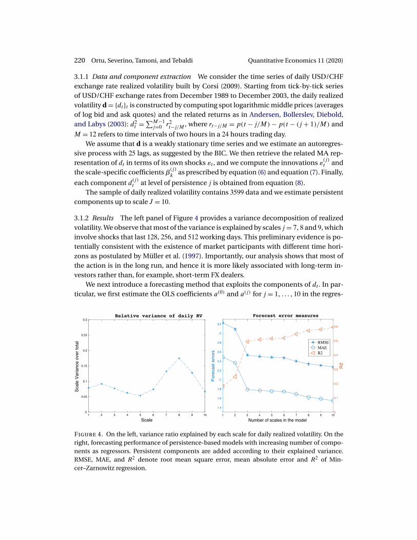
3.1.2 Results The left panel of Figure 4 provides a variance decomposition of realizedvolatility. We observe that most of the variance is explained by scales j = 7�8 and 9, whichinvolve shocks that last 128, 256, and 512 working days. This preliminary evidence is po-tentially consistent with the existence of market participants with different time hori-zons as postulated by Müller et al. (1997). Importantly, our analysis shows that most ofthe action is in the long run, and hence it is more likely associated with long-term in-vestors rather than, for example, short-term FX dealers.

We next introduce a forecasting method that exploits the components of dt . In par-ticular, we first estimate the OLS coefficients a(0) and a(j) for j = 1� � � � �10 in the regres-

Figure 4. On the left, variance ratio explained by each scale for daily realized volatility. On theright, forecasting performance of persistence-based models with increasing number of compo-nents as regressors. Persistent components are added according to their explained variance.RMSE, MAE, and R2 denote root mean square error, mean absolute error and R2 of Min-cer–Zarnowitz regression.

Quantitative Economics 11 (2020) A persistence-based Wold-type decomposition 221

sion

dt = a(0) +J∑

j=1

a(j)d(j)t + ξt� (18)

Then we consider equation (18) at time t + 1, and we apply the conditional expectationat t to obtain the one-step ahead forecast

Et[dt+1] = a(0) +J∑

j=1

a(j)Et[d(j)t+1

]� (19)

To estimate the conditional expectations Et[d(j)t+1] at scales j, we use the forecasting for-mulas that we provide in the Online Supplemental Material A.2. By employing the esti-mates of a(0) and a(j) from equation (18), we obtain a one-day ahead forecast for dt+1based on the components of realized volatility.

Rather than considering all the components at once, we study the performance ofmodels with increased complexity as captured by the number of regressors. In particu-lar, we add one component at a time based on the explained variance reported in theleftmost panel of Figure 4. Hence, we start with a model that includes only the compo-nent j = 8, then we move to a model with two components j = 7�8, and so on. Interest-ingly, the addition of a new component leaves (largely) unaffected the coefficients onthe components included by the previous model. This is so because the Wold compo-nents are uncorrelated by construction. Indeed, one could even impose the restrictiona(j) = 1 with j ∈N as suggested by the extended Wold decomposition.

The right panel of Figure 4 shows the relation between in-sample forecasting perfor-mance and the number of persistent components added according to their explainedvariance. After including the three scales j = 7�8�9, we do not see a meaningful improve-ment in forecasting ability. Hence, our preferred model is given by

dt = a(0) + a(7)d(7)t + a(8)d(8)t + a(9)d(9)t + ξt� (20)

which delivers the forecast

Et[dt+1] = a(0) + a(7)Et[d(7)t+1

] + a(8)Et[d(8)t+1

] + a(9)Et[d(9)t+1

]� (21)

In other words, we are making predictions of daily volatility dt from its long cycles withpersistence of about 128, 256, and 512 days.

Table 1 quantifies the performance of our persistence-based forecasting with threecomponents and compares it with the Heterogeneous Autoregressive model (HAR) ofCorsi (2009). We follow Corsi (2009) and report results for out-of-sample forecasts ofthe realized volatility in which the models are reestimated daily on a moving window of2600 observations.2 The forecasting performances are compared over two different time

2Large moving windows allow for a proper estimation of persistent components at high scales. By using2600 observations, we can build time series of 528 realizations for each component from scale 1 to 9. Inparticular, we want to have at least four coefficients β

(j)k for j = 9. Hence, 2048 observations are required at

any t. Considering 528 realizations of g(9)t , we get 2575 observations. Additional 25 lags are needed in thepreliminary AR estimate of realized volatility.

222 Ortu, Severino, Tamoni, and Tebaldi Quantitative Economics 11 (2020)

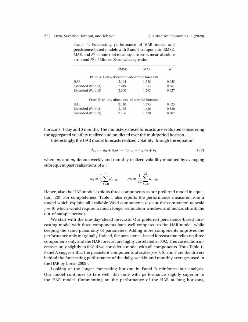
Table 1. Forecasting performance of HAR model andpersistence-based models with 3 and 9 components. RMSE,MAE, and R2 denote root mean square error, mean absoluteerror and R2 of Mincer–Zarnowitz regression.

RMSE MAE R2

Panel A: 1-day-ahead out-of-sample forecastsHAR 2�144 1�548 0�658Extended Wold (3) 2�449 1�873 0�561Extended Wold (9) 2�300 1�705 0�627

Panel B: 66-day-ahead out-of-sample forecastsHAR 2�110 1�693 0�523Extended Wold (3) 2�125 1�646 0�530Extended Wold (9) 2�106 1�620 0�602

horizons: 1 day and 3 months. The multistep-ahead forecasts are evaluated consideringthe aggregated volatility realized and predicted over the multiperiod horizon.

Interestingly, the HAR model forecasts realized volatility through the equation

dt+1 = a0 + addt + awwt + ammt + νt� (22)

where wt and mt denote weekly and monthly realized volatility obtained by averagingsubsequent past realizations of dt :

wt = 15

4∑h=0

dt−h� mt = 122

21∑h=0

dt−h�

Hence, also the HAR model exploits three components as our preferred model in equa-tion (20). For completeness, Table 1 also reports the performance measures from amodel which exploits all available Wold components (except the component at scalej = 10 which would require a much longer estimation window, and hence, shrink theout-of-sample period).

We start with the one-day-ahead forecasts. Our preferred persistence-based fore-casting model with three components fares well compared to the HAR model, whilekeeping the same parsimony of parameters. Adding more components improves theperformance only marginally. Indeed, the persistence-based forecast that relies on threecomponents only and the HAR forecast are highly correlated at 0�92. This correlation in-creases only slightly to 0�96 if we consider a model with all components. Thus Table 1-Panel A suggests that the persistent components at scales j = 7�8, and 9 are the driversbehind the forecasting performance of the daily, weekly, and monthly averages used inthe HAR by Corsi (2009).

Looking at the longer forecasting horizon in Panel B reinforces our analysis.Our model continues to fare well, this time with performance slightly superior tothe HAR model. Commenting on the performance of the HAR at long horizons,

Quantitative Economics 11 (2020) A persistence-based Wold-type decomposition 223

Corsi (2009, p. 192) states: “What is surprising is the ability of the HAR-RV model toattain these results with only a few parameters.” At the light of our analysis, it is clearthat the ability of the model to forecast well at short- and long-horizons is dictated bythe use of components that converge slowly to their unconditional mean relative to theforecasting horizon.

Overall our analysis supports the fact that the forecasting ability of the HAR modeltruly depends on high scales.

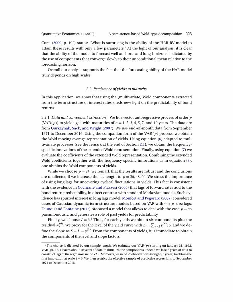
3.2 Persistence of yields to maturity

In this application, we show that using the (multivariate) Wold components extractedfrom the term structure of interest rates sheds new light on the predictability of bondreturns.

3.2.1 Data and component extraction We fit a vector autoregressive process of order p(VAR(p)) to yields y(n)t with maturities of n = 1�2�3�4�5�7, and 10 years. The data arefrom Gürkaynak, Sack, and Wright (2007). We use end-of-month data from September1971 to December 2016. Using the companion form of the VAR(p) process, we obtainthe Wold moving average representation of yields. Using equation (6) adapted to mul-tivariate processes (see the remark at the end of Section 2.1), we obtain the frequency-specific innovations of the extended Wold representation. Finally, using equation (7) weevaluate the coefficients of the extended Wold representation. Combining the extendedWold coefficients together with the frequency-specific innovations as in equation (8),one obtains the Wold components of yields.

While we choose p = 24, we remark that the results are robust and the conclusionsare unaffected if we increase the lag length to p = 36�48�60. We stress the importanceof using long lags for uncovering cyclical fluctuations in yields. This fact is consistentwith the evidence in Cochrane and Piazzesi (2005) that lags of forward rates add to thebond return predictability, in direct contrast with standard Markovian models. Such ev-idence has spurred interest in long lags model: Monfort and Pegoraro (2007) consideredcases of Gaussian dynamic term structure models based on VAR with 0 < p < ∞ lags;Feunou and Fontaine (2017) proposed a model that allows to deal with the case p = ∞parsimoniously, and generates a role of past yields for predictability.

Finally, we choose J = 6.3 Thus, for each yields we obtain six components plus theresidual π(6)

t . We proxy for the level of the yield curve with L = ∑n≥2 y

(n)t /6, and we de-

fine the slope as S = L − y(1)t . From the components of yields, it is immediate to obtainthe components of the level and slope factors.

3The choice is dictated by our sample length. We estimate our VAR(p) starting on January 31, 1962,VAR(p). This leaves about 10 years of data to initialize the components. Indeed we lose 2 years of data toconstruct lags of the regressors in the VAR. Moreover, we need 26 observations (roughly 5 years) to obtain thefirst innovation at scale j = 6. We then restrict the effective sample of predictive regressions to September1971 to December 2016.

224 Ortu, Severino, Tamoni, and Tebaldi Quantitative Economics 11 (2020)

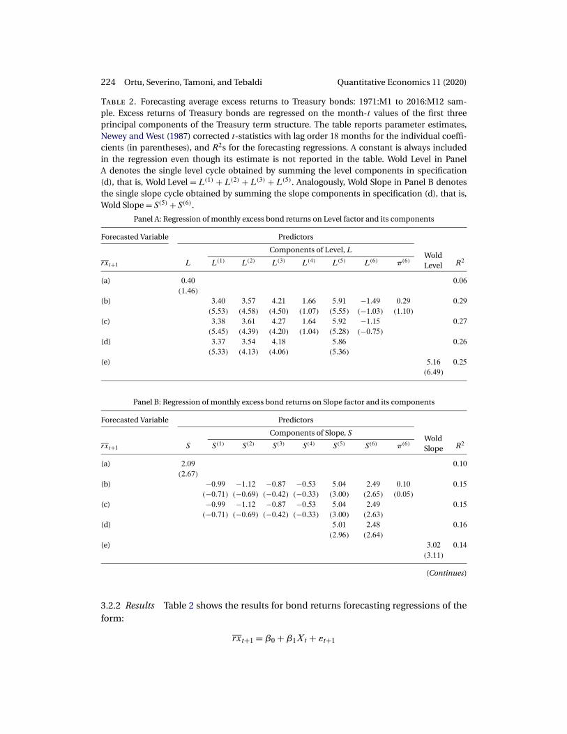
Table 2. Forecasting average excess returns to Treasury bonds: 1971:M1 to 2016:M12 sam-ple. Excess returns of Treasury bonds are regressed on the month-t values of the first threeprincipal components of the Treasury term structure. The table reports parameter estimates,Newey and West (1987) corrected t-statistics with lag order 18 months for the individual coeffi-cients (in parentheses), and R2s for the forecasting regressions. A constant is always includedin the regression even though its estimate is not reported in the table. Wold Level in PanelA denotes the single level cycle obtained by summing the level components in specification(d), that is, Wold Level = L(1) + L(2) + L(3) + L(5). Analogously, Wold Slope in Panel B denotesthe single slope cycle obtained by summing the slope components in specification (d), that is,Wold Slope = S(5) + S(6).

Panel A: Regression of monthly excess bond returns on Level factor and its components

Forecasted Variable Predictors

Components of Level, L

rxt+1 L L(1) L(2) L(3) L(4) L(5) L(6) π(6)WoldLevel R2

(a) 0�40 0�06(1�46)

(b) 3�40 3�57 4�21 1�66 5�91 −1�49 0�29 0�29(5�53) (4�58) (4�50) (1�07) (5�55) (−1�03) (1�10)

(c) 3�38 3�61 4�27 1�64 5�92 −1�15 0�27(5�45) (4�39) (4�20) (1�04) (5�28) (−0�75)

(d) 3�37 3�54 4�18 5�86 0�26(5�33) (4�13) (4�06) (5�36)

(e) 5�16 0�25(6�49)

Panel B: Regression of monthly excess bond returns on Slope factor and its components

Forecasted Variable Predictors

Components of Slope, S

rxt+1 S S(1) S(2) S(3) S(4) S(5) S(6) π(6)WoldSlope R2

(a) 2�09 0�10(2�67)

(b) −0�99 −1�12 −0�87 −0�53 5�04 2�49 0�10 0�15(−0�71) (−0�69) (−0�42) (−0�33) (3�00) (2�65) (0�05)

(c) −0�99 −1�12 −0�87 −0�53 5�04 2�49 0�15(−0�71) (−0�69) (−0�42) (−0�33) (3�00) (2�63)

(d) 5�01 2�48 0�16(2�96) (2�64)

(e) 3�02 0�14(3�11)

(Continues)

3.2.2 Results Table 2 shows the results for bond returns forecasting regressions of theform:

rxt+1 = β0 +β1Xt + εt+1

Quantitative Economics 11 (2020) A persistence-based Wold-type decomposition 225

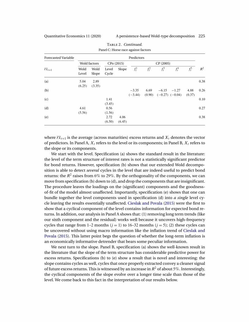
Table 2. Continued.Panel C: Horse race against factors

Forecasted Variable Predictors

Wold factors CPo (2015) CP (2005)

rxt+1 WoldLevel

WoldSlope

LevelCycle

Slope f 1t f 2

t f 3t f 4

t f 5t R2

(a) 5�04 2�89 0�38(6�25) (3�35)

(b) −3�35 6�69 −6�15 −1�27 4�88 0�26(−3�44) (0�90) (−0�27) (−0�04) (0�37)

(c) 1�41 0�10(3�45)

(d) 4�61 0�56 0�27(5�56) (1�56)

(e) 2�72 4�06 0�38(6�50) (6�45)

where rxt+1 is the average (across maturities) excess returns and Xt denotes the vectorof predictors. In Panel A, Xt refers to the level or its components; in Panel B, Xt refers tothe slope or its components.

We start with the level. Specification (a) shows the standard result in the literature:the level of the term structure of interest rates is not a statistically significant predictorfor bond returns. However, specification (b) shows that our extended Wold decompo-sition is able to detect several cycles in the level that are indeed useful to predict bondreturns: the R2 raises from 6% to 29%. By the orthogonality of the components, we canmove from specification (b) down to (d), and drop the components that are insignificant.The procedure leaves the loadings on the (significant) components and the goodness-of-fit of the model almost unaffected. Importantly, specification (e) shows that one canbundle together the level components used in specification (d) into a single level cy-cle leaving the results essentially unaffected. Cieslak and Povala (2015) were the first toshow that a cyclical component of the level contains information for expected bond re-turns. In addition, our analysis in Panel A shows that: (1) removing long term trends (likeour sixth component and the residual) works well because it uncovers high-frequencycycles that range from 1–2 months (j = 1) to 16–32 months (j = 5); (2) these cycles canbe uncovered without using macro information like the inflation trend of Cieslak andPovala (2015). This latter point begs the question of whether the long-term inflation isan economically informative detrender that bears some peculiar information.

We next turn to the slope. Panel B, specification (a) shows the well-known result inthe literature that the slope of the term structure has considerable predictive power forexcess returns. Specifications (b) to (e) show a result that is novel and interesting: theslope contains cycles as well, cycles that once properly extracted convey a cleaner signalof future excess returns. This is witnessed by an increase in R2 of about 5%. Interestingly,the cyclical components of the slope evolve over a longer time scale than those of thelevel. We come back to this fact in the interpretation of our results below.

226 Ortu, Severino, Tamoni, and Tebaldi Quantitative Economics 11 (2020)

Panel C compares our level and slope factors extracted using the extended Wold de-composition with other factors employed in the literature. The first row is our bench-mark model where we use the level and slope factors from specification (e) in Panel Aand B together to predict bond returns. Our factors are (close to) orthogonal as testi-fied by the fact that the R2 of the multiple regression is close to the sum of the R2 fromsimple regressions. Specification (b) is akin to the Cochrane and Piazzesi (2005) model,and it shows that a linear combination of forward rates has predictive ability above andbeyond the slope (cf. Panel B, specification (a)). Yet, the goodness-of-fit of the Cochraneand Piazzesi (2005) is lower than our benchmark specification by about 12%. Specifica-tion (c) is akin to the Cieslak and Povala (2015) level factor: in particular, we remove fromthe level of the yield curve a secular inflation trend. Consistent with Cieslak and Povala(2015), the level cycle so constructed has forecasting ability for bond returns. However,specification (d) shows that the level cycle extracted using our extended Wold decom-position drives away a level cycle obtained using an inflation trend.

Specification (e) is akin to the full specification by Cieslak and Povala (2015). Rebon-ato and Hatano (2018) showed that the Cieslak and Povala (2015) factor can be rewrittenas a combination of the slope and the detrended level used in specification (c). Two re-marks are in order. First, the Cieslak and Povala (2015) specification attains the same fitas our benchmark model with components of the level and slope extracted from the ex-tended Wold. Both specifications are based on a high-frequency component related tothe level and a low-frequency component related to the slope (recall that our level fac-tor is composed of components j = 1�2�3�5 as per specification (d) in Panel A, whereasour slope factor is composed of components j = 5�6 as per specification (d) in Panel B).Despite these similarities, the two models call for potentially different economic expla-nations. This leads to our second remark. Our benchmark specification (a) provides avery simple attribution of the predictability: 25% comes from the high-frequency cyclein the level (cf. specification (e) in Panel A), and 14% comes from the low-frequency cy-cle in the slope (cf. specification (e) in Panel B), for a total of about 38% (cf. specification(a) in Panel C). One can then try to link these two frequencies to economic factors evolv-ing over different time scales. For instance, Rebonato and Hatano (2018) linked the slopeto business cycle fluctuations induced by time-varying risk aversion, and the high fre-quency cycle in the level to temporary deterioration in market liquidity by arbitrageurs.On the other hand, specification (e) shows that one needs to consider also a third factor.This is clearly seen by observing that the sum of the R2 statistics from the two separatereturn predictive factors (cf. specification (a) in Panel B and specification (c) in PanelC) falls short of adding up to the full explanatory power of the bivariate regression (cf.specification (e) in Panel C). Together, the level cycle and the slope of the yield curveenhance the explanatory power because they are strongly negative correlated at −47%.Overall, specification (e) requires: (1) an economic story for the high frequency compo-nent in the level; (2) an economic story for the low frequency component in the slope;and (3) a third factor to explain that the relative values of the slope and detrended levelis important.

Comparing specification (a) to specification (e) we can sum up our main findingsas follows: (1) it is possible to recover the same goodness-of-fit without using long term

Quantitative Economics 11 (2020) A persistence-based Wold-type decomposition 227

inflation trends: this fact raises concern whether the long-term inflation detrending isreally special; (2) despite the same statistical fit, the two specifications call for a differentnumber of factors: our approach relies on the orthogonality of the components and doesnot need to explain interaction terms in the attribution of predictability.

4. Conclusions

We provide an orthogonal decomposition of xt into uncorrelated components g(j)t that

are associated with different layers of persistence. This decomposition, which we dubExtended Wold Decomposition, results from the application of the abstract Wold theo-rem on the Hilbert space Ht (ε), spanned by the classical Wold innovations of x, wherethe scaling operator R is isometric. We also show how to construct a stationary time se-ries starting from the law of motion of the components g

(j)t defined over different time

scales.From a technical perspective, our Wold-type decomposition of weakly stationary

stochastic processes is the outcome of a multiresolution analysis of an abstract Hilbertspace and it is connected to the work by Baggett, Larsen, Packer, Raeburn, and Ram-say (2010), where the authors study the wavelet decompositions of Hilbert spaces. Theirconstruction and our approach rely on the isometry associated with the operator: this iskey to permit the use of the abstract Wold theorem (see Nagy et al. (2010)).

From an empirical perspective, we see our extended Wold decomposition as a usefultool for the analysis of macroeconomic and financial time series that are commonly af-fected by shocks with different frequencies. Using two applications, we have shown thatthe ability of our extended Wold decomposition to separate and zoom-in the differentfluctuations which may coexist in the original time series has important consequencesfor forecasting, as well as the economic interpretation of the results. In addition, Di Vir-gilio, Ortu, Severino, and Tebaldi (2019) provided an application of our theory to optimalasset allocation when security returns are subject to shocks with heterogeneous persis-tence.

Our extended Wold decomposition is based on the estimated moving average co-efficients. Thus, uncertainty around the Wold coefficients affect inference on the Woldcomponents. In this paper, we fit a VAR of length p on the underlying process to recoverits infinite moving average representation. Similar to what is done in the (Structural)VAR literature to compute confidence intervals for impulse response functions, one canquantify the uncertainty around the Wold components by, for example, bootstrappingthe data using the estimated VAR parameters and the fitted residuals. Alternatively, onecould conduct inference directly on the moving average representation of the data (with-out estimation and inversion of the VAR) along the line of Barnichon and Matthes (2018)and Plagborg-Moller (2019). We view this as an interesting avenue for future research.

References

Addison, P. S. (2002), The Illustrated Wavelet Transform Handbook: Introductory Theoryand Applications in Science, Engineering, Medicine and Finance. CRC Press. [209]

228 Ortu, Severino, Tamoni, and Tebaldi Quantitative Economics 11 (2020)

Andersen, T. G. and T. Bollerslev (1997), “Heterogeneous information arrivals and returnvolatility dynamics: Uncovering the long-run in high frequency returns.” The Journal ofFinance, 52 (3), 975–1005. [206, 219]

Andersen, T. G., T. Bollerslev, F. X. Diebold, and P. Labys (2003), “Modeling and forecast-ing realized volatility.” Econometrica, 71 (2), 579–625. [220]

Baggett, L. W., N. S. Larsen, J. A. Packer, I. Raeburn, and A. Ramsay (2010), “Direct limits,multiresolution analyses, and wavelets.” Journal of Functional Analysis, 258 (8), 2714–2738. [227]

Bandi, F., A. W. Lo, S. Chaudhuri, and A. Tamoni (2019), “Spectral factor models.” Re-search Paper 18-17, John Hopkins Carey Business School. [205]

Bandi, F., B. Perron, A. Tamoni, and C. Tebaldi (2019), “The scale of predictability.” Jour-nal of Econometrics, 208 (1), 120–140. [205]

Barnichon, R. and C. Matthes (2018), “Functional approximation of impulse responses.”Journal of Monetary Economics, 99 (C), 41–55. [227]

Calvet, L. E. and A. J. Fisher (2007), “Multifrequency news and stock returns.” Journal ofFinancial Economics, 86 (1), 178–212. [206]

Cerreia-Vioglio, S., F. Ortu, F. Severino, and C. Tebaldi (2017), “Multivariate Wold decom-positions.” IGIER Working Paper n. 606. [212]

Cieslak, A. and P. Povala (2015), “Expected returns in treasury bonds.” The Review of Fi-nancial Studies, 28 (10), 2859–2901. [205, 225, 226]

Cochrane, J. H. and M. Piazzesi (2005), “Bond risk premia.” American Economic Review,95 (1), 138–160. [223, 226]

Corsi, F. (2009), “A simple approximate long-memory model of realized volatility.” Jour-nal of Financial Econometrics, 7 (2), 174–196. [205, 206, 221, 222, 223]

Di Virgilio, D., F. Ortu, F. Severino, and C. Tebaldi (2019), “Optimal asset allocation withheterogeneous persistent shocks and myopic and intertemporal hedging demand.” InBehavioral Finance: The Coming of Age, 57–108, World Scientific. [227]

Engle, R. F. and G. Lee (1999), A Long-Run and Short-Run Component Model of Stock Re-turn Volatility. Cointegration, Causality, and Forecasting. Oxford University Press. [206]

Engle, R. F. and J. G. Rangel (2008), “The spline-GARCH model for low-frequency volatil-ity and its global macroeconomic causes.” Review of Financial Studies, 21 (3), 1187–1222.[206]

Feunou, B. and J.-S. Fontaine (2017), “Bond risk premia and Gaussian term structuremodels.” Management Science, 64 (3), 1413–1439. [223]

Ghysels, E., P. Santa-Clara, and R. Valkanov (2004), “The MIDAS touch: Mixed data sam-pling regression models.” CIRANO Working Papers 2004s-20, CIRANO. [206]

Quantitative Economics 11 (2020) A persistence-based Wold-type decomposition 229

Ghysels, E., P. Santa-Clara, and R. Valkanov (2006), “Predicting volatility: Getting themost out of return data sampled at different frequencies.” Journal of Econometrics, 131(1–2), 59–95. [206]

Granger, C. W. J. (1980), “Long memory relationships and the aggregation of dynamicmodels.” Journal of Econometrics, 14 (2), 227–238. [204]

Gürkaynak, R. S., B. Sack, and J. H. Wright (2007), “The US Treasury yield curve: 1961 tothe present.” Journal of Monetary Economics, 54 (8), 2291–2304. [223]

Monfort, A. and F. Pegoraro (2007), “Switching VARMA term structure models-extendedversion.” Working Papers 191, Banque de France. [223]

Müller, U. A., M. Dacorogna, R. D. Dave, O. V. Pictet, R. Olsen, and J. Ward (1993), “Frac-tals and intrinsic time—a challenge to econometricians.” Working Papers 1993-08-16,Olsen and Associates. [205]

Müller, U. A., M. M. Dacorogna, R. D. Davé, R. B. Olsen, O. V. Pictet, and J. E. vonWeizsäcker (1997), “Volatilities of different time resolutions—analyzing the dynamicsof market components.” Journal of Empirical Finance, 4 (2), 213–239. [219, 220]

Müller, U. K. and M. W. Watson (2008), “Testing models of low-frequency variability.”Econometrica, 76 (5), 979–1016. [206]

Müller, U. K. and M. W. Watson (2017), “Low-frequency econometrics.” In Advances inEconomics and Econometrics: Volume 2: Eleventh World Congress, Vol. 2, 53. CambridgeUniversity Press. [206]

Nagy, B. S., C. Foias, H. Bercovici, and L. Kérchy (2010), Harmonic Analysis of Operatorson Hilbert Space. Springer. [210, 227]

Newey, W. K. and K. D. West (1987), “Hypothesis testing with efficient method of mo-ments estimation.” International Economic Review, 777–787. [224]

Ortu, F., Severino, F., Tamoni, A., and Tebaldi, C. (2020), “Supplement to ‘A persistence-based Wold-type decomposition for stationary time series’.” Quantitative EconomicsSupplemental Material, 11, https://doi.org/10.3982/QE994. [206]

Ortu, F., A. Tamoni, and C. Tebaldi (2013), “Long-run risk and the persistence of con-sumption shocks.” Review of Financial Studies, 26 (11), 2876–2915. [204, 205, 206, 217]

Plagborg-Moller, M. (2019), “Bayesian inference on structural impulse response func-tions.” Quantitative Economics, 10 (1), 145–184. [227]

Rebonato, R. and T. Hatano (2018), “The economic origin of treasury excess returns: Acycles and trend explanation.” [226]

Robinson, P. M. (1978), “Statistical inference for a random coefficient autoregressivemodel.” Scandinavian Journal of Statistics, 5 (3), 163–168. [204]

Severino, F. (2016), “Isometric operators on Hilbert spaces and Wold decomposition ofstationary time series.” Decisions in Economics and Finance, 39 (2), 203–234. [211]

230 Ortu, Severino, Tamoni, and Tebaldi Quantitative Economics 11 (2020)

Wold, H. (1938), A Study in the Analysis of Stationary Time Series. Almqvist & WiksellsBoktryckeri. [209]

Co-editor Frank Schorfheide handled this manuscript.

Manuscript received 3 October, 2017; final version accepted 4 August, 2019; available online 14August, 2019.