A Performance Evaluation Methodology to Find the Best Parallel ...

UNIVERSIDADE FEDERAL DO RIO GRANDE DO SULINSTITUTO DE INFORMÁTICA

PROGRAMA DE PÓS-GRADUAÇÃO EM COMPUTAÇÃO

LUÍS FELIPE GARLET MILLANI MILLANI

A Performance Evaluation Methodologyto Find the Best Parallel Regions to

Reduce Energy Consumption

Thesis presented in partial fulfillmentof the requirements for the degree ofMaster of Computer Science

Advisor: Prof. Dr. Nicolas MaillardCoadvisor: Prof. Dr. Lucas Mello Schnorr

Porto AlegreNovember 2015

CIP — CATALOGING-IN-PUBLICATION

Millani, Luís Felipe Garlet Millani

A Performance Evaluation Methodology to Find theBest Parallel Regions to Reduce Energy Consumption/ Luís Felipe Garlet Millani Millani. – Porto Alegre:PPGC da UFRGS, 2015.

55 f.: il.

Thesis (Master) – Universidade Federal do Rio Grandedo Sul. Programa de Pós-Graduação em Computação,Porto Alegre, BR–RS, 2015. Advisor: Prof. Dr. Nicolas Mail-lard; Coadvisor: Prof. Dr. Lucas Mello Schnorr.

1. Methodology. 2. Energy. 3. HPC. 4. DVFS. 5. Mul-ticore. 6. Performance. 7. OpenMP. I. Nicolas Maillard,Prof. Dr.. II. Lucas Mello Schnorr, Prof. Dr.. III. Título.

UNIVERSIDADE FEDERAL DO RIO GRANDE DO SULReitor: Prof. Carlos Alexandre NettoVice-Reitor: Prof. Rui Vicente OppermannPró-Reitor de Pós-Graduação: Prof. Vladimir Pinheiro do NascimentoDiretor do Instituto de Informática: Prof. Luis da Cunha LambCoordenador do PPGC: Prof. Luigi CarroBibliotecária-chefe do Instituto de Informática: Beatriz Regina Bastos Haro

ACKNOWLEDGEMENTS

• Agradeço aos meus pais, Francisco e Eleonor, e a meu irmão Marcelo.

• Agradeço ao meu orientador, Nicolas Maillard.

• Agradeço ao meu co-orientador, Lucas Schnorr, principalmente pelas dicas

de escrita.

• Agradeço ao Arnaud Legrand pelo auxílio no projeto de experimentos.

• Agradeço ao pessoal do laboratório 205.

• Agradeço ao CNPq pelo auxílio financeiro.

ABSTRACT

Due to energy limitations imposed to supercomputers, parallel applications de-

veloped for High Performance Computers (HPC) are currently being investigated

with energy efficiency metrics. The idea is to reduce the energy footprint of these

applications. While some energy reduction strategies consider the application as

a whole, certain strategies adjust the core frequency only for certain regions of the

parallel code. Load balancing or blocking communication phases could be used

as opportunities for energy reduction, for instance. The efficiency analysis of such

strategies is usually carried out with traditional methodologies derived from the

performance analysis domain. It is clear that a finer grain methodology, where

the energy reduction is evaluated per each code region and frequency configura-

tion, could potentially lead to a better understanding of how energy consumption

can be reduced for a particular algorithm implementation. To get this, the main

challenges are: (a) the detection of such, possibly parallel, code regions and the

large number of them; (b) which frequency should be adopted for that region (to

reduce energy consumption without too much penalty for the runtime); and (c)

the cost to dynamically adjust core frequency. The work described in this dis-

sertation presents a performance analysis methodology to find the best parallel

region candidates to reduce energy consumption. The proposal is three folded:

(a) a clever design of experiments based on screening, especially important when

a large number of parallel regions is detected in the applications; (b) a traditional

energy and performance evaluation on the regions that were considered as good

candidates for energy reduction; and (c) a Pareto-based analysis showing how

hard is to obtain energy gains in optimized codes. In (c), we also show other

trade-offs between performance loss and energy gains that might be of interest of

the application developer. Our approach is validated against three HPC applica-

tion codes: Graph500; Breadth-First Search, and Delaunay Refinement.

Keywords: Methodology. energy. HPC. DVFS. multicore. performance. OpenMP.

Uma Metodologia de Avaliação de Desempenho para Identificar as Melhores

Regiões Paralelas para Reduzir o Consumo de Energia.

RESUMO

Devido as limitações de consumo energético impostas a supercomputadores, mé-

tricas de eficiência energética estão sendo usadas para analisar aplicações para-

lelas desenvolvidas para computadores de alto desempenho. O objetivo é a re-

dução do custo energético dessas aplicações. Algumas estratégias de redução de

consumo energética consideram a aplicação como um todo, outras reduzem ajus-

tam a frequência dos núcleos apenas em certas regiões do código paralelo. Fases

de balanceamento de carga ou de comunicação bloqueante podem ser oportunas

para redução do consumo energético. A análise de eficiência dessas estratégias

é geralmente realizada com metodologias tradicionais derivadas do domínio de

análise de desempenho. Uma metodologia de grão mais fino, onde a redução

de energia é avaliada para cada região de código e frequência pode lever a um

melhor entendimento de como o consumo energético pode ser minimizado para

uma determinada implementação. Para tal, os principais desafios são: (a) a detec-

ção de um número possivelmente grande de regiões paralelas; (b) qual frequência

deve ser adotada para cada região de forma a limitar o impacto no tempo de exe-

cução; e (c) o custo do ajuste dinâmico da frequência dos núcleos. O trabalho

descrito nesta dissertação apresenta uma metodologia de análise de desempenho

para encontrar, dentre as regiões paralelas, os melhores candidatos a redução do

consumo energético. Esta proposta consiste de: (a) um design inteligente de ex-

perimentos baseado em Plackett-Burman, especialmente importante quando um

grande número de regiões paralelas é detectado na aplicação; (b) análise tradicio-

nal de energia e desempenho sobre as regiões consideradas candidatas a redução

do consumo energético; e (c) análise baseada em eficiência de Pareto mostrando

a dificuldade em otimizar o consumo energético. Em (c) também são mostrados

os diferentes pontos de equilíbrio entre desempenho e eficiência energética que

podem ser interessantes ao desenvolvedor. Nossa abordagem é validada por três

aplicações: Graph500, busca em largura, e refinamento de Delaunay.

Palavras-chave: Metodologia, Energia, Alto Desempenho, DVFS, Paralelismo,

OpenMP.

LIST OF ABBREVIATIONS AND ACRONYMS

ANOVA ANalysis Of VAriance

BFS Breadth-First Search

DVFS Dynamic Voltage and Frequency Scaling

EDP Energy-Delay Product

MEPlot Main Effects Plot

MSR Model-Specific Register

NUMA Non-Uniform Memory Access

NVML Nvidia Management Library

PBBS Problem Based Benchmark Suite

RAPL Running Average Power Limit

LIST OF FIGURES

Figure 2.1 Execution time and energy consumption as a function of differ-ent frequency configurations used to execute a Matrix Product appli-cation......................................................................................................................16

Figure 3.1 Comparison between the traditional and the proposed method-ologies. ...................................................................................................................19

Figure 3.2 Example of experimental designs for three factors...............................20Figure 3.3 Two objective functions with no single point minimizing both. ........22

Figure 4.1 Example of the types of graphs used as input for the PBBS bench-mark. ......................................................................................................................28

Figure 4.2 MEPlot for energy consumption of the Graph500 benchmark. ..........30Figure 4.3 MEPlot for time of the Graph500 benchmark........................................31Figure 4.4 MEPlot for the energy-delay product of the Graph500 benchmark...32Figure 4.5 Average energy consumption, runtime and energy-delay prod-

uct as a function of different strategies of frequency configurations forthe Graph500 benchmark....................................................................................35

Figure 4.6 Energy-runtime Pareto front of the Graph500 benchmark..................36Figure 4.7 Power-runtime Pareto front of the Graph500 benchmark. ..................37Figure 4.8 MEPlot for energy consumption the Breadth-First Search bench-

mark. ......................................................................................................................38Figure 4.9 MEPlot for time of the Breadth-First Search benchmark. ....................39Figure 4.10 MEPlot for the energy-delay product of the Breadth-First Search

benchmark.............................................................................................................40Figure 4.11 Average energy consumption, runtime and energy-delay prod-

uct as a function of different strategies of frequency configurations forthe Breadth-First Search benchmark. ................................................................41

Figure 4.12 Pareto front for runtime and energy of the Breadth-First Searchbenchmark.............................................................................................................43

Figure 4.13 Pareto front for runtime and power of the Breadth-First Searchbenchmark.............................................................................................................44

Figure 4.14 MEPlot for the energy consumption of the Delaunay benchmark...45Figure 4.15 MEPlot for time of the Delaunay benchmark......................................45Figure 4.16 MEPlot for the Energy-Delay product of the Delaunay benchmark.46Figure 4.17 Average energy consumption, runtime and energy-delay prod-

uct as a function of different strategies of frequency configurations forthe Delaunay Refine benchmark........................................................................49

Figure 4.18 Pareto front for runtime and energy of the Delaunay Refinebenchmark.............................................................................................................50

Figure 4.19 Pareto front for runtime and power of the Delaunay Refine bench-mark. ......................................................................................................................51

LIST OF TABLES

Table 4.1 Configuration of the experimental platform............................................25Table 4.2 ANOVA of energy consumption of the Graph500 benchmark. ............31Table 4.3 ANOVA of runtime of the Graph500 benchmark. ..................................32Table 4.4 ANOVA of energy-delay product of the Graph500 benchmark. ..........33Table 4.5 Results of the Graph500 benchmark. ........................................................34Table 4.6 ANOVA of energy consumption of the Breadth-First Search bench-

mark. ......................................................................................................................38Table 4.7 ANOVA of runtime of the Breadth-First Search benchmark.................39Table 4.8 ANOVA of energy-delay product of the Breadth-First Search bench-

mark. ......................................................................................................................40Table 4.9 Results of the Breadth-First Search benchmark.......................................41Table 4.10 ANOVA of energy reduction effect of the Delaunay benchmark. ......45Table 4.11 ANOVA of runtime of the Delaunay benchmark. ................................46Table 4.12 ANOVA of energy-delay product of the Delaunay benchmark. ........47Table 4.13 Results of the Delaunay Refine benchmark. ..........................................48

CONTENTS

1 INTRODUCTION.....................................................................................................111.1 Proposal and Objective........................................................................................121.2 Text structure..........................................................................................................132 RELATED WORK AND BASIC CONCEPTS .....................................................142.1 Estimating Energy Consumption.......................................................................142.2 Energy-Delay Product ..........................................................................................162.3 Main Effects Plot ...................................................................................................173 A NEW PERFORMANCE ANALYSIS METHODOLOGY...............................183.1 Screening Multiple Code Regions.....................................................................183.2 Traditional Performance/Energy Analysis .......................................................213.3 Full Factorial ..........................................................................................................213.4 Pareto Analysis for Different Trade-offs ..........................................................224 EXPERIMENTAL EVALUATION ..........................................................................244.1 Experimental Platform and Software Description .........................................244.1.1 libenergy...............................................................................................................254.2 Benchmarks Description .....................................................................................264.2.1 The Graph500 Benchmark .................................................................................264.2.2 PBBS Suite: the Breadth-First Search Algorithm............................................274.2.3 PBBS Suite: the Delaunay Refinement Algorithm .........................................284.3 Experimental Results and Analysis...................................................................294.3.1 Analysis of the Graph5000 Benchmark............................................................294.3.2 Analysis of the Breadth-First Search Benchmark ...........................................374.3.3 Analysis of the Delaunay Refinement Benchmark ........................................445 CONCLUSION..........................................................................................................52REFERENCES ...............................................................................................................53

11

1 INTRODUCTION

Performance has historically overshadowed energy efficiency in the HPC

field. Even if in the latest years the situation has changed a little, most publi-

cations still only consider performance in their evaluations, ignoring energy effi-

ciency. This is the case of the Top500 list (MEUER et al., 2014), which ranks the top

supercomputers of the world by their performance when executing the Linpack

benchmark (DONGARRA; LUSZCZEK, 2011a). In the last few years this scenario

began to change and initiatives focusing on energy efficiency, like the Green500

list (SUBRAMANIAM et al., 2014), have gained importance. There are several

factors behind this change. Financially there is certain pressure to reduce energy

consumption due to the direct impact of energy on the running costs of the sys-

tem. Still on the financial side, the heat resulting from the consumed energy has

costs to dissipate and decreases reliability (KIM; BUYYA; KIM, 2007; VASIc et al.,

2009). The costs with energy and heat dissipation are becoming a more signifi-

cant portion of the total costs of HPC systems (GE et al., 2010; SCARAMELLA,

2006). As a large portion of the world’s energy generation comes from pollutant

sources, there is also an environmental reason to reduce energy consumption.

Lastly, the low energy efficiency is quickly becoming a limiting factor in attaining

higher performance (RAJOVIC et al., 2013; FENG; CAMERON, 2007).

The price we pay for low energy efficiency is heightened as exascale com-

puting (GELLER, 2011) comes to our grasp. An exascale computer is expected to

need millions of computational units and many accelerators. The 20 megawatts

(MW) power input is considered an economically feasible limit for a system of

this scale (TORRELLAS, 2009). Although at first this limit may seems large,

it is merely 2.2MW more than the power used by Tianhe-2, the current leader

of Top500 list. Tianhe-2 has an energy efficiency of only 1.9GFLOP per Watt,

whereas a 20MW exascale computer would need 50GFLOPs per Watt. Even the

current leader of Green500, L-CSC, does only 5.3GFLOPs per Watt. Higher en-

ergy efficiency will be mandatory (FENG; CAMERON, 2007) to maintain perfor-

mance improvements for high performance parallel (HPC) applications.

Energy reduction strategies usually operate by adjusting the core frequency

only for a certain region of the parallel application code. The techniques are usu-

ally coupled with algorithms that use some characteristic of the parallel appli-

12

cation to act. For example, there are strategies exploring code regions dedicated

to load balancing to reduce energy consumption (PADOIN et al., 2014), as well

energy reduction strategies based on blocking communication phases of parallel

applications (LIM; FREEH; LOWENTHAL, 2006; ROUNTREE et al., 2009), ac-

tivated when processes are idle. Other coarse grain strategies (GE et al., 2010),

acting in the process or thread level, work by viewing the threads of the appli-

cation as a whole, without paying attention to which part of the code is being

executed to evaluate energy reduction opportunities. On these cases, the code re-

gions are thread-dependent. Independently of which energy reduction strategy is

adopted, the verification of the efficiency of such strategies are usually carried out

with traditional methodologies derived from the performance analysis domain.

It is clear that a finer grain analysis methodology, where the energy reduc-

tion is evaluated per each code region and frequency configuration, could poten-

tially lead to a better understanding of how energy consumption can be reduced

for a particular algorithm implementation. Even if such fine-grain approach does

exist, it is very hard to evaluate the potential benefits of controlling the frequency

in a per-code region fashion. The main challenges include (a) the detection of

such, possibly parallel, code regions and the large number of them; (b) which fre-

quency should be adopted for that region (to reduce energy consumption without

too much penalty for the runtime); and (c) the cost to dynamically adjust core fre-

quency. For all these reasons, we observe the need of a new performance analy-

sis methodology that evaluates the energy consumption of each of the numerous

parallel regions of HPC applications in a separate manner. The result of such new

analysis methodology should be able to provide new and definitive insights on

which core frequency should be adopted to each code region of the parallel appli-

cation. As runtime performance is fundamental in HPC systems, results should

be correlated with performance loss due to frequency reduction.

1.1 Proposal and Objective

The work described in this dissertation presents a performance analysis

evaluation methodology to find the best candidates among the parallel regions

to improve energy consumption. The proposal is three folded: (a) a clever design

of experiments based on screening, especially important when a large number

13

of parallel regions is detected in the applications; (b) a traditional energy and

performance evaluation on the regions that were considered as good candidates

for energy reduction; and (c) a Pareto-based analysis showing how hard is to

obtain energy gains in optimized codes. In (c), we also show other trade-offs

between performance loss and energy gains that might be of interest of the appli-

cation developer. Our approach is validated against three HPC applications im-

plemented with OpenMP: Graph500 (MURPHY et al., 2010); Breadth-First Search

(BFS) (SHUN et al., 2012; BLELLOCH et al., 2012); and Delaunay Refine, which is

part of the same benchmarks suite of BFS.

Supposing that parallel regions can be automatically annotated by a com-

piler, our approach brings the benefit of detecting those regions of code that are

the best candidates for energy reduction by applying frequency scaling on the

cores executing that region. We contribute with a software tool that improves the

energy efficiency of HPC applications without compromising performance nor

requiring unreasonable effort from the developer.

1.2 Text structure

The remainder of this dissertation is structured as follows. Chapter 2 shows

related work – on strategies for energy reduction when executing HPC applica-

tions – and basic concepts, such as methods of estimating the energy used by an

application in a specific system. Chapter 3 presents our proposal for a new perfor-

mance analysis methodology focused on parallel regions of HPC applications. In

this chapter we also discuss implementation details and the method’s advantages

along with its limitations. Chapter 4 shows the experimental results obtained by

applying the new performance analysis methodology previously described. We

evaluate the effectiveness of our approach for three HPC parallel applications. Fi-

nally, Chapter 5 presents our conclusions, highlights the main contributions and

describe future directions.

14

2 RELATED WORK AND BASIC CONCEPTS

This chapter presents the state-of-the-art on energy reduction strategies

already applied for HPC applications. We show that most of current strategies

are coarse grained for the core or process level. We also presents basic concepts

that we consider fundamental to a good understanding of the results shown on

Chapter 4.

2.1 Estimating Energy Consumption

Energy consumption can be measured through a power meter physically

connected to components like CPU, GPU, memory or power supply unit. The

power data gathered by the power meter is usually coarse-grained, with a sam-

pling frequency of 1Hz being usual (DAVIS et al., 2011; LAWSON; SOSONK-

INA; SHEN, 2014). This frequency is sufficient to estimate energy consumption

over long periods of time. However, short spikes are not noticeable (MEISNER;

WENISCH, 2010). Since the power meter is external it does not alter the applica-

tion execution in any meaningful way.

An alternative to the use of external tools is to estimate energy consump-

tion through performance counters available in the hardware. The hardware sup-

port allows finer-grained measure of energy consumption. The finer grain allows

the user to estimate energy consumption of short executions. This enables the es-

timation of the energy consumption of short benchmarks or even of parts of the

application.

The use of the in-hardware performance counters has the downside of re-

quiring code execution to read the counters. This causes a certain overhead, pos-

sibly high if the sampling frequency is high as well. In the case of Intel, the RAPL

counters can result in low overhead since there is an energy counter which ac-

cumulates the power consumption over time, reducing the required sampling

frequency.

In the Intel processors that support it, energy usage can be obtained from

certain Model-Specific Registers (MSR), through the Running Average Power Limit

(RAPL) interface (INTEL, 2013). RAPL makes available the energy and power

used by the memory, the cores or the package as a whole, updated every millisec-

15

ond.

Although this work focuses on the CPU, similar counters are also available

for other components. Motherboards with a Baseboard Management Controller

make energy consumption data available through the Intelligent Platform Man-

agement Interface. The Nvidia Tesla and Quadro GPUs have similar features to

Intel CPUs. Estimates of power consumption of the whole board, including mem-

ory, can be obtained through the Nvidia Management Library (NVML) (NVIDIA,

2012). However, unlike Intel, energy values are not directly available.

Dynamic Voltage and Frequency Scaling

Dynamic Voltage and Frequency Scaling (DVFS) is one technique employed

to reduce the energy footprint of an application. It is proven to be a feasible tech-

nique for this purpose (HSU; FENG, 2005a) and is employed on many scenar-

ios (CHOI; SOMA; PEDRAM, 2005a; HSU; FENG, 2005b; GE et al., 2007), such

as real-time systems, embedded systems and HPC. The technique is based on

the fact that lowering a processor’s frequency reduces its dynamic power usage,

thus reducing instantaneous power use. Despite this, energy consumption can

be higher for lower frequencies than for higher frequencies because the static

leakage stays the same (VOGELEER et al., 2014) and execution time can greatly

increase.

A situation where lower frequencies increase energy consumption is illus-

trated in Figures 2.1a and 2.1b (using boxplots and points representing all mea-

surements). Reducing the frequency from 2.3GHz downward, energy consump-

tion is improved until 1.8GHz. Past that point, energy consumption increases

as the frequency decreases. It should be noted that the effect on energy also de-

pends on the profile of the application, with the execution time of CPU-bound

applications being less affected than that of memory-bound applications due to

the memory bottleneck of the later.

The energy gains achievable through this technique are declining due to

technological advances like higher memory performance and smaller transistor

feature sizes (SUEUR; HEISER, 2010). Higher memory performance reduces the

maximum energy savings obtainable through DVFS since it decreases the amount

of time the processor stays idle waiting for the memory. The smaller transistor

feature size results in a smaller ratio between dynamic power and static leakage.

16

As this ratio decreases, the energy savings decrease and the cost of leakage due

to the greater execution times increases.

DVFS is commonly available on Intel and AMD processors. The frequency

of each core is independent of the frequency of the other cores if each core has

its own clock domain. When clock domains are shared among several cores, they

must run at the same frequency. Virtual cores, for instance, depend on the fre-

quency of their physical counterpart.

Figure 2.1: Execution time and energy consumption as a function of differentfrequency configurations used to execute a Matrix Product application.

1.0

1.2

1.4

1.6

1.2GHz

1.3GHz

1.4GHz

1.5GHz

1.6GHz

1.7GHz

1.8GHz

1.9GHz

2.0GHz

2.1GHz

2.2GHz

2.3GHz

2.301

GHz

Frequency

Tim

e (n

orm

aliz

ed b

y hi

ghes

t fre

quen

cy)

(a) Execution time.

0.96

0.99

1.02

1.2GHz

1.3GHz

1.4GHz

1.5GHz

1.6GHz

1.7GHz

1.8GHz

1.9GHz

2.0GHz

2.1GHz

2.2GHz

2.3GHz

2.301

GHz

Frequency

Ener

gy (n

orm

aliz

ed b

y hi

ghes

t fre

quen

cy)

(b) Energy.

2.2 Energy-Delay Product

Flops per Watt is one of the main metrics to measure energy efficiency (BROOKS

et al., 2000). The Energy-delay Product (HOROWITZ; INDERMAUR; GONZA-

LEZ, 1994) (EDP) is a similar metric, but with a greater emphasis on performance,

making it equivalent toFlops2

Wor

Flops3

W, depending on the weight used. A

greater value for Flops per Watt means greater energy efficiency. But since EDP

uses seconds instead of floating point instructions per second, lower values of

EDP mean greater energy efficiency. In this work, whenever EDP is mentioned

we refer to the following definition:

EDP = Energy · Time = Power · Time2

17

2.3 Main Effects Plot

The main effects plot is used to analyse how each of the factors analysed

(e.g. CPU frequency) affects the response (e.g. energy consumption). The main

effect of each factor is the difference between the mean response for that factor

considering its two possible levels (BOX; HUNTER; HUNTER, 2005). Given y− is

the set of responses for all observations where the level of a factor is −, and y+ is

the set of responses for all observations where the level of that same factor is +,

the main effect of that factor on the response is:

MainEffect = y+ − y−

The main effect can be used with factorial designs. For instance, later

on Figure 3.2b, the results of the four observations would be used to estimate

each of the main effects. This improves the precision given by each observation

when compared to using the one-factor-at-a-time method, which would isolate

all factors and consider them separately. Statistics for situations where more than

two possible values for a given factor are not yet well established. For such rea-

son, we limit our work to the study of extreme frequency configurations.

18

3 A NEW PERFORMANCE ANALYSIS METHODOLOGY

This proposal presents a methodology to analyze energy consumption and

performance in HPC applications. The traditional approach is to run experiments

and compare the average execution time and average energy consumption sep-

arately, as illustrated in Figure 3.1a. Our proposed methodology, illustrated in

Figure 3.1b, consists of three steps. To detect which factors may affect energy con-

sumption and runtime a screening design is used. Significant factors are selected

based on the screening results. A full factorial experiment with all combinations

of significant factors is executed, and the results are analysed with the aid of the

Pareto front of the best results. Pareto fronts have already been used to depict

the trade-off between performance and energy consumption (BALAPRAKASH;

TIWARI; WILD, 2014; KIM et al., 2008).

There are two distinct phases in both methodologies - benchmarking and

analysis. Our proposed benchmarking phase has a greater number of steps than

the traditional approach. However, the total time required for execution can be

much lower depending on the number of factors filtered by the screening. The

second phase is simpler with the proposed approach, as the traditional method-

ology requires two separate graphs for the comparison.

This chapter is organized as follows: Section 3.1 describes the technique

used for the first step; Section 3.2 describes how the performance analysis is tra-

ditionally performed; Section 3.3 explains the full factorial design we use for the

second step; Section 3.4 details the use of the Pareto front, used to analyse the re-

sults in the third step.

3.1 Screening Multiple Code Regions

The full factorial design is the simplest experimental design that keeps the

effect of factors orthogonal (MONTGOMERY, 2008). To explain what orthogo-

nality means in this context, let us consider only two factors, each one with two

possible values (levels). If the design is orthogonal, this means that the distri-

bution of these values in the design is balanced. The orthogonality is important

when analysing the experiment, as it allows the effect of each factor to be esti-

mated independently. The analysis of a design that is not orthogonal is possible,

19

Figure 3.1: Comparison between the traditional and the proposed methodologies.

Benchmarks

Analysis

Performance EnergyConsumption

(a) Traditional methodology.

Pareto Front

Screening

Full Factorial

Main Effects

Analysis

(b) Proposed methodology.

but not as straightforward.

With n factors, a full factorial design with two possible values for each fac-

tor requires 2n experiments. As the number of experiments grows exponentially

with the number of factors, the use of this type of design can be unfeasible when

analysing a large number of factors.

The sparsity of effects principle asserts a system is usually dominated by

main effects and low order interactions. As such, identifying the factors responsi-

ble for the majority of the effect being measured does not requires the expensive

2n design. It should be noted this principle does not holds when there are com-

20

plex interactions between the factors.

Fractional factorial designs require less experimental effort than full fac-

torial designs and still give a good exploration of the configuration space. By

taking advantage of the sparsity of effects principle, these designs can be used

to screen which factors have the most effect. While common in some sciences

due to the high cost of each experiment, fractional factorial designs are not often

used in parallel computing, where the preference is for full factorial designs, or

even simple designs. This type of design can be extremely useful when the full

factorial design requires a large number of experiments, as it can reduce not only

experimental cost but time. Figure 3.2 illustrates the difference between these two

designs for three factors with two possible values each. Figure 3.2a shows the full

factorial design, which requires eight experiments. Figure 3.2b shows a possible

fractional factorial design, with half the number of experiments. Even for a low

number of factors the number of experiments can be considerably reduced.

Figure 3.2: Example of experimental designs for three factors.

(a) Full factorial. (b) Fractional factorial.

Two-level Plackett-Burman designs are one of the types of fractional de-

signs most used for screening (SIMPSON et al., 2001). These designs use n = 4m

points to analyse k = n − 1 factors. When n is a power of two the Plackett-

Burman design is also a geometric design. Otherwise, when n is not a power of

two, the design is a non-geometric design. When compared to geometric designs,

non-geometric designs have more complex aliasing patterns, making analysis of

the interactions between the factors more difficult. When there are only minor

interactions, the non-geometric designs can save experimental time.

In our experiments, detailed in Chapter 4, we divide the application’s code

in regions considered promising to improve energy consumption by changing

the clock frequency. Depending on the application code, the number of regions

can be quite large. In one of our benchmarks we have 16 regions, which with-

21

out screening would require 216 = 65536 experiments, not considering the repli-

cations that are usually necessary to account for the variability in the measure-

ments.

3.2 Traditional Performance/Energy Analysis

The traditional approach to energy and performance analysis of HPC ap-

plications is illustrated in Figure 3.1a. It is separated in two stages, one for the

experiments and another for the analysis. The experimental stage consists of

a simple experiment design where each version being compared is executed a

number of times to account for variability in the execution time. Usually, the dif-

ferent versions use a different number of threads and libraries. The second stage

uses the data gathered from the benchmarks to compare the average runtime and

average energy consumption of each version.

3.3 Full Factorial

In a factorial design, a number of levels are selected for each of a number

of factors (BOX; HUNTER; HUNTER, 2005). The factors are all variables which

could affect the outcome, such as the compiler used, the processor architecture,

the number of cores, etc. The factors can be quantitative, in which case their levels

could correspond to the number of threads to use, for instance; or qualitative,

in which case the levels correspond to the presence or absence of an entity like

an accelerator or compiler optimization. Unlike the screening design used for

the the first stage, the full factorial design employs all possible combinations of

levels and factors. Thus the amount of experiments in a full factorial design with

F factors, each with L levels, and N replications, is N · LF . In our experiments

we use a special case of the factorial design, the two-level factorial design, which

has two levels for each factor.

22

3.4 Pareto Analysis for Different Trade-offs

After the experimental stage, analysing the runtime is straightforward:

putting statistics aside for an instant, the technique that shows the lowest runtime

for the experiments is, among the considered techniques, optimal for the studied

problem. Equivalently, if S is the set of solutions, and F is the objective function

being minimized (runtime), x ∈ S is optimal if and only if F (x) ≤ F (y)∀y ∈ S.

However, when other objectives are added the analysis becomes much

more challenging. Unless there is one point where all objectives exhibit the lowest

value together there is no clear optimal solution.

Two objectives which are usually considered are runtime and energy con-

sumption. The two are at odds, as techniques that reduce energy consumption,

by changing the number of active nodes or their clock frequency, for instance,

tend to increase runtime and vice-versa. The solution which minimizes runtime

and the solution which minimizes energy are often distinct and no single solution

minimizes both. Figure 3.3 illustrates this situation: two functions are shown and

no single point can minimize them both.

Figure 3.3: Two objective functions with no single point minimizing both.

One solution to this problem is to merge the different objectives into a sin-

gle objective, which can be minimized in the way discussed previously. Energy

and runtime are sometimes joined together into energy-delay product by mul-

tiplying one by the other. This simplifies the analysis, but it also muddles the

interpretation of the results as it hides information. An improvement in energy-

delay product does not tells if the improvements were on the energy side, runtime

23

side, or both. In fact, two solutions with similar EDP could have vastly different

energy and runtime values.

Another possibility to optimize multiple objectives is to consider optimal

not all points which minimize a function like EDP, but all points which are part

of the Pareto front (BALAPRAKASH; TIWARI; WILD, 2014). The Pareto front is

the set of points containing all Pareto-optimal points, that is, all points which are

not dominated by other points (EHRGOTT, 1999). A point x ∈ S is considered to

dominate a different point y ∈ S if Fi(x) ≤ Fi(y) for all Fi in the set of objective

functions.

In the next chapter we use the methodology described above to analyse

how the use of different CPU frequencies for each code region of three applica-

tions affects energy consumption and execution time. First we use a screening

design, along with a main effects plot, to select the most relevant code regions.

Then we use a full factorial design, and analyse the results with the traditional

and Pareto front approaches.

24

4 EXPERIMENTAL EVALUATION

This chapter describes the experimental evaluation of our proposal. We ap-

ply our performance analysis methodology to three HPC OpenMP benchmarks

running in a single experimental platform to assess the capability of our tech-

nique to detect code regions that might be subject to frequency scaling leading to

potential energy reduction. Section 4.1 describes our experimental platform. Sec-

tion 4.1.1 details the technique used to attempt to improve energy consumption.

Section 4.2 outlines the benchmarks used in our experiments. Section 4.3 presents

an analysis of the experimental results.

4.1 Experimental Platform and Software Description

The experiments were executed on two hosts: orion1 and orion3, both of

the orion cluster of the Parallel and Distributed Research Team of INF/UFRGS.

They have the same configuration: each one with a dual-processor system based

on the Xeon E5-2630 processor, with a total of 24 cores, 12 of which are physi-

cal, and 32GiB of memory. The benchmarks were compiled with GCC 5.1.1, with

the optimization flag “-O3”. The operating system of both hosts is the Ubuntu

12.04. Since the two hosts have the same hardware and software configuration,

measurements from which we derive the results presented below are not differ-

entiated per host. Table 4.1 gives further details about the host configuration.

While some processors support different clock speeds for different cores,

that is not the case for the Intel Xeon E5-2630, which we have used in our exper-

iments. All cores in the processor use the same clock domain, meaning all cores

have to be at the same clock speed. Due to this hardware limitation we selected

benchmarks which have many threads running similar code, as opposed to each

thread running a separate task with different code.

Energy consumption was estimated with PowerMon1, a small tool imple-

mented to read the Intel RAPL energy counter through the Model-Specific Reg-

ister (MSR) interface. In all cases we consider only the energy consumption of

the two packages available on the platform. The energy consumption of other

components is left aside.

1<http://inf.ufrgs.br/~lfgmillani/energy.tar.gz>

25

Table 4.1: Configuration of the experimental platform.

orion

Model Dell PowerEdge R720Processor Model Intel Xeon E5-2630Number of Processors 2Cores per Processor 6Total Physical Cores 12Total Logical Cores 24 (from Hyper-threading)NUMA Nodes 2 (0: 0,2,4,6,8,10)

(1: 1,3,5,7,9,11)Main Memory 32 GiB

4.1.1 libenergy

We implemented a software library to help evaluate the proposed method-

ology. The implemented library is available for download at <http://inf.ufrgs.

br/~lfgmillani/libenergy.tar.gz>. The library integrates with OpenMP code and

requires the user to define regions of code that, during execution, may trigger

a frequency change in order to improve energy consumption. A new code re-

gion can be created by calling the function energy_region(int regionId). At runtime,

when the control flow leaves one code region to enter another, the clock frequency

of the corresponding core is changed to match the user-defined frequency for that

code region. In our experiments the code regions were defined at the parallel por-

tions of the code like OpenMP loops or at the beginning of functions called inside

a parallel loop. The library can be controlled through the following environment

variables:

LIBENERGY_LOW Gives the core frequency, in KHz, to be used with the slow

regions.

LIBENERGY_HIGH Gives the core frequency, in KHz, to be used with the fast

regions.

LIBENERGY_SLOWREGIONS Set of regions which should trigger the low power

mode. The set is encoded as an integer for which the nth bit is 1 if the region

n is to run at low power, or 0 otherwise.

LIBENERGY_FASTREGIONS Set of regions which should trigger the high perfor-

mance mode. The set is encoded as an integer for which the nth bit is 1 if

the region n is to run at high performance, or 0 otherwise.

26

LIBENERGY_MONITOR If this variable is defined to a value different of "0" some

profiling data is written to the file "monitor.csv".

The clock frequency is only changed when a thread enters a region which

is on the set of slow or fast regions. Regions that are part of neither set will be

executed at whichever frequency the thread was running at when entering the

region.

Furthermore, the library requires that threads are not migrated from one

core to another. This can be accomplished by setting the environment variable

OMP_PROC_BIND to TRUE. Without setting the thread affinity to a fixed core, a

thread that is executing a low power code region could be migrated from a core

running at the low frequency to a core running at the high frequency.

4.2 Benchmarks Description

Three benchmarks, described below, were used to evaluate the proposal.

The benchmarks use graph algorithms and were chosen over more traditional

benchmarks, like matrix multiplication or Cholesky, as the impact of DVFS on

runtime is relatively lower for memory-bound applications (CHOI; SOMA; PE-

DRAM, 2005b).

4.2.1 The Graph500 Benchmark

The Graph500 2 (MURPHY et al., 2010) benchmark was created to widen

the scope of HPC benchmarks to also cover large-scale, data-driven analysis.

The benchmark is data-intensive, contrasting with computation-intensive bench-

marks like Linpack (DONGARRA; LUSZCZEK, 2011b). Since Linpack is a linear

algebra benchmark, it can achieve high spatial and temporal locality in its mem-

ory accesses, allowing the cache to greatly reduce the cost of memory accesses.

The Graph500 benchmark shows the opposite behavior, with low locality and

costly memory accesses due to its memory access pattern.

In our experiments, we have used the default values for all settings with

2Source code at <http://www.graph500.org/sites/default/files/files/graph500-2.1.4.tar.bz2>.

27

the exception of scale. We decided to adopt a scale of 25, which means the graph

used had 225 vertices. The reason for using this size is the memory limit in the

experimental environment. Scales of 26 and up required more than the available

memory in the orion platform (32GiB). The number of edges of the graph is de-

termined by the edgefactor. For this we have used the default value, 16, which

results in 229 edges. The input graph is generated by the benchmark itself, and all

runs use the same input graph.

The Graph500 benchmark consists of the following steps:

1. Generate the edge list;

2. Construct a graph from the edge list;

3. Randomly sample 64 unique search keys with degree of at least one, not

counting self-loops;

4. For each search key:

5. Compute the parent array,

6. Validate that the parent array is a correct BFS search tree for the given

search tree;

7. Compute and output performance information.

Because of its high computational cost, the validation step was only exe-

cuted once. Only steps 2 and 5 are benchmarked. Following the instructions in

the specification (COMMITTEE, 2010), the other steps do not have their time or

energy measured.

4.2.2 PBBS Suite: the Breadth-First Search Algorithm

This benchmark consists of building a breadth-first-search tree from a given

connected undirected graph and root vertex. We used a nondeterministic imple-

mentation of this algorithm provided by the Problem Based Benchmark Suite 3

(PBBS) (SHUN et al., 2012; BLELLOCH et al., 2012). PBBS has implementations

using different runtimes, however we limited our experiments to the OpenMP

version to reduce the implementation effort. We have used three different types (CHAKRABARTI;

ZHAN; FALOUTSOS, 2004) of graphs as inputs, created according to the specifi-

3Source code at <http://www.cs.cmu.edu/~pbbs/benchmarks/breadthFirstSearch.tar>.

28

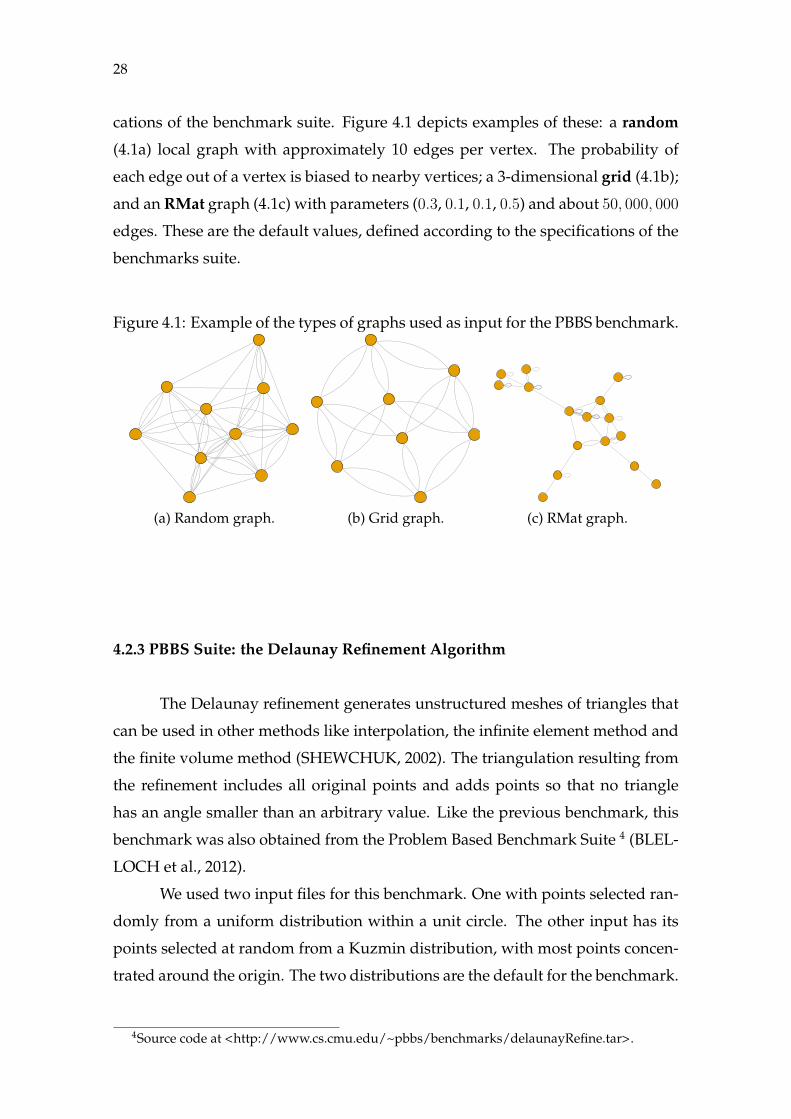
cations of the benchmark suite. Figure 4.1 depicts examples of these: a random

(4.1a) local graph with approximately 10 edges per vertex. The probability of

each edge out of a vertex is biased to nearby vertices; a 3-dimensional grid (4.1b);

and an RMat graph (4.1c) with parameters (0.3, 0.1, 0.1, 0.5) and about 50, 000, 000

edges. These are the default values, defined according to the specifications of the

benchmarks suite.

Figure 4.1: Example of the types of graphs used as input for the PBBS benchmark.

(a) Random graph. (b) Grid graph. (c) RMat graph.

4.2.3 PBBS Suite: the Delaunay Refinement Algorithm

The Delaunay refinement generates unstructured meshes of triangles that

can be used in other methods like interpolation, the infinite element method and

the finite volume method (SHEWCHUK, 2002). The triangulation resulting from

the refinement includes all original points and adds points so that no triangle

has an angle smaller than an arbitrary value. Like the previous benchmark, this

benchmark was also obtained from the Problem Based Benchmark Suite 4 (BLEL-

LOCH et al., 2012).

We used two input files for this benchmark. One with points selected ran-

domly from a uniform distribution within a unit circle. The other input has its

points selected at random from a Kuzmin distribution, with most points concen-

trated around the origin. The two distributions are the default for the benchmark.

4Source code at <http://www.cs.cmu.edu/~pbbs/benchmarks/delaunayRefine.tar>.

29

4.3 Experimental Results and Analysis

The experimental analysis presented in this section uses ANOVA to com-

pare the results. In all tables showing the analysis of variance (ANOVA) of the

impact of frequency changes on the different metrics analyzed (energy consump-

tion, runtime, and energy-delay product), the regions marked in bold are statisti-

cally relevant at a significance level of 5%. The results shown in the format a ± b

have a as the average value and b as the standard error, which is defined as the

standard deviation of the samples divided by the square root of the number of

samples. The number of samples depends on the step of our methodology and

the benchmark. All the plots shown in this section, with the exception of the main

effects plots, show the average and the standard error of the experiments. The

plots showing the Pareto front use one standard error for the horizontal axis and

another for the vertical axis. Whenever energy-delay product (EDP) is mentioned

it refers to the equation presented in Chapter 2. In all plots and tables presented

in this section, a − symbol on the horizontal axis means the low clock frequency

is used for the region, whereas a + symbol means the high clock frequency is

used.

4.3.1 Analysis of the Graph5000 Benchmark

We divided the Graph500 benchmark in 19 parallel regions, covering all

parallel loops. This benchmark is costly in terms of computational time, with

each execution requiring about 40 seconds to execute. A full factorial design with

the 219 = 524288 combinations of slow and fast frequencies for each region and

30 replications would require 174, 762 hours to execute, which would be unfeasi-

ble. Following our methodology, instead of the full factorial we use a screening

design first to detect which regions have the most impact energy and runtime.

For this screening design we use 32 runs with 5 replications each. We opted for

32 runs because that is the lowest number of runs necessary for 19 factors with

the Plackett-Burman design. The number of replications can be low as the vari-

ability, for a given run, of runtime and energy consumption is relatively low. The

screening required 1.6 hours to execute and resulted in the selection of 3 of the

19 regions for the full factorial design. The full factorial uses 23 = 8 runs and 30

30

repetitions, taking 2.5 hours to execute.

Step #1: Screening

Figure 4.2 shows the main effects plot (MEPlot) for energy consumption.

The vertical axis shows how executing each region on low and high frequency

affects energy. The − and + symbols on the horizontal axis indicate, respectively,

the use of low or high frequency for that region. An increasing slope from the −

point to the + point of a region means energy consumption is greater with the use

of the high frequency for that region. An decreasing slope means the contrary:

energy consumption is lower with the high frequency. If the slope is zero, the use

of high or low frequency for that region does not affect energy consumption.

Regions F and K are shown as the most promising for reducing energy

consumption, and both are statistically significant at a confidence interval of 95%.

Of the regions less affected by changes on the clock frequency, C is the only that

was considered statistically significant, as shown in Table 4.2. The upward slope

indicates these three regions should consume less energy when running at the

low clock frequency than at the high clock frequency, which indicates DVFS can

improve the energy consumption of this application if the frequency is lowered

for these code regions. Energy consumption was not significantly affected by the

clock frequency used in the other regions.

Figure 4.2: MEPlot for energy consumption of the Graph500 benchmark.

A

ener

gy

− +

2500

2600

2700

B

− +

C

− +

D

− +

E

− +

F

− +

G

− +

H

− +

I

− +

J

− +

K

− +

L

− +

M

− +

N

− +

O

− +

P

− +

Q

− +

R

− +

S

− +

Regions F , J and K have the greatest effect on runtime, as illustrated in

the main effects plot shown in Figure 4.3. The runtime is negatively affected by

lowering the clock frequency, as evidenced by their downward slope. Regions

F and K are the main candidates for improving energy consumption, and ap-

parently at the price of increasing the runtime. Region J seems to affect runtime

but had no significant consequences on energy. A possible explanation is that the

runtime increase for this region at the low clock frequency was relatively greater

31

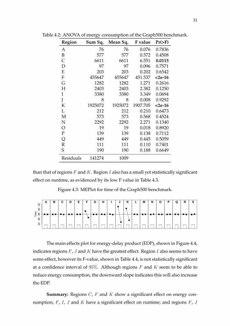
Table 4.2: ANOVA of energy consumption of the Graph500 benchmark.

Region Sum Sq. Mean Sq. F value Pr(>F)

A 76 76 0.076 0.7836B 577 577 0.572 0.4508C 6611 6611 6.551 0.0115D 97 97 0.096 0.7571E 203 203 0.202 0.6542F 455647 455647 451.537 <2e-16G 1282 1282 1.271 0.2616H 2403 2403 2.382 0.1250I 3380 3380 3.349 0.0694J 8 8 0.008 0.9292K 1925072 1925072 1907.705 <2e-16L 212 212 0.210 0.6473M 573 573 0.568 0.4524N 2292 2292 2.271 0.1340O 19 19 0.018 0.8920P 139 139 0.138 0.7112Q 449 449 0.445 0.5059R 111 111 0.110 0.7401S 190 190 0.188 0.6649

Residuals 141274 1009

than that of regions F and K. Region I also has a small yet statistically significant

effect on runtime, as evidenced by its low F value in Table 4.3.

Figure 4.3: MEPlot for time of the Graph500 benchmark.

A

Tim

e

− +

3436

3840

42

B

− +

C

− +

D

− +

E

− +

F

− +

G

− +

H

− +

I

− +

J

− +

K

− +

L

− +

M

− +

N

− +

O

− +

P

− +

Q

− +

R

− +

S

− +

The main effects plot for energy-delay product (EDP), shown in Figure 4.4,

indicates regions F , J and K have the greatest effect. Region I also seems to have

some effect, however its F-value, shown in Table 4.4, is not statistically significant

at a confidence interval of 95%. Although regions F and K seem to be able to

reduce energy consumption, the downward slope indicates this will also increase

the EDP.

Summary: Regions C, F and K show a significant effect on energy con-

sumption; F , I , J and K have a significant effect on runtime; and regions F , J

32

Table 4.3: ANOVA of runtime of the Graph500 benchmark.

Region Sum Sq. Mean Sq. F value Pr(>F)

A 0.0 0.0 0.104 0.7478B 0.1 0.1 0.165 0.6853C 0.7 0.7 2.037 0.1558D 0.1 0.1 0.166 0.6839E 0.0 0.0 0.017 0.8958F 288.2 288.2 849.458 <2e-16G 0.0 0.0 0.124 0.7250H 0.0 0.0 0.118 0.7321I 1.8 1.8 5.417 0.0214J 1650.4 1650.4 4863.798 <2e-16K 935.3 935.3 2756.513 <2e-16L 0.1 0.1 0.293 0.5892M 0.1 0.1 0.311 0.5780N 0.7 0.7 2.105 0.1490O 0.0 0.0 0.058 0.8101P 0.2 0.2 0.600 0.4399Q 0.1 0.1 0.344 0.5583R 0.3 0.3 0.970 0.3263S 0.7 0.7 2.207 0.1396

Residuals 47.5 0.3

Figure 4.4: MEPlot for the energy-delay product of the Graph500 benchmark.

A

ED

P

− +9000

01e

+05

1100

00 B

− +

C

− +

D

− +

E

− +

F

− +

G

− +

H

− +

I

− +

J

− +

K

− +

L

− +

M

− +

N

− +

O

− +

P

− +

Q

− +

R

− +

S

− +

and K on EDP.

Step #2: Full Factorial Design

Following our methodology, a full factorial experimental design was exe-

cuted for all combinations of low and high clock frequency for regions F , J and

K to better understand how they impact performance and energy consumption.

This design has 23 runs, with 30 replications each, for a total of 240 executions,

requiring 2.5 hours to execute.

We compare five of the eight versions of the benchmark: high frequency,

which executes all regions at 2.3 GHz, the highest frequency available on the pro-

33

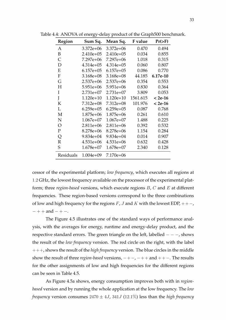
Table 4.4: ANOVA of energy-delay product of the Graph500 benchmark.

Region Sum Sq. Mean Sq. F value Pr(>F)

A 3.372e+06 3.372e+06 0.470 0.494B 2.410e+05 2.410e+05 0.034 0.855C 7.297e+06 7.297e+06 1.018 0.315D 4.314e+05 4.314e+05 0.060 0.807E 6.157e+05 6.157e+05 0.086 0.770F 3.168e+08 3.168e+08 44.185 6.17e-10G 2.537e+06 2.537e+06 0.354 0.553H 5.951e+06 5.951e+06 0.830 0.364I 2.731e+07 2.731e+07 3.809 0.053J 1.120e+10 1.120e+10 1561.615 < 2e-16K 7.312e+08 7.312e+08 101.976 < 2e-16L 6.259e+05 6.259e+05 0.087 0.768M 1.875e+06 1.875e+06 0.261 0.610N 1.067e+07 1.067e+07 1.488 0.225O 2.811e+06 2.811e+06 0.392 0.532P 8.278e+06 8.278e+06 1.154 0.284Q 9.834e+04 9.834e+04 0.014 0.907R 4.531e+06 4.531e+06 0.632 0.428S 1.678e+07 1.678e+07 2.340 0.128

Residuals 1.004e+09 7.170e+06

cessor of the experimental platform; low frequency, which executes all regions at

1.2 GHz, the lowest frequency available on the processor of the experimental plat-

form; three region-based versions, which execute regions B, C and E at different

frequencies. These region-based versions correspond to the three combinations

of low and high frequency for the regions F , J and K with the lowest EDP, ++−,

−+ + and −+−.

The Figure 4.5 illustrates one of the standard ways of performance anal-

ysis, with the averages for energy, runtime and energy-delay product, and the

respective standard errors. The green triangle on the left, labelled − − −, shows

the result of the low frequency version. The red circle on the right, with the label

+++, shows the result of the high frequency version. The blue circles in the middle

show the result of three region-based versions,−+−,−++ and ++−. The results

for the other assignments of low and high frequencies for the different regions

can be seen in Table 4.5.

As Figure 4.5a shows, energy consumption improves both with in region-

based version and by running the whole application at the low frequency. The low

frequency version consumes 2470 ± 4J , 341J (12.1%) less than the high frequency

34

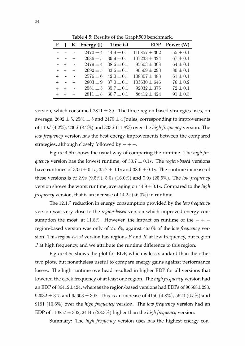
Table 4.5: Results of the Graph500 benchmark.

F J K Energy (J) Time (s) EDP Power (W)

- - - 2470± 4 44.9± 0.1 110857± 302 55± 0.1- - + 2686± 5 39.9± 0.1 107233± 324 67± 0.1- + - 2479± 4 38.6± 0.1 95603± 308 64± 0.1- + + 2692± 5 33.6± 0.1 90569± 293 80± 0.1

+ - - 2576± 6 42.0± 0.1 108307± 483 61± 0.1+ - + 2803± 9 37.0± 0.1 103630± 646 76± 0.2+ + - 2581± 5 35.7± 0.1 92032± 375 72± 0.1+ + + 2811± 8 30.7± 0.1 86412± 424 91± 0.3

version, which consumed 2811 ± 8J . The three region-based strategies uses, on

average, 2692 ± 5, 2581 ± 5 and 2479 ± 4 Joules, corresponding to improvements

of 119J (4.2%), 230J (8.2%) and 333J (11.8%) over the high frequency version. The

low frequency version has the best energy improvements between the compared

strategies, although closely followed by −+−.

Figure 4.5b shows the usual way of comparing the runtime. The high fre-

quency version has the lowest runtime, of 30.7 ± 0.1s. The region-based versions

have runtimes of 33.6± 0.1s, 35.7± 0.1s and 38.6± 0.1s. The runtime increase of

these versions is of 2.9s (9.5%), 5.0s (16.0%) and 7.9s (25.5%). The low frequency

version shows the worst runtime, averaging on 44.9± 0.1s. Compared to the high

frequency version, that is an increase of 14.2s (46.0%) in runtime.

The 12.1% reduction in energy consumption provided by the low frequency

version was very close to the region-based version which improved energy con-

sumption the most, at 11.8%. However, the impact on runtime of the − + −

region-based version was only of 25.5%, against 46.0% of the low frequency ver-

sion. This region-based version has regions F and K at low frequency, but region

J at high frequency, and we attribute the runtime difference to this region.

Figure 4.5c shows the plot for EDP, which is less standard than the other

two plots, but nonetheless useful to compare energy gains against performance

losses. The high runtime overhead resulted in higher EDP for all versions that

lowered the clock frequency of at least one region. The high frequency version had

an EDP of 86412±424, whereas the region-based versions had EDPs of 90568±293,

92032 ± 375 and 95603 ± 308. This is an increase of 4156 (4.8%), 5620 (6.5%) and

9191 (10.6%) over the high frequency version. The low frequency version had an

EDP of 110857± 302, 24445 (28.3%) higher than the high frequency version.

Summary: The high frequency version uses has the highest energy con-

35

Figure 4.5: Average energy consumption, runtime and energy-delay product asa function of different strategies of frequency configurations for the Graph500benchmark.

0

2400260028003000

−−− −+− −++ ++− +++Strategy

Ene

rgy

(J)

(a) Energy.

0

30

35

40

45

−−− −+− −++ ++− +++Strategy

Tim

e (s

)

(b) Runtime.

0

8000090000

100000110000

−−− −+− −++ ++− +++Strategy

Ene

rgy−

dela

y pr

oduc

t

(c) Energy-delay product.

sumption, 2811± 8J , the lowest runtime, 30.7± 0.1s, and the lowest EDP, 86412±

424. The low frequency version uses the least amount of energy, 2470 ± 4J , has

the highest runtime, 44.9 ± 0.1s, and the highest EDP, 110857 ± 302. The + + −

region-based version consumes 2692± 5J , executes in 33.6± 0.1s, and has an EDP

of 90568±293. The−++ region-based version consumes 2581±5J , takes 35.7±0.1s

to execute and has an EDP of 92032 ± 375. The − + − region-based version con-

sumes almost the same as the low frequency version, 2479 ± 4J , takes less time to

execute, 38.6 ± 0.1s, and has an EDP of 95603 ± 308, lower than the EDP of the

high frequency version but lower than the EDP of low frequency.

Step #3: Pareto Analysis

The Pareto front shown in Figure 4.6a, and zoomed-in in Figure 4.6b, is

made up by five points, the high and low clock frequency versions and the same

three points we used in the traditional analysis shown in the previous step: ++−,

−++ and−+−. The points are averages of the 30 repetitions. The standard error

for time is shown by a horizontal error bar, and the standard error for energy is

shown by a vertical error bar. The signs below the points in Figure 4.6b represent

the frequency used for each of the three regions, F , J and K. A + sign means the

region was executed at the high clock frequency, 2.3GHz, and a− sign means the

region was executed at the low clock frequency, 1.2GHz. The leftmost point in the

front, represented by a red circle and which has the lowest runtime and highest

energy consumption, is the high frequency version (+ + +). The rightmost point,

represented by a green triangle and with the highest runtime and the lowest en-

36

ergy consumption, is the low frequency version (−−−). The points between these

two points, represented by blue squares, are the different region-based versions.

Looking at the first sign, which corresponds to the frequency used for re-

gion F , we can see flipping it results in a improvement of 120J and an increase

of 3s in the runtime. Similarly, the third sign (K) reduces energy consumption

by 230J and increases runtime by 5s. The middle sign (J), however, only reduces

energy consumption by 10J , while increasing the runtime by 6s. Even though the

low frequency version is part of the Pareto front, there is little advantage of using

that version over the region-based version that runs all regions at low frequency

except for J . The low frequency version saves 8.4J more than the−+− version but

with an increase of 6.3s in runtime, showing that region-based version provides al-

most the same energy savings with a much lower runtime penalty. Compared

to the traditional approach, shown in Figures 4.5a and 4.5b, the Pareto approach

makes the differences in runtime and energy consumption between the different

versions easier to observe, even when there is a large number of versions being

compared.

Figure 4.6: Energy-runtime Pareto front of the Graph500 benchmark.

0

245026502850

0 30 35 40 45Time (s)

Ene

rgy

(J)

High Frequency

Low Frequency

Region−based

(a) Overview.

+++

++−

−+−

+−−

−−−

−++

+−+

−−+

2450

2550

2650

2750

2850

30 35 40 45Time (s)

Ene

rgy

(J)

High Frequency

Low Frequency

Region−based

(b) Zoom.

The Pareto front for power and runtime, shown in Figure 4.7a, and zoomed-

in in Figure 4.7b, is comprised of six of the eight versions analysed. All points

shown are the average result for 30 repetitions. The vertical and horizontal error

bars show the standard error for runtime and power, respectively. The high fre-

quency version, represented as the red circle on the top left, has the highest power

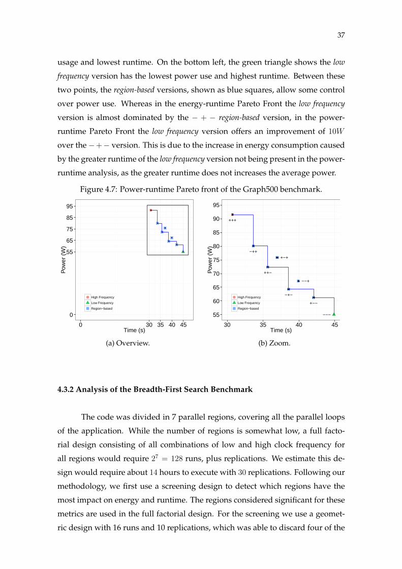
37

usage and lowest runtime. On the bottom left, the green triangle shows the low

frequency version has the lowest power use and highest runtime. Between these

two points, the region-based versions, shown as blue squares, allow some control

over power use. Whereas in the energy-runtime Pareto Front the low frequency

version is almost dominated by the − + − region-based version, in the power-

runtime Pareto Front the low frequency version offers an improvement of 10W

over the−+− version. This is due to the increase in energy consumption caused

by the greater runtime of the low frequency version not being present in the power-

runtime analysis, as the greater runtime does not increases the average power.

Figure 4.7: Power-runtime Pareto front of the Graph500 benchmark.

0

55

65

75

85

95

0 30 35 40 45Time (s)

Pow

er (

W)

High Frequency

Low Frequency

Region−based

(a) Overview.

+++

++−

−+−

+−−

−−−

−+++−+

−−+

55

60

65

70

75

80

85

90

95

30 35 40 45Time (s)

Pow

er (

W)

High Frequency

Low Frequency

Region−based

(b) Zoom.

4.3.2 Analysis of the Breadth-First Search Benchmark

The code was divided in 7 parallel regions, covering all the parallel loops

of the application. While the number of regions is somewhat low, a full facto-

rial design consisting of all combinations of low and high clock frequency for

all regions would require 27 = 128 runs, plus replications. We estimate this de-

sign would require about 14 hours to execute with 30 replications. Following our

methodology, we first use a screening design to detect which regions have the

most impact on energy and runtime. The regions considered significant for these

metrics are used in the full factorial design. For the screening we use a geomet-

ric design with 16 runs and 10 replications, which was able to discard four of the

38

seven regions. The screening took around 3 hours to execute, and the full factorial

took about one hour.

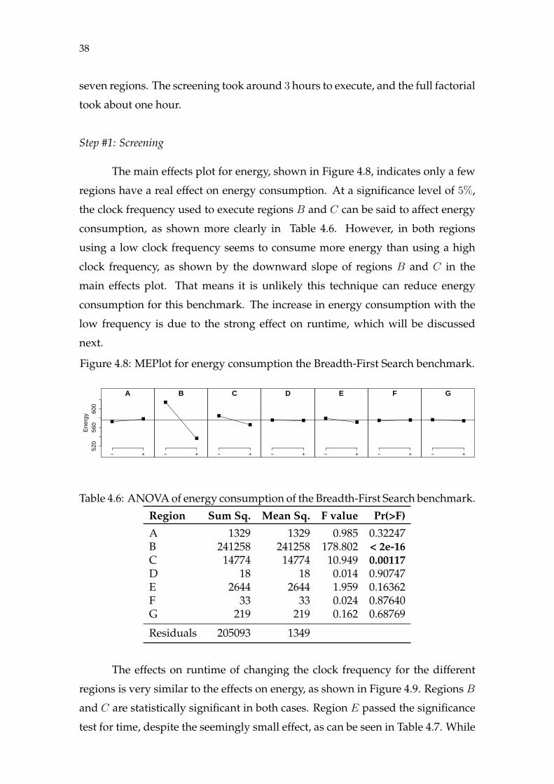
Step #1: Screening

The main effects plot for energy, shown in Figure 4.8, indicates only a few

regions have a real effect on energy consumption. At a significance level of 5%,

the clock frequency used to execute regions B and C can be said to affect energy

consumption, as shown more clearly in Table 4.6. However, in both regions

using a low clock frequency seems to consume more energy than using a high

clock frequency, as shown by the downward slope of regions B and C in the

main effects plot. That means it is unlikely this technique can reduce energy

consumption for this benchmark. The increase in energy consumption with the

low frequency is due to the strong effect on runtime, which will be discussed

next.

Figure 4.8: MEPlot for energy consumption the Breadth-First Search benchmark.

A

Ene

rgy

− +

520

560

600

B

− +

C

− +

D

− +

E

− +

F

− +

G

− +

Table 4.6: ANOVA of energy consumption of the Breadth-First Search benchmark.

Region Sum Sq. Mean Sq. F value Pr(>F)

A 1329 1329 0.985 0.32247B 241258 241258 178.802 < 2e-16C 14774 14774 10.949 0.00117D 18 18 0.014 0.90747E 2644 2644 1.959 0.16362F 33 33 0.024 0.87640G 219 219 0.162 0.68769

Residuals 205093 1349

The effects on runtime of changing the clock frequency for the different

regions is very similar to the effects on energy, as shown in Figure 4.9. Regions B

and C are statistically significant in both cases. Region E passed the significance

test for time, despite the seemingly small effect, as can be seen in Table 4.7. While

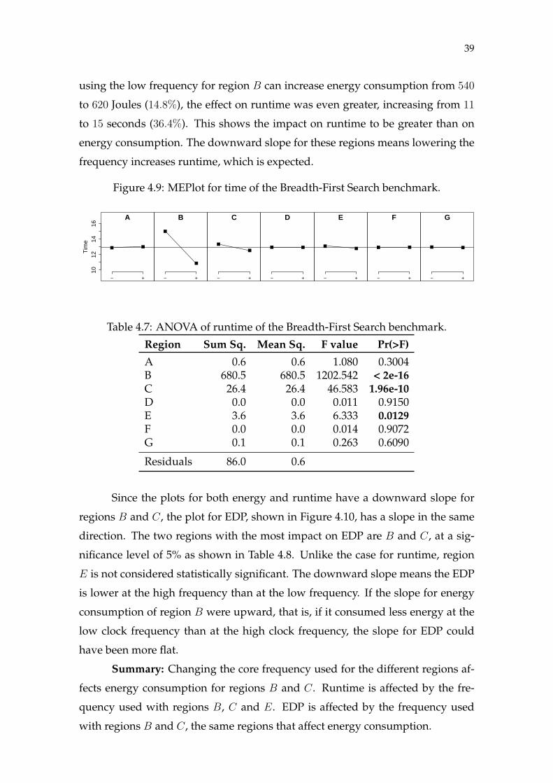
39

using the low frequency for region B can increase energy consumption from 540

to 620 Joules (14.8%), the effect on runtime was even greater, increasing from 11

to 15 seconds (36.4%). This shows the impact on runtime to be greater than on

energy consumption. The downward slope for these regions means lowering the

frequency increases runtime, which is expected.

Figure 4.9: MEPlot for time of the Breadth-First Search benchmark.

A

Tim

e

− +

1012

1416

B

− +

C

− +

D

− +

E

− +

F

− +

G

− +

Table 4.7: ANOVA of runtime of the Breadth-First Search benchmark.

Region Sum Sq. Mean Sq. F value Pr(>F)

A 0.6 0.6 1.080 0.3004B 680.5 680.5 1202.542 < 2e-16C 26.4 26.4 46.583 1.96e-10D 0.0 0.0 0.011 0.9150E 3.6 3.6 6.333 0.0129F 0.0 0.0 0.014 0.9072G 0.1 0.1 0.263 0.6090

Residuals 86.0 0.6

Since the plots for both energy and runtime have a downward slope for

regions B and C, the plot for EDP, shown in Figure 4.10, has a slope in the same

direction. The two regions with the most impact on EDP are B and C, at a sig-

nificance level of 5% as shown in Table 4.8. Unlike the case for runtime, region

E is not considered statistically significant. The downward slope means the EDP

is lower at the high frequency than at the low frequency. If the slope for energy

consumption of region B were upward, that is, if it consumed less energy at the

low clock frequency than at the high clock frequency, the slope for EDP could

have been more flat.

Summary: Changing the core frequency used for the different regions af-

fects energy consumption for regions B and C. Runtime is affected by the fre-

quency used with regions B, C and E. EDP is affected by the frequency used

with regions B and C, the same regions that affect energy consumption.

40

Figure 4.10: MEPlot for the energy-delay product of the Breadth-First Searchbenchmark.

A

ED

P

− +

5500

7000

8500

B

− +

C

− +

D

− +

E

− +

F

− +

G

− +

Table 4.8: ANOVA of energy-delay product of the Breadth-First Search bench-mark.

Region Sum Sq. Mean Sq. F value Pr(>F)

A 1675773 1675773 1.342 0.248552B 465628510 465628510 372.801 < 2e-16C 18677903 18677903 14.954 0.000163D 57542 57542 0.046 0.830335E 3896886 3896886 3.120 0.079344F 213095 213095 0.171 0.680150G 407045 407045 0.326 0.568928

Residuals 189847893 1248999

Step #2: Full Factorial Design

Following our methodology, we use the screening to select the regions to

use with the more expensive full factorial design. It should be noted that for

this benchmark the screening already indicates no energy savings will obtained.

Regions B, C and E were selected for use with the full factorial design. Our full

factorial design uses 23 = 8 runs and 30 replications for each of the 3 input graphs,

for a total of 720 executions, requiring about one hour to run.

The traditional results use three versions of the benchmark: high frequency,

which executes all regions at 2.3 GHz, the highest frequency available on the

processor of the experimental platform; low frequency, which executes all regions

at 1.2 GHz, the lowest frequency available on the processor of the experimental

platform; region-based, which executes regions B and C at 2.4 GHz and region E at

1.2 GHz. We chose which regions to run at high or low frequency as to minimize

the energy-delay product.

The average energy, runtime and energy-delay product for the three strate-

gies described above are shown in Figure 4.11, along with the standard error. The

green triangle on the left, with the label − − −, represents the low frequency ver-

41

sion. On the right, represented by the red circle and labelled + + +, is shown the

high frequency version. The blue square, in the center and with the label + + −

represents the region-based version. The results for other assignments of low and

high frequencies are shown in Table 4.9.

Table 4.9: Results of the Breadth-First Search benchmark.

B C E Energy (J) Time (s) EDP Power (W)

- - - 644± 13 15.9± 0.2 10357± 412 40± 0.2- - + 627± 5 15.4± 0.1 9688± 161 41± 0.0- + - 598± 4 14.5± 0.1 8707± 103 41± 0.0- + + 604± 11 14.4± 0.2 8778± 307 42± 0.2

+ - - 551± 4 11.5± 0.1 6337± 108 48± 0.0+ - + 541± 3 11.1± 0.1 6024± 61 49± 0.0+ + - 524± 4 10.5± 0.1 5512± 88 50± 0.0+ + + 521± 4 10.3± 0.1 5385± 88 51± 0.0

The energy results are shown in Figure 4.11a. The high frequency version

uses the least amount of energy, 521 ± 4 Joules. This shows that for this bench-

mark a race to finish strategy, that tries to finish the computation as soon as pos-

sible, fares better than the other analysed options in terms of energy savings.

The region-based version uses slightly more energy than the high frequency ver-

sion, 524±4 Joules, increasing energy use by 0.5%. The low frequency version uses

the highest amount of energy, 644± 13 Joules, 23.6% more than the high frequency

version.

Figure 4.11: Average energy consumption, runtime and energy-delay product asa function of different strategies of frequency configurations for the Breadth-FirstSearch benchmark.

0

500

650

−−− ++− +++Strategy

Ene

rgy

(J)

(a) Energy.

0

10

16

−−− ++− +++Strategy

Tim

e (s

)

(b) Runtime.

0

5000

11000

−−− ++− +++Strategy

Ene

rgy−

dela

y pr

oduc

t

(c) Energy-delay product.

The runtime results can be seen in Figure 4.11b. The high frequency ver-

sion has the lowest runtime, 10.3 ± 0.1 seconds. The region-based version has a

42

very close runtime, 10.5 ± 0.1 seconds, an increase of 1.8%. Meanwhile, the low

frequency version has a runtime of 15.9 ± 0.2, 54.5% more than the high frequency

version.

Figure 4.11c compares the EDP of the different versions. Since the high

frequency version has lower execution time and energy consumption, it also has

the lowest EDP, 5385±88. The EDP for the region-based version is almost the same,

5512± 88, an increase of 2.3%. As for the low frequency version, since it has higher

runtime and energy consumption its EDP is also much higher: 10357±412, 92.3%

greater than the high frequency version.

Summary: The high frequency version has the lowest energy consumption,

521 ± 4J , lowest runtime, 10.3 ± 0.1s, and, consequently, lowest EDP, 5385 ± 88.

The low frequency version has the highest energy consumption, 644± 13J , highest

runtime, 15.9 ± 0.2s, and highest EDP, 10357 ± 412. The region-based has very

similar results to the high frequency version, with 524±4J of energy consumption,

execution time of 10.5± 0.1s, and an EDP of 5512± 88.

Step #3: Pareto Analysis

Figures 4.12a and 4.12b show an alternative to the classical methodology

of comparing energy efficiency. However, in this benchmark the Pareto front is

made of only one point. This is because one of the versions compared has the

best values for both time and energy. The values shown are averages for the 30

executions, and the horizontal and vertical error bars show the standard error

for time and energy, respectively. The red circle at the bottom left, which is the

only point in the Pareto front, corresponds to the high frequency version. The green

triangle on the top right is the low frequency version, and ranks last in both runtime

and energy consumption. The blue squares are the region-based with different

regions executing at the low and high frequency, and rank between the high and

low frequency versions on both runtime and energy. The pluses and minuses close

to each point describe if the high or low frequency was used for the regions B,

C and E, respectively. These results were expected from the main effects plot for

energy, displayed in Figure 4.8, and which shows none of the selected regions can

improve energy consumption by running at the low frequency.

Compared to the traditional analysis, shown in Figures 4.11a and 4.11b,

the Pareto approach makes it much easier to notice the effects of each of the par-

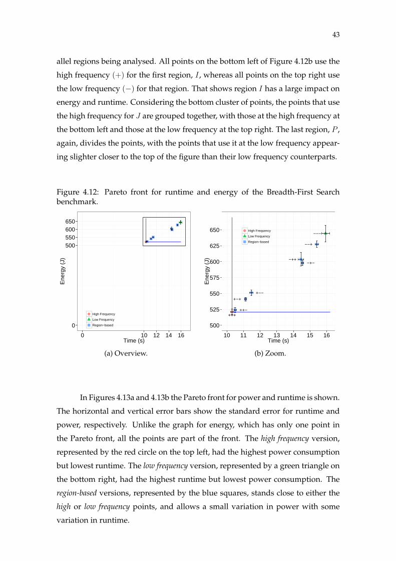
43

allel regions being analysed. All points on the bottom left of Figure 4.12b use the

high frequency (+) for the first region, I , whereas all points on the top right use

the low frequency (−) for that region. That shows region I has a large impact on

energy and runtime. Considering the bottom cluster of points, the points that use

the high frequency for J are grouped together, with those at the high frequency at

the bottom left and those at the low frequency at the top right. The last region, P ,

again, divides the points, with the points that use it at the low frequency appear-

ing slighter closer to the top of the figure than their low frequency counterparts.

Figure 4.12: Pareto front for runtime and energy of the Breadth-First Searchbenchmark.

0

500550600650

0 10 12 14 16Time (s)

Ene

rgy

(J)

High Frequency

Low Frequency

Region−based

(a) Overview.

+++++−

−+−

+−−

−−−

+−+

−−+

−++

500

525

550

575

600

625

650

10 11 12 13 14 15 16Time (s)

Ene

rgy

(J)

High Frequency

Low Frequency

Region−based

(b) Zoom.

In Figures 4.13a and 4.13b the Pareto front for power and runtime is shown.

The horizontal and vertical error bars show the standard error for runtime and

power, respectively. Unlike the graph for energy, which has only one point in

the Pareto front, all the points are part of the front. The high frequency version,

represented by the red circle on the top left, had the highest power consumption

but lowest runtime. The low frequency version, represented by a green triangle on

the bottom right, had the highest runtime but lowest power consumption. The

region-based versions, represented by the blue squares, stands close to either the

high or low frequency points, and allows a small variation in power with some

variation in runtime.

44

Figure 4.13: Pareto front for runtime and power of the Breadth-First Search bench-mark.

0

40

45

50

0 10 12 14 16Time (s)

Pow

er (

W)

High Frequency

Low Frequency

Region−based

(a) Overview.

+++

++−

−+−

+−−

−−−

+−+

−−+

−++

40

42

44

46

48

50

10 11 12 13 14 15 16Time (s)

Pow

er (

W)

High Frequency

Low Frequency

Region−based

(b) Zoom.

4.3.3 Analysis of the Delaunay Refinement Benchmark

The code was divided into 16 parallel regions, covering all parallel regions

of the code. A full factorial experiment, using all combinations of low and high

clock frequency for all regions, would require 216 = 65535 runs, ignoring repli-

cations. Supposing 30 replications, such design would require 4023 hours to exe-

cute. Following our methodology, instead of using a full factorial design with all

the regions we first filter out the less important regions with the use of a screening

design. The screening design has 64 runs with 10 replications each, taking little

more than one hour to execute. The full factorial design uses three regions and

requires half an hour to run.

Step #1: Screening

As illustrated in Figure 4.14, region I has the greatest impact on energy

consumption. Furthermore, it shows an upward slope. That means the energy

used at the low frequency is lower than at the high frequency, making I a good

candidate to improve energy consumption. Regions N and P also have an up-

ward slope, however Table 4.10 shows them to be statistically irrelevant at a sig-

nificance level of 5%. The other regions, A, B, C, D, E, F , G, H , J , K, L, M and

O, had no statistically significant effect on energy.

45

Figure 4.14: MEPlot for the energy consumption of the Delaunay benchmark.

A

Ene

rgy

− +

550

560

570

580 B

− +

C

− +

D

− +

E

− +

F

− +

G

− +

H

− +

I

− +

J

− +

K

− +

L

− +

M

− +

N

− +

O

− +

P

− +

Table 4.10: ANOVA of energy reduction effect of the Delaunay benchmark.

Region Sum Sq. Mean Sq. F value Pr(>F)

A 22408 22408 1.312 0.25248B 4672 4672 0.274 0.60115C 937 937 0.055 0.81488D 98 98 0.006 0.93972E 33756 33756 1.976 0.16027F 14510 14510 0.850 0.35704G 11832 11832 0.693 0.40555H 11799 11799 0.691 0.40620I 115648 115648 6.771 0.00948J 29955 29955 1.754 0.18588K 25445 25445 1.490 0.22271L 27159 27159 1.590 0.20778M 14720 14720 0.862 0.35357N 63906 63906 3.742 0.05352O 32538 32538 1.905 0.16800P 47355 47355 2.773 0.09639

Residuals 10640552 17080

Regions I and J have the greatest effect on runtime, as shown in Fig-

ure 4.15. As the slope goes downward, running these regions at the low frequency

should result in longer execution times than at the high frequency.Moreover,

these two regions are statistically significant at a significance level of 5%, as shown

in Table 4.11. The other regions seem to only affect runtime slightly, if at all.

Figure 4.15: MEPlot for time of the Delaunay benchmark.

A

Tim

e

− +

6.8

7.2

7.6

8

B

− +

C

− +

D

− +

E

− +

F

− +

G

− +

H

− +

I

− +

J

− +

K

− +

L

− +

M

− +

N

− +

O

− +

P

− +

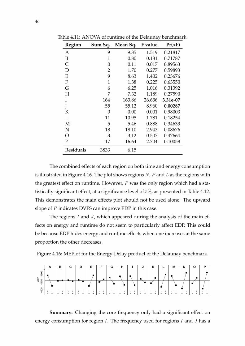
46

Table 4.11: ANOVA of runtime of the Delaunay benchmark.

Region Sum Sq. Mean Sq. F value Pr(>F)

A 9 9.35 1.519 0.21817B 1 0.80 0.131 0.71787C 0 0.11 0.017 0.89563D 2 1.70 0.277 0.59893E 9 8.63 1.402 0.23676F 1 1.38 0.225 0.63550G 6 6.25 1.016 0.31392H 7 7.32 1.189 0.27590I 164 163.86 26.636 3.31e-07J 55 55.12 8.960 0.00287K 0 0.00 0.001 0.98003L 11 10.95 1.781 0.18254M 5 5.46 0.888 0.34633N 18 18.10 2.943 0.08676O 3 3.12 0.507 0.47664P 17 16.64 2.704 0.10058

Residuals 3833 6.15

The combined effects of each region on both time and energy consumption

is illustrated in Figure 4.16. The plot shows regions N , P and L as the regions with

the greatest effect on runtime. However, P was the only region which had a sta-

tistically significant effect, at a significance level of 5%, as presented in Table 4.12.

This demonstrates the main effects plot should not be used alone. The upward

slope of P indicates DVFS can improve EDP in this case.

The regions I and J , which appeared during the analysis of the main ef-

fects on energy and runtime do not seem to particularly affect EDP. This could

be because EDP hides energy and runtime effects when one increases at the same

proportion the other decreases.

Figure 4.16: MEPlot for the Energy-Delay product of the Delaunay benchmark.

A

ED

P

− +

4000

4400

4800

B

− +

C

− +

D

− +

E

− +

F

− +

G

− +

H

− +

I

− +

J

− +

K

− +

L

− +

M

− +

N

− +

O

− +

P

− +

Summary: Changing the core frequency only had a significant effect on

energy consumption for region I . The frequency used for regions I and J has a

47

Table 4.12: ANOVA of energy-delay product of the Delaunay benchmark.

Region Sum Sq. Mean Sq. F value Pr(>F)

A 4.157e+07 41573317 1.623 0.2031B 6.213e+04 62134 0.002 0.9607C 3.899e+05 389894 0.015 0.9018D 7.624e+05 762385 0.030 0.8631E 4.208e+07 42081246 1.643 0.2004F 2.405e+06 2404912 0.094 0.7594G 1.442e+07 14421125 0.563 0.4533H 2.759e+07 27594059 1.077 0.2997I 3.022e+07 30222911 1.180 0.2778J 4.631e+06 4630960 0.181 0.6708K 1.040e+07 10401670 0.406 0.5242L 5.889e+07 58885448 2.299 0.1300M 3.316e+07 33156883 1.295 0.2556N 9.351e+07 93507811 3.651 0.0565O 1.194e+07 11935401 0.466 0.4951P 9.935e+07 99353287 3.879 0.0493

Residuals 1.596e+10 25611875

significant effect on execution time. EDP was significantly affected only by the

frequency used for region P .

Step #2: Full Factorial Design

Following our methodology, we selected the most promising regions for

use with the full factorial design. The selected regions are I , J and P . The full

factorial design has 23 = 8 runs with 30 replications each, adding up to a total of

240 executions.

For presenting the results in the traditional way we use three versions of

the Delaunay Refinement benchmark: high frequency, which executes all regions

at 2.3 GHz, the highest frequency available on the processor of the experimen-

tal platform; low frequency, which executes all regions at 1.2 GHz, the lowest

frequency available on the processor of the experimental platform; region-based,

which executes regions I and J at 1.2 GHz and P at 2.3 GHz. The regions in the

last strategy were chosen as to minimize the energy-delay product.

Figure 4.17 shows three plots (from left to right) with the average values of

the energy, runtime and energy-delay product as a function of the three different

strategies previously described for the traditional analysis. The green triangle on

48

the left, labelled−−−, represents the low frequency version. The blue square in the

middle, with the label−−+, represents the region-based version. The red circle on

the right, labelled +++ represents the high frequency version. The results for other

assignments of low and high frequencies to the regions are shown in Table 4.13.

Table 4.13: Results of the Delaunay Refine benchmark.

I J P Energy (J) Time (s) EDP Power (W)

- - - 465± 3 7.5± 0.1 3478± 68 62± 0.2- - + 465± 3 7.5± 0.1 3476± 57 62± 0.2- + - 580± 5 7.3± 0.1 4247± 106 80± 0.4- + + 573± 4 7.1± 0.1 4103± 70 80± 0.3

+ - - 575± 4 7.1± 0.1 4096± 93 81± 0.4+ - + 578± 5 7.1± 0.1 4138± 106 81± 0.4+ + - 557± 7 5.9± 0.1 3338± 135 94± 0.8+ + + 545± 3 5.7± 0.1 3120± 56 96± 0.3

For energy, the Figure 4.17a shows that the high frequency version is the

worst in terms of energy used, with an average of 545 ± 3.4 Joules. The region-

based version has an average of 465± 2.9 Joules of energy consumption, 15% less

than the high frequency version. The low frequency version uses the least amount

of energy, 465 ± 3.4 Joules, practically the same as the region-based version. So

although DVFS can improve energy consumption of this benchmark, the region-

based strategy does not use less energy than running the whole application at

the low frequency. Regarding runtime, the Figure 4.17b shows the high frequency

version has the lowest execution time, 5.7 ± 3.4 seconds on average. The region-

based and the low frequency versions had very close results, 7.5±0.07 and 7.5±0.08,

respectively, which correspond to an increase of 30.6% and 30.7% over the high

frequency version. Finally, the analysis of the Energy-delay product depicted in

Figure 4.17c shows that the high frequency has the lowest EDP, 3120 ± 55.9 on

average. The region-based and the low frequency versions again had similar results,

3476 ± 56.7 and 3478 ± 68.2. These values are an increase of 11.4% over the high

frequency version.

Summary: The high frequency version has the highest energy consumption

545 ± 3.4J , the lowest runtime, 5.7 ± 3.4s and an EDP of 3120 ± 55.9. The low

frequency version uses the less energy, 465 ± 3.4J , has a longer execution time,

7.5 ± 0.08s, and a higher EDP than the high frequency version, 3478 ± 68.2. The

region-based is tied with the low frequency version, with an energy consumption of

465± 2.9J , 7.5± 0.07s of execution time, and an EDP of 3476± 56.7.

49

Figure 4.17: Average energy consumption, runtime and energy-delay product asa function of different strategies of frequency configurations for the DelaunayRefine benchmark.

0

450

550

−−− −−+ +++Strategy

Ene

rgy

(J)

(a) Energy.

0

5

6

7

8

−−− −−+ +++Strategy

Tim

e (s

)

(b) Runtime.

0

3000

3500

−−− −−+ +++Strategy

Ene

rgy−

dela

y pr

oduc

t

(c) Energy-delay product.

Step #3: Pareto Analysis

Figures 4.18a and 4.18b show an alternative to the classical methodology of

comparing energy efficiency. The values shown are averages for the 30 executions

of each combination of low frequency and high frequency regions. The standard

error is shown by the error bars. The horizontal error bars are the standard error

for time and the vertical bars for energy. The red square in the top left corre-

sponds to the version using the high clock frequency for all regions. The green

triangle on the bottom right is the opposite, all regions are executed at the low

clock frequency. The blue squares use the low clock frequency for some regions

and the high clock frequency for others. Close to the points, the labels, composed

of pluses and minuses signs, indicate the frequency used for each region. The

plus sign means the high frequency was used, whereas the minus sign means the

low frequency was used. The first sign corresponds to region I , the second to J

and the third to P . The blue line crosses the three Pareto-optimal points, which

are the high frequency version, low frequency version and the region-based version

which used the low frequency for regions I and J and high frequency for region

P .

The graph shows regions I and J worsened both energy consumption and

runtime. Region P had very little effect, as shown in point + +−, on the middle

left, which stands close to + + + but with slightly greater runtime and energy

consumption. Likewise, point − − +, on the bottom right, is indistinguishable

from − − −. These points allows for some fine-tuning when deciding which

version to use. At the same time, they simplify visualizing the results since the

50

points that are not Pareto-optimal can be ignored.

Both the Pareto and the traditional analysis, illustrated in Figures 4.17a

and 4.17b, show a large difference in runtime and energy consumption between

the low and high frequency versions. The Pareto analysis, however, makes it clear

region P has a very small effect on runtime and energy. The other two regions, I

and J , divide the points in three groups: those which use the high frequency for

both regions (+ + + and + + −), at the left; those which use the low frequency

for both regions (− − − and − − +), at the bottom right; and those that use high

frequency for one region and low frequency for the other (− + −,− + +,+ −

−and + −+, at the top right. A possible reason might be that the control flow

moves between these two regions, and the use of different frequencies for them

causes a high number of frequency changes, and, consequently, a high overhead.

Figure 4.18: Pareto front for runtime and energy of the Delaunay Refine bench-mark.

0

450

500

550

600

0.0 5.5 6.5 7.5Time (s)

Ene

rgy

(J)

High Frequency

Low Frequency

Region−based

(a) Overview.

+++

−++++−

−+−

+−−

−−−

+−+

−−+

450

475

500

525

550

575

600

5.5 6.0 6.5 7.0 7.5Time (s)

Ene

rgy

(J)

High Frequency

Low Frequency

Region−based

(b) Zoom.

The Pareto front for power is shown in Figures 4.19a and 4.19b. The stan-

dard error for runtime and power is shown, respectively, by the horizontal and

vertical error bars. Like the energy curve, + + + and + + − are very close to-

gether at the top left, while − − − and − − + are in the bottom right. However,

unlike in the energy curve, the other points are now part of the Pareto front. As

such, while the region-based strategy could not reduce energy consumption on

this benchmark, it provided a middle ground for power consumption, although

with a very high and negative effect on runtime.

51

Figure 4.19: Pareto front for runtime and power of the Delaunay Refine bench-mark.

0

60

80

100

0.0 5.5 6.5 7.5Time (s)

Pow

er (

W)

High Frequency

Low Frequency

Region−based

(a) Overview.

+++

−++

++−

−+−

+−−

−−−

+−+

−−+60

80

100

5.5 6.0 6.5 7.0 7.5Time (s)

Pow

er (

W)

High Frequency

Low Frequency

Region−based

(b) Zoom.

52

5 CONCLUSION

The work described in this dissertation presents a performance analysis

evaluation methodology for finding the best code-regions for improving energy

consumption through changes in the CPU clock frequency. The proposal is three-

fold: (a) a clever design of experiments based on screening that allows the quick

detection of the most important regions especially when many regions are present;

(b) a traditional energy and performance evaluation of the regions considered as

good candidates; (c) a Pareto-based analysis of the trade-off between runtime and

energy consumption.

Our proposal is validated against three benchmarks. In the Graph500

benchmark the region-based approach obtained an improvement of 12.1% in en-

ergy consumption when compared with the high frequency execution. The energy

gain of the region-based is very similar to the one obtained with the low frequency

version. However, the execution time overhead of the region-based was only 25.7%

larger than high frequency, while in the low frequency the overhead is 47.3% larger.

For the other two benchmarks, BFS and Delaunay Refine, our methodology de-

tected unsatisfactory results for the region-based approach. For BFS, for example,

we have observed that lowering the frequency increases energy consumption. In

the Delaunay Refine, the region-based approach shows similar results to the low

frequency.

The use of screening, which reduces the number of experiments necessary

for the full factorial, resulted in 4.1 hours running experiments for the Graph500

benchmark, against 174 thousand hours which would be required for a full fac-

torial experiment with all the factors. In the BFS experiment, the use of screening

reduced the experimental time necessary from 14 hours to 4 hours. The Delau-

nay Refine experiment 1.7 hour were required, against the 4 thousand hours that

a full factorial experiment would take. This shows the screening technique can

save a high amount of experimental time when many factors are being consid-

ered, which is often the case on the beginning of a performance evaluation.

Future work includes the automatic annotation of parallel regions, and a

comparison of the conclusions obtained through our methodology against the

conclusions that would be obtained with a traditional performance and energy

evaluation.

53

REFERENCES

BALAPRAKASH, P.; TIWARI, A.; WILD, S. Multi objective optimization of hpckernels for performance, power, and energy. In: JARVIS, S. A.; WRIGHT, S. A.;HAMMOND, S. D. (Ed.). High Performance Computing Systems. PerformanceModeling, Benchmarking and Simulation. [S.l.]: Springer InternationalPublishing, 2014, (Lecture Notes in Computer Science, v. 8551). p. 239–260. ISBN978-3-319-10213-9.

BLELLOCH, G. E. et al. Internally deterministic parallel algorithms can be fast.SIGPLAN Not., ACM, New York, NY, USA, v. 47, n. 8, p. 181–192, feb. 2012.ISSN 0362-1340.

BOX, G. E.; HUNTER, J. S.; HUNTER, W. G. Statistics for experimenters: design,innovation, and discovery. AMC, v. 10, p. 12, 2005.

BROOKS, D. et al. Power-aware microarchitecture: design and modelingchallenges for next-generation microprocessors. Micro, IEEE, v. 20, n. 6, p. 26–44,Nov 2000. ISSN 0272-1732.

CHAKRABARTI, D.; ZHAN, Y.; FALOUTSOS, C. R-mat: A recursive model forgraph mining. In: SIAM. SDM. [S.l.], 2004. v. 4, p. 442–446.

CHOI, K.; SOMA, R.; PEDRAM, M. Fine-grained dynamic voltage and frequencyscaling for precise energy and performance tradeoff based on the ratio of off-chipaccess to on-chip computation times. Computer-Aided Design of IntegratedCircuits and Systems, IEEE Transactions on, IEEE, v. 24, n. 1, p. 18–28, 2005.

CHOI, K.; SOMA, R.; PEDRAM, M. Fine-grained dynamic voltage and frequencyscaling for precise energy and performance tradeoff based on the ratio of off-chipaccess to on-chip computation times. Computer-Aided Design of IntegratedCircuits and Systems, IEEE Transactions on, v. 24, n. 1, p. 18–28, Jan 2005. ISSN0278-0070.

COMMITTEE, G. . S. Graph500 Specification. 2010. <http://www.graph500.org/specifications>.

DAVIS, J. D. et al. No Hardware Required: Building and ValidatingComposable Highly Accurate OS-based Power Models. [S.l.], 2011.

DONGARRA, J.; LUSZCZEK, P. Linpack benchmark. In: Encyclopedia ofParallel Computing. [S.l.]: Springer, 2011. p. 1033–1036.

DONGARRA, J.; LUSZCZEK, P. Linpack benchmark. In: PADUA, D. (Ed.).Encyclopedia of Parallel Computing. [S.l.]: Springer US, 2011. p. 1033–1036.ISBN 978-0-387-09765-7.

EHRGOTT, M. Multicriteria Optimization. 1999.

FENG, W. chun; CAMERON, K. The green500 list: Encouraging sustainablesupercomputing. Computer, v. 40, n. 12, p. 50–55, Dec 2007. ISSN 0018-9162.

54

GE, R. et al. Cpu miser: A performance-directed, run-time system for power-aware clusters. In: IEEE. Parallel Processing, 2007. ICPP 2007. InternationalConference on. [S.l.], 2007. p. 18–18.

GE, R. et al. Powerpack: Energy profiling and analysis of high-performancesystems and applications. Parallel and Distributed Systems, IEEE Transactionson, v. 21, n. 5, p. 658–671, May 2010. ISSN 1045-9219.

GELLER, T. Supercomputing exaflop target. In: Comm. of the ACM. [S.l.]: ACMNew York, NY, USA, 2011. p. 54(8).

HOROWITZ, M.; INDERMAUR, T.; GONZALEZ, R. Low-power digital design.In: Low Power Electronics, 1994. Digest of Technical Papers., IEEE Symposium.[S.l.: s.n.], 1994. p. 8–11.

HSU, C.-H.; FENG, W.-c. A feasibility analysis of power awareness incommodity-based high-performance clusters. In: IEEE. Cluster Computing,2005. IEEE International. [S.l.], 2005. p. 1–10.

HSU, C.-h.; FENG, W.-c. A power-aware run-time system for high-performancecomputing. In: IEEE COMPUTER SOCIETY. Proceedings of the 2005 ACM/IEEEconference on Supercomputing. [S.l.], 2005. p. 1.

INTEL. Intel 64 and IA-32 Architectures Software Developer’s Manual -Volume 3B. [S.l.], 2013.

KIM, K. H.; BUYYA, R.; KIM, J. Power aware scheduling of bag-of-tasksapplications with deadline constraints on dvs-enabled clusters. In: Proceedingsof the Seventh IEEE International Symposium on Cluster Computing and theGrid. Washington, DC, USA: IEEE Computer Society, 2007. (CCGRID ’07), p.541–548. ISBN 0-7695-2833-3.

KIM, W. et al. System level analysis of fast, per-core dvfs using on-chip switchingregulators. In: High Performance Computer Architecture, 2008. HPCA 2008.IEEE 14th International Symposium on. [S.l.: s.n.], 2008. p. 123–134. ISSN1530-0897.

LAWSON, G.; SOSONKINA, M.; SHEN, Y. Energy evaluation for applicationswith different thread affinities on the intel xeon phi. In: Computer Architectureand High Performance Computing Workshop (SBAC-PADW), 2014International Symposium on. [S.l.: s.n.], 2014. p. 54–59.

LIM, M.; FREEH, V. W.; LOWENTHAL, D. Adaptive, transparent frequencyand voltage scaling of communication phases in mpi programs. In: SC 2006Conference, Proceedings of the ACM/IEEE. [S.l.: s.n.], 2006. p. 14–14.

MEISNER, D.; WENISCH, T. Peak power modeling for data center serverswith switched-mode power supplies. In: Low-Power Electronics and Design(ISLPED), 2010 ACM/IEEE International Symposium on. [S.l.: s.n.], 2010. p.319–324.

MEUER, H. et al. Top500. 2014. <http://www.top500.org>.

55

MONTGOMERY, D. C. Design and analysis of experiments. [S.l.]: John Wiley &Sons, 2008.

MURPHY, R. C. et al. Introducing the graph 500. Cray User’s Group (CUG),2010.

NVIDIA. NVIDIA Management Library (NVML). [S.l.], 2012.

PADOIN, E. et al. Saving energy by exploiting residual imbalances on iterativeapplications. In: High Performance Computing (HiPC), 21st InternationalConference on. Goa, India: [s.n.], 2014. p. 1–10.

RAJOVIC, N. et al. The low power architecture approach towards exascalecomputing. Journal of Computational Science, Elsevier, v. 4, n. 6, p. 439 – 443,2013. ISSN 1877-7503.

ROUNTREE, B. et al. Adagio: Making dvs practical for complex hpc applications.In: Proceedings of the 23rd International Conference on Supercomputing.New York, NY, USA: ACM, 2009. (ICS ’09), p. 460–469. ISBN 978-1-60558-498-0.

SCARAMELLA, J. Worldwide server power and cooling expense 2006-2010forecast. International Data Corporation (IDC), 2006.

SHEWCHUK, J. R. Delaunay refinement algorithms for triangular meshgeneration. Comput. Geom. Theory Appl., Elsevier Science Publishers B. V.,Amsterdam, The Netherlands, The Netherlands, v. 22, n. 1-3, p. 21–74, may 2002.ISSN 0925-7721.

SHUN, J. et al. Brief announcement: The problem based benchmark suite. In:Proceedings of the Twenty-fourth Annual ACM Symposium on Parallelism inAlgorithms and Architectures. New York, NY, USA: ACM, 2012. (SPAA ’12), p.68–70. ISBN 978-1-4503-1213-4.

SIMPSON, T. et al. Metamodels for computer-based engineering design: Surveyand recommendations. Engineering with Computers, Springer-Verlag, v. 17,n. 2, p. 129–150, 2001. ISSN 0177-0667.

SUBRAMANIAM, B. et al. Green500. 2014. <http://www.green500.org>.

SUEUR, E. L.; HEISER, G. Dynamic voltage and frequency scaling: The lawsof diminishing returns. In: Proceedings of the 2010 International Conferenceon Power Aware Computing and Systems. Berkeley, CA, USA: USENIXAssociation, 2010. (HotPower’10), p. 1–8.

TORRELLAS, J. Architectures for extreme-scale computing. Computer, IEEE,v. 42, n. 11, p. 28–35, 2009.

VASIc, N. et al. Making cluster applications energy-aware. In: Proceedings ofthe 1st Workshop on Automated Control for Datacenters and Clouds. NewYork, NY, USA: ACM, 2009. (ACDC ’09), p. 37–42. ISBN 978-1-60558-585-7.

VOGELEER, K. D. et al. The energy/frequency convexity rule: Modeling andexperimental validation on mobile devices. CoRR, abs/1401.4655, 2014.