A parallel particle swarm optimization and enhanced sparrow ...

A parallel particle swarm optimization andenhanced sparrow search algorithm for unmannedaerial vehicle path planningZiwei Wang  ( [email protected] )

Foshan University

Research Article

Keywords: enhanced sparrow search algorithm, particle swarm optimization, unmanned aerial vehicle,path planning

Posted Date: March 3rd, 2022

DOI: https://doi.org/10.21203/rs.3.rs-1375515/v1

License: This work is licensed under a Creative Commons Attribution 4.0 International License.  Read Full License

A parallel particle swarm optimization and enhanced

sparrow search algorithm for unmanned aerial vehicle path

planning

Ziwei Wanga*

aFoshan University, Guangdong, China. *Corresponding author. Email address: [email protected] (Ziwei Wang).

Abstract: The path planning problem is that Unmanned aerial vehicle (UAV) needs to plan a feasible path from the starting point to the end point in a specific environment. But it cannot get satisfactory results using ordinary algorithms, to solve this problem, a hybrid algorithm named as PESSA is proposed, where particle swarm optimization (PSO) and an enhanced sparrow search algorithm (ESSA) work in parallel. In the ESSA, the random jump of the producer’s position is strengthened to guarantee the global search ability, each scrounger keeps learning from the optimal experience of the producers, and for the sparrow with the optimal position, when it perceives the danger, the difference between the best individual and the worst individual will be imposed to speed up the search process. And then, the elite reverse search strategy was added to increase the diversity of the population. In this paper, the performance of PESSA is verified by 10 basic functions, the experimental results illustrate that PESSA is better compared with other twelve algorithms. Finally, the proposed PESSA is applied in 4 different scenarios including two groups of 2D environments and two groups of 3D environments. The results show that the PESSA algorithm can acquire more feasible and effective route than compared algorithms.

Keywords: enhanced sparrow search algorithm, particle swarm optimization, unmanned aerial vehicle, path planning.

1.Introduction

UAV is a kind of aircraft without pilot in the cabin that can fly autonomously based on preprogrammed flight plans. As a modern aviation equipment, unmanned aerial vehicle (UAV) has attracted much attention because of its potential to work in complex and dangerous environments [1]. Path planning is an important task in UAV mission planning system. It is necessary to obtain a safe and efficient path from initial position to target under specific constraints [2]. Therefore, the nature of path planning is a complex optimization problem, which can be solved by efficient algorithms.

In recent years, a series of path planning algorithms have been proposed. In order to improve the stability and efficiency of path planning methods in complex environments, the literature [3] presented a RETRBG algorithm, a robust and efficient trajectory replanning method based on the guiding path. The literature [4] introduced CPP method based on a Region Optimal Decomposition (ROD), which achieved good results when applied to the path planning of UAV in

a port environment. The literature [5] proposed a new diving planning method based on the original underwater pathfinding algorithm, which considers safety constraints and maximizes the number of points of interest (POIs) visited. The literature [6] proposed a 3D UAV path planning framework, which takes into account the semantic attributes of the environment and user-specified airspace constraints, and designs detailed and complete small-scale 3D reconstruction. Graph-based is one kind of such effective methods, including Voronoi diagram searching method [7], A-star search and D-star lite search [8][9] etc. The Voronoi diagram divides the map into several small pieces that contain only one threatening convex polygon. They all use an Eppstein’s k-best algorithm [10] to find the optimal path, but it is difficult to consider the motion constraints of UAV, which means it usually cannot be used in practical situations [11]. The performance constraints of the UAV itself also need to be considered when designing the flight path of the UAV. In order to take the motion constraints of UAV into account during the planning process, Ref. [12] proposed the sparse A* search (SAS) algorithm to plan a real-time route for aircraft. Because all kinds of path constraints are considered in the planning process, SAS algorithm can prune the search space effectively. In order to improve the durability of USV, a feasible path planning method for USV based on ocean current data considering energy consumption was proposed [13]. This method combines Voronoi diagram, Visibility graph, Dijkstra's search and energy consumption function, so that USVs can avoid obstacles with minimal energy.

It is generally accepted that meta-heuristic algorithms are an efficient and effective optimization technique and has been used as a viable candidate to solve path planning problems. Ref. [7] presented a novel multi-frequency vibrational genetic algorithm (mVGA) to solve the UAV path planning problem. Ref. [14] proposed a modified differential evolution (DE) method to acquire a feasible route to solve the global route planning problem for UAV. In [15], a novel multi-UAV path planning model is developed which is based on the time stamp segmentation (TSS) that utilizes the common time bases to simplify the handling of multi-UAV coordination cost and a novel social-class pigeon-inspired optimization (SCPIO) algorithm is proposed as the solver of optimal search on the TSS model. Ref. [16] proposed an adaptive selective variation constrained differential evolution algorithm for UAV path planning in disaster scenarios. Ref. [17] presents a three-dimensional path planning algorithm based on adaptive sensitivity decision operator combined with particle swarm optimization (PSO) technique, which constructed an adaptive sensitivity decision region and overcame the shortcomings of local optimization and slow convergence. Ref. [18] solves the problems of low search efficiency and poor convergence accuracy in 3D path planning by combining BAS algorithm with three non-trivial mechanisms, including local quick search, ant colony algorithm initial path generation and search information orientation. Ref. [11] presents a hybrid differential evolution (DE) with quantum-behaved particle swarm optimization (QPSO) denoted as DEQPSO for the UAV route planning on the sea. An improved cuckoo search algorithm based on compact and parallel techniques for three-dimensional path planning problems is proposed in [19]. In reference [20], a spherical vector based particle swarm optimization algorithm (SPSO) was proposed to solve the path planning problem of unmanned aerial vehicles (UAVs) in complex environments under multiple threats. Literature [21] uses GWO algorithm to solve the path planning problem of 3-D UAV, which provides the direction for the subsequent readers. Ref. [22] proposes an algorithm based on improved quantum particle swarm optimization (QPSO), which can plan a UAV path more quickly and accurately. Ref. [23] propose an algorithm based on the well-known PSO algorithm,

in which the UAV team follows the networking approach known as Delay Tolerant Network. In recent years, researchers have turned their attention to the technology of algorithm

hybridization, which is the combination of two or more meta heuristic optimization algorithms [24][25]. In this technology, a good combination of algorithms can show more effective optimization when dealing with practical problems [26]. A new methodology is proposed in literature [27] to determine the optimal trajectory of the path for multi-robot in a clutter environment using hybridization of improved particle swarm optimization (IPSO) with an improved gravitational search algorithm (IGSA). The literature [11] presents a hybrid differential evolution (DE) with quantum-behaved particle swarm optimization (QPSO) for the unmanned aerial vehicle (UAV) route planning on the sea. In [28], a new algorithm called HSGWO-MSOS for UAV path planning is proposed. The new algorithm combines the simplified grey wolf optimization algorithm (SGWO) with the improved symbiotic biological search algorithm (MSOS). Ref. [29] proposed an improved algorithm GEDGWO, which combined the basic GWO and GED strategy, and applied it to solve the urban tracking path planning problem of multi-UAV and multi-target.

Xue [30] propose a novel swarm intelligence optimization technique based on Sparrow's behavior of foraging and evading predator which is called sparrow search algorithm (SSA). The proposed SSA can provide highly competitive results compared with the other state-of-the-art algorithms in terms of searching precision, convergence speed, and stability. However, SSA just like most other intelligent optimization algorithms, it easily falls into premature and local optimal algorithms and it has not been applied in 3D UAV path planning. So, this paper will introduce an improved sparrow search algorithm for UAV path planning named PESSA. PESSA algorithm is run in parallel by PSO algorithm and ESSA algorithm, and the better one is the final result. The ESSA algorithm is an enhanced version of SSA algorithm. We have mainly made the following adjustments, first, for producers, we change the random jump of their position to random move, which increases the stability of the search range and the ability of global search. Then, for scroungers, we only retain their ability to follow producers and plunder food. Finally, for the sparrows who perceive the danger, when it is in the current optimal position, we let the sparrows randomly jump to a random position between the global optimal position and the worst position, and make it walk randomly to get close to other sparrows. In PESSA, we also introduce the elite reverse search strategy to improve the ability of the algorithm to jump out of the local optimum.

The main work of this paper are summarized as follows: This paper presents an improved algorithm ESSA based on SSA algorithm (Enhanced

sparrow search algorithm). This paper proposes a parallel ESSA algorithm and an improved PSO algorithm PESSA, and

carries out elite reverse search based on it, which improves the ability of the algorithm to jump out of local optimization.

The PESSA algorithm is applied to UAV path planning problem and compared with two basic algorithms and better experimental results are obtained. The structure of this paper is as follows. In the section 2, DEM map data is extracted,

obstacles are simulated, and the environment of UAV path planning is modeled. In the section 3, a new algorithm PESSA is proposed, and PSO algorithm and SSA algorithm are briefly introduced. In the section 4, the new algorithm is applied to the environment model are proposed in Section 2. The performance of the new algorithm is comprehensively verified through different environments,

and the effectiveness of the new algorithm is proved by comparing with other algorithms. The last part is the summary of the thesis.

2. Mathematical model in UAV path planning

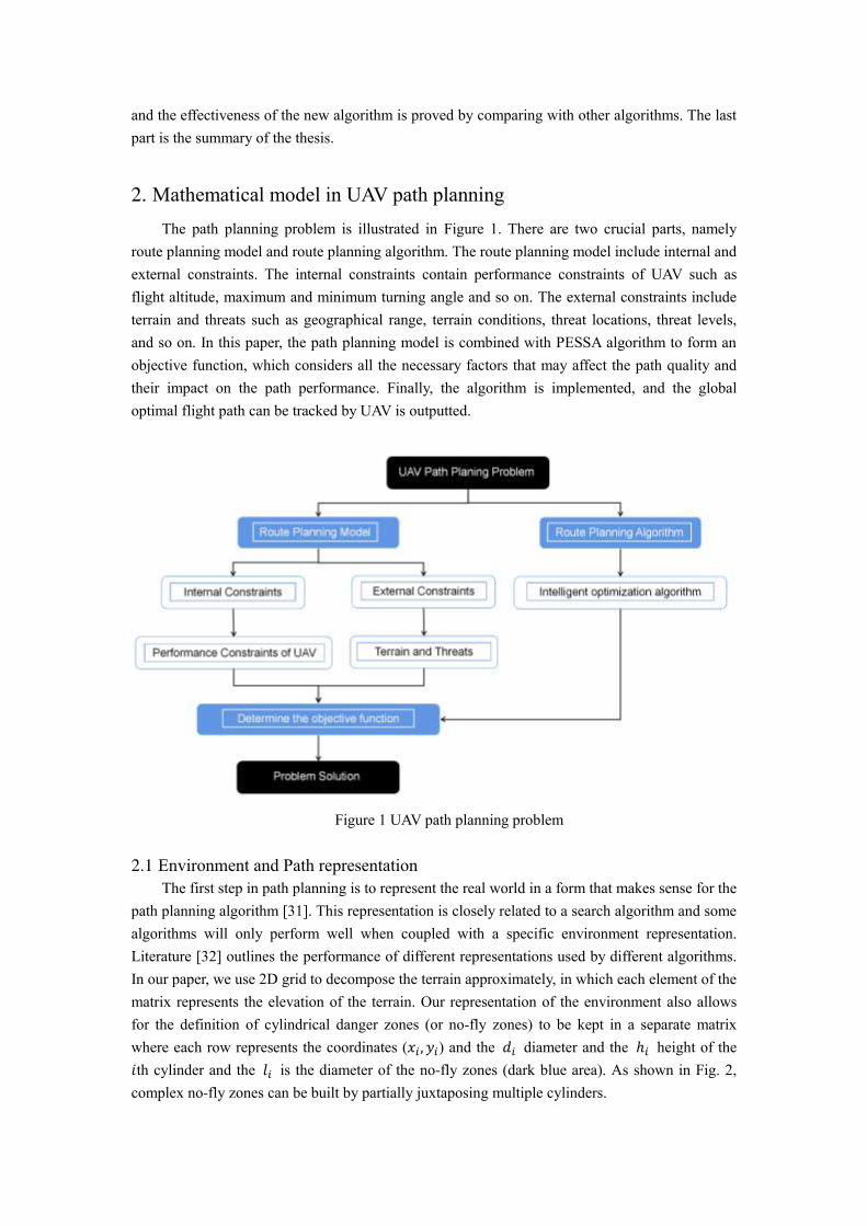
The path planning problem is illustrated in Figure 1. There are two crucial parts, namely route planning model and route planning algorithm. The route planning model include internal and external constraints. The internal constraints contain performance constraints of UAV such as flight altitude, maximum and minimum turning angle and so on. The external constraints include terrain and threats such as geographical range, terrain conditions, threat locations, threat levels, and so on. In this paper, the path planning model is combined with PESSA algorithm to form an objective function, which considers all the necessary factors that may affect the path quality and their impact on the path performance. Finally, the algorithm is implemented, and the global optimal flight path can be tracked by UAV is outputted.

Figure 1 UAV path planning problem

2.1 Environment and Path representation

The first step in path planning is to represent the real world in a form that makes sense for the path planning algorithm [31]. This representation is closely related to a search algorithm and some algorithms will only perform well when coupled with a specific environment representation. Literature [32] outlines the performance of different representations used by different algorithms. In our paper, we use 2D grid to decompose the terrain approximately, in which each element of the matrix represents the elevation of the terrain. Our representation of the environment also allows for the definition of cylindrical danger zones (or no-fly zones) to be kept in a separate matrix where each row represents the coordinates (𝑥𝑖 , 𝑦𝑖) and the 𝑑𝑖 diameter and the ℎ𝑖 height of the 𝑖th cylinder and the 𝑙𝑖 is the diameter of the no-fly zones (dark blue area). As shown in Fig. 2, complex no-fly zones can be built by partially juxtaposing multiple cylinders.

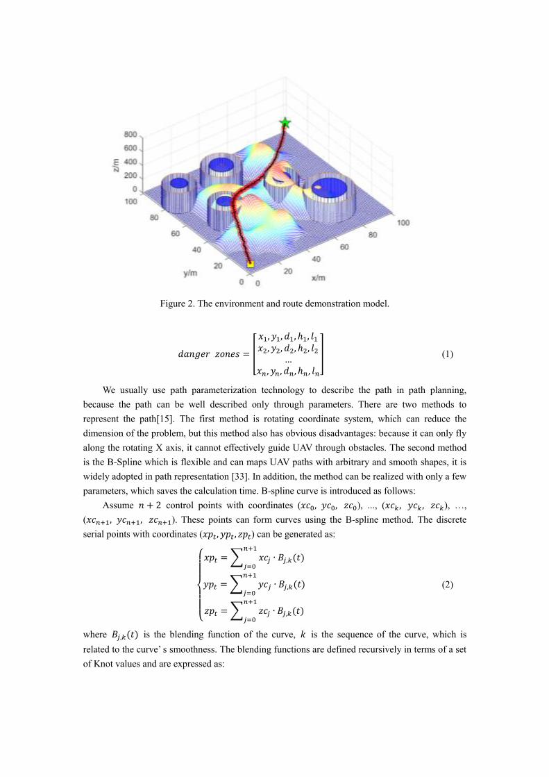
Figure 2. The environment and route demonstration model.

𝑑𝑎𝑛𝑔𝑒𝑟 𝑧𝑜𝑛𝑒𝑠 = [ 𝑥1, 𝑦1, 𝑑1, ℎ1, 𝑙1𝑥2, 𝑦2, 𝑑2, ℎ2, 𝑙2…𝑥𝑛, 𝑦𝑛, 𝑑𝑛, ℎ𝑛, 𝑙𝑛] (1)

We usually use path parameterization technology to describe the path in path planning, because the path can be well described only through parameters. There are two methods to represent the path[15]. The first method is rotating coordinate system, which can reduce the dimension of the problem, but this method also has obvious disadvantages: because it can only fly along the rotating X axis, it cannot effectively guide UAV through obstacles. The second method is the B-Spline which is flexible and can maps UAV paths with arbitrary and smooth shapes, it is widely adopted in path representation [33]. In addition, the method can be realized with only a few parameters, which saves the calculation time. B-spline curve is introduced as follows:

Assume 𝑛 + 2 control points with coordinates (𝑥𝑐0, 𝑦𝑐0, 𝑧𝑐0), ..., (𝑥𝑐𝑘 , 𝑦𝑐𝑘 , 𝑧𝑐𝑘), …, (𝑥𝑐𝑛+1, 𝑦𝑐𝑛+1, 𝑧𝑐𝑛+1). These points can form curves using the B-spline method. The discrete serial points with coordinates (𝑥𝑝𝑡, 𝑦𝑝𝑡 , 𝑧𝑝𝑡) can be generated as:

{ 𝑥𝑝𝑡 =∑ 𝑥𝑐𝑗 ∙ 𝐵𝑗,𝑘(𝑡)𝑛+1𝑗=0𝑦𝑝𝑡 =∑ 𝑦𝑐𝑗 ∙ 𝐵𝑗,𝑘(𝑡)𝑛+1𝑗=0𝑧𝑝𝑡 =∑ 𝑧𝑐𝑗 ∙ 𝐵𝑗,𝑘(𝑡)𝑛+1𝑗=0

(2)

where 𝐵𝑗,𝑘(𝑡) is the blending function of the curve, 𝑘 is the sequence of the curve, which is related to the curve’ s smoothness. The blending functions are defined recursively in terms of a set of Knot values and are expressed as:

𝐵𝑗,1(𝑡)= { 1 𝑖𝑓 𝐾𝑛𝑜𝑡(𝑗) ≤ 𝑡 ≤ 𝐾𝑛𝑜𝑡(𝑗 + 1) 1 𝑖𝑓 𝐾𝑛𝑜𝑡(𝑗) ≤ 𝑡 ≤ 𝐾𝑛𝑜𝑡(𝑗 + 1) 𝑎𝑛𝑑 𝑡 = 𝑛 − 𝑘 + 30 𝑜𝑡ℎ𝑒𝑟𝑤𝑖𝑠𝑒

(3)

𝐵𝑗,𝑘(𝑡) = (𝑡 − 𝐾𝑛𝑜𝑡(𝑗)) × 𝐵𝑗,𝑘−1(𝑡)𝐾𝑛𝑜𝑡(𝑗 + 𝑘 − 1) − 𝐾𝑛𝑜𝑡(𝑗) + 𝐾𝑛𝑜𝑡(𝑖 + 𝑘 − 1) × 𝐵𝑖+1,𝑘−1(𝑡)𝐾𝑛𝑜𝑡(𝑗 + 𝑘) − 𝐾𝑛𝑜𝑡(𝑗 + 1)

(4)

{𝐾𝑛𝑜𝑡(𝑗) = 0 𝑖𝑓 𝑗 < 𝑘 𝐾𝑛𝑜𝑡(𝑗) = 𝑗 − 𝑘 + 1 𝑖𝑓 𝑘 ≤ 𝑗 ≤ 𝑛𝐾𝑛𝑜𝑡(𝑗) = 𝑛 − 𝑘 + 2 𝑖𝑓 𝑛 < 𝑗

(5)

where 𝑡 varies from 0 to 𝑛 − 𝑘 + 3 in constant steps, which offers a series of discrete points [34].

2.2 Objective function design

Objective function determines the feasibility of the proposed algorithm and the following elements are taken into account.

(1) Effects of path length

Due to the limited fuel carried by UAV, its flight distance should be as short as possible. Through the B-Spline curve, the path can be represented as a series of discrete points, such as (𝑝0, 𝑝1, … , 𝑝𝑘 , … , 𝑝𝑛+1). The coordinates of 𝑝𝑘 are (𝑥𝑝𝑘, 𝑦𝑝𝑘, 𝑧𝑝𝑘) which is a discrete point representing the current position of the UAV, 𝑝0 is the starting point and 𝑝𝑛+1 is the ending point i.e. Generally, the shorter the distance, the less time is required. The distance can be calculated by the Euclidean operator as follows: 𝑓𝑙𝑒𝑛𝑔𝑡ℎ = 1 − (𝐿𝑥𝑝0𝑥𝑝𝑛+1𝐿𝑡𝑟𝑢𝑒 ) (6)

where 𝐿𝑥𝑝0𝑥𝑝𝑛+1 is the length of the straight line connecting the starting point 𝑥𝑝0 and the end point 𝑥𝑝𝑛+1. The 𝐿𝑡𝑟𝑢𝑒 is the actual length of the trajectory, it’ s calculation method is as follows:

𝐿𝑡𝑟𝑢𝑒 =∑√(𝑥𝑝𝑘+1 − 𝑥𝑝𝑘)2 + (𝑦𝑝𝑘+1 − 𝑦𝑝𝑘)2 + (𝑧𝑝𝑘+1 − 𝑧𝑝𝑘)2𝑛𝑘=0 (7)

where 𝑘 is the index of discrete points from 0 to 𝑛. (2) Effects of flight altitude

In order to prevent enemy radar detection, flying at low altitude is safer than flying at high altitude. However, in order to reduce the risk of hitting mountains during low flying, the flight altitude needs to be kept within a certain criterion. In our model, the minimum and maximum flight altitudes are set respectively. When the UAV flies in this range, it is the best. When it exceeds this range, it needs to be punished.

𝑓𝑎𝑙𝑡𝑖={ ∑ (1 − ℎ𝑚𝑖𝑛𝑧𝑝𝑖 − 𝑓(𝑥𝑝𝑖 , 𝑦𝑝𝑖))𝑛𝑖=1 𝑛 𝑧𝑝𝑖 > 𝑓(𝑥𝑝𝑖 , 𝑦𝑝𝑖) + 𝐻𝑚𝑎𝑥 0 𝑓(𝑥𝑝𝑖 , 𝑦𝑝𝑖) + 𝐻𝑚𝑖𝑛 < 𝑧𝑝𝑖 < 𝑓(𝑥𝑝𝑖 , 𝑦𝑝𝑖) + 𝐻𝑚𝑎𝑥∑ ( ℎ𝑚𝑖𝑛𝑧𝑝𝑖 − 𝑓(𝑥𝑝𝑖 , 𝑦𝑝𝑖) − 1)𝑛𝑖=1 𝑛 𝑓(𝑥𝑝𝑖 , 𝑦𝑝𝑖) ≤ 𝑧𝑝𝑖 ≤ 𝑓(𝑥𝑝𝑖 , 𝑦𝑝𝑖) + 𝐻𝑚𝑖𝑛

(8)

where (𝑥𝑝𝑖 , 𝑦𝑝𝑖 , 𝑧𝑝𝑖) is the current coordinate of UAV, 𝑓(𝑥𝑝𝑖 , 𝑦𝑝𝑖) is the terrain height at point (𝑥𝑝𝑖 , 𝑦𝑝𝑖), and 𝐻𝑚𝑖𝑛 is the permitted minimum flying height of UAV.

(3) Effects of danger zones

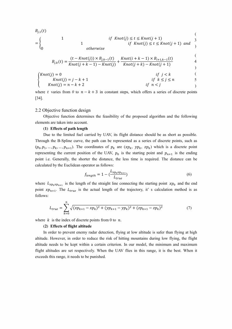
The deterministic threat is considered in this paper, such as radar, artillery, missile and so on. Once an UAV flies in the scope of threats, it has a probability to be found or taken down. We have defined a 100% danger zone in the threat zone, in which the UAV is bound to suffer damage, so the UAV cannot fly to the 100% threat zone. Here a cylinder model in space is defined as a threat area with coordinate vector 𝑑𝑎𝑛𝑔𝑒𝑟 𝑧𝑜𝑛𝑒𝑠𝑖 [𝑥𝑖 , 𝑦𝑖 , 𝑑𝑖 , ℎ𝑖 , 𝑙𝑖], where (𝑥𝑖 , 𝑦𝑖) is the center on the XOY plain, ℎ𝑖 is the covered height and 𝑑𝑖 is the diameter of cylinder bottom, 𝑙𝑖 is the diameter of the no-fly zones. A detailed diagram of the threat area is shown in Figure 3. The term associated with the violation of the danger zones for an UAV with coordinate [𝑥𝑝𝑡, 𝑦𝑝𝑡 , 𝑧𝑝𝑡] is defined as follows: 𝑓𝑑𝑎𝑛𝑔𝑒𝑟= { 0 𝑖𝑓 𝑧𝑝𝑡 > ℎ𝑖 0 𝑖𝑓 𝑧𝑝𝑡 < ℎ𝑖 , 𝑑𝑑 ≥ 𝑑𝑖/2 1 − 𝑑𝑑 − 𝑙𝑖/2(𝑑𝑖 − 𝑙𝑖)/2 𝑖𝑓 𝑧𝑝𝑡 < ℎ𝑖 , 𝑙𝑖/2 ≤ 𝑑𝑑 < 𝑑𝑖/2𝑎 𝑖𝑓 𝑧𝑝𝑡 < ℎ𝑖 , 𝑑𝑑 < 𝑙𝑖/2

(9)

where 𝑑𝑑 = √(𝑥𝑝𝑡 − 𝑥𝑖)2 + (𝑦𝑝𝑡 − 𝑦𝑖)2 is the distance between the projection point of the current UAV position on the XY plane and the threat center and 𝑎 is a relatively large constant.

Figure 3. A detailed diagram of the threat area

(4) Effects of ground collisions

In order to ensure the normal flight of UAV, our planned route cannot appear in the mountain. The term associated with ground collisions is defined as follows: 𝑓𝑔𝑟𝑜𝑢𝑛𝑑 = {0 𝐿𝑢𝑛𝑑𝑒𝑟 𝑡𝑒𝑟𝑟𝑎𝑖𝑛 = 0𝑃 𝐿𝑢𝑛𝑑𝑒𝑟 𝑡𝑒𝑟𝑟𝑎𝑖𝑛 > 0 (10)

where 𝐿𝑢𝑛𝑑𝑒𝑟 𝑡𝑒𝑟𝑟𝑎𝑖𝑛 is the total length of the subsections of the trajectory which travels below the ground level. 𝑃 is a relatively large constant.

(5) Effects of angle

The finally condition is that the angle of the UAV is limited. It should not exceed a predetermined maximum angle 𝜃𝑚𝑎𝑥. The turning angle can be calculated by these discrete points as follows:

𝑓𝑎𝑛𝑔𝑙𝑒 = {0 𝑖𝑓 𝜃 < 𝜃𝑚𝑎𝑥 𝜃 − 𝜃𝑚𝑎𝑥180 𝑜𝑡ℎ𝑒𝑟𝑤𝑖𝑠𝑒 (11)

where 𝜃 = 𝑐𝑜𝑠−1( 𝑝𝑡𝑝𝑡+1→ 𝑝𝑡𝑝𝑡−1→ ||𝑝𝑡𝑝𝑡+1|| ||𝑝𝑡𝑝𝑡−1||), and 𝑝𝑡 , 𝑝𝑡+1 are two discrete and continuous points along

the path, and the range of t is between 0 and n+1. Based on the above discussion, the UAV path planning model can be depicted as follows: 𝑓𝑜𝑏𝑗 = 𝑓𝑙𝑒𝑛𝑔𝑡ℎ + 𝑓𝑎𝑙𝑡𝑖 + 𝑓𝑑𝑎𝑛𝑔𝑒𝑟 + 𝑓𝑔𝑟𝑜𝑢𝑛𝑑 + 𝑓𝑎𝑛𝑔𝑙𝑒 (12)

3. Proposed method for global path planning

3.1 basic algorithm

3.1.1. The SSA algorithm

SSA [30] is a novel swarm optimization approach that is proposed inspired by the group wisdom, foraging and anti-predation behaviors of sparrows. In the original text, the author idealized the following behavior of the sparrows and formulated six corresponding rules. The author divides the sparrow population into producers and scroungers, and then randomly selects sparrows which are aware of the danger.

In SSA, producers with better fitness values get food preferentially in the search process. In addition, because producers are responsible for finding food and guiding the movement of the entire population. In each iteration, the location of the producer updates are as follows:

𝑋𝑖𝑗𝑡+1 = { 𝑋𝑖𝑗𝑡 ∙ exp ( −𝑖𝛼 ∙ 𝑖𝑡𝑒𝑟𝑚𝑎𝑥) 𝑖𝑓 𝑅2 < 𝑆𝑇𝑋𝑖𝑗𝑡 + 𝑄 ∙ 𝐿 𝑖𝑓 𝑅2 > 𝑆𝑇 (13)

where 𝑖=1, 2, ..., N, N denotes the swarm size, where 𝑡 represents the current iteration, 𝑗 =1, 2,… , 𝑑. 𝑋𝑖𝑗𝑡 represents the value of the 𝑗 th dimension of the 𝑖 th sparrow at iteration t. 𝑖𝑡𝑒𝑟𝑚𝑎𝑥 represents a constant with respect to the maximum number of iterations. 𝛼 ∈ (0,1] is a random number. 𝑄 is a random number that follows a normal distribution. 𝐿 shows a matrix of 1 × 𝑑 for which each element inside is 1. 𝑅2 (𝑅2 ∈ [0,1]) and 𝑆𝑇 (𝑆𝑇 ∈ [0.5,1.0]) represent the alarm value and the safety threshold respectively.

As for the scroungers, the producers are spied on by some scroungers, and when they find better food, the scroungers will immediately leave their current position to compete for food. The scrounger's position update formula is described as follows:

𝑋𝑖𝑗𝑡+1 = {𝑄 ∙ exp(𝑋𝑤𝑜𝑟𝑠𝑡𝑡 − 𝑋𝑖𝑗𝑡𝑖2 ) 𝑖𝑓 𝑖 > 𝑛/2𝑋𝑝𝑡+1 + |𝑋𝑖𝑗𝑡 −𝑋𝑝𝑡+1| ∙ 𝐴+ ∙ 𝐿 𝑜𝑡ℎ𝑒𝑟𝑤𝑖𝑠𝑒 (14)

where 𝑋𝑝 was be defined as the optimal position occupied of producers. 𝑋𝑤𝑜𝑟𝑠𝑡 is the current global worst location. 𝐴+ = 𝐴𝑇(𝐴𝐴𝑇)−1, and here 𝐴 represents a matrix of 1 × 𝑑 for which each element inside is randomly assigned 1 or −1.

The sparrows at the edge of the group quickly moved to a safe area to get a better position

when they sensed danger, while sparrows in the middle of the group walked randomly to get closer to other sparrows. The mathematical model can be expressed as:

𝑋𝑖𝑗𝑡+1 = {𝑋𝑏𝑒𝑠𝑡𝑡 + 𝛽 ∙ |𝑋𝑖𝑗𝑡 − 𝑋𝑏𝑒𝑠𝑡𝑡 | 𝑖𝑓 𝑓𝑖 > 𝑓𝑔𝑋𝑖𝑗𝑡 + 𝐾 ∙ (|𝑋𝑖𝑗𝑡 − 𝑋𝑤𝑜𝑟𝑠𝑡𝑡 |(𝑓𝑖 − 𝑓𝑤) + 𝜀 𝑖𝑓 𝑓𝑖 = 𝑓𝑔 (15)

where 𝑋𝑏𝑒𝑠𝑡𝑡 is the current global optimal location. 𝑋𝑤𝑜𝑟𝑠𝑡 denotes the current global worst location. As a step size control parameter, 𝛽 is a normal distribution of random numbers with mean value of 0 and variance of 1. 𝐾 is a random number in [-1, 1]. Here 𝑓𝑖 is the fitness value of the present sparrow, 𝑓𝑤 is the worst fitness values and 𝑓𝑔 is the current global best. 𝜀 is the smallest constant.

3.1.2. The PSO algorithm

PSO [35] is a kind of swarm intelligence optimization algorithm. Each particle 𝑖 in the swarm represents a possible solution to a problem, and is identified by a position vector 𝑋𝑖𝑑 and a velocity vector 𝑉𝑖𝑑, where 𝑖=1, 2, ..., N, N denotes the swarm size, 𝑑 is the dimension of the particle 𝑖 and 𝑑 = [1,2,… , 𝐷], 𝐷 is the dimension of the search space. Each particle updates its velocity and position by learning from its personal best experience and population best experience, the update formulas are as follows: 𝑉𝑖𝑑𝑡+1 = 𝜔𝑉𝑖𝑑𝑡 + 𝑐1𝑟1(𝑝𝑖𝑡 − 𝑋𝑖𝑑𝑡 ) + 𝑐2𝑟2(𝑋𝑏𝑒𝑠𝑡𝑡 − 𝑋𝑖𝑑𝑡 ) (16) 𝑋𝑖𝑑𝑡+1 = 𝑋𝑖𝑑𝑡 + 𝑉𝑖𝑑𝑡+1 (17) where 𝑡 represents the current iteration number, 𝑡 = 1,2,… , 𝑖𝑡𝑒𝑟𝑚𝑎𝑥 , 𝑖𝑡𝑒𝑟𝑚𝑎𝑥 represents the total iteration number, where 𝑝𝑖 denotes the personal historical best position of particle 𝑖 , 𝑋𝑏𝑒𝑠𝑡denotes the population historical best position, 𝜔 is the inertia weight, 𝑐1 and 𝑐2 are the acceleration coefficients, 𝑟1 and 𝑟2 are two uniformly distributed random numbers independently generated within [0, 1]. In addition, the velocity is limited to a certain range [𝑉𝑚𝑖𝑛, 𝑉𝑚𝑎𝑥] to prevent particles flying out of the search space, and 𝑋𝑖 ∈ [𝑋𝑚𝑖𝑛, 𝑋𝑚𝑎𝑥], where 𝑋𝑚𝑖𝑛 and 𝑋𝑚𝑎𝑥 are the lower and upper bounds of the position, respectively.

3.2. A hybrid algorithm of particle swarm optimization and enhanced sparrow algorithm

3.2.1. Enhanced sparrow search algorithm (ESSA) In SSA, producers with better fitness value get food first in the search process. In addition,

because producers are responsible for finding food and guiding the movement of the entire population. Therefore, producers can find food in a wider range of places. But in the basic SSA algorithm, when 𝑅2 > 𝑆𝑇, the producer will randomly move to the current position according to the normal distribution 𝑅2 < 𝑆𝑇, the producer multiplies a function 𝑒(−𝑖/(𝛼∙𝑖𝑡𝑒𝑟𝑚𝑎𝑥)). It is not difficult to see that the value range of this function is between [0,1], at this time, the producer's position will gradually jump to 0, which is not a good strategy for global exploration. Therefore, we change the producer's position update strategy into a step-by-step moving process, adding a standard normal distribution random number Q. the finally location of the producer is updated as below: 𝑋𝑖𝑑𝑡+1 = { 𝑋𝑖𝑑𝑡 ∙ (1 + 𝑄) 𝑖𝑓 𝑅2 < 𝑆𝑇𝑋𝑖𝑑𝑡 + 𝑄 𝑖𝑓 𝑅2 > 𝑆𝑇 (18)

where 𝑡 indicates the current iteration, 𝑡 = 1,2,… ,𝑁𝑖𝑡𝑒𝑟 , 𝑁𝑖𝑡𝑒𝑟 represents the total iteration

number. 𝑋𝑖𝑑𝑡 represents the value of the 𝑑th dimension of the 𝑖th sparrow at iteration t. 𝑅2 (𝑅2 ∈ [0,1] ) and 𝑆𝑇 (𝑆𝑇 ∈ [0.5,1.0] ) represent the alarm value and the safety threshold respectively. 𝑄 is a random number which obeys normal distribution.

As for the scroungers, they follow the producer to find food, while a group of scroungers monitor the producers, and when the producer spots something, they will show up to grab the food. But in the original SSA algorithm, when the follower is greater than 𝑛/2, the value of the scroungers are the product of a standard normal distribution random number and an exponential function based on the natural logarithm. When the population converges, its value will gradually converge to 0, which is obviously different from the strategy mentioned. Therefore, this step will be removed in our new algorithm, only the scroungers that may constantly monitor the producers and compete for food is retained. The position update formula for the scrounger is described as follows: 𝑋𝑖𝑑𝑡+1 = 𝑋𝑝𝑡+1 + |𝑋𝑖𝑑𝑡 − 𝑋𝑝𝑡+1| ∙ 𝐴+ (19) where 𝑋𝑝 is the optimal position occupied by the producer. 𝐴 represents a matrix of 1 × 𝑑 for which each element inside is randomly assigned 1 or−1, and 𝐴+ = 𝐴𝑇(𝐴𝐴𝑇)−1.

In SSA, when danger appeared, sparrows at the edge of the group moved quickly to the safety area, while sparrows in the middle of the group moved randomly to other sparrows. In the update formula of SSA algorithm, when the early-warning sparrows are at the edge of the group, they will jump to the current optimal position, that is, they will move to the safe area, in line with the rules. However, when the early-warning sparrow is in the current optimal position, it will escape to a position near itself, which is inconsistent with the rules. Therefore, when the early-warning sparrow is in the current optimal position, we let it randomly jump to a random position between the optimal position and the worst position. the mathematical model can be expressed as follows: 𝑋𝑖𝑑𝑡+1 = {𝑐 ∙ 𝑋𝑏𝑒𝑠𝑡𝑡 + 𝛽 ∙ |𝑋𝑖𝑑𝑡 − 𝑋𝑏𝑒𝑠𝑡𝑡 | 𝑖𝑓 𝑓𝑖 > 𝑓𝑔𝑐 ∙ 𝑋𝑖𝑑𝑡 + 𝛽 ∙ |𝑋𝑤𝑜𝑟𝑠𝑡𝑡 − 𝑋𝑏𝑒𝑠𝑡𝑡 | 𝑖𝑓 𝑓𝑖 = 𝑓𝑔 (20)

where 𝑋𝑏𝑒𝑠𝑡 is the current global optimal location. 𝑋𝑤𝑜𝑟𝑠𝑡 denotes the current global worst location. 𝛽, as the step size control parameter, is a normal distribution of random numbers with a mean value of 0 and a variance of 1. Here 𝑓𝑖 is the fitness value of the present sparrow and 𝑓𝑔 is

the current global best, where 𝑐(𝑡) = 𝑐∗𝑡𝑖𝑡𝑒𝑟𝑚𝑎𝑥 + 𝑐∗ are adaptive coefficient that will increase with

the number of iterations and 𝑐∗ is a constant.

3.2.2. A hybrid algorithm of particle swarm optimization and enhanced sparrow algorithm (PESSA)

After a series of improvements, although the performance of SSA algorithm has been improved, there are still some shortcomings, such as single search method, easy to fall into local optimum. Therefore, we add particle swarm optimization algorithm to ESSA algorithm for parallel operation. After each iteration, choose the best result. Finally, in order to increase the global search ability and the ability to jump out of the local optimum, we reverse search some elite sparrows to improve the global search ability of the algorithm. Figure 4 is the flow chart of PESSA algorithm in this paper. The steps to implement the algorithm are as follows: Step 1: Initialization

We set the size of population (N), the maximum number of iterations (𝑖𝑡𝑒𝑟𝑚𝑎𝑥) and some

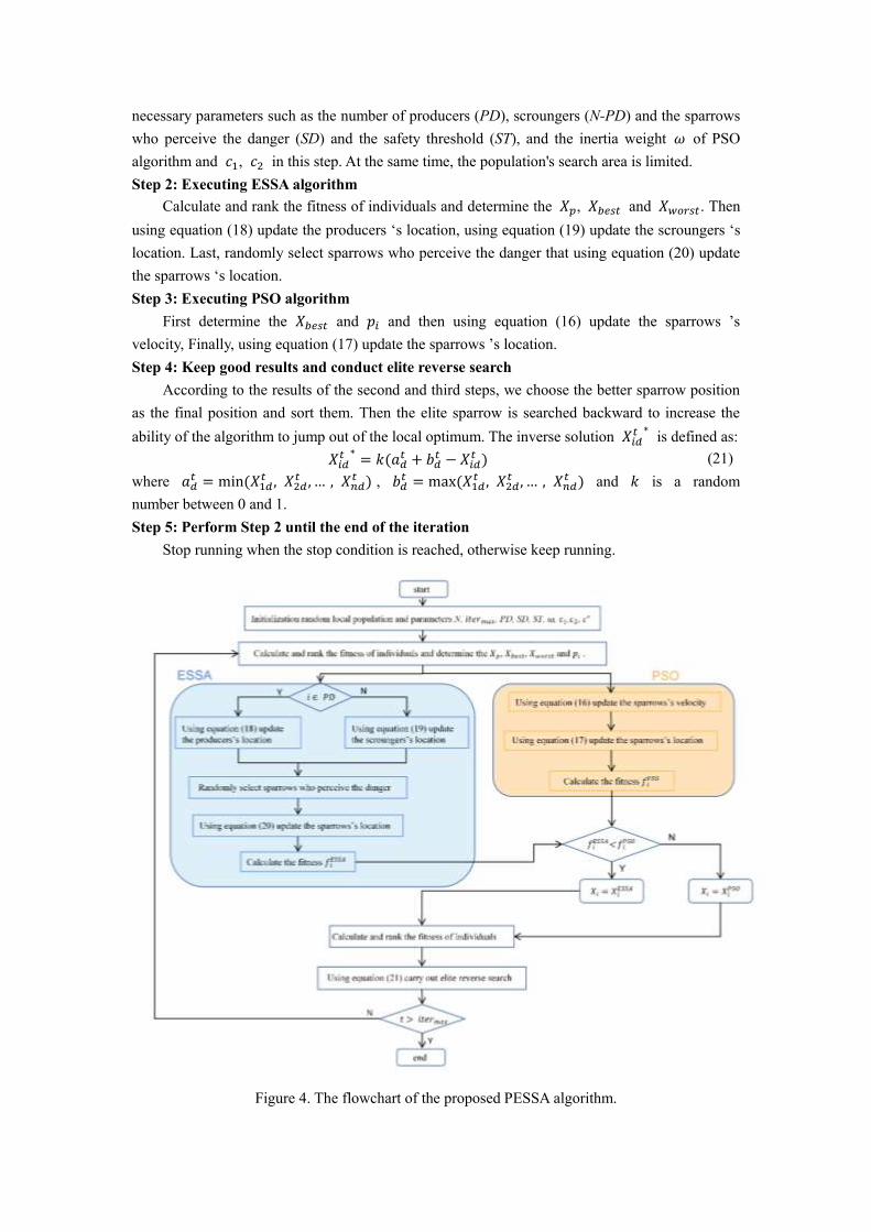
necessary parameters such as the number of producers (PD), scroungers (N-PD) and the sparrows who perceive the danger (SD) and the safety threshold (ST), and the inertia weight 𝜔 of PSO algorithm and 𝑐1, 𝑐2 in this step. At the same time, the population's search area is limited. Step 2: Executing ESSA algorithm

Calculate and rank the fitness of individuals and determine the 𝑋𝑝, 𝑋𝑏𝑒𝑠𝑡 and 𝑋𝑤𝑜𝑟𝑠𝑡. Then using equation (18) update the producers ‘s location, using equation (19) update the scroungers ‘s location. Last, randomly select sparrows who perceive the danger that using equation (20) update the sparrows ‘s location. Step 3: Executing PSO algorithm

First determine the 𝑋𝑏𝑒𝑠𝑡 and 𝑝𝑖 and then using equation (16) update the sparrows ’s velocity, Finally, using equation (17) update the sparrows ’s location. Step 4: Keep good results and conduct elite reverse search

According to the results of the second and third steps, we choose the better sparrow position as the final position and sort them. Then the elite sparrow is searched backward to increase the ability of the algorithm to jump out of the local optimum. The inverse solution 𝑋𝑖𝑑𝑡 ∗ is defined as: 𝑋𝑖𝑑𝑡 ∗ = 𝑘(𝑎𝑑𝑡 + 𝑏𝑑𝑡 − 𝑋𝑖𝑑𝑡 ) (21) where 𝑎𝑑𝑡 = min (𝑋1𝑑𝑡 , 𝑋2𝑑𝑡 , … , 𝑋𝑛𝑑𝑡 ) , 𝑏𝑑𝑡 = max (𝑋1𝑑𝑡 , 𝑋2𝑑𝑡 , … , 𝑋𝑛𝑑𝑡 ) and 𝑘 is a random number between 0 and 1. Step 5: Perform Step 2 until the end of the iteration

Stop running when the stop condition is reached, otherwise keep running.

Figure 4. The flowchart of the proposed PESSA algorithm.

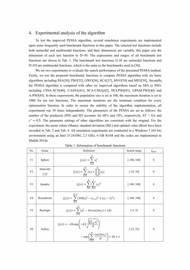
4. Experimental analysis of the algorithm

To test the improved PESSA algorithm, several simulation experiments are implemented upon some frequently used benchmark functions in this paper. The selected test functions include both unimodal and multimodal functions, and their dimensions are variable, this paper sets the dimension of each test function to D=30. The expressions and ranges of all benchmark test functions are shown in Tab. 1. The benchmark test functions f1-f4 are unimodal functions and f5-f10 are multimodal functions, which is the same as the benchmarks used in [30].

We set two experiments to evaluate the search performance of the presented PESSA method. Firstly, we use the proposed benchmark functions to compare PESSA algorithm with six basic algorithms including SSA[30], PSO[35], GWO[36], SCA[37], MVO[38] and MFO[39],. Secondly, the PESSA algorithm is compared with other six improved algorithms based on SSA or PSO, including CSSA-SCN[40], CASSA[41], SCA-CSSA[42], HCLPSO[43], GPAM-PSO[44] and A-PSO[45]. In these experiments, the population size is set at 100, the maximum iteration is set to 1000 for ten test functions. The maximum iterations are the terminate condition for every optimization function. In order to ensure the stability of the algorithm implementation, all experiments run 30 times independently. The parameters of the PESSA are set as follows: the number of the producers (PD) and SD accounts for 60% and 10%, respectively, ST = 0.6 and 𝑐∗ = 0.5. The parameter settings of other algorithms are consistent with the original. For the experiment, the mean values (Mean), standard deviation (SD.) and optimal value (Best) have been recorded in Tab. 2 and Tab. 4. All simulation experiments are conducted in a Windows 7 (64 bit) environment using an Intel i5-2410M, 2.3 GHz, 6 GB RAM and the codes are implemented in Matlab 2014a.

Table 1. Information of benchmark functions

No. Name Definition Search range 𝑓𝑚𝑖𝑛

F1 Sphere 𝑓1(𝑥) =∑𝑥𝑖2𝐷𝑖=1 [-100, 100] 0

F2 Schwefel

2.22 𝑓2(𝑥) =∑|𝑥𝑖|𝐷

𝑖=1 +∏|𝑥𝑖|𝐷𝑖=1 [-10, 10] 0

F3 Quadric 𝑓3(𝑥) =∑(∑𝑥𝑗𝑖𝑗=1 )2𝐷

𝑖=1 [-100, 100] 0

F4 Rosenbrock 𝑓4(𝑥) = ∑(100(𝑥𝑖2 − 𝑥𝑖+1)2 + (𝑥𝑖 − 1)2)𝐷−1𝑖=1 [-100, 100] 0

F5 Rastrigin 𝑓5(𝑥) =∑(𝑥𝑖2 − 10 cos(2𝜋𝑥𝑖) + 10)𝐷𝑖=1 [-5, 5] 0

F6 Ackley

𝑓6(𝑥) = −20 exp(−0.2√∑ 𝑥𝑖2𝐷𝑖=2𝐷 )− exp(∑cos(2𝜋𝑥𝑖)𝐷𝐷

𝑖=1 ) + 20 + 𝑒

[-32, 32] 0

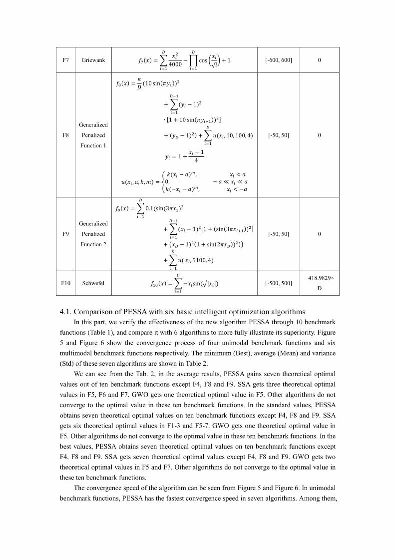
F7 Griewank 𝑓7(𝑥) =∑ 𝑥𝑖24000 −∏cos (𝑥𝑖√𝑖) + 1𝐷𝑖=1

𝐷𝑖=1 [-600, 600] 0

F8

Generalized

Penalized

Function 1

𝑓8(𝑥) = 𝜋𝐷 (10 sin(𝜋𝑦1))2+∑(𝑦𝑖 − 1)2𝐷−1𝑖=1∙ [1 + 10 sin(𝜋𝑦𝑖+1))2]+ (𝑦𝐷 − 1)2) +∑𝑢(𝑥𝑖 , 10, 100, 4)𝐷

𝑖=1

𝑦𝑖 = 1 + 𝑥𝑖 + 14 𝑢(𝑥𝑖 , 𝑎, 𝑘,𝑚) = { 𝑘(𝑥𝑖 − 𝑎)𝑚 , 𝑥𝑖 < 𝑎0, − 𝑎 ≪ 𝑥𝑖 ≪ 𝑎𝑘(−𝑥𝑖 − 𝑎)𝑚 , 𝑥𝑖 < −𝑎

[-50, 50] 0

F9

Generalized

Penalized

Function 2

𝑓9(𝑥) =∑0.1(sin (3𝜋𝑥1)2𝐷𝑖=1 +∑(𝑥𝑖 − 1)2[1 + (sin(3𝜋𝑥𝑖+1))2]𝐷−1

𝑖=1+ (𝑥𝐷 − 1)2(1 + sin(2𝜋𝑥𝐷))2))+∑𝑢(𝐷𝑖=1 𝑥𝑖 , 5100, 4)

[-50, 50] 0

F10 Schwefel 𝑓10(𝑥) =∑−𝑥𝑖sin (√|𝑥𝑖|)𝐷𝑖=1 [-500, 500]

−418.9829×

D

4.1. Comparison of PESSA with six basic intelligent optimization algorithms

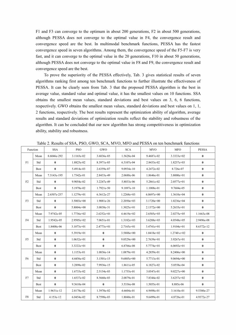
In this part, we verify the effectiveness of the new algorithm PESSA through 10 benchmark functions (Table 1), and compare it with 6 algorithms to more fully illustrate its superiority. Figure 5 and Figure 6 show the convergence process of four unimodal benchmark functions and six multimodal benchmark functions respectively. The minimum (Best), average (Mean) and variance (Std) of these seven algorithms are shown in Table 2.

We can see from the Tab. 2, in the average results, PESSA gains seven theoretical optimal values out of ten benchmark functions except F4, F8 and F9. SSA gets three theoretical optimal values in F5, F6 and F7. GWO gets one theoretical optimal value in F5. Other algorithms do not converge to the optimal value in these ten benchmark functions. In the standard values, PESSA obtains seven theoretical optimal values on ten benchmark functions except F4, F8 and F9. SSA gets six theoretical optimal values in F1-3 and F5-7. GWO gets one theoretical optimal value in F5. Other algorithms do not converge to the optimal value in these ten benchmark functions. In the best values, PESSA obtains seven theoretical optimal values on ten benchmark functions except F4, F8 and F9. SSA gets seven theoretical optimal values except F4, F8 and F9. GWO gets two theoretical optimal values in F5 and F7. Other algorithms do not converge to the optimal value in these ten benchmark functions.

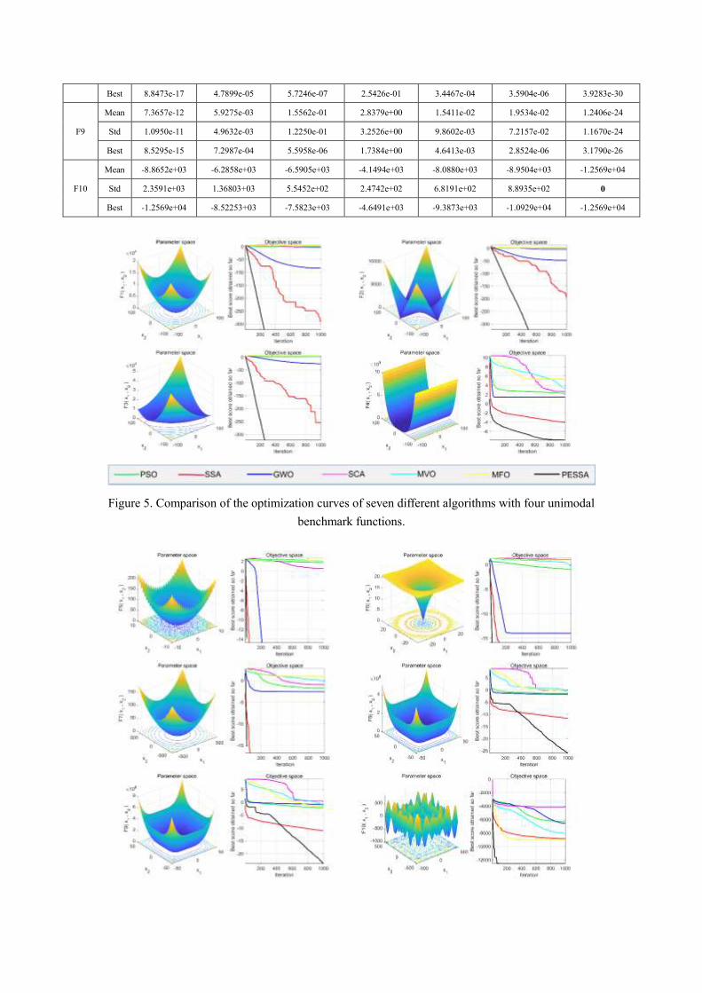
The convergence speed of the algorithm can be seen from Figure 5 and Figure 6. In unimodal benchmark functions, PESSA has the fastest convergence speed in seven algorithms. Among them,

F1 and F3 can converge to the optimum in about 200 generations, F2 in about 500 generations, although PESSA does not converge to the optimal value in F4, the convergence result and convergence speed are the best. In multimodal benchmark functions, PESSA has the fastest convergence speed in seven algorithms. Among them, the convergence speed of the F5-F7 is very fast, and it can converge to the optimal value in the 20 generations, F10 in about 50 generations, although PESSA does not converge to the optimal value in F8 and F9, the convergence result and convergence speed are the best.

To prove the superiority of the PESSA effectively, Tab. 3 gives statistical results of seven algorithms ranking first among ten benchmark functions to further illustrate the effectiveness of PESSA. It can be clearly seen from Tab. 3 that the proposed PESSA algorithm is the best in average value, standard value and optimal value, it has the smallest values on 10 functions. SSA obtains the smallest mean values, standard deviations and best values on 3, 6, 6 functions, respectively. GWO obtains the smallest mean values, standard deviations and best values on 1, 1, 2 functions, respectively. The best results represent the optimization ability of algorithm, average results and standard deviations of optimization results reflect the stability and robustness of the algorithm. It can be concluded that our new algorithm has strong competitiveness in optimization ability, stability and robustness.

Table 2. Results of SSA, PSO, GWO, SCA, MVO, MFO and PESSA on ten benchmark functions

Function SSA PSO GWO SCA MVO MFO PESSA

F1

Mean 8.6046e-292 3.1165e-02 3.6836e-85 1.5628e-04 9.4687e-02 3.3333e+02 0

Std 0 1.8825e-02 8.3971e-85 6.3107e-04 2.8433e-02 1.8257e+03 0

Best 0 5.4914e-03 2.6359e-87 9.0934e-10 4.2472e-02 8.726e-07 0

F2

Mean 7.3143e-195 1.7342e-01 2.8433e-49 2.0688e-06 1.8646e-01 3.8000e+01 0

Std 0 9.9054e-02 3.2247e-49 5.8033e-06 5.2861e-02 2.0577e+01 0

Best 0 5.1978e-02 1.7921e-50 9.1897e-10 1.1008e-01 9.7604e-05 0

F3

Mean 2.6507e-257 1.1279e+01 6.3612e-27 1.2268e+03 6.8697e+00 1.3610e+04 0

Std 0 3.5003e+00 1.9081e-26 2.2050e+03 3.1720e+00 1.0236e+04 0

Best 0 5.8004e+00 3.0838e-31 1.3025e+01 2.1372e+00 5.2635e+01 0

F4

Mean 7.9742e-05 1.7736e+02 2.6252e+01 4.4619e+02 2.6585e+03 2.0275e+05 1.1663e-08

Std 1.9542e-05 2.9505e+02 7.0651e-01 1.3182e+03 3.6288e+03 4.0548e+05 2.9496e-08

Best 1.8408e-06 3.1073e+01 2.4773e+01 2.7165e+01 3.4741e+01 1.9104e+01 8.6372e-12

F5

Mean 0 5.3919e+01 0 3.5888e+00 1.0418e+02 1.2740 e+02 0

Std 0 1.0632e+01 0 9.0529e+00 2.7639e+01 3.9267e+01 0

Best 0 3.3222e+01 0 6.8766e-08 5.7774e+01 6.0692e+01 0

F6

Mean 0 1.1153e-01 1.0836e-14 1.0879e+01 4.2859e-01 8.2406e+00 0

Std 0 4.4456e-02 3.1501e-15 9.6805e+00 5.7713e-01 9.0694e+00 0

Best 0 3.2898e-02 7.9936e-15 1.8611e-05 6.1827e-02 5.0558e-04 0

F7

Mean 0 1.6733e-02 2.5154e-03 1.1755e-01 3.0547e-01 9.0227e+00 0

Std 0 1.6537e-02 8.5660e-03 2.0879e-01 7.8344e-02 3.6257e+02 0

Best 0 9.3610e-04 0 3.5336e-08 1.5055e-01 8.885e-06 0

F8

Mean 1.9631e-12 2.8178e-02 1.3970e-02 4.6604e-01 6.9498e-01 3.1610e-01 9.5380e-27

Std 4.153e-12 6.0454e-02 8.7598e-03 1.8040e-01 9.6499e-01 4.8726e-01 4.9372e-27

Best 8.8473e-17 4.7899e-05 5.7246e-07 2.5426e-01 3.4467e-04 3.5904e-06 3.9283e-30

F9

Mean 7.3657e-12 5.9275e-03 1.5562e-01 2.8379e+00 1.5411e-02 1.9534e-02 1.2406e-24

Std 1.0950e-11 4.9632e-03 1.2250e-01 3.2526e+00 9.8602e-03 7.2157e-02 1.1670e-24

Best 8.5295e-15 7.2987e-04 5.5958e-06 1.7384e+00 4.6413e-03 2.8524e-06 3.1790e-26

F10

Mean -8.8652e+03 -6.2858e+03 -6.5905e+03 -4.1494e+03 -8.0880e+03 -8.9504e+03 -1.2569e+04

Std 2.3591e+03 1.36803+03 5.5452e+02 2.4742e+02 6.8191e+02 8.8935e+02 0

Best -1.2569e+04 -8.52253+03 -7.5823e+03 -4.6491e+03 -9.3873e+03 -1.0929e+04 -1.2569e+04

Figure 5. Comparison of the optimization curves of seven different algorithms with four unimodal benchmark functions.

Figure 6. Comparison of the optimization curves of seven different algorithms with six multimodal benchmark functions.

Table 3. Statistical results of ten different benchmark functions. SSA PSO GWO SCA MVO MFO PESSA

Mean 3 0 1 0 0 0 10

Std 6 0 1 0 0 0 10

Best 6 0 2 0 0 0 10

4.2. Comparison of PESSA with six related improved algorithms

In this section, to prove the superiority of the PESSA effectively, the proposed PESSA algorithm is compared with six improved algorithms based on SSA or PSO algorithm, including the CSSA-SCN, CASSA, SCA-CSSA, HCLPSO, GPAM-PSO and A-PSO. The experimental results of ten benchmark functions are given as shown in Tab. 4.

We can see from the Tab. 4, in the average results, PESSA gains seven theoretical optimal values out of ten benchmark functions except F4, F8 and F9, but it can find solutions which are very close to the optimal values (the deviation is less than e-10) on these two functions F8 and F9. CSSA-SCN gets five theoretical optimal values on F1-F3, F5 and F7, and can find solution which is very close to the optimal value on F6. A-PSO gets two theoretical optimal values in F5 and F7, GPAM-PSO gets one theoretical optimal value on F7, and can find solutions which are very close to the optimal values on these three functions F1, F3 and F6. A-PSO gets two theoretical optimal values on F5 and F7, and can find solutions which are very close to the optimal values on these four functions F1, F2, F3 and F6. Other algorithms do not converge to the optimal value in these ten benchmark functions. SCA-CSSA can find solutions which are very close to the optimal values on F6. HCLPSO can find solutions which are very close to the optimal values on these six functions F1, F2, F6, F7, F8 and F9. In the standard values, PESSA obtains seven theoretical optimal values on ten benchmark functions except F4, F8 and F9, but it can find solutions which are very close to the optimal values on these two functions F8 and F9. CSSA-SCN gets five theoretical optimal values on F1-F3, F5 and F7, and can find solution which is very close to the optimal value on F6. GPAM-PSO gets one theoretical optimal value on F7, and can find solutions which are very close to the optimal values on these two functions F1 and F3. A-PSO gets five theoretical optimal values on F1-F3, F5 and F7, and can find solution which is very close to the optimal value on F6. Other algorithms do not converge to the optimal value in these ten benchmark functions. SCA-CSSA can find solutions which are very close to the optimal values on F6. HCLPSO can find solutions which are very close to the optimal values on these six functions F1, F2, F6, F7, F8 and F9. In the best values, PESSA obtains seven theoretical optimal values on ten benchmark functions except F4, F8 and F9, but it can find solutions which are very close to the optimal values on these three functions F4, F8 and F9. CSSA-SCN gets six theoretical optimal values on F1-F3, F5, F7 and F10, and can find solutions which are very close to the optimal values on these three functions F6, F8 and F9. CASSA gets five theoretical optimal value on F1, F3, F5-F7, and can find solutions which are very close to the optimal values on F8. SCA-CSSA gets five theoretical optimal value on F1-F3, F5 and F7, and can find solutions which are very close to

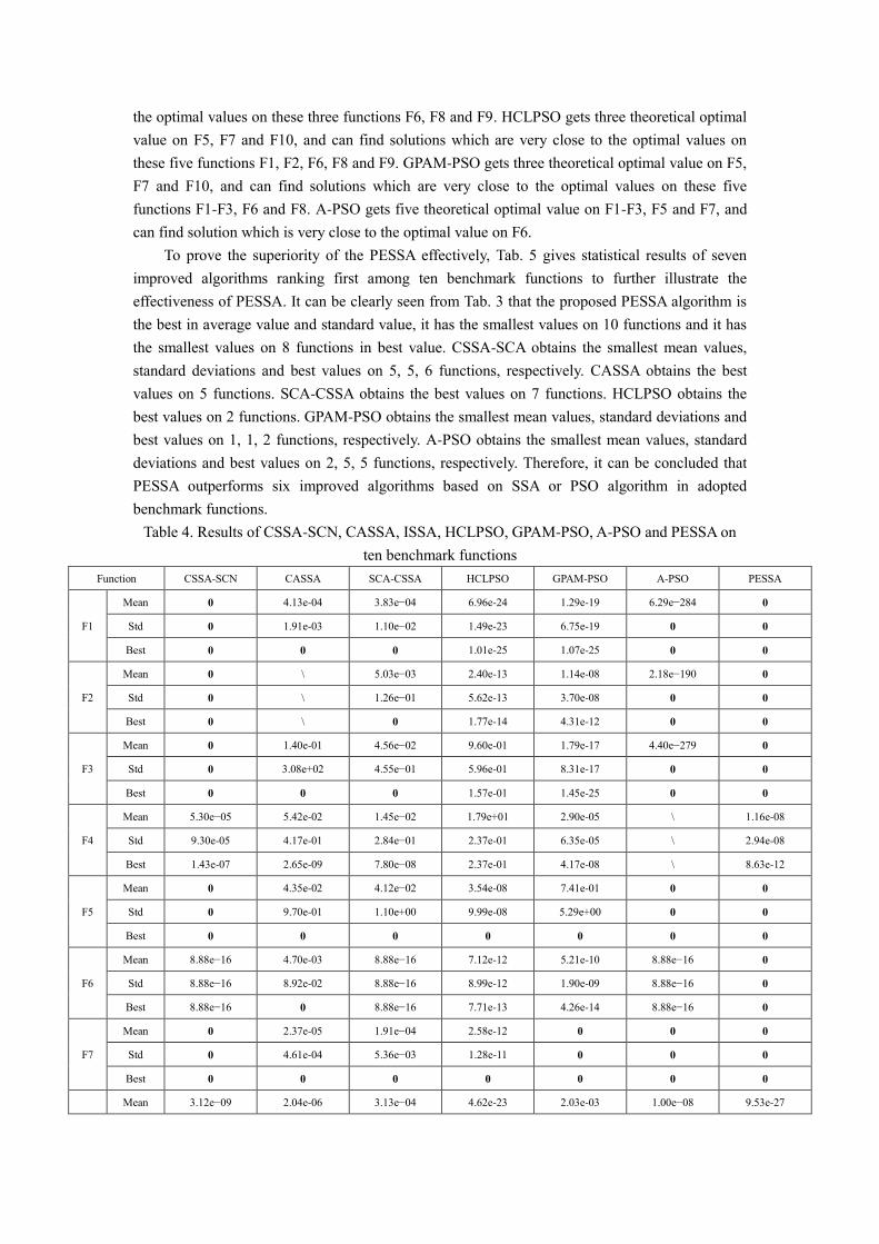
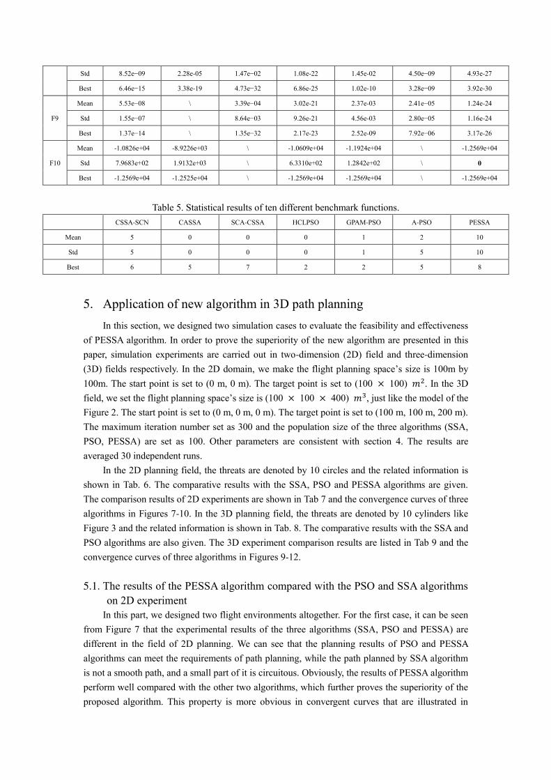
the optimal values on these three functions F6, F8 and F9. HCLPSO gets three theoretical optimal value on F5, F7 and F10, and can find solutions which are very close to the optimal values on these five functions F1, F2, F6, F8 and F9. GPAM-PSO gets three theoretical optimal value on F5, F7 and F10, and can find solutions which are very close to the optimal values on these five functions F1-F3, F6 and F8. A-PSO gets five theoretical optimal value on F1-F3, F5 and F7, and can find solution which is very close to the optimal value on F6. To prove the superiority of the PESSA effectively, Tab. 5 gives statistical results of seven improved algorithms ranking first among ten benchmark functions to further illustrate the effectiveness of PESSA. It can be clearly seen from Tab. 3 that the proposed PESSA algorithm is the best in average value and standard value, it has the smallest values on 10 functions and it has the smallest values on 8 functions in best value. CSSA-SCA obtains the smallest mean values, standard deviations and best values on 5, 5, 6 functions, respectively. CASSA obtains the best values on 5 functions. SCA-CSSA obtains the best values on 7 functions. HCLPSO obtains the best values on 2 functions. GPAM-PSO obtains the smallest mean values, standard deviations and best values on 1, 1, 2 functions, respectively. A-PSO obtains the smallest mean values, standard deviations and best values on 2, 5, 5 functions, respectively. Therefore, it can be concluded that PESSA outperforms six improved algorithms based on SSA or PSO algorithm in adopted benchmark functions.

Table 4. Results of CSSA-SCN, CASSA, ISSA, HCLPSO, GPAM-PSO, A-PSO and PESSA on ten benchmark functions

Function CSSA-SCN CASSA SCA-CSSA HCLPSO GPAM-PSO A-PSO PESSA

F1

Mean 0 4.13e-04 3.83e−04 6.96e-24 1.29e-19 6.29e−284 0

Std 0 1.91e-03 1.10e−02 1.49e-23 6.75e-19 0 0

Best 0 0 0 1.01e-25 1.07e-25 0 0

F2

Mean 0 \ 5.03e−03 2.40e-13 1.14e-08 2.18e−190 0

Std 0 \ 1.26e−01 5.62e-13 3.70e-08 0 0

Best 0 \ 0 1.77e-14 4.31e-12 0 0

F3

Mean 0 1.40e-01 4.56e−02 9.60e-01 1.79e-17 4.40e−279 0

Std 0 3.08e+02 4.55e−01 5.96e-01 8.31e-17 0 0

Best 0 0 0 1.57e-01 1.45e-25 0 0

F4

Mean 5.30e−05 5.42e-02 1.45e−02 1.79e+01 2.90e-05 \ 1.16e-08

Std 9.30e-05 4.17e-01 2.84e−01 2.37e-01 6.35e-05 \ 2.94e-08

Best 1.43e-07 2.65e-09 7.80e−08 2.37e-01 4.17e-08 \ 8.63e-12

F5

Mean 0 4.35e-02 4.12e−02 3.54e-08 7.41e-01 0 0

Std 0 9.70e-01 1.10e+00 9.99e-08 5.29e+00 0 0

Best 0 0 0 0 0 0 0

F6

Mean 8.88e−16 4.70e-03 8.88e−16 7.12e-12 5.21e-10 8.88e−16 0

Std 8.88e−16 8.92e-02 8.88e−16 8.99e-12 1.90e-09 8.88e−16 0

Best 8.88e−16 0 8.88e−16 7.71e-13 4.26e-14 8.88e−16 0

F7

Mean 0 2.37e-05 1.91e−04 2.58e-12 0 0 0

Std 0 4.61e-04 5.36e−03 1.28e-11 0 0 0

Best 0 0 0 0 0 0 0

F8

Mean 3.12e−09 2.04e-06 3.13e−04 4.62e-23 2.03e-03 1.00e−08 9.53e-27

Std 8.52e−09 2.28e-05 1.47e−02 1.08e-22 1.45e-02 4.50e−09 4.93e-27

Best 6.46e−15 3.38e-19 4.73e−32 6.86e-25 1.02e-10 3.28e−09 3.92e-30

F9

Mean 5.53e−08 \ 3.39e−04 3.02e-21 2.37e-03 2.41e−05 1.24e-24

Std 1.55e−07 \ 8.64e−03 9.26e-21 4.56e-03 2.80e−05 1.16e-24

Best 1.37e−14 \ 1.35e−32 2.17e-23 2.52e-09 7.92e−06 3.17e-26

F10

Mean -1.0826e+04 -8.9226e+03 \ -1.0609e+04 -1.1924e+04 \ -1.2569e+04

Std 7.9683e+02 1.9132e+03 \ 6.3310e+02 1.2842e+02 \ 0

Best -1.2569e+04 -1.2525e+04 \ -1.2569e+04 -1.2569e+04 \ -1.2569e+04

Table 5. Statistical results of ten different benchmark functions. CSSA-SCN CASSA SCA-CSSA HCLPSO GPAM-PSO A-PSO PESSA

Mean 5 0 0 0 1 2 10

Std 5 0 0 0 1 5 10

Best 6 5 7 2 2 5 8

5. Application of new algorithm in 3D path planning

In this section, we designed two simulation cases to evaluate the feasibility and effectiveness of PESSA algorithm. In order to prove the superiority of the new algorithm are presented in this paper, simulation experiments are carried out in two-dimension (2D) field and three-dimension (3D) fields respectively. In the 2D domain, we make the flight planning space’s size is 100m by 100m. The start point is set to (0 m, 0 m). The target point is set to (100 × 100) 𝑚2. In the 3D field, we set the flight planning space’s size is (100 × 100 × 400) 𝑚3, just like the model of the Figure 2. The start point is set to (0 m, 0 m, 0 m). The target point is set to (100 m, 100 m, 200 m). The maximum iteration number set as 300 and the population size of the three algorithms (SSA, PSO, PESSA) are set as 100. Other parameters are consistent with section 4. The results are averaged 30 independent runs.

In the 2D planning field, the threats are denoted by 10 circles and the related information is shown in Tab. 6. The comparative results with the SSA, PSO and PESSA algorithms are given. The comparison results of 2D experiments are shown in Tab 7 and the convergence curves of three algorithms in Figures 7-10. In the 3D planning field, the threats are denoted by 10 cylinders like Figure 3 and the related information is shown in Tab. 8. The comparative results with the SSA and PSO algorithms are also given. The 3D experiment comparison results are listed in Tab 9 and the convergence curves of three algorithms in Figures 9-12.

5.1. The results of the PESSA algorithm compared with the PSO and SSA algorithms on 2D experiment

In this part, we designed two flight environments altogether. For the first case, it can be seen from Figure 7 that the experimental results of the three algorithms (SSA, PSO and PESSA) are different in the field of 2D planning. We can see that the planning results of PSO and PESSA algorithms can meet the requirements of path planning, while the path planned by SSA algorithm is not a smooth path, and a small part of it is circuitous. Obviously, the results of PESSA algorithm perform well compared with the other two algorithms, which further proves the superiority of the proposed algorithm. This property is more obvious in convergent curves that are illustrated in

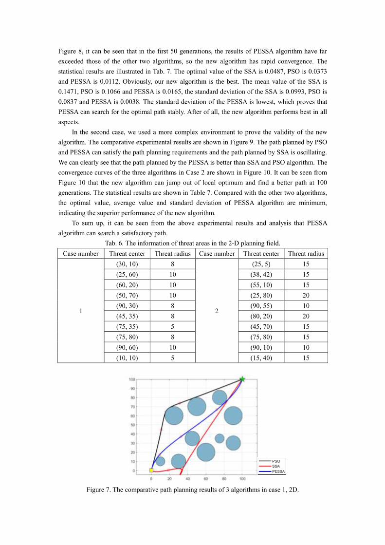
Figure 8, it can be seen that in the first 50 generations, the results of PESSA algorithm have far exceeded those of the other two algorithms, so the new algorithm has rapid convergence. The statistical results are illustrated in Tab. 7. The optimal value of the SSA is 0.0487, PSO is 0.0373 and PESSA is 0.0112. Obviously, our new algorithm is the best. The mean value of the SSA is 0.1471, PSO is 0.1066 and PESSA is 0.0165, the standard deviation of the SSA is 0.0993, PSO is 0.0837 and PESSA is 0.0038. The standard deviation of the PESSA is lowest, which proves that PESSA can search for the optimal path stably. After of all, the new algorithm performs best in all aspects.

In the second case, we used a more complex environment to prove the validity of the new algorithm. The comparative experimental results are shown in Figure 9. The path planned by PSO and PESSA can satisfy the path planning requirements and the path planned by SSA is oscillating. We can clearly see that the path planned by the PESSA is better than SSA and PSO algorithm. The convergence curves of the three algorithms in Case 2 are shown in Figure 10. It can be seen from Figure 10 that the new algorithm can jump out of local optimum and find a better path at 100 generations. The statistical results are shown in Table 7. Compared with the other two algorithms, the optimal value, average value and standard deviation of PESSA algorithm are minimum, indicating the superior performance of the new algorithm.

To sum up, it can be seen from the above experimental results and analysis that PESSA algorithm can search a satisfactory path.

Tab. 6. The information of threat areas in the 2-D planning field. Case number Threat center Threat radius Case number Threat center Threat radius

1

(30, 10) 8

2

(25, 5) 15

(25, 60) 10 (38, 42) 15

(60, 20) 10 (55, 10) 15

(50, 70) 10 (25, 80) 20

(90, 30) 8 (90, 55) 10

(45, 35) 8 (80, 20) 20

(75, 35) 5 (45, 70) 15

(75, 80) 8 (75, 80) 15

(90, 60) 10 (90, 10) 10

(10, 10) 5 (15, 40) 15

Figure 7. The comparative path planning results of 3 algorithms in case 1, 2D.

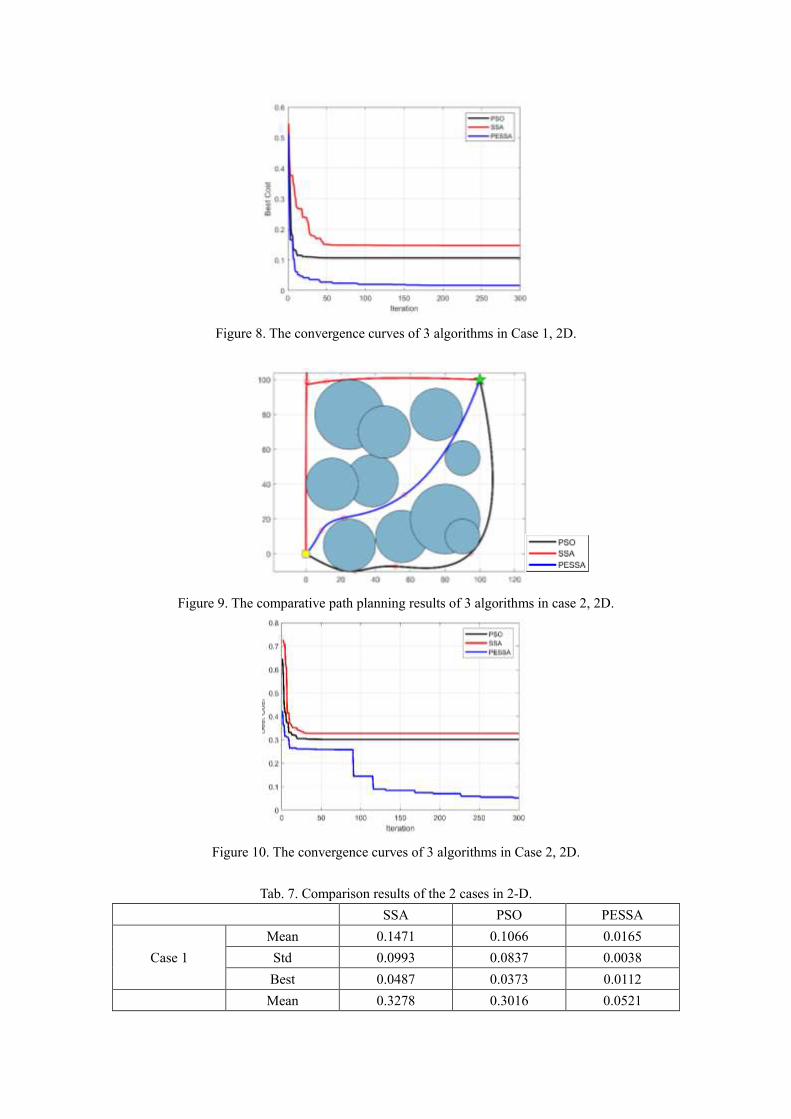
Figure 8. The convergence curves of 3 algorithms in Case 1, 2D.

Figure 9. The comparative path planning results of 3 algorithms in case 2, 2D.

Figure 10. The convergence curves of 3 algorithms in Case 2, 2D.

Tab. 7. Comparison results of the 2 cases in 2-D. SSA PSO PESSA

Case 1

Mean 0.1471 0.1066 0.0165

Std 0.0993 0.0837 0.0038

Best 0.0487 0.0373 0.0112

Case 2Mean 0.3278 0.3016 0.0521

Std 0.2837 0.1727 0.0048

Best 0.1382 0.0837 0.0382

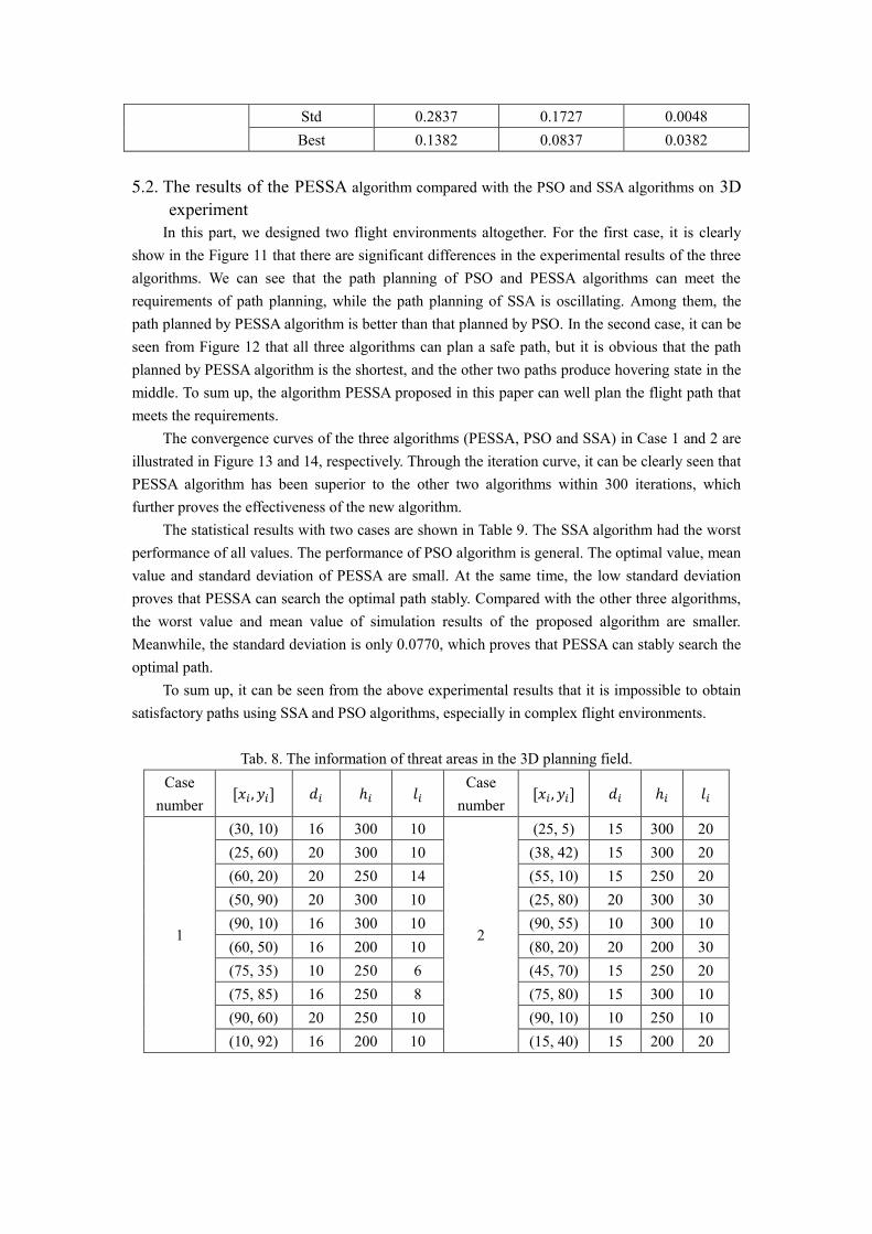
5.2. The results of the PESSA algorithm compared with the PSO and SSA algorithms on 3D experiment

In this part, we designed two flight environments altogether. For the first case, it is clearly show in the Figure 11 that there are significant differences in the experimental results of the three algorithms. We can see that the path planning of PSO and PESSA algorithms can meet the requirements of path planning, while the path planning of SSA is oscillating. Among them, the path planned by PESSA algorithm is better than that planned by PSO. In the second case, it can be seen from Figure 12 that all three algorithms can plan a safe path, but it is obvious that the path planned by PESSA algorithm is the shortest, and the other two paths produce hovering state in the middle. To sum up, the algorithm PESSA proposed in this paper can well plan the flight path that meets the requirements.

The convergence curves of the three algorithms (PESSA, PSO and SSA) in Case 1 and 2 are illustrated in Figure 13 and 14, respectively. Through the iteration curve, it can be clearly seen that PESSA algorithm has been superior to the other two algorithms within 300 iterations, which further proves the effectiveness of the new algorithm.

The statistical results with two cases are shown in Table 9. The SSA algorithm had the worst performance of all values. The performance of PSO algorithm is general. The optimal value, mean value and standard deviation of PESSA are small. At the same time, the low standard deviation proves that PESSA can search the optimal path stably. Compared with the other three algorithms, the worst value and mean value of simulation results of the proposed algorithm are smaller. Meanwhile, the standard deviation is only 0.0770, which proves that PESSA can stably search the optimal path.

To sum up, it can be seen from the above experimental results that it is impossible to obtain satisfactory paths using SSA and PSO algorithms, especially in complex flight environments.

Tab. 8. The information of threat areas in the 3D planning field. Case

number [𝑥𝑖 , 𝑦𝑖] 𝑑𝑖 ℎ𝑖 𝑙𝑖 Case

number [𝑥𝑖 , 𝑦𝑖] 𝑑𝑖 ℎ𝑖 𝑙𝑖

1

(30, 10) 16 300 10

2

(25, 5) 15 300 20

(25, 60) 20 300 10 (38, 42) 15 300 20

(60, 20) 20 250 14 (55, 10) 15 250 20

(50, 90) 20 300 10 (25, 80) 20 300 30

(90, 10) 16 300 10 (90, 55) 10 300 10

(60, 50) 16 200 10 (80, 20) 20 200 30

(75, 35) 10 250 6 (45, 70) 15 250 20

(75, 85) 16 250 8 (75, 80) 15 300 10

(90, 60) 20 250 10 (90, 10) 10 250 10

(10, 92) 16 200 10 (15, 40) 15 200 20

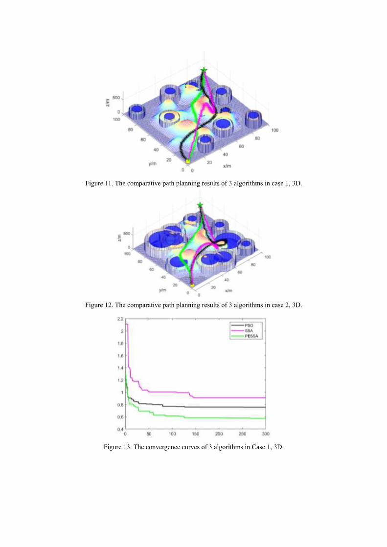
Figure 11. The comparative path planning results of 3 algorithms in case 1, 3D.

Figure 12. The comparative path planning results of 3 algorithms in case 2, 3D.

Figure 13. The convergence curves of 3 algorithms in Case 1, 3D.

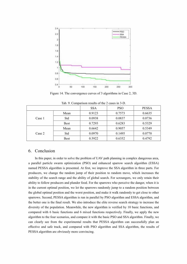
Figure 14. The convergence curves of 3 algorithms in Case 2, 3D.

Tab. 9. Comparison results of the 2 cases in 3-D. SSA PSO PESSA

Case 1

Mean 0.9123 0.7573 0.6635

Std 0.0938 0.0837 0.0736

Best 0.7293 0.6283 0.5329

Case 2

Mean 0.6642 0.9057 0.5349

Std 0.0970 0.1495 0.0770

Best 0.5922 0.6352 0.4792

6. Conclusion

In this paper, in order to solve the problem of UAV path planning in complex dangerous area, a parallel particle swarm optimization (PSO) and enhanced sparrow search algorithm (ESSA) named PESSA algorithm is presented. At first, we improve the SSA algorithm in three parts. For producers, we change the random jump of their position to random move, which increases the stability of the search range and the ability of global search. For scroungers, we only retain their ability to follow producers and plunder food. For the sparrows who perceive the danger, when it is in the current optimal position, we let the sparrows randomly jump to a random position between the global optimal position and the worst position, and make it walk randomly to get close to other sparrows. Second, PESSA algorithm is run in parallel by PSO algorithm and ESSA algorithm, and the better one is the final result. We also introduce the elite reverse search strategy to increase the diversity of the population. Meanwhile, the new algorithm is verified by 10 basic functions, and compared with 6 basic functions and 6 mixed functions respectively. Finally, we apply the new algorithm to the four scenarios, and compare it with the basic PSO and SSA algorithm. Finally, we can clearly see from the experimental results that PESSA algorithm can successfully plan an effective and safe track, and compared with PSO algorithm and SSA algorithm, the results of PESSA algorithm are obviously more convincing.

References

1. Sun, C.; Liu, Y.C.; Dai, R.; Grymin, D. Two approaches for path planning of unmanned aerial

vehicles with avoidance zones. J. Guid. Control. Dyn. 2017, 40, 2076–2083,

doi:10.2514/1.G002314.

2. Zhang, Z.; Li, J.; Wang, J. Sequential convex programming for nonlinear optimal control

problems in UAV path planning. Aerosp. Sci. Technol. 2018, 76, 280–290,

doi:10.1016/j.ast.2018.01.040.

3. Zhao, Y.; Yan, L.; Chen, Y.; Dai, J.; Liu, Y. Robust and efficient trajectory replanning based

on guiding path for quadrotor fast autonomous flight. Remote Sens. 2021, 13, 1–26,

doi:10.3390/rs13050972.

4. Tang, G.; Tang, C.; Zhou, H.; Claramunt, C.; Men, S. R-dfs: A coverage path planning

approach based on region optimal decomposition. Remote Sens. 2021, 13,

doi:10.3390/rs13081525.

5. Mangeruga, M.; Casavola, A.; Pupo, F.; Bruno, F. An underwater pathfinding algorithm for

optimised planning of survey dives. Remote Sens. 2020, 12, 1–17, doi:10.3390/rs12233974.

6. Koch, T.; Körner, M.; Fraundorfer, F. Automatic and semantically-aware 3D UAV flight

planning for image-based 3D reconstruction. Remote Sens. 2019, 11, 1–29,

doi:10.3390/rs11131550.

7. Pehlivanoglu, Y.V. A new vibrational genetic algorithm enhanced with a Voronoi diagram for

path planning of autonomous UAV. Aerosp. Sci. Technol. 2012, 16, 47–55,

doi:10.1016/j.ast.2011.02.006.

8. Melchior, P.; Orsoni, B.; Lavialle, O.; Poty, A.; Oustaloup, A. Consideration of obstacle danger

level in path planning using A * and Fast-Marching optimisation: Comparative study. Signal

Processing 2003, 83, 2387–2396.

9. Koenig, S.; Likhachev, M. Fast replanning for navigation in unknown terrain. IEEE Trans.

Robot. 2005, 21, 354–363, doi:10.1109/TRO.2004.838026.

10. Shier, D.R. On algorithms for finding the k shortest paths in a network. Networks 1979, 9, 195–214, doi:10.1002/net.3230090303.

11. Fu, Y.; Ding Prof., M.; Zhou Prof., C.; Hu, H. Route planning for unmanned aerial vehicle

(UAV) on the sea using hybrid differential evolution and quantum-behaved particle swarm

optimization. IEEE Trans. Syst. Man, Cybern. Syst. 2013, 43, 1451–1465,

doi:10.1109/TSMC.2013.2248146.

12. Szczerba, R.J.; Galkowski, P.; Glickstein, I.S.; Ternullo, N. Robust algorithm for real-time

route planning. IEEE Trans. Aerosp. Electron. Syst. 2000, 36, 869–878, doi:10.1109/7.869506.

13. Niu, H.; Lu, Y.; Savvaris, A.; Tsourdos, A. An energy-efficient path planning algorithm for

unmanned surface vehicles. Ocean Eng. 2018, 161, 308–321,

doi:10.1016/j.oceaneng.2018.01.025.

14. Zhang, X.; Duan, H. An improved constrained differential evolution algorithm for unmanned

aerial vehicle global route planning. Appl. Soft Comput. J. 2015, 26, 270–284,

doi:10.1016/j.asoc.2014.09.046.

15. Zhang, D.; Duan, H. Social-class pigeon-inspired optimization and time stamp segmentation

for multi-UAV cooperative path planning. Neurocomputing 2018, 313, 229–246,

doi:10.1016/j.neucom.2018.06.032.

16. Yu, X.; Li, C.; Zhou, J.F. A constrained differential evolution algorithm to solve UAV path

planning in disaster scenarios. Knowledge-Based Syst. 2020, 204,

doi:10.1016/j.knosys.2020.106209.

17. Liu, Y.; Zhang, X.; Guan, X.; Delahaye, D. Adaptive sensitivity decision based path planning

algorithm for unmanned aerial vehicle with improved particle swarm optimization. Aerosp. Sci.

Technol. 2016, 58, 92–102, doi:10.1016/j.ast.2016.08.017.

18. Jiang, X.; Lin, Z.; He, T.; Ma, X.; Ma, S.; Li, S. Optimal Path Finding with Beetle Antennae

Search Algorithm by Using Ant Colony Optimization Initialization and Different Searching

Strategies. IEEE Access 2020, 8, 15459–15471, doi:10.1109/ACCESS.2020.2965579.

19. Song, P.C.; Pan, J.S.; Chu, S.C. A parallel compact cuckoo search algorithm for

three-dimensional path planning. Appl. Soft Comput. J. 2020, 94, 106443,

doi:10.1016/j.asoc.2020.106443.

20. Phung, M.D.; Ha, Q.P. Safety-enhanced UAV path planning with spherical vector-based

particle swarm optimization. Appl. Soft Comput. 2021, 107, 107376,

doi:10.1016/j.asoc.2021.107376.

21. Dewangan, R.K.; Shukla, A.; Godfrey, W.W. Three dimensional path planning using Grey

wolf optimizer for UAVs. Appl. Intell. 2019, 49, 2201–2217, doi:10.1007/s10489-018-1384-y.

22. Huang, C.; Fei, J.; Deng, W. A Novel Route Planning Method of Fixed-Wing Unmanned

Aerial Vehicle Based on Improved QPSO. IEEE Access 2020, 8, 65071–65084,

doi:10.1109/ACCESS.2020.2984236.

23. Sánchez-García, J.; Reina, D.G.; Toral, S.L. A distributed PSO-based exploration algorithm for

a UAV network assisting a disaster scenario. Futur. Gener. Comput. Syst. 2019, 90, 129–148,

doi:10.1016/j.future.2018.07.048.

24. Thangaraj, R.; Pant, M.; Abraham, A.; Bouvry, P. Particle swarm optimization: Hybridization

perspectives and experimental illustrations. Appl. Math. Comput. 2011, 217, 5208–5226,

doi:10.1016/j.amc.2010.12.053.

25. Rodriguez, F.J.; García-Martinez, C.; Lozano, M. Hybrid metaheuristics based on evolutionary

algorithms and simulated annealing: Taxonomy, comparison, and synergy test. IEEE Trans.

Evol. Comput. 2012, 16, 787–800, doi:10.1109/TEVC.2012.2182773.

26. Fodorean, D.; Idoumghar, L.; Brevilliers, M.; Minciunescu, P.; Irimia, C. Hybrid Differential

Evolution Algorithm Employed for the Optimum Design of a High-Speed PMSM Used for EV

Propulsion. IEEE Trans. Ind. Electron. 2017, 64, 9824–9833, doi:10.1109/TIE.2017.2701788.

27. Das, P.K.; Behera, H.S.; Panigrahi, B.K. A hybridization of an improved particle swarm

optimization and gravitational search algorithm for multi-robot path planning. Swarm Evol.

Comput. 2016, 28, 14–28, doi:10.1016/j.swevo.2015.10.011.

28. Qu, C.; Gai, W.; Zhang, J.; Zhong, M. A novel hybrid grey wolf optimizer algorithm for

unmanned aerial vehicle (UAV) path planning. Knowledge-Based Syst. 2020, 194, 105530,

doi:10.1016/j.knosys.2020.105530.

29. Wang, X.; Zhao, H.; Han, T.; Zhou, H.; Li, C. A grey wolf optimizer using Gaussian estimation

of distribution and its application in the multi-UAV multi-target urban tracking problem. Appl.

Soft Comput. J. 2019, 78, 240–260, doi:10.1016/j.asoc.2019.02.037.

30. Xue, J.; Shen, B. A novel swarm intelligence optimization approach: sparrow search algorithm.

Syst. Sci. Control Eng. 2020, 8, 22–34, doi:10.1080/21642583.2019.1708830.

31. Roberge, V.; Tarbouchi, M.; Labonte, G. Comparison of parallel genetic algorithm and particle

swarm optimization for real-time UAV path planning. IEEE Trans. Ind. Informatics 2013, 9,

132–141, doi:10.1109/TII.2012.2198665.

32. Sariff, N.; Buniyamin, N. An Overview of Autonomous Mobile Robot Path Planning

Algorithms. 2006, 183–188.

33. Sun, Z.; Wu, J.; Yang, J.; Huang, Y.; Li, C.; Li, D. Path Planning for GEO-UAV Bistatic SAR

Using Constrained Adaptive Multiobjective Differential Evolution. IEEE Trans. Geosci.

Remote Sens. 2016, 54, 6444–6457, doi:10.1109/TGRS.2016.2585184.

34. Nikolos, I.K.; Valavanis, K.P.; Tsourveloudis, N.C.; Kostaras, A.N. Evolutionary Algorithm

Based Offline/Online Path Planner for UAV Navigation. IEEE Trans. Syst. Man, Cybern. Part

B Cybern. 2003, 33, 898–912, doi:10.1109/TSMCB.2002.804370.

35. Okwu, M.O.; Tartibu, L.K. Particle Swarm Optimisation. Stud. Comput. Intell. 2021, 927, 5–13,

doi:10.1007/978-3-030-61111-8_2.

36. Mirjalili, S.; Mirjalili, S.M.; Lewis, A. Grey Wolf Optimizer. Adv. Eng. Softw. 2014, 69, 46–61,

doi:10.1016/j.advengsoft.2013.12.007.

37. Mirjalili, S. SCA: A Sine Cosine Algorithm for solving optimization problems.

Knowledge-Based Syst. 2016, 96, 120–133, doi:10.1016/j.knosys.2015.12.022.

38. Mirjalili, S.; Mirjalili, S.M.; Hatamlou, A. Multi-Verse Optimizer : a nature-inspired algorithm

for global optimization. Neural Comput. Appl. 2016, 495–513,

doi:10.1007/s00521-015-1870-7.

39. Mirjalili, S. Moth-flame optimization algorithm: A novel nature-inspired heuristic paradigm.

Knowledge-Based Syst. 2015, 89, 228–249, doi:10.1016/j.knosys.2015.07.006.

40. Zhang, C.; Ding, S. A stochastic configuration network based on chaotic sparrow search

algorithm. Knowledge-Based Syst. 2021, 220, 106924, doi:10.1016/j.knosys.2021.106924.

41. Liu, G.; Shu, C.; Liang, Z.; Peng, B.; Cheng, L. A modified sparrow search algorithm with

application in 3d route planning for uav. Sensors (Switzerland) 2021, 21, 1–23,

doi:10.3390/s21041224.

42. Zhang, J.; Xia, K.; He, Z.; Yin, Z.; Wang, S. Semi-Supervised Ensemble Classifier with

Improved Sparrow Search Algorithm and Its Application in Pulmonary Nodule Detection.

Math. Probl. Eng. 2021, 2021, doi:10.1155/2021/6622935.

43. Lynn, N.; Suganthan, P.N. Heterogeneous comprehensive learning particle swarm optimization

with enhanced exploration and exploitation. Swarm Evol. Comput. 2015, 24, 11–24,

doi:10.1016/j.swevo.2015.05.002.

44. Cui, Q.; Li, Q.; Li, G.; Li, Z.; Han, X.; Lee, H.P.; Liang, Y.; Wang, B.; Jiang, J.; Wu, C.

Globally-optimal prediction-based adaptive mutation particle swarm optimization. Inf. Sci. (Ny).

2017, 418–419, 186–217, doi:10.1016/j.ins.2017.07.038.

45. Chen, K.; Zhou, F.; Wang, Y.; Yin, L. An ameliorated particle swarm optimizer for solving

numerical optimization problems. Appl. Soft Comput. J. 2018, 73, 482–496,

doi:10.1016/j.asoc.2018.09.007.

Data availability

The datasets generated and/or analysed during the current study are not publicly available due the need for graduation thesis but are available from the corresponding author on reasonable request.