f ¨ ur Mathematik in den Naturwissenschaften Leipzig A Parabolic Free Boundary Problem with Bernoulli Type Condition on the Free Boundary by John Andersson, and Georg Weiss Preprint no.: 119 2006

Welcome message from author
This document is posted to help you gain knowledge. Please leave a comment to let me know what you think about it! Share it to your friends and learn new things together.
Transcript
Max-Plan k-Institutfur Mathematik
in den Naturwissenschaften
Leipzig
A Parabolic Free Boundary Problem with
Bernoulli Type Condition on the Free Boundary
by
John Andersson, and Georg Weiss
Preprint no.: 119 2006

A PARABOLIC FREE BOUNDARY PROBLEM WITH
BERNOULLI TYPE CONDITION ON THE FREE BOUNDARY
JOHN ANDERSSON AND GEORG S. WEISS
Abstract. Consider the parabolic free boundary problem
∆u − ∂tu = 0 in u > 0 , |∇u| = 1 on ∂u > 0 .
For a realistic class of solutions, containing for example all limits of the singular
perturbation problem
∆uε − ∂tuε = βε(uε) as ε → 0,
we prove that one-sided flatness of the free boundary implies regularity.
In particular, we show that the topological free boundary ∂u > 0 can be
decomposed into an open regular set (relative to ∂u > 0) which is locally a
surface with Holder-continuous space normal, and a closed singular set.
Our result extends the main theorem in the paper by H.W. Alt-L.A. Caffarelli
(1981) to more general solutions as well as the time-dependent case. Our proof
uses methods developed in H.W. Alt-L.A. Caffarelli (1981), however we replace
the core of that paper, which relies on non-positive mean curvature at singular
points, by an argument based on scaling discrepancies, which promises to be
applicable to more general free boundary or free discontinuity problems.
1. Introduction
The parabolic free boundary problem
(1.1) ∆u− ∂tu = 0 in u > 0 , |∇u| = 1 on ∂u > 0
has originally been derived as singular limit from a model for the propagation
of equidiffusional premixed flames with high activation energy ([3]); here u =
λ(Tc − T ) , Tc is the flame temperature, which is assumed to be constant, T is
the temperature outside the flame and λ is a normalization factor.
Let us shortly summarize the mathematical results directly relevant in this context,
beginning with the limit problem (1.1): in the brilliant paper [1], H.W. Alt and L.A.
2000 Mathematics Subject Classification. Primary 35R35, Secondary 35K55.
Key words and phrases. Free boundary, Bernoulli type, parabolic, regularity, flatness improve-
ment.
J. Andersson has been partially supported by a fellowship of the Max Planck Society. G.S.
Weiss has been partially supported by the Grant-in-Aid 15740100/18740086 of the Japanese Min-
istry of Education, Culture, Sports, Science and Technology and partially supported by a fellow-
ship of the Max Planck Society. Both authors thank the Max Planck Institute for Mathematics
in the Sciences for the hospitality during their stay in Leipzig.
1
2 J. ANDERSSON AND G.S. WEISS
Caffarelli proved via minimization of the energy∫
(|∇u|2 + χu>0) – here χu>0denotes the characteristic function of the set u > 0 – existence of a stationary so-
lution of (1.1) in the sense of distributions. They also derived regularity of the free
boundary ∂u > 0 up to a set of vanishing n− 1-dimensional Hausdorff measure.
By [12] existence of singular minimizers implies the existence of singular minimizing
cones. L.A. Caffarelli-D. Jerison-C. Kenig showed that singular minimizing cones
do not exist in dimension 3 ([6]). Moreover it is known that singular minimizing
cones exist for n ≥ 7 ([8]). Non-minimizing singular cones appear already for n = 3
(see [1, example 2.7]). Moreover it is known, that solutions of the Dirichlet problem
in two space dimensions are not unique (see [1, example 2.6]).
For the time-dependent (1.1), both “trivial non-uniqueness” (the positive solution
of the heat equation is always another solution of (1.1)) and “non-trivial unique-
ness” (see [10]) occur. Even for flawless initial data, classical solutions of (1.1)
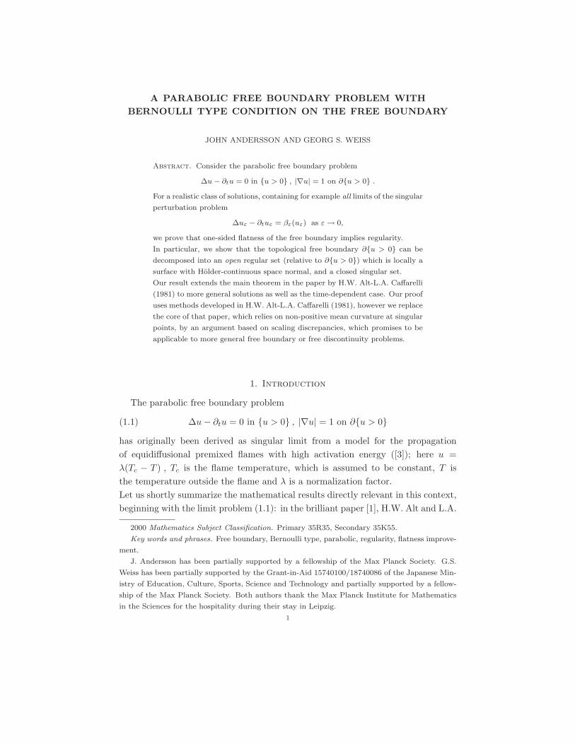
develop singularities after a finite time span; consider e.g. the example of two
colliding traveling waves
(1.2)u(t, x) = χx+t>1(exp(x+ t− 1) − 1)
+ χ−x+t>1(exp(−x+ t− 1) − 1) for t ∈ [0, 1)
(see Figure 1).
u > 0 u > 0
u = 0
x = 0 x = 1x = −1
t = 1
t = 0
Figure 1. Colliding traveling waves
There are several approaches concerning the construction of a solution of the time-
dependent problem, all of which are based in some form on the convergence of the
solution uε of the reaction-diffusion equation
(1.3) ∆uε − ∂tuε = βε(uε)
to (1.1) as ε→ 0; here βε(z) = 1εβ( z
ε ) , β ∈ C10 ([0, 1]) , β > 0 in (0, 1) and
∫
β = 12 .
L.A. Caffarelli and J.L. Vazquez proved in [7] uniform estimates for (1.3) and a
convergence result: for initial data u0 that are strictly mean concave in the interior
A PARABOLIC FREE BOUNDARY PROBLEM 3
of their support, a sequence of ε-solutions converges to a solution of (1.1) in the
sense of distributions.
Let us also mention several results on the corresponding two-phase problem, which
are relevant as solutions of the one-phase problem are automatically solutions of
the corresponding two-phase problem. In [5] and [4], L.A. Caffarelli, C. Lederman
and N. Wolanski prove convergence to a barrier solution in the case that the limit
function satisfies u = 0 = ∅ .Then, there is the convergence to a solution in the sense of domain variations [11]
which seems to contain more information than the barrier solutions in [5] and [4].
For more general two-phase problems see [13]. Domain variation solutions play an
important rule in this paper and will be discussed in more detail in Section 3.
Here let it suffice to say that domain variation solutions are pairs (u, χ) where the
order parameter χ shares many properties with the characteristic function χu>0but does not necessarily coincide with it. By [11], all limits of the singular pertur-
bation problem (1.3) are domain variation solutions, so all results in the present
paper hold for all limits of (1.3).
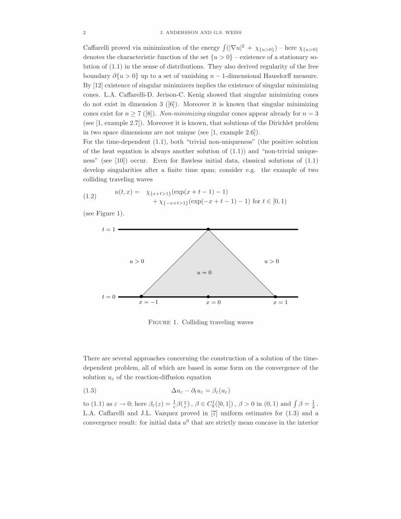
Our main result Theorem 8.4 states – leaving out inessential assumptions – that
if (0, ρ2) is a point on the topological free boundary and if the set χ > 0 is flat
enough, i.e.
χ(x, t) = 0 when (x, t) ∈ Qρ and xn ≥ σρ,
for some σ ≤ σ0 (see Figure 2), then the free boundary Qρ/4∩∂u > 0 is a surface
with Holder-continuous space normal.
As a consequence we obtain that the regular set is open relative to ∂u > 0
xn > σ
χ > 0χ = 0
(x, t) = (0, 1)
Figure 2. One-sided flatness in the case ρ = 1
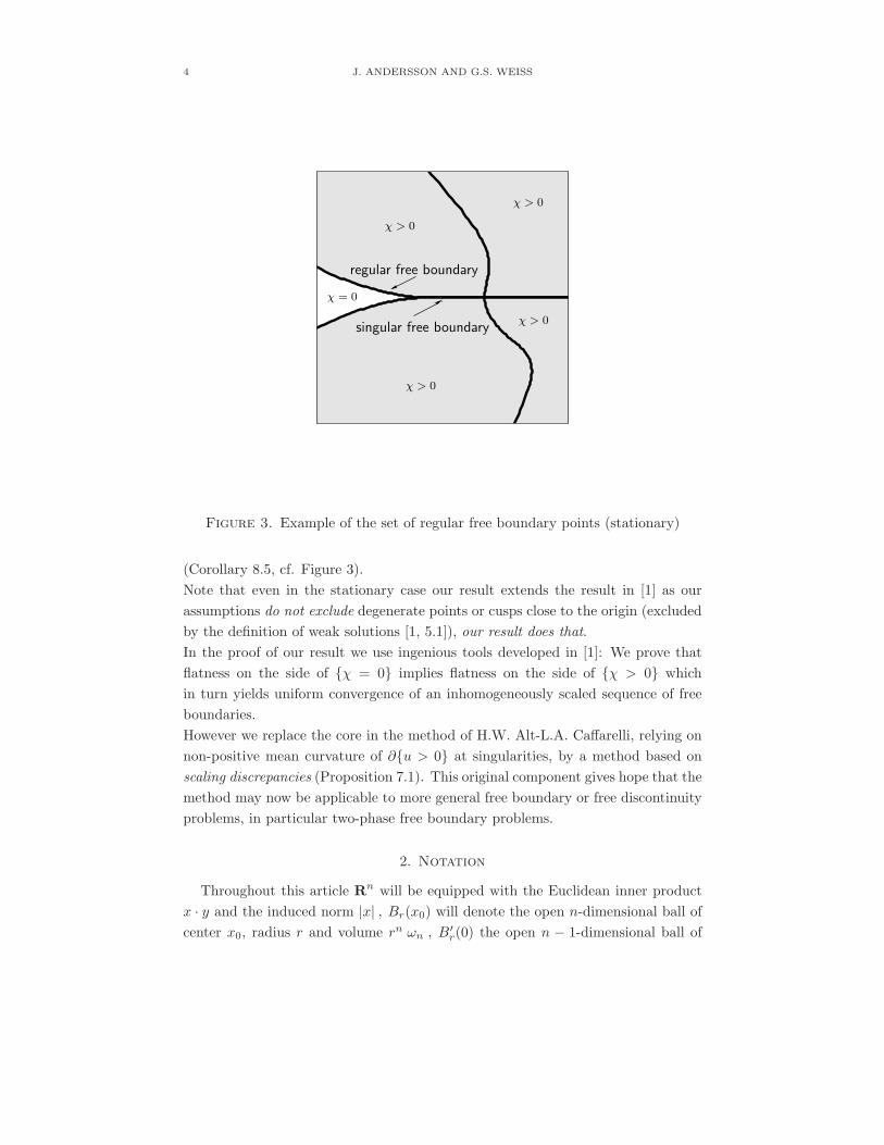
4 J. ANDERSSON AND G.S. WEISS
χ = 0
χ > 0
χ > 0singular free boundary
χ > 0
χ > 0
regular free boundary
Figure 3. Example of the set of regular free boundary points (stationary)
(Corollary 8.5, cf. Figure 3).
Note that even in the stationary case our result extends the result in [1] as our
assumptions do not exclude degenerate points or cusps close to the origin (excluded
by the definition of weak solutions [1, 5.1]), our result does that.
In the proof of our result we use ingenious tools developed in [1]: We prove that
flatness on the side of χ = 0 implies flatness on the side of χ > 0 which
in turn yields uniform convergence of an inhomogeneously scaled sequence of free
boundaries.
However we replace the core in the method of H.W. Alt-L.A. Caffarelli, relying on
non-positive mean curvature of ∂u > 0 at singularities, by a method based on
scaling discrepancies (Proposition 7.1). This original component gives hope that the
method may now be applicable to more general free boundary or free discontinuity
problems, in particular two-phase free boundary problems.
2. Notation
Throughout this article Rn will be equipped with the Euclidean inner product
x · y and the induced norm |x| , Br(x0) will denote the open n-dimensional ball of
center x0, radius r and volume rn ωn , B′r(0) the open n − 1-dimensional ball of
A PARABOLIC FREE BOUNDARY PROBLEM 5
center 0 and radius r, and ei the i-th unit vector in Rn. We define Qr(x0, t0) :=
Br(x0)×(t0−r2, t0+r2) to be the cylinder of radius r and height 2r2, Q−r (x0, t0) :=
Br(x0) × (t0 − r2, t0) its “negative part” and T−r (t0) := Rn × (t0 − 4r2, t0 − r2)
the horizontal layer from t0 − 4r2 to t0 − r2. Let us also introduce the parabolic
distance pardist((t, x), A) := inf(s,y)∈A
√
|x− y|2 + |t− s|. Considering a function
φ ∈ H1,2loc (Rn;Rn) we denote by div φ :=
∑ni=1 ∂iφi the space divergence and by
Dφ :=
∂1φ1 . . . ∂nφ1
. . .
∂1φn . . . ∂nφn
the matrix of the spatial partial derivatives.
Given a set A ⊂ Rn , we denote its interior by A and its characteristic function
by χA . In the text we use the n-dimensional Lebesgue-measure Ln and the m-
dimensional Hausdorff measure Hm. When considering a given set A ⊂ Rn, let
∂MA := x ∈ Rn : lim supr→0
Ln(Br(x) ∩A)
Ln(Br)> 0 and lim sup
r→0
Ln(Br(x) −A)
Ln(Br)> 0
be the measure-theoretic boundary of A, let ∂∗A := x ∈ Rn : there is ν(x) ∈∂B1(0) such that r−n
∫
Br(x)|χA − χy:(y−x)·ν(x)<0| → 0 as r → 0 (by [14, Corol-
lary 5.6.8] ∂∗A coincides Hn−1-a.e. with the reduced boundary of a set of finite
perimeter defined in [14, Definition 5.5.1]), and let ν : ∂∗A → ∂B1(0) denote this
measure theoretic outward normal to ∂A. We shall often use abbreviations for in-
verse images like u > 0 := x ∈ Ω : u(x) > 0 , xn > 0 := x ∈ Rn : xn >
0 , s = t := (s, y) ∈ Rn+1 : s = t etc. as well as A(t) := A ∩ s = t for
a set A ⊂ Rn+1, and occasionally we employ the decomposition x = (x′, xn) of a
vector x ∈ Rn as well as the corresponding decompositions of the gradient and the
Laplace operator,
∇u = (∇′u, ∂nu) and ∆u = ∆′u + ∂nnu .
Finally, Cβ,µ := Hµ,β denotes the parabolic Holder-space defined in [9].
3. Notion of solution and Preliminaries
In this section we gather some results from [11]. As degenerate points are un-
avoidable in the parabolic problem (see the introduction of [11] for examples), an
extension of the weak solutions in [1] does not seem to be the right choice. Instead
we use the solutions of [11, Definition 6.1], which are, roughly speaking, solutions in
the sense of domain variations. The advantage is that the class of solutions defined
in [11, Definition 6.1] is closed under the blow-up process. Moreover, all limits of
the singular perturbation problem discussed in [7] are domain variation solutions
and satisfy [11, Definition 6.1] (see [11, Section 6]). Let us recall the definition of
solutions and the monotonicity formula used therein:
6 J. ANDERSSON AND G.S. WEISS
Theorem 3.1 (Monotonicity Formula, cf. [11, Theorem 5.2]). Let (x0, t0) ∈ Rn ×(0,∞) , T−
r (t0) = Rn × (t0 − 4r2, t0 − r2) , 0 < ρ < σ <√
t02 and
G(x0,t0)(x, t) = 4π(t0 − t) |4π(t0 − t)|−n2−1
exp
(
−|x− x0|24(t0 − t)
)
.
Then
Ψ(x0,t0)(r) = r−2∫
T−r (t0)
(
|∇u|2 + χ)
G(x0,t0) − 12 r
−2∫
T−r (t0)
1t0−t u
2 G(x0,t0)
satisfies the monotonicity formula
Ψ(x0,t0)(σ) − Ψ(x0,t0)(ρ)
≥∫ σ
ρ
r−1−2
∫
T−r (t0)
1
t0 − t
(
∇u · (x− x0) − 2(t0 − t)∂tu − u
)2
G(x0,t0) dr ≥ 0 .
Definition 3.2 (cf. [11, Definition 6.1]). We call (u, χ) a solution in Ω0 := Rn ×(0,∞) (in which case we set τ := 0) or Ω1 := Rn × (−∞,∞) (in which case we set
τ := 1), if:
1) u ∈ C1, 1
2
loc (Ωτ )∩C2(Ωτ ∩u > 0)∩H1,2loc (Ωτ ) and χ ∈ L1((−τR,R);BV (BR(0)))
for each R ∈ (0,∞) . For each R ∈ (0,∞) and δ ∈ (0, 1) there exists C1 < ∞ such
that for Qr(x0, t0) ⊂ Ωτ ∩QR(0)∫
Qr(x0,t0)
|∇χ| ≤ C1 rn+1,
∫
Qr(x0,t0)
|∂tu|2 ≤ C1 rn, and
∫
Br(x0)×(t0+S1r2,t0+S2r2)
|∂t(|∇u|2 + χ) ∗ φrδ| ≤ C1
√
S2 − S1 rn
for 0 < S1 < S2 < ∞; here the mollifier (φδ)δ∈(0,1) should be non-negative and
satisfy φδ(·) = 1δnφ( ·
δ ), φ ∈ C0,10 (Rn) ,
∫
φ = 1 and supp φ ⊂ B1(0) .
Moreover, χ ∈ 0, 1 a.e. in Ωτ and χu>0 ≤ χ a.e. in Ωτ .
2) The solution u satisfies the monotonicity formula Theorem 3.1 (in the case of
τ = 1 for (x0, t0) ∈ Rn+1 and σ ∈ (0,∞)).
3) 0 =
∫ ∞
−∞
∫
Rn
[−2∂tu∇u · ξ + (|∇u|2 + χ) div ξ − 2∇uDξ∇u]
for every ξ ∈ C0,10 (Ωτ ;Rn) .
4) The solution u is non-negative.
5) The solution u attains the initial data u0 ∈ C0,10 (Rn) in L2
loc(Rn) in the case
that τ = 0 .
6) For each κ > 0 there is δ > 0 such that Qr(x0, t0) ⊂ Ωτ and ‖u(x0+rx,t0+r2t)r −
θ|xn|‖C0(Q1(0)) < δ imply θ < 1 + κ .
A PARABOLIC FREE BOUNDARY PROBLEM 7
7) For δ ∈ (0, 1) , ψδ ∈ C0,10 (|y|2 + s2 < δ2) , ur(y, s) := u(t0+r2s,x0+ry)
r and
χr(y, s) := χ(x0 + ry, t0 + r2s) the following holds:
a)
∫
Qρ(x1,t1)
|(∇χr · x + 2t∂tχr) ∗ ψδ|
≤ C(δ, Z, T, S, ρ)
(
Ψ(x0,t0)(r
√
−t1 + δ + ρ2
2) − Ψ(x0,t0)(r
√
−t1 − δ − ρ2
2)
)
for −S ≤ t1 ≤ −T < 0 , δ + ρ2 ≤ T2 , |x1| ≤ Z and, in the case of τ = 0 , t0 −
2r2(−t1 + ρ2 + δ) > 0 .
b)
∫
Qρ(t1,x1)
|(∇χr · ξ) ∗ ψδ| ≤ C(δ)
∫
Q√δ+ρ(t1,x1)
|∇ur · ξ|
for ξ ∈ ∂B1(0) , t1 < 0 and, in the case of τ = 0 , t0 − r2(−t1 + (ρ+√δ)2) > 0 .
c)
∫ t2
t1
∂t((|∇ur|2 +χr)∗φδ)(t, x0) ≤∫ t2
t1
∫
R
2∂tur(t, z)∇ur(t, z) ·∇φδ(x0− z)dz
for −∞ < t1 < t2 <∞ and, in the case of τ = 0 , t0 + r2t1 > 0 .
Remark 3.3. As the function χ is defined only almost everywhere, all pointwise
equalities/inequalities involving χ should be understood as equalities/inequalities
that hold almost everywhere with respect to the Lebesgue measure.
The reader may wonder whether a solution in the sense of distributions (possibly
defined by the identity in [11, Lemma 11.3]) would not be good enough for the
purposes of this paper. It turns however out that the information yielded by the
order parameter χ in Definition 3.2 carries information that is essential in what
follows. Incidentally, χ may be different from χu>0 (see [11, Remark 4.1]).
Lemma 3.4. Let (u, χ) be a solution in the sense of Definition 3.2 and suppose that
for some (x0, t0) in the set of definition and for some sequence rm → 0,m→ ∞
urm(y, s) :=
u(x0 + rmy, t0 + rm2s)
rm→ 0 locally in yn < 0 × (−∞, 0) as m→ ∞
and
χrm(y, s) := χ(x0 + rmy, t0 + rm
2s) → 0 a.e. in yn > 0 × (−∞, 0) as m→ ∞ .
Then for some δ > 0, u is caloric in Qδ(x0, t0) and satisfies
u = 0 in Q−δ (x0, t0) .
Proof. The assumptions imply by Definition 3.2 1) that
urm→ 0 a.e. in xn > 0 × (−∞, 0) as m→ ∞ .
Moreover, they imply by [11, Proposition 10.1 2)] that the density
Ψ(x0,t0)(0+) ∈ 0 ∪ Hn ,
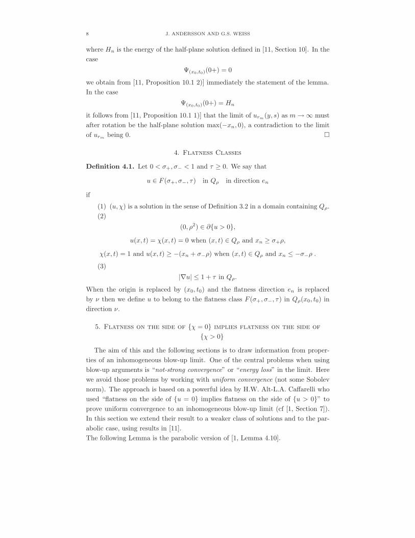
8 J. ANDERSSON AND G.S. WEISS
where Hn is the energy of the half-plane solution defined in [11, Section 10]. In the
case
Ψ(x0,t0)(0+) = 0
we obtain from [11, Proposition 10.1 2)] immediately the statement of the lemma.
In the case
Ψ(x0,t0)(0+) = Hn
it follows from [11, Proposition 10.1 1)] that the limit of urm(y, s) as m→ ∞ must
after rotation be the half-plane solution max(−xn, 0), a contradiction to the limit
of urmbeing 0.
4. Flatness Classes
Definition 4.1. Let 0 < σ+, σ− < 1 and τ ≥ 0. We say that
u ∈ F (σ+, σ−, τ) in Qρ in direction en
if
(1) (u, χ) is a solution in the sense of Definition 3.2 in a domain containing Qρ.
(2)
(0, ρ2) ∈ ∂u > 0,
u(x, t) = χ(x, t) = 0 when (x, t) ∈ Qρ and xn ≥ σ+ρ,
χ(x, t) = 1 and u(x, t) ≥ −(xn + σ−ρ) when (x, t) ∈ Qρ and xn ≤ −σ−ρ .(3)
|∇u| ≤ 1 + τ in Qρ.
When the origin is replaced by (x0, t0) and the flatness direction en is replaced
by ν then we define u to belong to the flatness class F (σ+, σ−, τ) in Qρ(x0, t0) in
direction ν.
5. Flatness on the side of χ = 0 implies flatness on the side of
χ > 0
The aim of this and the following sections is to draw information from proper-
ties of an inhomogeneous blow-up limit. One of the central problems when using
blow-up arguments is “not-strong convergence” or “energy loss” in the limit. Here
we avoid those problems by working with uniform convergence (not some Sobolev
norm). The approach is based on a powerful idea by H.W. Alt-L.A. Caffarelli who
used “flatness on the side of u = 0 implies flatness on the side of u > 0” to
prove uniform convergence to an inhomogeneous blow-up limit (cf [1, Section 7]).
In this section we extend their result to a weaker class of solutions and to the par-
abolic case, using results in [11].
The following Lemma is the parabolic version of [1, Lemma 4.10].
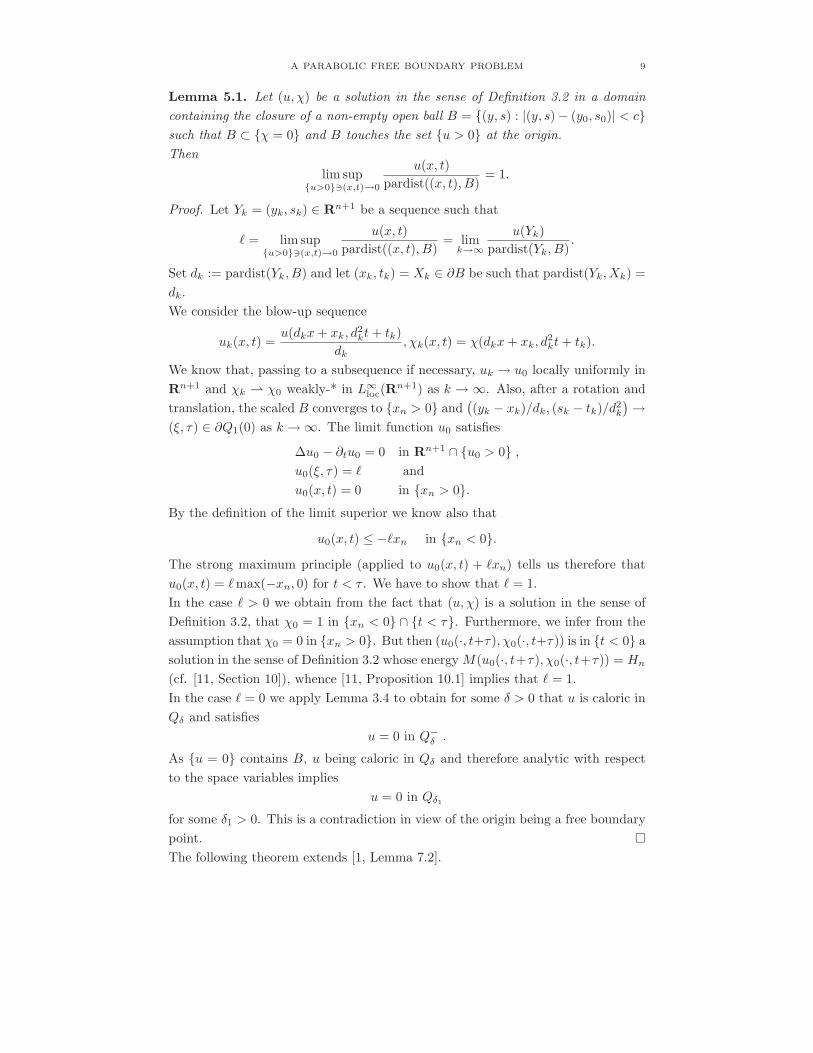
A PARABOLIC FREE BOUNDARY PROBLEM 9
Lemma 5.1. Let (u, χ) be a solution in the sense of Definition 3.2 in a domain
containing the closure of a non-empty open ball B = (y, s) : |(y, s)− (y0, s0)| < csuch that B ⊂ χ = 0 and B touches the set u > 0 at the origin.
Then
lim supu>0∋(x,t)→0
u(x, t)
pardist((x, t), B)= 1.
Proof. Let Yk = (yk, sk) ∈ Rn+1 be a sequence such that
ℓ = lim supu>0∋(x,t)→0
u(x, t)
pardist((x, t), B)= lim
k→∞
u(Yk)
pardist(Yk, B).
Set dk := pardist(Yk, B) and let (xk, tk) = Xk ∈ ∂B be such that pardist(Yk, Xk) =
dk.
We consider the blow-up sequence
uk(x, t) =u(dkx+ xk, d
2kt+ tk)
dk, χk(x, t) = χ(dkx+ xk, d
2kt+ tk).
We know that, passing to a subsequence if necessary, uk → u0 locally uniformly in
Rn+1 and χk χ0 weakly-* in L∞loc(R
n+1) as k → ∞. Also, after a rotation and
translation, the scaled B converges to xn > 0 and(
(yk − xk)/dk, (sk − tk)/d2k
)
→(ξ, τ) ∈ ∂Q1(0) as k → ∞. The limit function u0 satisfies
∆u0 − ∂tu0 = 0 in Rn+1 ∩ u0 > 0 ,u0(ξ, τ) = ℓ and
u0(x, t) = 0 in xn > 0.By the definition of the limit superior we know also that
u0(x, t) ≤ −ℓxn in xn < 0.
The strong maximum principle (applied to u0(x, t) + ℓxn) tells us therefore that
u0(x, t) = ℓmax(−xn, 0) for t < τ . We have to show that ℓ = 1.
In the case ℓ > 0 we obtain from the fact that (u, χ) is a solution in the sense of
Definition 3.2, that χ0 = 1 in xn < 0 ∩ t < τ. Furthermore, we infer from the
assumption that χ0 = 0 in xn > 0. But then (u0(·, t+τ), χ0(·, t+τ)) is in t < 0 a
solution in the sense of Definition 3.2 whose energy M(u0(·, t+τ), χ0(·, t+τ)) = Hn
(cf. [11, Section 10]), whence [11, Proposition 10.1] implies that ℓ = 1.
In the case ℓ = 0 we apply Lemma 3.4 to obtain for some δ > 0 that u is caloric in
Qδ and satisfies
u = 0 in Q−δ .
As u = 0 contains B, u being caloric in Qδ and therefore analytic with respect
to the space variables implies
u = 0 in Qδ1
for some δ1 > 0. This is a contradiction in view of the origin being a free boundary
point.
The following theorem extends [1, Lemma 7.2].
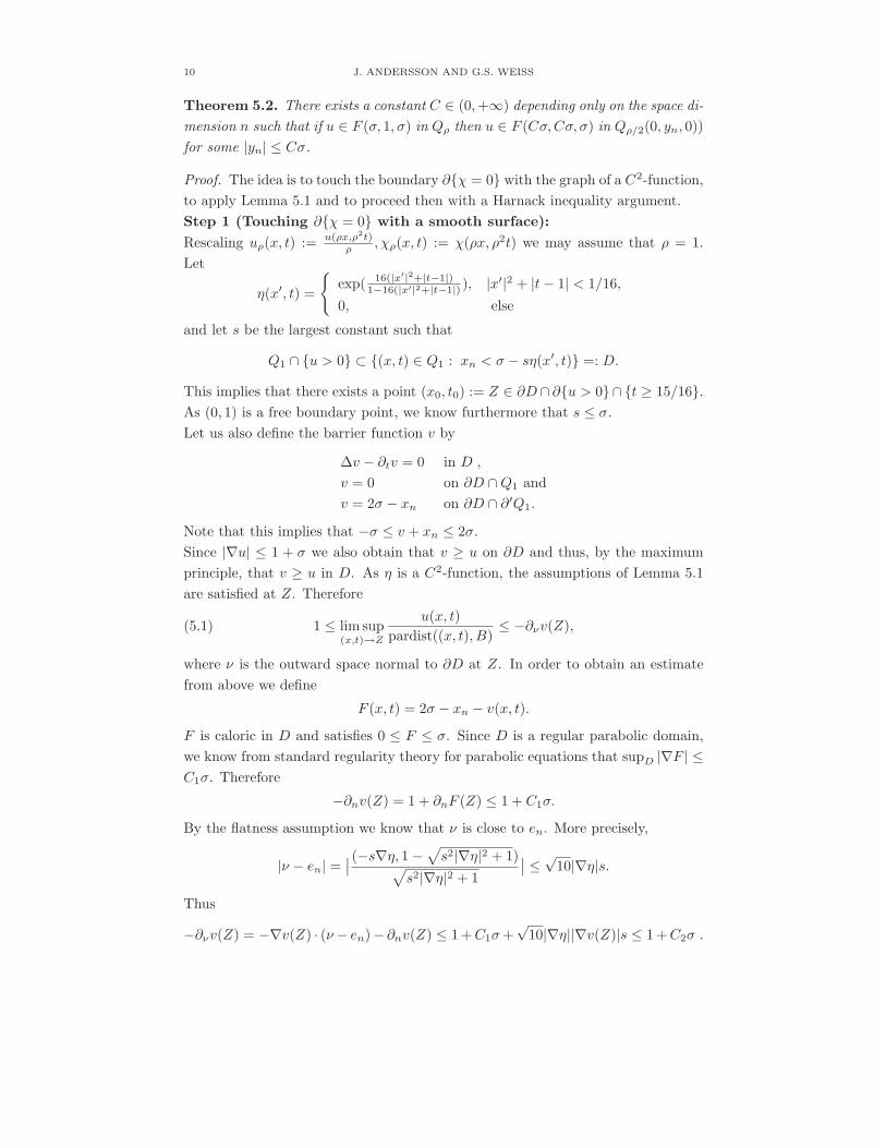
10 J. ANDERSSON AND G.S. WEISS
Theorem 5.2. There exists a constant C ∈ (0,+∞) depending only on the space di-
mension n such that if u ∈ F (σ, 1, σ) in Qρ then u ∈ F (Cσ,Cσ, σ) in Qρ/2(0, yn, 0))
for some |yn| ≤ Cσ.
Proof. The idea is to touch the boundary ∂χ = 0 with the graph of a C2-function,
to apply Lemma 5.1 and to proceed then with a Harnack inequality argument.
Step 1 (Touching ∂χ = 0 with a smooth surface):
Rescaling uρ(x, t) := u(ρx,ρ2t)ρ , χρ(x, t) := χ(ρx, ρ2t) we may assume that ρ = 1.
Let
η(x′, t) =
exp( 16(|x′|2+|t−1|)1−16(|x′|2+|t−1|) ), |x′|2 + |t− 1| < 1/16,
0, else
and let s be the largest constant such that
Q1 ∩ u > 0 ⊂ (x, t) ∈ Q1 : xn < σ − sη(x′, t) =: D.
This implies that there exists a point (x0, t0) := Z ∈ ∂D∩ ∂u > 0∩ t ≥ 15/16.As (0, 1) is a free boundary point, we know furthermore that s ≤ σ.
Let us also define the barrier function v by
∆v − ∂tv = 0 in D ,
v = 0 on ∂D ∩Q1 and
v = 2σ − xn on ∂D ∩ ∂′Q1.
Note that this implies that −σ ≤ v + xn ≤ 2σ.
Since |∇u| ≤ 1 + σ we also obtain that v ≥ u on ∂D and thus, by the maximum
principle, that v ≥ u in D. As η is a C2-function, the assumptions of Lemma 5.1
are satisfied at Z. Therefore
(5.1) 1 ≤ lim sup(x,t)→Z
u(x, t)
pardist((x, t), B)≤ −∂νv(Z),
where ν is the outward space normal to ∂D at Z. In order to obtain an estimate
from above we define
F (x, t) = 2σ − xn − v(x, t).
F is caloric in D and satisfies 0 ≤ F ≤ σ. Since D is a regular parabolic domain,
we know from standard regularity theory for parabolic equations that supD |∇F | ≤C1σ. Therefore
−∂nv(Z) = 1 + ∂nF (Z) ≤ 1 + C1σ.
By the flatness assumption we know that ν is close to en. More precisely,
|ν − en| =∣
∣
(−s∇η, 1 −√
s2|∇η|2 + 1)√
s2|∇η|2 + 1
∣
∣ ≤√
10|∇η|s.
Thus
−∂νv(Z) = −∇v(Z) · (ν − en)− ∂nv(Z) ≤ 1 +C1σ+√
10|∇η||∇v(Z)|s ≤ 1 +C2σ .
A PARABOLIC FREE BOUNDARY PROBLEM 11
From inequality (5.1) we infer that
(5.2) 1 ≤ −∂νv(Z) ≤ 1 + C2σ.
Step 2 (Harnack inequality argument):
As we know already that v is σ-close to −xn, it is sufficient to show that u is σ-close
to v on the set (x, t) : xn = −3/4, |x′| ≤ 1/2, t ≤ 3/4. Once this is done, we
may integrate u in the xn-direction to establish the lemma.
In order to prove the σ-closeness we define for ξ = (γ, τ), τ ∈ (−1, 3/4), |γ′| ≤ 1/2
and γn = −3/4 the function ωξ by
∆ωξ − ∂tωξ = 0 in D ∩ t > τωξ = −xn on B1/8(γ) × t = τωξ = 0 on the remainder of the parabolic boundary of D ∩ t > τ.
By the Hopf lemma we have
∂νωξ(Z) ≤ −α < 0
uniformly in ξ.
We would like to show that u ≥ v−C4σxn. The trick is to compare u to v−Kσωξ
on the set B1/8(γ) × t = τ and to use the information on the normal derivative
of u at Z to prove that if K is large, then u > v −Kσωξ for at least one point in
B1/8(γ) × t = τ. More precisely:
Assume that u ≤ v−Kσωξ in B1/8(γ)×t = τ. Then u ≤ v−Kσωξ in D∩t > τ.Consequently, we obtain from inequalities (5.1) and (5.2) that
1 ≤ −∂νv(Z) +Kσ∂νωξ(Z) ≤ 1 + C2σ −Kασ.
This yields a contradiction when K is large enough, say K = 2C2/α. Thus u(Xξ) >
v(Xξ) −Kσωξ(Xξ) for at least one point Xξ ∈ B1/8(γ) × t = τ.On the other hand, v− u ≥ 0. Therefore we can apply the Harnack inequality and
deduce that
(v − u)(ξ) ≤ C3 infQ1/8(ξ+(0,1/32))
(v − u) ≤ C4σ,
for every ξ ∈ (x′,−3/4, t) : |x′| < 1/2, −1 ≤ t ≤ 1/2.This implies that u(x′,−3/4, t) ≥ 3/4−C5σ in the above region. Integrating in the
en direction and using the assumption |∇u| ≤ 1 + σ yields the estimate
u ≥ −(xn + C6σ) in −3/4 ≤ xn ≤ −σ ×Q′1/2
By our initial assumption we also know that u = 0 in 3/4 ≥ xn ≥ σ ∩ Q′1/2.
Translating (u, χ) in the en direction so that the point (0, 1/4) ∈ ∂u > 0 and
using χ ≥ χu>0 of Definition 3.2 1) we obtain the statement of our theorem.
12 J. ANDERSSON AND G.S. WEISS
6. Inhomogeneous Blow-up
In this section we consider inhomogeneous scaling of the solution and the free
boundary. The following lemma is our version of [1, Lemma 7.3]
Lemma 6.1. Suppose that uk ∈ F (σk, σk, τk) in Qρk, that σk → 0 and that
τk/σ2k → 0, and define
f+k (x′, t) := suph : lim sup
r→0r−n−2
∫
Qr(ρkx′,σkρkh,ρ2kt)
χ > 0,
f−k (x′, t) := infh : lim supr→0
r−n−2
∫
Qr(ρkx′,σkρkh,ρ2kt)
χ > 0.
Then, as a subsequence k → ∞, f+k and f−k converge in L∞
loc(Q′1) to some function
f , and f is continuous in Q′1.
Proof. Rescaling as before we may assume that ρk = 1. Let
Dk := (y′, h, t) : lim supr→0
r−n−2
∫
Qr(y′,σkh,t)
χ > 0 .
We may assume – passing if necessary to a subsequence – that Dk converges with
respect to the usual (not the parabolic) Hausdorff distance as k → ∞. Let us define
f(x′, t) := lim sup(y′,s)→(x′,t),k→∞
f+k (y′, s),
where we take the limit superior with respect to the above subsequence. For every
(y′0, t0) there exists then a sequence (y′k, tk) → (y′0, t0) such that f+k (y′k, tk) →
f(y′0, t0) as k → ∞. By definition f is upper semi-continuous. Therefore we obtain
for ε > 0 and sufficiently large k that
(
Q′ε(y
′k, tk) × [f+
k (y′k, tk) + δ,∞))
∩ Dk = ∅.
Consequently uk ∈ F (σkδε , 1, τk) in Qε(yk, σkf
+k (y′k, tk), tk). Applying Theorem 5.2
to uk we deduce that
uk(x, t) ≥ −(xn + Cσkδ/2) for (x, t) ∈ Qε/2(y′k, σkf
+k (y′k, tk), tk) .
In terms of f+k and f−k this yields f−k (y′, t) ≥ f+
k (y′k, tk) − Cδ in Q′ε/4(y
′k, tk). It
follows that limk→∞ f−k (y′, t) = f(y′, t), that f+k and f−k converge locally uniformly
and that f is continuous.
The next Proposition follows the lines of [2, Lemma 5.7].
Proposition 6.2. Suppose that the assumptions of Lemma 6.1 are satisfied and
that k is the subsequence of Lemma 6.1. Then
wk(x′, h, t) =uk(ρkx
′, ρkh, ρ2kt) + ρkh
σk
A PARABOLIC FREE BOUNDARY PROBLEM 13
is for each δ ∈ (0, 1) bounded in Q1−δ ∩xn < 0 (by a constant depending only on
δ and n) and converges on compact subsets of Q−1 in C2 to a caloric function w.
Moreover, w(x′, h, t) is non-decreasing in the h-variable in Q−1 and
limQ−
1∋(y,s)→(x′,0,t)∈Q′
1,k→∞
wk(y, s) = f(x′, t) ;
here f is the function defined in Lemma 6.1.
Proof. Rescaling as before we may assume that ρk = 1.
The function wk is caloric in Q1 ∩ h < −σk. Using Definition 4.1 3), we obtain
that
uk ≤ −xn + 2σk in Q1 ∩ xn ≤ 0 ,implying that wk ≤ 2. From Theorem 5.2 and Definition 4.1 3) we infer furthermore
that uk(x, t) ≥ −(xn + Cδσk) for (x′, xn, t) ∈ Q1−δ ∩ xn ≤ 0, implying that
wk ≥ −Cδ in Q1−δ ∩ xn ≤ 0.By Definition 4.1 3) and the assumptions, |∇uk| ≤ 1 + o(σ2
k). Consequently,
(6.1) −∂hwk ≤ |∇uk| − 1
σk≤ τkσk
→ 0 as k → ∞ .
In the remainder of the proof we will show that w attains the boundary data f as
h→ 0. First, we show that for fixed L ∈ (1,+∞)
(6.2) wk(x′, σkh, t) − f+k (x′, t) → 0 uniformly in Q′
1−δ × −L ≤ h < 0
as k → ∞. An estimate from above can be obtained easily from inequality (6.1):
wk(x′, hσk, t) − f+k (x′, t) ≤ wk(x′, σkf
+k (x′, t), t) − f+
k (x′, t) + (f+k (x′, t) − h)
τkσk
≤ (1 + L)τkσk
→ 0 as k → ∞ .
This establishes an estimate from above. In order to derive an estimate from below
we use Theorem 5.2: Consider a sequence of points (x′k, tk) ∈ Q′1−δ and fixed
S ∈ (4,+∞). Then
uk ∈ F (σk, 1, τk) in QSσk(x′k, σkf
+k (x′k, tk), tk)
for
σk =1
Ssup
(x′,t)∈Q′Sσk
(f+k (x′, t) − f+
k (x′k, tk)).
From the uniform convergence of f+k to the continuous function f , we infer that
σk → 0 as k → ∞. Now by Theorem 5.2,
uk ∈ F (Cσk, Cσk, τk) in QSσk/2(x′k, σkf
+k (x′k, tk) + CSσkθ/2, tk),
where σk = max(σk, τk) and θ ∈ [0, 1].
Thus for h ∈ (max(−L,−S/4), 0)
uk(xk + hσken, tk) ≥ −σk
(
h− f+k (x′k, tk) + CσkS
)
.
14 J. ANDERSSON AND G.S. WEISS
Consequently
wk(xk + hσken, tk) =uk(xk + hσken, tk) + hσk
σk≥ f+
k (x′k, tk) − CσkS ,
and (6.2) holds.
To establish limQ−1∋(y,s)→(x′,0,t)∈Q′
1,k→∞ wk(y, s) = f(x′, t), we need to extend the
convergence (6.2) to larger values of h. To this end, we define the barrier function
zε by
∆zε − ∂tzε = 0 in Q−1−δ ,
zε = gε on ∂′Q1−δ ∩ h = 0 ,zε = infk infQ−
1−δwk on ∂′Q1−δ ∩ h < 0 ,
where gε ∈ C∞ and f − 2ε ≤ gε ≤ f − ε. By (6.2) we know that wk ≥ zε on
∂′(Q1−δ ∩ h ≤ −Lσk). From the comparison principle it follows that wk ≥ zε in
Q−1−δ ∩ h ≤ −Lσk. Thus, by local boundary regularity for solutions of the heat
equation, lim infQ−1−2δ∋(y,s)→(x′,0,t),k→∞ wk(y, s) ≥ gε(x
′, t) ≥ f(x′, t) − 2ε.
The opposite inequality follows from a similar argument, comparing wk to the upper
barrier z defined by
∆zε − ∂tzε = 0 in Q−1−δ ,
zε = gε on ∂′Q1−δ ∩ h = 0 ,zε = supk supQ−
1−δwk on ∂′Q1−δ ∩ h < 0 ,
where gε ∈ C∞ and f + 2ε ≥ gε ≥ f + ε.
7. Scaling discrepancy and C∞-regularity of blow-up limits
In order to obtain “better-than-Lipschitz”-regularity of the inhomogeneous blow-
up limit f , H.W. Alt-L.A. Caffarelli used the non-positive mean curvature of ∂u >0 at singularities. The analogue of the non-positive mean curvature property can
still be proved in the time-dependent case, however that path leads to problems in
the sequel. Therefore we replace it by a scaling discrepancy argument which gives
hope to be applicable in more general situations. We obtain C∞-regularity of f .
Proposition 7.1. Suppose that the assumptions of Lemma 6.1 are satisfied and
that k is the subsequence of Lemma 6.1. Then ∂nw = 0 on Q′1/2 in the sense of
distributions.
Proof. Rescaling as before we may assume that ρk = 1.
In what follows, g(x′, t) = 8(|x′|2+|t|)−4. Note that f ≥ g inQ′1/2. Let us introduce
the following notation: Z shall be the set (x′, xn, t) : (x′, t) ∈ Q′1, xn ∈ R. Given
a function φ : Q′1 → R, we divide Z into the three parts
Z+(φ) = (x, t) ∈ Z : xn > φ(x′, t),
Z−(φ) = (x, t) ∈ Z : xn < φ(x′, t),Z0(φ) = (x, t) ∈ Z : xn = φ(x′, t).
A PARABOLIC FREE BOUNDARY PROBLEM 15
Moreover let µ be defined by µ(A) :=∫∞−∞ Hn−1(A ∩ s = t) dt for any Borel set
A ⊂ Rn+1. Adding an arbitrarily small constant to the function g, we may assume
that µ(Z0(σkg)∩Rk) = 0 for all k; here Rk is the regular part of the free boundary
∂uk > 0 introduced in [11, Proposition 9.1], i.e.
Rk(t) := x ∈ ∂uk(t) > 0 : there is νRk(x, t) ∈ ∂B1(0) such that vr(y, s) =
uk(x+ ry, t+ r2s)
r→ max(−y · νRk
(x, t), 0) locally uniformly in (y, s) ∈ Rn+1
as r → 0 .Last, we define Ek := uk > 0 ∩ Z−(σkg) and Σk := (x′, t) : (x′, σkg(x
′, t), t) ∈uk > 0 ∩ Z. By the choice of g we know that the limit inferior of the sets Σk
contains Q′1/2.
We will deduce the result from the following three claims.
Claim 1:
µ(Z+(σkg) ∩Rk) ≤ −∫
Σk
(∂nuk + 1)dx′dt+ Ln(Σk) + C1σ2k.
Claim 2:
Ln(Σk) − C2σ2k ≤ µ(Z+(σkg) ∩Rk).
Claim 3:∫
Σk
|∂nwk(x′, σkg(x′, t), t)| → 0 as k → ∞ .
Proof of Claim 1: By the representation theorem [11, Lemma 11.3] we know that
for non-negative φ ∈ C∞0 ,
(7.1)
∫ ∞
−∞
∫
Rk(t)
φ dHn−1 dt ≤ −∫
uk>0(∇uk · ∇φ+ ∂tukφ) dx dt .
Letting φ→ χZ+(σkg)χQ2the inequality (7.1) becomes
(7.2) µ(Z+(σkg) ∩Rk) =
∫ ∞
−∞
∫
Rk(t)∩Z+(σkg)
dHn−1 dt
≤∫
uk>0∩Z0(σkg)
∇uk · ν dx dt−∫
uk>0∩Z+(σkg)
∂tuk dx dt ,
where ν is the outward unit space normal on ∂Z+(σkg). Since
ν =1
√
1 + |σk∇′g|2(σk∇′g,−1) ,
we obtain
µ(Z+(σkg) ∩Rk) ≤∫
Σk
(∇uk)(x′, σkg(x′, t), t) · (σk∇′g(x′, t),−1) dx dt
−∫
uk>0∩Z+(σkg)
∂tuk dx dt .
Let us rewrite the integral∫
Σk
(∇uk)(x′, σkg(x′, t), t) · (σk∇′g(x′, t),−1) dx dt
16 J. ANDERSSON AND G.S. WEISS
=
∫
Σk
σk(∇′uk)(x′, σkg(x′, t), t)·∇′g(x′, t)−(∂nuk(x′, σkg(x
′, t), t)+1)dx′dt + Ln(Σk)
=
∫
Σk
−σkuk(x′, σkg(x′, t), t)∆′g(x′, t) − σk
2∂nuk(x′, σkg(x′, t), t)|∇′g(x′, t)|2
− (∂nuk(x′, σkg(x′, t), t) + 1) dx′ dt+ Ln(Σk)
+
∫
∂Σk
σkuk(x′, σkg(x′, t), t)∂ηg(x
′, t) dHn−2 dt ,
where η is the outward space normal on ∂Σk. Since uk = 0 on ∂Σk, the last integral
is 0.
Moreover, ∆′g = 16 and uk ≤ C3σk on (x′, g(x′, t), t), implying that∫
Σk
(∇uk)(x′, σkg(x′, t), t) · (σk∇′g(x′, t),−1) dx dt
= −∫
Σk
(∂nuk(x′, σkg(x′, t), t) + 1)dx′dt+ Ln(Σk) + C4σ
2k .
By the definition of wk this tells us also that
(7.3)
∫
Σk
(∇wk)(x′, σkg(x′, t), t) · (σk∇′g(x′, t), 0) dx dt → 0 as k → ∞ ,
a fact that will be used later on.
Last, integration by parts of the last term in (7.2) with respect to the time variable
yields
−∫
uk>0∩Z+(σkg)
∂tuk dx dt ≤ C5σk2 .
Combining the above estimates we obtain Claim 1.
Proof of claim 2: With the outward space normal on the boundary of Z−(σkg)
νgk=
1√
1 + σ2k|∇′g|2
(−σk∇′g, 1)
and with the outward space normal νRkon the regular boundary of Ek we compute
(7.4) µ(Z+(σkg) ∩Rk) ≥∫ 1
−1
∫
Z+(σkg)∩Rk(t)
νgk· νRk
dHn−1 dt
=
∫ 1
−1
∫
Ek∩Z+(σkg)
div νgkdHn−1 dt
+
∫ 1
−1
∫
∂Z+(σkg)∩Ek
νgk· νgk
dHn−1 dt.
The normal νgksatisfies
div νgk≥ −σk∆g√
1 + σ2k|∇′g|2
≥ −C6σk.
Inserting this estimate for the divergence into (7.4) yields
(7.5) µ(Z+(σkg) ∩Rk) ≥ µ(∂Z+(σkg) ∩ Ek)
A PARABOLIC FREE BOUNDARY PROBLEM 17
−∫ 1
−1
∫
Ek∩Z+(σkg)
C6σk dHn−1 dt
≥ µ(∂Z+(σkg) ∩ Ek) − C7σ2k ;
the last inequality follows from the fact that the width of the set Ek is of order
O(σk). As the area of ∂Z+(σkg)∩Ek) is greater than that of Σk, the statement of
Claim 2 holds.
Proof of Claim 3: From Claim 1 and Claim 2 we infer that
−C8σ2k ≤ −
∫
Σk
(∂nuk(x′, σkg(x′, t), t) + 1) dx′ dt .
But since uk ∈ F (σk, σk, τk) and τk/σ2k → 0 as k → ∞, it follows that
∂nuk + 1 ≥ −|∇uk| + 1 ≥ −o(σ2k).
Consequently∫
Σk
|∂nwk(x′, σkg(x′, t), t)| =
∫
Σk
∣
∣
∣
∣
∂nuk(x′, σkg(x′, t), t) + 1
σk
∣
∣
∣
∣
≤∫
Σk
2max
(
−∂nuk(x′, σkg(x′, t), t) + 1
σk, 0
)
+
∫
Σk
∂nuk(x′, σkg(x′, t), t) + 1
σk
≤ C9σk → 0 as k → ∞ ,
and Claim 3 is proved.
Proof of the Proposition: Let ζ ∈ C10 (Q1/2). From Claim 3, from the fact that wk
is caloric in Z−(σkg), from (7.3) and from a standard energy estimate for caloric
functions we infer now that
o(1) =
∫
Σk
ζ ∂nwk(x′, σkg(x′, t), t)νn
=
∫
Z−(σkg)
(∂nζ ∂nwk − ζ ∆′wk + ζ ∂twk)
= o(1) +
∫
Z−(σkg)
(∂nζ ∂nwk + ∇′ζ · ∇′wk − wk ∂tζ)
→∫
Q+
1
(∂nζ ∂nw + ∇′ζ · ∇′w − w ∂tζ) as k → ∞ ;
here ν is the outward unit space normal on ∂Z−(σkg). It follows that ∂nw = 0 on
Q′1/2 in the sense of distributions.
Corollary 7.2. Suppose that the assumptions of Lemma 6.1 are satisfied and that
k is the subsequence of Lemma 6.1. Then f ∈ C∞(Q1/2); moreover,
∣
∣
∣
∂α+kf
∂xα∂tk
∣
∣
∣ ≤ C(n, |α|, k)
in Q1/4 for any k ∈ N and multi-index α ∈ Nn.
Proof. Since ∂nw = 0 on Q′1/2 in the sense of distributions we may reflect w to a
caloric function in Q1/2. As f = w|Q′1
and ‖w‖L∞(Q3/4) ≤ C(n) (see Proposition
6.2), the result follows from standard regularity theory of caloric functions.
18 J. ANDERSSON AND G.S. WEISS
8. Flatness improvement and regularity
Concluding regularity is then a standard procedure. The following Lemma 8.1,
Lemma 8.3 and Theorem 8.4 extend Lemma 7.9, Lemma 7.10 and Theorem 8.1 in
[1]. Finally, we apply Theorem 8.4 to regular free boundary points, i.e. points in
the set R defined in [11, Proposition 9.1] (or the proof of Proposition 7.1) to obtain
that R is open relative to ∂u > 0.
Lemma 8.1. Let θ ∈ (0, 1). Then there exists a constant σθ > 0 depending only
on θ and the dimension n such that if σ < σθ, τ ≤ σθσ2 and u ∈ F (σ, σ, τ) in Qρ
in direction η, then
u ∈ F (θσ, 1, τ) in Qc(n)θρ(ϑη, 0)
in direction η for some ϑ ∈ [−σ, σ] and some η satisfying |η − η| ≤ C(n)σ. Here
c(n) > 0 and C(n) < +∞ are constants depending only on the dimension n.
Proof. We may rotate the coordinate system so η = en, and we may assume that
ρ = 1. By a contradiction argument, it is sufficient to prove the statement of the
lemma for uk as in Lemma 6.1 and every large k.
First, observe that by Corollary 7.2,
f(x′, t) ≤ f(0, 0) + ℓ · x′ + C(|x′|2 + |t|) in Q′1/4,
where ℓ is the space gradient of f , |ℓ| ≤ C and C depends only on the dimension
n. Thus
f(x′, t) ≤ f(0, 0) + ℓ · x′ + θ
4
θ
4Cin Qθ/(4C) .
It follows that for large k the function f+k in Lemma 6.1 satisfies
f+k (x′, t) ≤ f(0, 0) + ℓ · x′ + θ
θ
4Cin Qθ/(4C) .
This means that uk ∈ F (θσ, 1, τ) in Qθ/(4C)(0, f(0, 0), 0) in the direction η, where
η =(−σkℓ, 1)√
1 + |σkℓ|2.
The lemma follows.
Lemma 8.2. Let u be a solution in the sense of Definition 3.2. Then
max(|∇u|2 − 1, 0)(x, t) → 0 as 0 < pardist((x, t), u = 0) → 0 .
Proof. Consider a sequence u > 0 ∋ (xk, tk) → (x0, t0) such that
1 < ℓ := lim supu>0∋(x,t)→(x0,t0)
|∇u(x, t)|2 = limk→∞
|∇u(xk, tk)|2 .
Setting rk := pardist((xk, tk), u = 0), the blow-up sequence
uk(y, s) :=u(xk + rky, tk + rk
2s)
rk, χk(y, s) := χ(xk + rky, tk + rk
2s)
A PARABOLIC FREE BOUNDARY PROBLEM 19
converges to a solution (u0, χ0) in the sense of Definition 3.2 satisfying u0 > 0 in
Q1, |∇u0|2 ≤ ℓ and |∇u0(0)|2 = ℓ. The strong maximum principle implies that
u0(y, s) = ℓmax(y · e, 0) in y · e > 0 ∩ s < 0 for some e ∈ ∂B1.
From [11, Theorem 11.1] we infer that
y · e = 0 ∩ s < 0 ⊂ Σ∗∗
up to a set of vanishing Ln−1-measure, where
Σ∗∗(t) := x ∈ ∂u0(t) > 0 : there is θ(x, t) ∈ (0, 1] and ξ(x, t) ∈ ∂B1(0) such
thatu0(x+ ry, t+ r2s)
r→ θ(x, t)|y · ξ(x, t)| locally uniformly
in (y, s) ∈ Rn+1 as r → 0 .
However θ(x, t) ∈ (0, 1] contradicts ℓ > 1.
Lemma 8.3. For every θ ∈ (0, 1) there exist σθ > 0 and cθ ∈ (0, 1/2) depending
only on θ and the dimension n such that if u ∈ F (σ, 1, τ) in Qρ in direction η with
σ ≤ σθ and τ ≤ σθσ2 then u ∈ F (θσ, θσ, θ2τ) in Qcθρ(y, 0) in the direction η for
some y, η satisfying |η − η| ≤ C(n)σ and |y| ≤ C(n)σ. Here C(n) depends only on
the dimension n.
Proof. We may assume that ρ = 1.
From Lemma 5.2 we infer that u ∈ F (Cσ,Cσ, τ) in Q1/2(y, 0) in direction η for
some y ∈ BCσ. Consequently we may apply Lemma 8.1 to deduce that for some
θ1 to be determined later, u ∈ F (Cθ1σ, 1, τ) in Qc(n)θ1(y, 0) in the direction η such
that |η − η| ≤ Cσ and |y − y| ≤ (C + 1)σ < 1/2, provided that σθ has been chosen
small enough in terms of θ1.
In order to be able to continue we need to show improvement with respect to the
τ -variable. To that end, observe that U = max(|∇u| − 1, 0) is by Lemma 8.2 a
continuous subcaloric function in Q1 with boundary values less than τχu>0 ≤τχxn≤σ. We may therefore compare U to the caloric function with boundary val-
ues τχxn≤σ. It follows that 0 ≤ U ≤ (1− c1)τ in Q1/2 for some c1 > 0 depending
only on the dimension n. Thus u ∈ F (Cθ1σ, 1, (1 − c1)τ) in Qc(n)θ1(y, 0) in the
direction η. Choosing θ0 :=√
1 − c1 and θ1 := θ0/C we obtain u ∈ F (θ0σ, 1, θ20τ)
in Qc2θ0(y, 0) in the direction η such that |η − η| ≤ Cσ, where c2 ∈ (0, 1) depends
only on the dimension n.
Iterating this process we see that
u ∈ F (θm0 σ, 1, θ
2m0 τ) in Q(c2θ0)m(ym, 0) in the direction ηm
where |η − ηm| ≤ C(n)σ∑m−1
j=0 θj0 and |ym| ≤ C(n)σ
∑m−1j=0 (c2θ0)
j .
Applying once more Lemma 5.2 and choosing θ0 := θ1m /C we obtain the statement
of the lemma.
20 J. ANDERSSON AND G.S. WEISS
Theorem 8.4. There exists a constant σ0 > 0 such that if u ∈ F (σ, 1, τ) in
Qρ(t0, x0), σ ≤ σ0 and τ ≤ σ0σ2, then the topological free boundary ∂u > 0
is in Qρ/4(t0, x0) the graph of a C1+α,α-function; in particular the space normal is
Holder continuous in Qρ/4(t0, x0).
Proof. Using Lemma 8.3 inductively we see that
(8.1)
u ∈ F (θkσ, θkσ, θ2kτ) in Qc θ2
kρ(y, s) in the direction ηk
where |ηk − η| ≤ C(n)σ∑k−1
j=0 (2θ)j and |yk − y| ≤ C(n)σ∑k−1
j=0 (2cθ/2θ)j ,
provided that (y, s) ∈ Q1/2(t0, x0) ∩ ∂u > 0, θ < 1/4 and
σ0 < min(1/(4C(n)), σθ/2/2) ;
here we sacrificed some flatness in order to keep the original free boundary point
(y, s). We obtain existence of the outward space normal ν on Q1/2(t0, x0). More-
over, ν satisfies by (8.1)
oscQcθ/2
kρ(y,s)ν ≤ C(n, θ)θkσ ,
which implies Holder-continuity of ν.
Corollary 8.5. For each point (x0, t0) of the set R, the topological free boundary
∂u > 0 is in an open neighborhood of (x0, t0) the graph of a C1+α,α-function; in
particular, the space normal is Holder continuous in an open space-time neighbor-
hood of (x0, t0).
Proof. The Corollary follows from [11, Proposition 9.1] and Lemma 8.2.
References
[1] H. W. Alt and L. A. Caffarelli. Existence and regularity for a minimum problem with free
boundary. J. Reine Angew. Math., 325:105–144, 1981.
[2] Hans Wilhelm Alt, Luis A. Caffarelli, and Avner Friedman. A free boundary problem for
quasilinear elliptic equations. Ann. Scuola Norm. Sup. Pisa Cl. Sci. (4), 11(1):1–44, 1984.
[3] J. D. Buckmaster and G. S. S. Ludford. Lectures on mathematical combustion, volume 43 of
CBMS-NSF Regional Conference Series in Applied Mathematics. Society for Industrial and
Applied Mathematics (SIAM), Philadelphia, PA, 1983.
[4] L. A. Caffarelli, C. Lederman, and N. Wolanski. Pointwise and viscosity solutions for the limit
of a two phase parabolic singular perturbation problem. Indiana Univ. Math. J., 46(3):719–
740, 1997.
[5] L. A. Caffarelli, C. Lederman, and N. Wolanski. Uniform estimates and limits for a two phase
parabolic singular perturbation problem. Indiana Univ. Math. J., 46(2):453–489, 1997.
[6] Luis A. Caffarelli, David Jerison, and Carlos E. Kenig. Global energy minimizers for free
boundary problems and full regularity in three dimensions. In Noncompact problems at the
intersection of geometry, analysis, and topology, volume 350 of Contemp. Math., pages 83–97.
Amer. Math. Soc., Providence, RI, 2004.
[7] Luis A. Caffarelli and Juan L. Vazquez. A free-boundary problem for the heat equation arising
in flame propagation. Trans. Amer. Math. Soc., 347(2):411–441, 1995.
A PARABOLIC FREE BOUNDARY PROBLEM 21
[8] David Jerison and Daniela De Silva. A singular energy minimizing free boundary. To appear.
[9] O. A. Ladyzenskaja, V. A. Solonnikov, and N. N. Ural′ceva. Linear and quasilinear equations
of parabolic type. Translated from the Russian by S. Smith. Translations of Mathematical
Monographs, Vol. 23. American Mathematical Society, Providence, R.I., 1967.
[10] J. L. Vazquez. The free boundary problem for the heat equation with fixed gradient condition.
In Free boundary problems, theory and applications (Zakopane, 1995), volume 363 of Pitman
Res. Notes Math. Ser., pages 277–302. Longman, Harlow, 1996.
[11] G. S. Weiss. A singular limit arising in combustion theory: fine properties of the free boundary.
Calc. Var. Partial Differential Equations, 17(3):311–340, 2003.
[12] Georg S. Weiss. Partial regularity for weak solutions of an elliptic free boundary problem.
Comm. Partial Differential Equations, 23(3-4):439–455, 1998.
[13] Georg S. Weiss. Boundary monotonicity formulae and applications to free boundary problems.
I. The elliptic case. Electron. J. Differential Equations, pages No. 44, 12 pp. (electronic), 2004.
[14] William P. Ziemer. Weakly differentiable functions, volume 120 of Graduate Texts in Math-
ematics. Springer-Verlag, New York, 1989.
Max Planck Institute for Mathematics in the Sciences, Inselstr. 22, D-04103 Leipzig,
Germany
E-mail address: [email protected]
Graduate School of Mathematical Sciences, University of Tokyo, 3-8-1 Komaba,
Meguro-ku, Tokyo-to, 153-8914 Japan,
E-mail address: [email protected]
URL: http://www.ms.u-tokyo.ac.jp/~gw/
Related Documents


![Free Boundary Regularity in the Parabolic Fractional ...user.math.uzh.ch/ros-oton/articles/obstacle_parabolic.pdf · (payoff) ’frequently has linear growth at infinity [9,16],](https://static.cupdf.com/doc/110x72/5f70007c2d304022c10b20c3/free-boundary-regularity-in-the-parabolic-fractional-usermathuzhchros-otonarticlesobstacle.jpg)


