A numerical simulation of the role of zooplankton in C, N and P cycling in Lake Kinneret, Israel

Ecological Modelling 193 (2006) 412–436

A numerical simulation of the role of zooplankton in C, N andP cycling in Lake Kinneret, Israel

Louise C. Brucea,∗, David Hamiltonb, Jorg Imbergera, Gideon Galc,Moshe Gophend, Tamar Zoharyc, K. David Hambrighte

a Centre for Water Research, University of Western Australia, 35 Stirling Highway, Crawley, WA 6009, Australiab Department of Biological Sciences, The University of Waikato, Private Bag 3105, Hamilton, New Zealand

c Y. Allon Kinneret Limnological Laboratory, IOLR, P.O. Box 447, Migdal 14950, Israeld Limnology and Ecology of Wetlands and Freshwater, MIGAL Galilee Technology Centre, Southern Industrial Zone, P.O. Box 831,

Kiryat-Shmona 11016, Israele University of Oklahoma Biological Station and Department of Zoology, HC-71, Box 205, Kingston, OK 73439, USA

Received 6 February 2005; received in revised form 30 August 2005; accepted 7 September 2005Available online 10 November 2005

Abstract

We quantify the role of zooplankton in nutrient cycles in Lake Kinneret, Israel, using field data and a numerical model.A coupled ecological and hydrodynamic model (Dynamic Reservoir Model (DYRESM)–Computational Aquatic Ecosystem

ts, threeental andt sensitivelts predictissolvedectively.

dimentsse to thetions byst (2%)systeme role of

Dynamics Model (CAEDYM)) was validated with an extensive field data set to simulate the seasonal dynamics of nutrienphytoplankton groups and three zooplankton groups. Parameterization of the model was conducted using field, experimliterature studies. Sensitivity of simulated output was tested over the full parameter space and established that the mosparameters were related to zooplankton grazing rates, temperature responses and food limitation. The simulated resuthat, on average, 51% of the carbon from phytoplankton photosynthesis is consumed by zooplankton. Excretion of dnutrients by zooplankton accounts for 3–46 and 5–58% of phytoplankton uptake of phosphorus and nitrogen, respComparison of nutrient fluxes attributable to zooplankton with nutrient loads from inflows and release from bottom seshows that the relative contribution by zooplankton to inorganic nutrients in the photic zone varies seasonally in responannual hydrodynamic cycle of stratification and mixing. As a percent of total dissolved organic sources relative contribuzooplankton excretion are highest (62%) during periods of stratification and when inflow nutrient loads are low, and loweduring the breakdown of stratification and when inflow loads are high. The results illustrate the potential of a lake ecomodel to extract useful process information to complement field data collection and address questions related to thzooplankton in nutrient cycles.© 2005 Elsevier B.V. All rights reserved.

Keywords: Zooplankton; Nutrient cycling; Numerical model; Lake Kinneret

∗ Corresponding author.

0304-3800/$ – see front matter © 2005 Elsevier B.V. All rights reserved.doi:10.1016/j.ecolmodel.2005.09.008

L.C. Bruce et al. / Ecological Modelling 193 (2006) 412–436 413

1. Introduction

Zooplankton play an important role in lake dynam-ics, as grazers that control algal and bacterial popula-tions, as a food source for higher trophic levels and inthe excretion of dissolved nutrients. Thus, understand-ing their role in the distribution and flux of nutrientsin aquatic systems is critical for effective lake man-agement. Zooplankton grazing on phytoplankton cantransfer more than 50% of carbon fixed by primaryproduction to higher trophic levels (Hart et al., 2000;Laws et al., 1988; Scavia, 1980). Zooplankton excre-tion strongly influences trophic dynamics in freshwaterecosystems by contributing inorganic N and P for pri-mary and bacterial production (Gilbert, 1998; Lehman,1980; Sterner, 1986; Vanni, 2002; Wen and Peters,1994). Estimates of the fraction of N and P regener-ated by zooplankton and then utilised by phytoplank-ton range from 14 to 50% (Hudson and Taylor, 1996;Hudson et al., 1999; Urabe et al., 1995). The fac-tors controlling this fraction include temperature, zoo-plankton and phytoplankton biomass and species com-position, internal nutrient ratios and mixing regimes.Because these factors interact dynamically, it has beendifficult to quantify the role of zooplankton in nutrientcycling.

Models have previously been used to evaluatedifferent aspects of zooplankton dynamics in lakes(Carpenter and Kitchell, 1993; Chen et al., 2002; Coleet al., 2002; Hakanson and Boulion, 2003; Hongpinga 01;L aviae dB ta dHm se m-p tionta osse esb htsi tri-e soy tiono ina ory

data. Specifically, models can be used to predict howthe fluxes change in response to environmental factorsor lake management strategies.

Lake Kinneret has been studied intensely both in situand experimentally (Hambright et al., 1994; Serruya,1978; Yacobi et al., 1993; Zohary et al., 1994). Thelake supplies approximately 30% of Israel’s drinkingwater, a fact that has motivated an extensive water qual-ity and ecological monitoring program as well as amajor subsidized fishing effort to rid the lake of plank-tivorous sardines in the hope of fostering the existingzooplankton population (Blumenshine and Hambright,2003). The monitoring program has included routinesampling of various levels of the lake food web, includ-ing zooplankton and phytoplankton, water column andtributary chemical and physical parameters, and mete-orological data.

In this study, we have applied a coupled ecologi-cal and hydrodynamic model (DYRESM–CAEDYM)to the Lake Kinneret data set to simulate the seasonaldynamics of nutrients, three phytoplankton groups andthree zooplankton groups. The true uniqueness of thisstudy lies in the mechanistic approach to model struc-ture, low vertical resolution of the physical driverrequiring only external forcing, sub-daily time steps,multi-nutrient focus, division of both phytoplanktonand zooplankton into functional groups and the appli-cation against an extensive data set. Although simplemass balance box models such asHart et al. (2000)canbe useful in determining lake wide patterns, the pro-c s ons ationo nis-t n isr -t sot articu-l d asit dela ho-t an bem ily orw dB el-o2 lst kton

nd Jianyi, 2002; Ji et al., 2005; Krivtsov et al., 20unte and Leucke, 1990; Rukhovets et al., 2003; Sct al., 1988), reservoirs (Mehner, 2000; Osidele aneck, 2004; Romero et al., 2004), fjords (Ross el., 1994), estuaries (Griffin et al., 2000; Robson anamilton, 2004), lagoons (Lin et al., 1999) and in thearine environment (Carlotti and Gunther, 1996; Lawt al., 1988). The models range in complexity from sile mass balances to highly parameterized simula

ools that include hydrodynamic processes (Carlottind Gunther, 1996; Robson and Hamilton, 2004; Rt al., 1994). Some models simulate nutrient fluxetween trophic levels and provide valuable insig

nto the relative importance of zooplankton in nunt cycles (Urabe et al., 1995). These models may alield more detailed temporal and spatial informan nutrient fluxes between different trophic levelslake than is often possible with field or laborat

esses represented in CAEDYM allowed us to focupecific mechanisms responsible for the determinf important lake phenomenon. The fully mecha

ic structure of DYRESM means that no calibratioequired (Yeates and Imberger, 2004); the other advanage of using DYRESM is the vertical resolutionhat processes such as sediment release and pate settling are fully represented rather than forcenputs such as inOsidele and Beck (2004). In addi-ion, a sub-daily time step in both the ecological mond hydrodynamic driver enables resolution of p

osynthetic processes so that seasonal trends core accurately resolved rather than the use of daeekly time steps such as those used byHakanson anoulion (2003). Many ecosystem models are devped based on a single limiting nutrient (Ji et al.,005). CAEDYM on the other hand explicitly mode

he inorganic, organic, phytoplankton and zooplan

414 L.C. Bruce et al. / Ecological Modelling 193 (2006) 412–436

components of carbon, nitrogen and phosphorus. Thisapproach is crucial in lake such as Lake Kinneret wherelimitation can switch between nitrogen and phosphorusdepending on the season. Although some ecologicalmodels divide phytoplankton into functional groups,most treat zooplankton as a single entity (Hongpingand Jianyi, 2002; Krivtsov et al., 2001; Rukhovets et al.,2003). By including three phytoplankton and three zoo-plankton groups in the model, CAEDYM can be usedto determine how the role of zooplankton changes as afunction of changes in seasonal dominance between themain zooplankton groups. Finally, aquatic ecosystemmodels are often applied to lakes where data are scarceso that rigorous calibration and validation of modelsis difficult (Hakanson and Boulion, 2003; Osidele andBeck, 2004). The main advantage of the application ofthe model to such an extensive data set enabled us totest both the choice of parameters and model processesover a 4-year period. Although the application of someaquatic ecosystem models includes one or more of theattributes of DYRESM–CAEDYM described above,the contribution of our study is the inclusion of alltogether with a rigorous calibration and validation.

The objective of the present study was to investigatethe role of zooplankton in the cycling of C, N and Pbetween trophic levels in Lake Kinneret. After validat-ing the coupled DYRESM–CAEDYM model against acomprehensive data set, we used the model to quanti-tatively examine how zooplankton biomass, secondaryproduction and fluxes between trophic levels may bea mix-i asc keyp ct ofz y ofn ricalm owsa

2

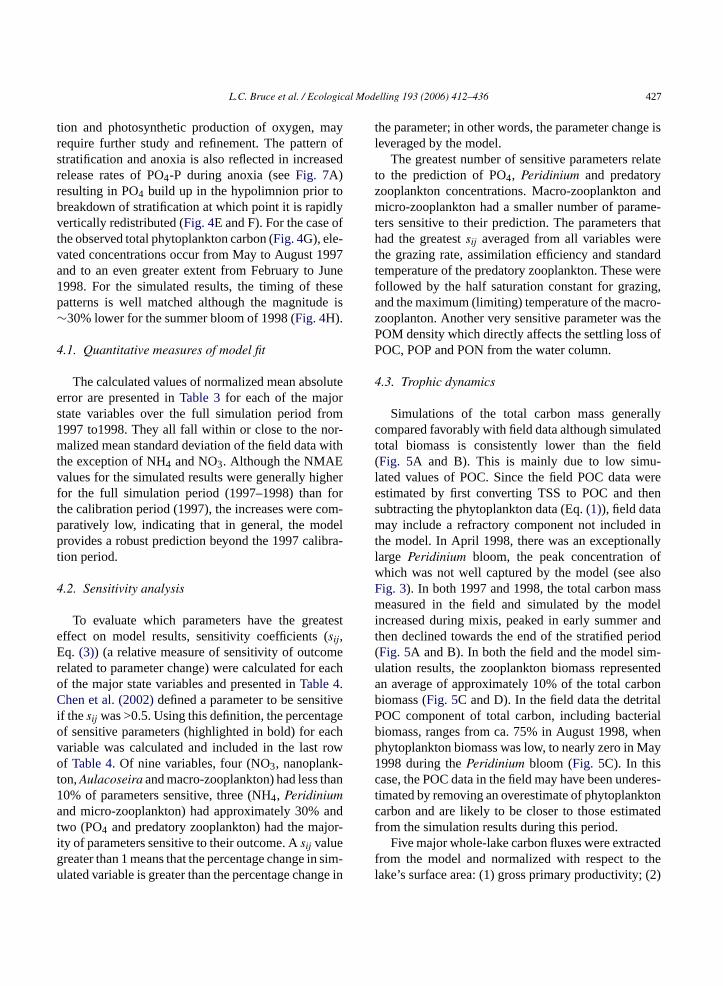
-m pth4 ately1 r( ts upi the

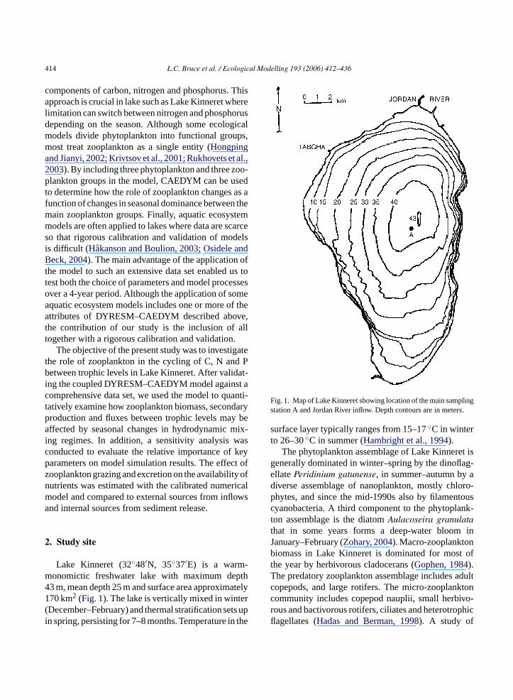
Fig. 1. Map of Lake Kinneret showing location of the main samplingstation A and Jordan River inflow. Depth contours are in meters.

surface layer typically ranges from 15–17◦C in winterto 26–30◦C in summer (Hambright et al., 1994).

The phytoplankton assemblage of Lake Kinneret isgenerally dominated in winter–spring by the dinoflag-ellatePeridinium gatunense, in summer–autumn by adiverse assemblage of nanoplankton, mostly chloro-phytes, and since the mid-1990s also by filamentouscyanobacteria. A third component to the phytoplank-ton assemblage is the diatomAulacoseira granulatathat in some years forms a deep-water bloom inJanuary–February (Zohary, 2004). Macro-zooplanktonbiomass in Lake Kinneret is dominated for most ofthe year by herbivorous cladocerans (Gophen, 1984).The predatory zooplankton assemblage includes adultcopepods, and large rotifers. The micro-zooplanktoncommunity includes copepod nauplii, small herbivo-rous and bactivorous rotifers, ciliates and heterotrophicflagellates (Hadas and Berman, 1998). A study of

ffected by seasonal changes in hydrodynamicng regimes. In addition, a sensitivity analysis wonducted to evaluate the relative importance ofarameters on model simulation results. The effeooplankton grazing and excretion on the availabilitutrients was estimated with the calibrated numeodel and compared to external sources from inflnd internal sources from sediment release.

. Study site

Lake Kinneret (32◦48′N, 35◦37′E) is a warmonomictic freshwater lake with maximum de3 m, mean depth 25 m and surface area approxim70 km2 (Fig. 1). The lake is vertically mixed in winteDecember–February) and thermal stratification sen spring, persisting for 7–8 months. Temperature in

L.C. Bruce et al. / Ecological Modelling 193 (2006) 412–436 415

stable carbon isotopes showed seasonal dietaryvariations of macro-zooplankton, with nanoplanktonas the predominant food source (Zohary et al., 1994).The major food sources for the micro-zooplanktonare bacteria and picophytoplankton for the smallerheterotrophic flagellates, and bacteria, heterotrophicflagellates and nanophytoplankton for the ciliates(Hadas and Berman, 1998; Madoni et al., 1990).

3. Methods

3.1. Model description

The model used in this study is a modified versionof the Computational Aquatic Ecosystem DynamicsModel (CAEDYM) coupled to the Dynamic Reser-voir Model (DYRESM). In DYRESM, the lake isrepresented as a series of homogeneous horizontalLagrangian layers of variable thickness; as inflowsand outflows enter or leave the lake, the affectedlayers expand or contract, respectively, and thoseabove move up or down to accommodate any volumechange. Mass, including that of the ecological statevariables, is adjusted conservatively each time layersmerge or are affected by inflows and outflows. Themain processes modeled in DYRESM are surface heat,mass and momentum transfers, mixed layer dynamics,hypolimnetic mixing, benthic boundary layer mixing,inflows and outflows. Local meteorological dataa e tos e toe andw othm facel r-f hata ectso andb byt rizedb ay,m s tot owc re-s sesi er(

Fig. 2. Schematic representation of: (A) the physical processesincluded in the physical model DYRESM (BBL: benthic boundarylayer; IC: internal cells; BC: benthic boundary layer cells) and (B)the carbon fluxes represented in the ecological model, CAEDYM.

The ecological model CAEDYM was set up inthe form of a nutrients–phytoplankton–zooplankton(‘N–P–Z’) model, but with resolution to the levelof individual species or groups of species (Griffinet al., 2000). In the present study, the model wasused to simulate phosphorus and nitrogen in bothparticulate organic and dissolved inorganic forms(POP and PO4, PON, NO3 and NH4), dissolvedoxygen (DO), particulate organic carbon (POC),dissolved organic carbon (DOC), three phytoplanktongroups and three zooplankton groups. The phy-toplankton community was simulated using threegroups in the model: “dinoflagellates”, representingP.gatunense, “diatoms”, representingA. granulata, and

re used to determine penetrative heating duhort-wave radiation and surface heat fluxes duvaporation, sensible heat, long-wave radiationind stress. The surface wind field introduces bomentum and turbulent kinetic energy to the sur

ayer contributing to vertical mixing. In addition to suace layer mixing, DYRESM includes algorithms tccount for internal mixing (encompassing the efff shear mixing energized by internal waves)enthic boundary layer (BBL) mixing (determined

he turbulent kinetic energy budget and parametey Lake Number and the Burger number). In this wass transfer is enabled from hypolimnetic layer

he thermocline region via the BBL. A schematic flhart of the operations performed in DYRESM is pented inFig. 2. A detailed description of the procesncluded in DYRESM is given byYeates and Imberg2004).

416 L.C. Bruce et al. / Ecological Modelling 193 (2006) 412–436

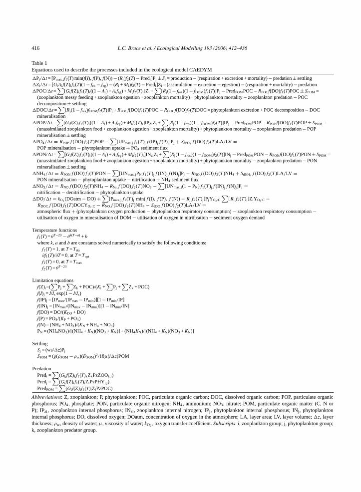
Table 1Equations used to describe the processes included in the ecological model CAEDYM

�Pj /�t = [Pmax,jf1(T) min(f(I), f(P), f(N)) − (Rj )f2(T) − Predj ]Pj ± Sj = production− (respiration + excretion + mortality)− predation± settling�Zi /�t = [GiAi f(Z)i f1(T)(1− fex − feg) − (Ri + Mi )f2(T) − Predi ]Zi = (assimilation− excretion− egestion)− (respiration + mortality)− predation�POC/�t =

∑[Gi f(Z)i f1(T)i ((1− Ai ) + Ai feg) + Mi f2(T)i ]Zi +

∑[Rj (1− fres)(1− fDOM)f2(T)]Pj − PredPOMPOC− RPOCf(DO)f1(T)POC± SPOM =

(zooplankton messy feeding + zooplankton egestion + zooplankton mortality) + phytoplankton mortality− zooplankton predation− POCdecomposition± settling

�DOC/�t =∑

[Rj (1− fres)fDOMf2(T)]Pj + RPOCf(DO)f2(T)POC− RDOCf(DO)f2(T)DOC = phytoplankton excretion + POC decomposition− DOCmineralisation

�POP/�t =∑

[Gi f(Z)i f1(T)i ((1− Ai ) + Ai feg) + Mi f2(T)i ]IPZiZi +∑

[Rj (1− fres)(1− fDOM)f2(T)]IPj − PredPOMPOP− RPOPf(DO)f1(T)POP± SPOM =(unassimilated zooplankton food + zooplankton egestion + zooplankton mortality) + phytoplankton mortality− zooplankton predation− POPmineralisation± settling

�PO4/�t = RPOPf (DO)f2(T )POP−∑

[UPmax,jf1(T )jf (IP)jf (P)j ]Pj + SdPO4f (DO)f2(T )LA/LV =POP mineralisation− phytoplankton uptake+ PO4 sediment flux

�PON/�t =∑

[Gi f(Z)i f1(T)i ((1− Ai ) + Ai feg) + Mi f2(T)i ]INziZi +∑

[Rj (1− fres)(1− fDOM)f2(T)]IN j − PredPOMPON− RPONf(DO)f1(T)PON± SPOM =(unassimilated zooplankton food + zooplankton egestion + zooplankton mortality) + phytoplankton mortality− zooplankton predation− PONmineralisation± settling

�NH4/�t = RPONf (DO)f1(T )PON−∑

[UNmax,jPNf1(T )jf (IN)jf (N)j ]Pj − RNOf (DO)f2(T )NH4 + SdNH4f (DO)f2(T )LA/LV =PON mineralisation− phytoplankton uptake− nitrification+ NH4 sediment flux

�NO3/�t = RNOf (DO)f2(T )NH4 − RN2f (DO)f2(T )NO3 −∑

[UNmax,j (1 − PN)f1(T )jf (IN)jf (N)j ]Pj =nitrification− denitrification− phytoplankton uptake

�DO/�t = kO2 (DOatm− DO) +∑

[Pmax,jf1(T )j min(f (I), f (P), f (N)) − Rjf2(T )j ]PjYO2:C

∑[Rif2(T )i ]ZiYO2:C −

RDOCf (DO)f1(T )DOCYO2:C − RNOf (DO)f2(T )NH4 − SdDOf (DO)f2(T )LA/LV =atmospheric flux+ (phytoplankton oxygen production− phytoplankton respiratory consumption)− zooplankton respiratory consumption−utilisation of oxygen in mineralisation of DOM− utilisation of oxygen in nitrification− sediment oxygen demand

Temperature functionsf1(T) = θT−20 − θk(T−a) + bwherek, a andb are constants solved numerically to satisfy the following conditions:

f1(T) = 1, atT = Tsta

∂f1(T)/∂T = 0, atT = Topt

f1(T) = 0, atT = Tmax

f2(T) = θT−20

Limitation equationsf(Z)i=(

∑Pj +

∑Zk + POC)/(Ki +

∑Pj +

∑Zk + POC)

f(I)j = I/Is exp(1− I/Is)f(IP)j = [IPmax/(IPmax− IPmin)][1 − IPmin/IP]f(IN)j = [INmax/(INmax− INmin)][1 − INmin/IN]f(DO) = DO/(KDO + DO)f(P) = PO4/(KP + PO4)f(N) = (NH4 + NO3)/(KN + NH4 + NO3)PN = (NH4NO3)/[(NH4 + KN)(NO3 + KN)] + (NH4KN)/[(NH4 + KN)(NO3 + KN)]

SettlingSj = (ws/�z)Pj

SPOM = (g(ρPOM − ρw)(DPOM)2/18µ)/�z)POM

PredationPredi =

∑(Gkf(Z)kf1(T)kZkPzZOOk,i)

Predj =∑

(Gi f(Z)i f1(T)iZiPzPHYi,j )PredPOM =

∑(Gi f(Z)i f1(T)iZiPzPOC)

Abbreviations: Z, zooplankton; P, phytoplankton; POC, particulate organic carbon; DOC, dissolved organic carbon; POP, particulate organicphosphorus; PO4, phosphate; PON, particulate organic nitrogen; NH4, ammonium; NO3, nitrate; POM, particulate organic matter (C, N orP); IPzi, zooplankton internal phosphorus; INzi, zooplankton internal nitrogen; IPj , phytoplankton internal phosphorus; INj , phytoplanktoninternal phosphorus; DO, dissolved oxygen; DOatm, concentration of oxygen in the atmosphere; LA, layer area; LV, layer volume;�z, layerthickness;ρw, density of water;µ, viscosity of water;kO2, oxygen transfer coefficient.Subscripts: i, zooplankton group; j, phytoplankton group;k, zooplankton predator group.

L.C. Bruce et al. / Ecological Modelling 193 (2006) 412–436 417

“nanoplankton” to account collectively for all otherphytoplankton. The total zooplankton biomass wasseparated in the model into predatory zooplanktoncomprised of adult stages of cyclopoid copepods andthe large rotiferAsplanchna, macro-zooplankton com-prised of cladocerans and juvenile (copepodid) stagesof copepods, and micro-zooplankton comprised ofcopepod nauplii, small rotifers and ciliates. CAEDYMuses a series of ordinary differential equations todescribe changes in concentrations of nutrients, detri-tus, dissolved oxygen, phytoplankton and zooplanktonas a function of environmental forcing and ecologicalinteractions for each Lagrangian layer represented byDYRESM. Details of the structure of this model aregiven inRobson and Hamilton (2004)andRomero etal. (2004). Physical transport of ecological variables iscarried out by DYRESM. The variables of irradiance,temperature, salinity and density are also passedto CAEDYM at each 1-h time step and used inequations to determine rates of change of biomassand chemical constituents for each of the ecologicalstate variable. A conceptual diagram of the majorecological components and interactions represented inthe model is shown inFig. 2 and the main equationsused in CAEDYM are listed inTable 1.

The major nutrient fluxes represented in CAEDYMare uptake of dissolved inorganic nutrients by phyto-plankton, release of dissolved nutrients from phyto-plankton excretion, grazing, egestion and excretion ofnutrients by zooplankton, nitrification and denitrifica-t s inp tiono entsf

yto-p cal-c ue tog enta-t andm tions

parameterized to represent the different physiologiesof each phytoplankton group (Table 2). Losses due tograzing by zooplankton are calculated by multiplyingthe food assimilation rate for each zooplankton groupby a preference factor for each food source.

Net zooplankton growth is calculated as a balancebetween food assimilation and losses from respira-tion, excretion, egestion, predation and mortality. Foodassimilation is calculated as the product of the maxi-mum potential rate of grazing, assimilation efficiencyand temperature and food concentration functions. Aconstant internal nutrient ratio is assumed for simplic-ity, and excretion of nutrients is used to maintain thisratio at each time step. Advective movement of zoo-plankton is carried out in DYRESM. The mechanism ofdiel vertical migration is not considered to be importantin the food web dynamics of Lake Kinneret (Easton andGophen, 2003) and so was not included in the model.

Bacteria were not modeled explicitly due to scarcityof data and lack of parameter information, but thenutrient pathways catalyzed by bacteria were includedin the mineralisation of the particulate organic pools(POC, POP and PON). Thus, the POC, POP and PONpools available for zooplankton grazing include bac-teria also. Fish were not modeled explicitly; however,grazing of fish on phytoplankton and predation of fishon zooplankton were accounted for by calibrating thephytoplankton and zooplankton mortality terms usingestimates of fish biomass and grazing and predationrates. Silica limitation of diatoms has not been observedi thisn dedi

3

tedac auset d for

TP n Lake

P Uni ature

K m−1

ion of inorganic nitrogen, sedimentation of nutrientarticulate form, bacterially catalyzed mineralisaf organic nutrients and release of dissolved nutri

rom bottom sediments (Table 1).Net change in carbon concentration for each ph

lankton state variable at each model time step isulated as the difference between the increment dross primary production and losses due to sedim

ion, grazing by zooplankton, respiration, excretionortality. These terms are calculated using equa

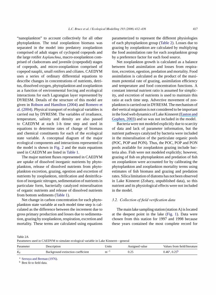
able 2Aarameters used in CAEDYM to simulate ecological variable i

arameter Description

d Background extinction coefficient

a Serruya and Berman (1976).b Best fit to field data.

n Lake Kinneret (Zohary, unpublished data), soutrient and its physiological effects were not inclu

n the model.

.2. Collection of field verification data

The main lake sampling station (station A) is locat the deepest point in the lake (Fig. 1). Data werehosen from this station for 1997 and 1998 bechese years contained the most complete recor

Kinneret—general

ts Assigned value Values from field/liter

0.25 0.46a, 0.25b

418 L.C. Bruce et al. / Ecological Modelling 193 (2006) 412–436

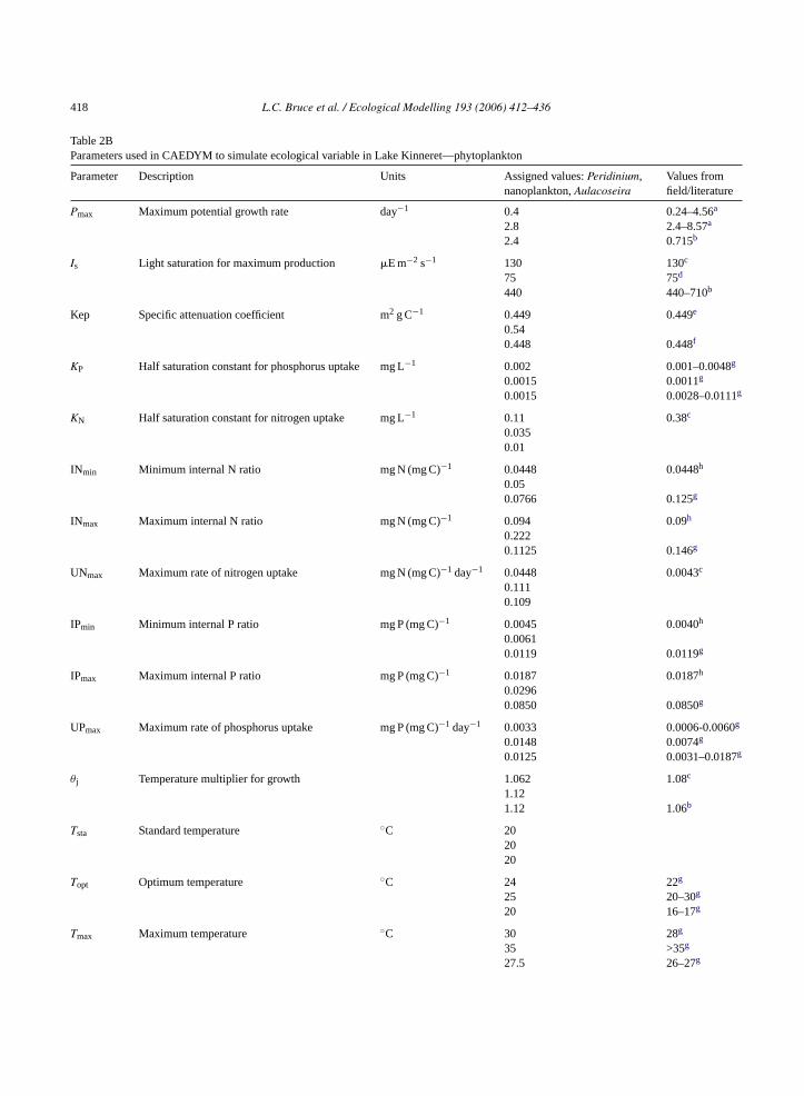
Table 2BParameters used in CAEDYM to simulate ecological variable in Lake Kinneret—phytoplankton

Parameter Description Units Assigned values:Peridinium,nanoplankton,Aulacoseira

Values fromfield/literature

Pmax Maximum potential growth rate day−1 0.4 0.24–4.56a

2.8 2.4–8.57a

2.4 0.715b

Is Light saturation for maximum production �E m−2 s−1 130 130c

75 75d

440 440–710b

Kep Specific attenuation coefficient m2 g C−1 0.449 0.449e

0.540.448 0.448f

KP Half saturation constant for phosphorus uptake mg L−1 0.002 0.001–0.0048g

0.0015 0.0011g

0.0015 0.0028–0.0111g

KN Half saturation constant for nitrogen uptake mg L−1 0.11 0.38c

0.0350.01

INmin Minimum internal N ratio mg N (mg C)−1 0.0448 0.0448h

0.050.0766 0.125g

INmax Maximum internal N ratio mg N (mg C)−1 0.094 0.09h

0.2220.1125 0.146g

UNmax Maximum rate of nitrogen uptake mg N (mg C)−1 day−1 0.0448 0.0043c

0.1110.109

IPmin Minimum internal P ratio mg P (mg C)−1 0.0045 0.0040h

0.00610.0119 0.0119g

IPmax Maximum internal P ratio mg P (mg C)−1 0.0187 0.0187h

0.02960.0850 0.0850g

UPmax Maximum rate of phosphorus uptake mg P (mg C)−1 day−1 0.0033 0.0006-0.0060g

0.0148 0.0074g

0.0125 0.0031–0.0187g

θj Temperature multiplier for growth 1.062 1.08c

1.121.12 1.06b

Tsta Standard temperature ◦C 202020

Topt Optimum temperature ◦C 24 22g

25 20–30g

20 16–17g

Tmax Maximum temperature ◦C 30 28g

35 >35g

27.5 26–27g

L.C. Bruce et al. / Ecological Modelling 193 (2006) 412–436 419

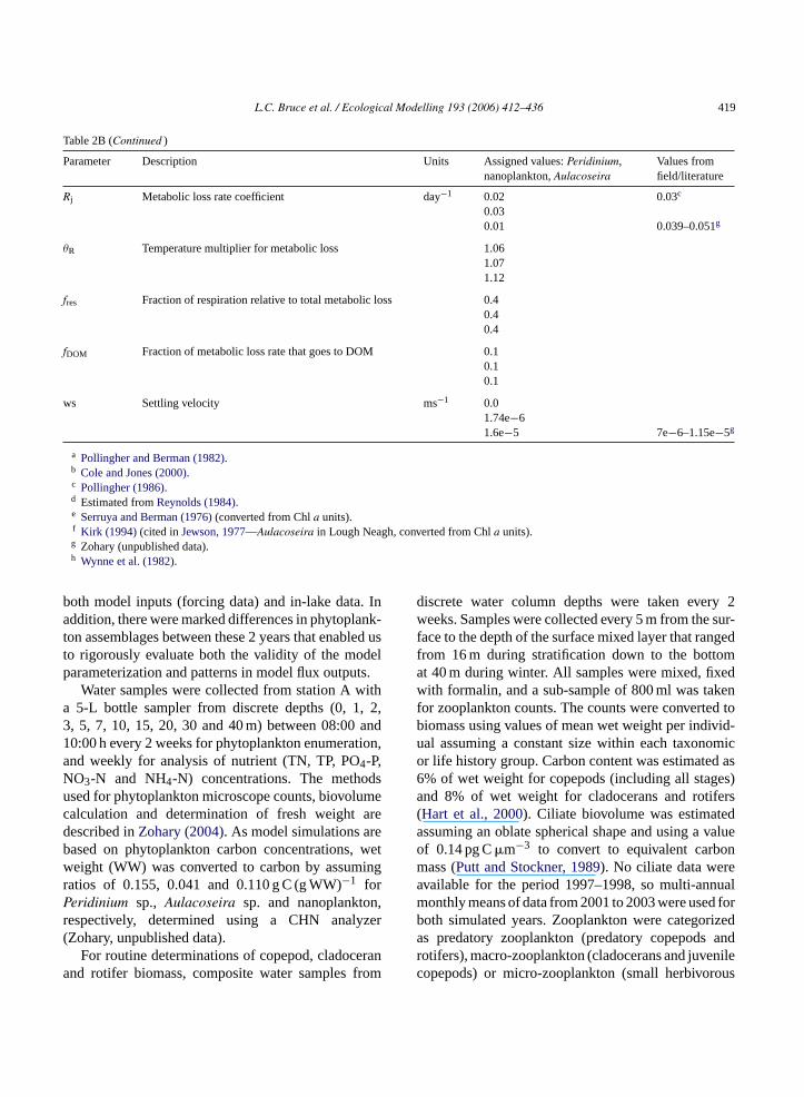
Table 2B (Continued )

Parameter Description Units Assigned values:Peridinium,nanoplankton,Aulacoseira

Values fromfield/literature

Rj Metabolic loss rate coefficient day−1 0.02 0.03c

0.030.01 0.039–0.051g

θR Temperature multiplier for metabolic loss 1.061.071.12

fres Fraction of respiration relative to total metabolic loss 0.40.40.4

fDOM Fraction of metabolic loss rate that goes to DOM 0.10.10.1

ws Settling velocity ms−1 0.01.74e−61.6e−5 7e−6–1.15e−5g

a Pollingher and Berman (1982).b Cole and Jones (2000).c Pollingher (1986).d Estimated fromReynolds (1984).e Serruya and Berman (1976)(converted from Chla units).f Kirk (1994) (cited inJewson, 1977—Aulacoseira in Lough Neagh, converted from Chla units).g Zohary (unpublished data).h Wynne et al. (1982).

both model inputs (forcing data) and in-lake data. Inaddition, there were marked differences in phytoplank-ton assemblages between these 2 years that enabled usto rigorously evaluate both the validity of the modelparameterization and patterns in model flux outputs.

Water samples were collected from station A witha 5-L bottle sampler from discrete depths (0, 1, 2,3, 5, 7, 10, 15, 20, 30 and 40 m) between 08:00 and10:00 h every 2 weeks for phytoplankton enumeration,and weekly for analysis of nutrient (TN, TP, PO4-P,NO3-N and NH4-N) concentrations. The methodsused for phytoplankton microscope counts, biovolumecalculation and determination of fresh weight aredescribed inZohary (2004). As model simulations arebased on phytoplankton carbon concentrations, wetweight (WW) was converted to carbon by assumingratios of 0.155, 0.041 and 0.110 g C (g WW)−1 forPeridinium sp., Aulacoseira sp. and nanoplankton,respectively, determined using a CHN analyzer(Zohary, unpublished data).

For routine determinations of copepod, cladoceranand rotifer biomass, composite water samples from

discrete water column depths were taken every 2weeks. Samples were collected every 5 m from the sur-face to the depth of the surface mixed layer that rangedfrom 16 m during stratification down to the bottomat 40 m during winter. All samples were mixed, fixedwith formalin, and a sub-sample of 800 ml was takenfor zooplankton counts. The counts were converted tobiomass using values of mean wet weight per individ-ual assuming a constant size within each taxonomicor life history group. Carbon content was estimated as6% of wet weight for copepods (including all stages)and 8% of wet weight for cladocerans and rotifers(Hart et al., 2000). Ciliate biovolume was estimatedassuming an oblate spherical shape and using a valueof 0.14 pg C�m−3 to convert to equivalent carbonmass (Putt and Stockner, 1989). No ciliate data wereavailable for the period 1997–1998, so multi-annualmonthly means of data from 2001 to 2003 were used forboth simulated years. Zooplankton were categorizedas predatory zooplankton (predatory copepods androtifers), macro-zooplankton (cladocerans and juvenilecopepods) or micro-zooplankton (small herbivorous

420 L.C. Bruce et al. / Ecological Modelling 193 (2006) 412–436

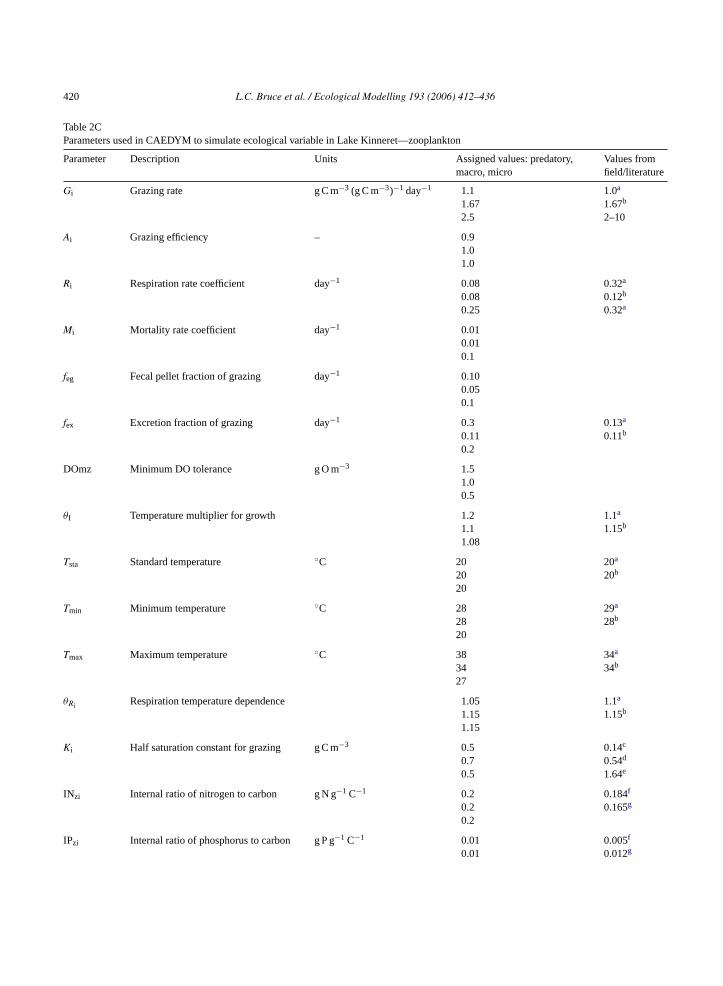
Table 2CParameters used in CAEDYM to simulate ecological variable in Lake Kinneret—zooplankton

Parameter Description Units Assigned values: predatory,macro, micro

Values fromfield/literature

Gi Grazing rate g C m−3 (g C m−3)−1 day−1 1.1 1.0a

1.67 1.67b

2.5 2–10

Ai Grazing efficiency – 0.91.01.0

Ri Respiration rate coefficient day−1 0.08 0.32a

0.08 0.12b

0.25 0.32a

Mi Mortality rate coefficient day−1 0.010.010.1

feg Fecal pellet fraction of grazing day−1 0.100.050.1

fex Excretion fraction of grazing day−1 0.3 0.13a

0.11 0.11b

0.2

DOmz Minimum DO tolerance g O m−3 1.51.00.5

θI Temperature multiplier for growth 1.2 1.1a

1.1 1.15b

1.08

Tsta Standard temperature ◦C 20 20a

20 20b

20

Tmin Minimum temperature ◦C 28 29a

28 28b

20

Tmax Maximum temperature ◦C 38 34a

34 34b

27

θRi Respiration temperature dependence 1.05 1.1a

1.15 1.15b

1.15

Ki Half saturation constant for grazing g C m−3 0.5 0.14c

0.7 0.54d

0.5 1.64e

INzi Internal ratio of nitrogen to carbon g N g−1 C−1 0.2 0.184f

0.2 0.165g

0.2

IPzi Internal ratio of phosphorus to carbon g P g−1 C−1 0.01 0.005f

0.01 0.012g

L.C. Bruce et al. / Ecological Modelling 193 (2006) 412–436 421

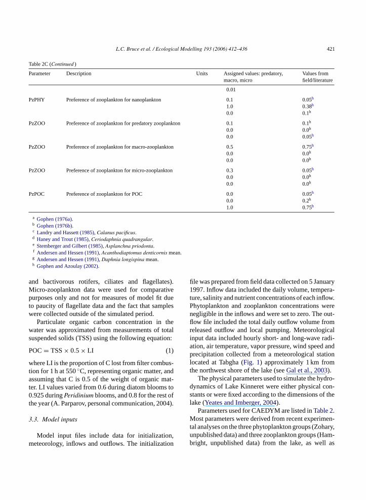
Table 2C (Continued )

Parameter Description Units Assigned values: predatory,macro, micro

Values fromfield/literature

0.01

PzPHY Preference of zooplankton for nanoplankton 0.1 0.05h

1.0 0.38h

0.0 0.1h

PzZOO Preference of zooplankton for predatory zooplankton 0.1 0.1h

0.0 0.0h

0.0 0.05h

PzZOO Preference of zooplankton for macro-zooplankton 0.5 0.75h

0.0 0.0h

0.0 0.0h

PzZOO Preference of zooplankton for micro-zooplankton 0.3 0.05h

0.0 0.0h

0.0 0.0h

PzPOC Preference of zooplankton for POC 0.0 0.05h

0.0 0.2h

1.0 0.75h

a Gophen (1976a).b Gophen (1976b).c Landry and Hassett (1985), Calanus pacificus.d Haney and Trout (1985), Ceriodaphnia quadrangular.e Stemberger and Gilbert (1985), Asplanchna priodonta.f Andersen and Hessen (1991), Acanthodiaptomus denticornis mean.g Andersen and Hessen (1991), Daphnia longispina mean.h Gophen and Azoulay (2002).

and bactivorous rotifers, ciliates and flagellates).Micro-zooplankton data were used for comparativepurposes only and not for measures of model fit dueto paucity of flagellate data and the fact that sampleswere collected outside of the simulated period.

Particulate organic carbon concentration in thewater was approximated from measurements of totalsuspended solids (TSS) using the following equation:

POC= TSS× 0.5 × LI (1)

where LI is the proportion of C lost from filter combus-tion for 1 h at 550◦C, representing organic matter, andassuming that C is 0.5 of the weight of organic mat-ter. LI values varied from 0.6 during diatom blooms to0.925 duringPeridinium blooms, and 0.8 for the rest ofthe year (A. Parparov, personal communication, 2004).

3.3. Model inputs

Model input files include data for initialization,meteorology, inflows and outflows. The initialization

file was prepared from field data collected on 5 January1997. Inflow data included the daily volume, tempera-ture, salinity and nutrient concentrations of each inflow.Phytoplankton and zooplankton concentrations werenegligible in the inflows and were set to zero. The out-flow file included the total daily outflow volume fromreleased outflow and local pumping. Meteorologicalinput data included hourly short- and long-wave radi-ation, air temperature, vapor pressure, wind speed andprecipitation collected from a meteorological stationlocated at Tabgha (Fig. 1) approximately 1 km fromthe northwest shore of the lake (seeGal et al., 2003).

The physical parameters used to simulate the hydro-dynamics of Lake Kinneret were either physical con-stants or were fixed according to the dimensions of thelake (Yeates and Imberger, 2004).

Parameters used for CAEDYM are listed inTable 2.Most parameters were derived from recent experimen-tal analyses on the three phytoplankton groups (Zohary,unpublished data) and three zooplankton groups (Ham-bright, unpublished data) from the lake, as well as

422 L.C. Bruce et al. / Ecological Modelling 193 (2006) 412–436

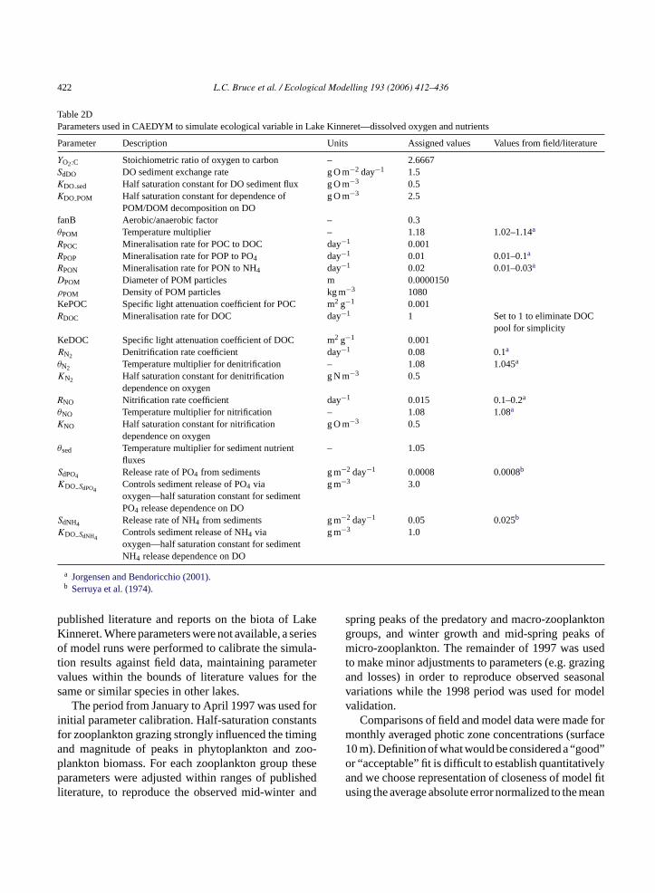
Table 2DParameters used in CAEDYM to simulate ecological variable in Lake Kinneret—dissolved oxygen and nutrients

Parameter Description Units Assigned values Values from field/literature

YO2:C Stoichiometric ratio of oxygen to carbon – 2.6667SdDO DO sediment exchange rate g O m−2 day−1 1.5KDO sed Half saturation constant for DO sediment flux g O m−3 0.5KDO POM Half saturation constant for dependence of

POM/DOM decomposition on DOg O m−3 2.5

fanB Aerobic/anaerobic factor – 0.3θPOM Temperature multiplier – 1.18 1.02–1.14a

RPOC Mineralisation rate for POC to DOC day−1 0.001RPOP Mineralisation rate for POP to PO4 day−1 0.01 0.01–0.1a

RPON Mineralisation rate for PON to NH4 day−1 0.02 0.01–0.03a

DPOM Diameter of POM particles m 0.0000150ρPOM Density of POM particles kg m−3 1080KePOC Specific light attenuation coefficient for POC m2 g−1 0.001RDOC Mineralisation rate for DOC day−1 1 Set to 1 to eliminate DOC

pool for simplicityKeDOC Specific light attenuation coefficient of DOC m2 g−1 0.001RN2 Denitrification rate coefficient day−1 0.08 0.1a

θN2 Temperature multiplier for denitrification – 1.08 1.045a

KN2 Half saturation constant for denitrificationdependence on oxygen

g N m−3 0.5

RNO Nitrification rate coefficient day−1 0.015 0.1–0.2a

θNO Temperature multiplier for nitrification – 1.08 1.08a

KNO Half saturation constant for nitrificationdependence on oxygen

g O m−3 0.5

θsed Temperature multiplier for sediment nutrientfluxes

– 1.05

SdPO4 Release rate of PO4 from sediments g m−2 day−1 0.0008 0.0008b

KDO SdPO4Controls sediment release of PO4 viaoxygen—half saturation constant for sedimentPO4 release dependence on DO

g m−3 3.0

SdNH4 Release rate of NH4 from sediments g m−2 day−1 0.05 0.025b

KDO SdNH4Controls sediment release of NH4 viaoxygen—half saturation constant for sedimentNH4 release dependence on DO

g m−3 1.0

a Jorgensen and Bendoricchio (2001).b Serruya et al. (1974).

published literature and reports on the biota of LakeKinneret. Where parameters were not available, a seriesof model runs were performed to calibrate the simula-tion results against field data, maintaining parametervalues within the bounds of literature values for thesame or similar species in other lakes.

The period from January to April 1997 was used forinitial parameter calibration. Half-saturation constantsfor zooplankton grazing strongly influenced the timingand magnitude of peaks in phytoplankton and zoo-plankton biomass. For each zooplankton group theseparameters were adjusted within ranges of publishedliterature, to reproduce the observed mid-winter and

spring peaks of the predatory and macro-zooplanktongroups, and winter growth and mid-spring peaks ofmicro-zooplankton. The remainder of 1997 was usedto make minor adjustments to parameters (e.g. grazingand losses) in order to reproduce observed seasonalvariations while the 1998 period was used for modelvalidation.

Comparisons of field and model data were made formonthly averaged photic zone concentrations (surface10 m). Definition of what would be considered a “good”or “acceptable” fit is difficult to establish quantitativelyand we choose representation of closeness of model fitusing the average absolute error normalized to the mean

L.C. Bruce et al. / Ecological Modelling 193 (2006) 412–436 423

(NMAE; Alewell and Manderscheid, 1998):

NMAE =∑n

t=1(|st − ot|)no

, (2)

wherest is the simulated value at timet, ot the observedvalue at timet, o the mean of the observed values overthe simulation period andn is the number of observedvalues. NMAE is a measure of the absolute deviation ofsimulated values from observations, normalized to themean; a value of zero indicates perfect agreement andgreater than zero an average fraction of the discrepancynormalized to the mean. Since an acceptable fit dependson the scatter of the observed data, we calculated, fromthe field data for each state variable, a standard devia-tion from monthly averages. As a comparison to overallmodel fit, these monthly standard deviations were thenaveraged over the simulation period and normalizedto the mean (seeTable 3). Model fit was consideredacceptable when the simulated NMAE’s fell within orclose to one standard deviation of the observed monthlyaverage field data.

Although the NMAE method gives useful quanti-tative information about model performance, it maymisrepresent the fit in cases where the mean is verysmall compared with a short-term peak or bloom(Alewell and Manderscheid, 1998). Values of NMAEwere therefore combined with qualitative graphicalcomparisons in evaluating the success of the calibra-tion procedure.

A sensitivity analysis was performed on each of theC h

TR ionsa 8

V

D 6)N )N )P )N 1)P )A )P 46)M 0)M

A 5)

T de ovet

parameter by±10% or by±0.01 in the case of thetemperature multipliers. Sensitivity coefficients (sij) toassess the relative sensitivity of variablei to parameterj were calculated according toChen et al. (2002):

sij = �ci/ci

�βj/βj

(3)

where�cj is the change in variablei from the referencevalueci and�βj is the change in parameterj from thereference valueβj. The calculations were made for eachof the major state variables taking the daily mean photicdepth concentrations averaged over the full simulationperiod.

4. Results

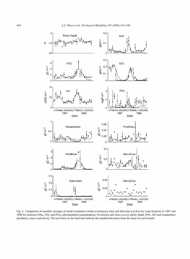
Dissolved oxygen in the upper 10 m measured inthe field is elevated through the first 6 months of bothyears, with a peak in May–April corresponding toincreased phytoplankton biomass as a result ofPeri-dinium blooms (Fig. 3). The simulated data show asimilar pattern although peak values are slightly lowerthan in the field. The inorganic nitrogen field data forthe upper 10 m of water column show a strong sea-sonal pattern with increased concentrations in the win-ter months following the breakdown in stratification,and low concentrations during the summer stratifiedperiod (Fig. 3). The NO3 peak and subsequent declinein the field data followed a similar sequence, but withaTN upo d.N inor-g take( at-tsiT edt 98a houtt dc ioni sim-u thes ded

AEDYM parameters listed inTable 2, adjusting eac

able 3esults of normalized mean absolute error (NMAE) calculatpplied to compare simulated to field data for years 1997–199

ariable NMAE S.D./mean

issolved oxygen 0.07 (0.09) 0.07 (0.0H4 0.66 (0.68) 0.40 (0.44O3 0.43 (0.32) 0.27 (0.20O4 0.81 (0.81) 0.66 (0.91anoplankton 0.50 (0.41) 0.37 (0.4eridinium 0.40 (0.51) 0.41 (0.44ulacoseira 0.79 (0.49) 0.68 (0.89redatory zooplankton 0.59 (0.51) 0.50 (0.acro-zooplankton 0.46 (0.35) 0.31 (0.2icro-zooplankton 0.85 (0.88) –

verage 0.52 (0.46) 0.41 (0.4

he values in parentheses represent the same calculations mahe 1997 calibration period.

r

1–2 month phase lag compared with NH4 (Fig. 3).he lag may be explained by nitrification of NH4 toO3 at turnover, following the progressive buildf NH4 in the hypolimnion during the stratified perioO3 subsequently declined in the surface layer asanic nutrients were depleted through biological upFig. 3). The simulated results showed a similar pern although the summer decline of NO3 in 1997 waslower than observed in the field and the NH4 peakn the 1997–1998 winter was slightly delayed (Fig. 3).he PO4 field data varied irregularly in 1997, declin

o low concentrations in the first 3 months of 19nd then showed elevated concentrations throug

he remainder of 1998 (Fig. 3). A period of increaseoncentration following the breakdown of stratificatn December 1997 was captured with the modellations, as well as the elevated concentrations inecond half of 1998, but the model otherwise ten

424 L.C. Bruce et al. / Ecological Modelling 193 (2006) 412–436

Fig. 3. Comparison of monthly averages of model simulation results (continuous line) and field data (circles) for Lake Kinneret in 1997 and1998 for nutrients (NH4, NO3 and PO4), phytoplankton (nanoplankton,Peridinium andAulacoseira), photic depth, POC, DO and zooplankton(predatory, macro and micro). The error bars on the field data indicate the standard deviation from the mean for each month.

L.C. Bruce et al. / Ecological Modelling 193 (2006) 412–436 425

to underestimate PO4 concentrations (Fig. 3). Despitethis discrepancy, the simulation results of the major (interm of biomass) phytoplankton species (nanoplanktonandPeridinium) generally closely followed the trendsin the field data.

The nanoplankton field and simulated data exhibita similar pattern to the PO4 data, with concentrationsthat were variable in 1997, decreased in early 1998 andwere then elevated for the remainder of 1998 (Fig. 3).ThePeridinium field data show two peaks: one in 1997and one in 1998 (Fig. 3). The 1997 peak occurred later(June–July) and was seven times lower than the peakin June 1998 which was the end-point of a continu-ous increase from February 1998 (Fig. 3). The othermajor difference between the years was that, althoughsomePeridinium biomass persisted through the secondhalf of 1997, there was little biomass in the secondhalf of 1998. These patterns were captured well inthe simulated data (Fig. 3). Large increases inAulaco-seira biomass occurred in January and February of both1997 and 1998. The simulated results did not repro-duce the bloom in 1998 but the C-biomass contributedby Aulacoseira was small (3% of total) and of lesserimportance to the role of zooplankton, that generallydo not graze this large filamentous diatom (Fig. 3). Thetiming and magnitude of the peaks may be related toresuspension of resting cells caused by high turbulence(Zohary, 2004) while the decline may be related to there-establishment of the stratification and enhanced sed-imentation losses of cells. Resuspension of resting cellsw thea dr an-u os

in-n short-d omA ev buttT erea nk-t rnsi atedm d int ldd ass

measurement for years 2001–2003, so there is no inter-annual variation (Fig. 3) but there is a peak in concen-tration for the months of April and May. These peakswere not captured in the model data, and the simu-lated concentrations for the remainder of both yearswere lower than the field data (Fig. 3). Although thecontribution of micro-zooplankton to total zooplank-ton biomass is small, this group has high growth andexcretion rates, so their contribution to lake nutrientfluxes is most probably underestimated.

It is possible that discrepancies between model andfield data may be the result of misrepresentation offield data associated with bias from sampling concen-trated patches of zooplankton (seeYacobi et al., 1993).The errors associated with spatial and temporal vari-ations are reflected in the error bars representing thestandard deviation calculated from samples taken atdifferent times in the lake (Fig. 3); high spatial variabil-ity is evident where the standard deviation exceeds themean value (e.g. predatory zooplankton in June 1998).In the cases where spatial variation is not so evident(e.g.Peridinium, January–December 1997), simulatedand observed data are generally in good agreement. Inthese cases, the use of a spatially averaged model ismore appropriate.

In summary, the model appeared to simulate allthe variables within the bounds of the scatter in thefield data. The only major exception to this was micro-zooplankton where the model simulations were con-sistently too low after the initial calibration period. Ase rac-t vinga diffi-c hasi hem e.

thata m-b tely2 byt dedv sedo ures( ngt thedD tion,d mp-

as not simulated in the model, which may explainbsence of anAulacoseira bloom in the 1998 simulateesults, while the initial conditions prescribed for Jary 1997 (0.025 g C m−3) stimulated a bloom prior ttratification.

Biomass of predatory zooplankton in Lake Keret showed reasonable scatter punctuated by auration peak in April 1997 and a larger peak frpril to May 1998 (Fig. 3). The magnitude of thesariations was captured by the model simulationshe peak in June 1998 was not reproduced (Fig. 3).he field data for the macro-zooplankton biomass wlmost 10 times higher than for the predatory zoopla

on. It is difficult to discern obvious seasonal patten the field data although concentrations were elev

id-summer and mid-winter, which were capturehe simulations (Fig. 3). The micro-zooplankton fieata were compiled by averaging monthly biom

xplained above, the micro-zooplankton were chaerized by a high turnover of biomass so that achiebalance between growth rate and respiration wasult. Current data collection of micro-zooplanktonmproved and future work will focus on the role of t

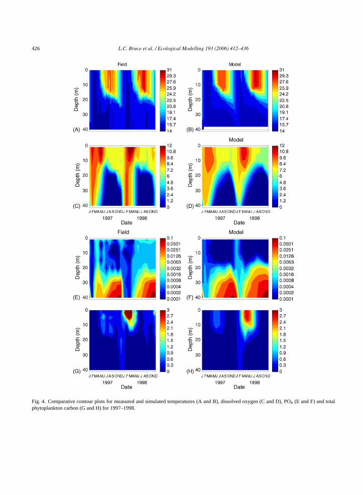
icro-zooplankton in the nutrient cycles of the lakIn both 1997 and 1998, the field data indicate

noxia occurs in the hypolimnion from June to Noveer or December, below a depth of approxima0 m (Fig. 4C). This pattern was well reproduced

he model although the oxygen depletion extenertically faster in the field than in the model. Ban the comparison of field and simulated temperatFig. 4A and B, respectively), the extent of mixihrough the water column is well reproduced, butiscrepancy in the oxygen contour plots (Fig. 4C and) suggests that the water column oxygen depleetermined through interactions of mixing, consu

426 L.C. Bruce et al. / Ecological Modelling 193 (2006) 412–436

Fig. 4. Comparative contour plots for measured and simulated temperatures (A and B), dissolved oxygen (C and D), PO4 (E and F) and totalphytoplankton carbon (G and H) for 1997–1998.

L.C. Bruce et al. / Ecological Modelling 193 (2006) 412–436 427

tion and photosynthetic production of oxygen, mayrequire further study and refinement. The pattern ofstratification and anoxia is also reflected in increasedrelease rates of PO4-P during anoxia (seeFig. 7A)resulting in PO4 build up in the hypolimnion prior tobreakdown of stratification at which point it is rapidlyvertically redistributed (Fig. 4E and F). For the case ofthe observed total phytoplankton carbon (Fig. 4G), ele-vated concentrations occur from May to August 1997and to an even greater extent from February to June1998. For the simulated results, the timing of thesepatterns is well matched although the magnitude is∼30% lower for the summer bloom of 1998 (Fig. 4H).

4.1. Quantitative measures of model fit

The calculated values of normalized mean absoluteerror are presented inTable 3for each of the majorstate variables over the full simulation period from1997 to1998. They all fall within or close to the nor-malized mean standard deviation of the field data withthe exception of NH4 and NO3. Although the NMAEvalues for the simulated results were generally higherfor the full simulation period (1997–1998) than forthe calibration period (1997), the increases were com-paratively low, indicating that in general, the modelprovides a robust prediction beyond the 1997 calibra-tion period.

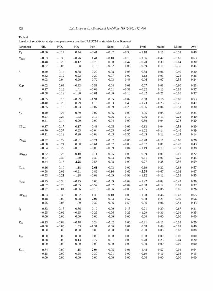
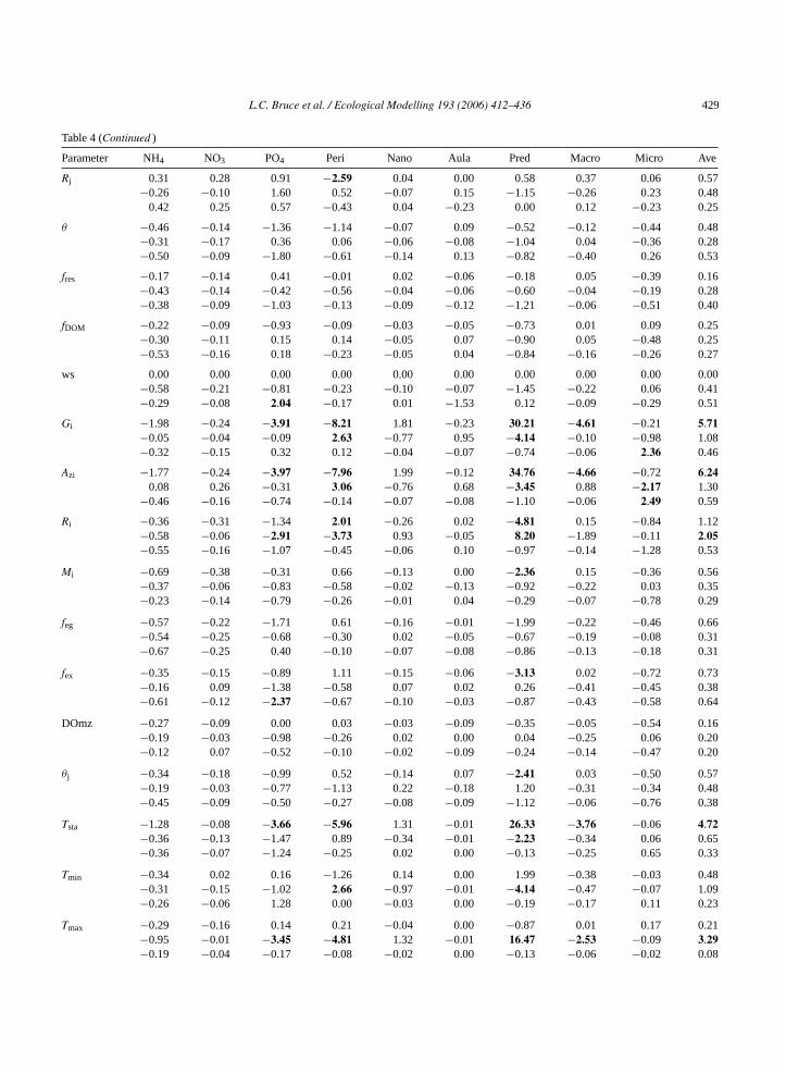
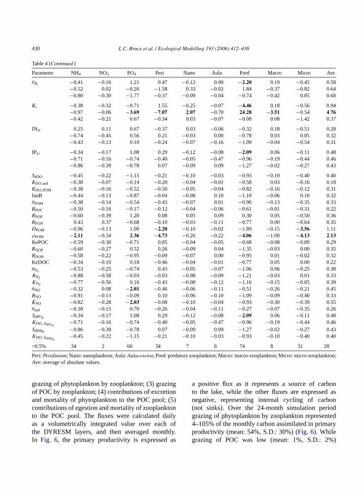
4.2. Sensitivity analysis

ateste (E mer eachoC tivei ageo achv rowo -t an1a andt jor-ig n sim-u ge in

the parameter; in other words, the parameter change isleveraged by the model.

The greatest number of sensitive parameters relateto the prediction of PO4, Peridinium and predatoryzooplankton concentrations. Macro-zooplankton andmicro-zooplankton had a smaller number of parame-ters sensitive to their prediction. The parameters thathad the greatestsij averaged from all variables werethe grazing rate, assimilation efficiency and standardtemperature of the predatory zooplankton. These werefollowed by the half saturation constant for grazing,and the maximum (limiting) temperature of the macro-zooplanton. Another very sensitive parameter was thePOM density which directly affects the settling loss ofPOC, POP and PON from the water column.

4.3. Trophic dynamics

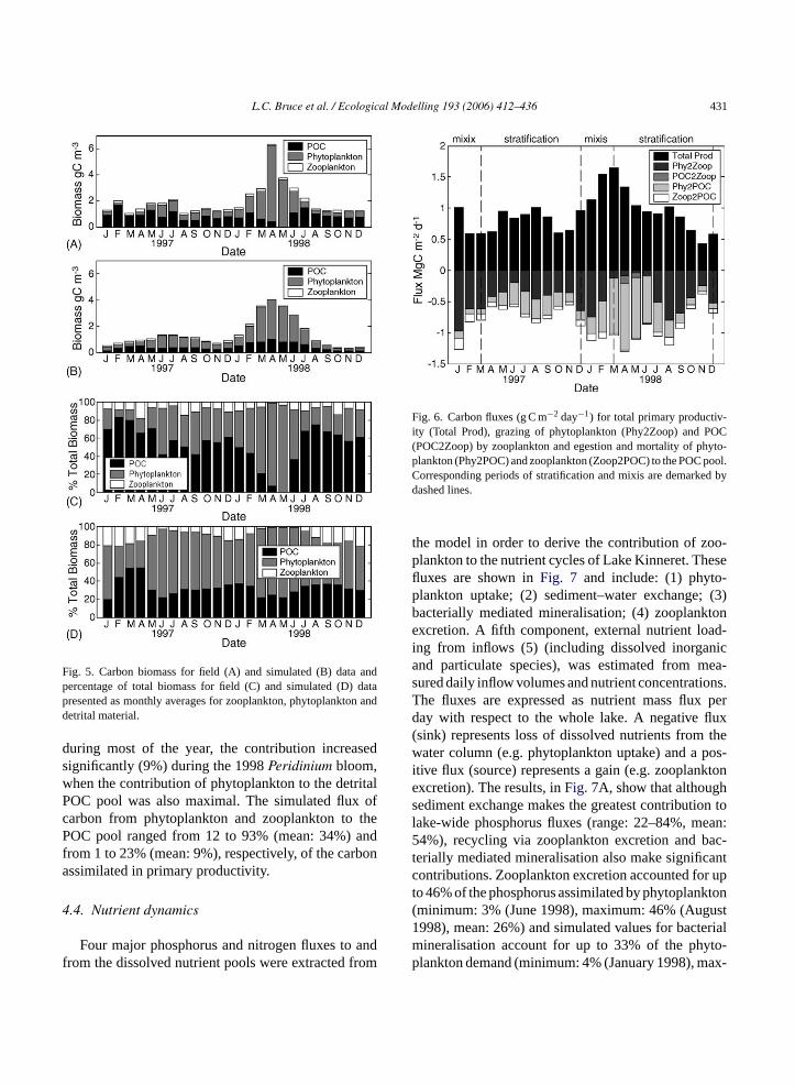
Simulations of the total carbon mass generallycompared favorably with field data although simulatedtotal biomass is consistently lower than the field(Fig. 5A and B). This is mainly due to low simu-lated values of POC. Since the field POC data wereestimated by first converting TSS to POC and thensubtracting the phytoplankton data (Eq.(1)), field datamay include a refractory component not included inthe model. In April 1998, there was an exceptionallylarge Peridinium bloom, the peak concentration ofwhich was not well captured by the model (see alsoFig. 3). In both 1997 and 1998, the total carbon massm odeli andt riod( m-u nteda bonb talP rialb henp ay1c eres-t tonc atedf

tedf thel (2)

To evaluate which parameters have the greffect on model results, sensitivity coefficientssij,q. (3)) (a relative measure of sensitivity of outco

elated to parameter change) were calculated forf the major state variables and presented inTable 4.hen et al. (2002)defined a parameter to be sensi

f the sij was >0.5. Using this definition, the percentf sensitive parameters (highlighted in bold) for eariable was calculated and included in the lastf Table 4. Of nine variables, four (NO3, nanoplank

on,Aulacoseira and macro-zooplankton) had less th0% of parameters sensitive, three (NH4, Peridiniumnd micro-zooplankton) had approximately 30%

wo (PO4 and predatory zooplankton) had the maty of parameters sensitive to their outcome. Asij valuereater than 1 means that the percentage change ilated variable is greater than the percentage chan

easured in the field and simulated by the mncreased during mixis, peaked in early summerhen declined towards the end of the stratified peFig. 5A and B). In both the field and the model silation results, the zooplankton biomass represen average of approximately 10% of the total cariomass (Fig. 5C and D). In the field data the detriOC component of total carbon, including bacteiomass, ranges from ca. 75% in August 1998, whytoplankton biomass was low, to nearly zero in M998 during thePeridinium bloom (Fig. 5C). In thisase, the POC data in the field may have been undimated by removing an overestimate of phytoplankarbon and are likely to be closer to those estimrom the simulation results during this period.

Five major whole-lake carbon fluxes were extracrom the model and normalized with respect toake’s surface area: (1) gross primary productivity;

428 L.C. Bruce et al. / Ecological Modelling 193 (2006) 412–436

Table 4Results of sensitivity analysis on parameters used in CAEDYM to simulate Lake Kinneret

Parameter NH4 NO3 PO4 Peri Nano Aula Pred Macro Micro Ave

Kd −0.36 −0.14 0.44 −0.41 −0.07 −0.38 −1.18 0.11 −0.51 0.40

Pmax −0.63 −0.35 −0.76 1.41 −0.10 −0.10 −1.66 −0.47 −0.18 0.63−0.48 −0.25 −0.12 −0.75 0.00 −0.47 −0.20 0.30 −0.14 0.30−0.27 −0.06 1.08 0.13 −0.02 1.06 −0.89 0.11 −0.35 0.44

Is −0.40 −0.14 −0.38 −0.22 −0.08 −0.08 −0.88 −0.06 −0.49 0.30−0.32 −0.12 0.22 0.20 −0.07 0.00 −1.12 −0.03 −0.24 0.26

0.03 0.04 −0.20 −0.72 0.03 −0.43 0.06 0.07 −0.55 0.24

Kep −0.02 0.06 −0.63 −0.53 0.04 0.08 0.07 0.03 −0.60 0.230.17 0.13 1.41 −0.02 0.01 −0.31 −0.32 0.13 −0.83 0.37

−0.58 −0.19 −1.30 −0.01 −0.06 −0.10 −0.82 −0.21 −0.05 0.37

KP −0.05 0.15 −0.99 −1.91 0.05 −0.02 0.58 0.16 −0.88 0.53−0.40 −0.26 0.29 1.13 −0.03 0.40 −1.23 −0.23 −0.26 0.47−0.35 −0.18 −0.23 −0.07 −0.09 −0.29 −0.96 −0.04 −0.51 0.30

KN −0.40 −0.24 −0.69 0.07 −0.06 −0.02 −1.06 0.08 −0.43 0.34−0.27 −0.28 −1.53 0.16 −0.06 −0.10 −0.86 −0.13 −0.24 0.40−0.41 −0.14 0.20 −0.09 −0.04 0.09 −0.89 −0.04 −0.78 0.30

INmin −0.37 −0.17 0.17 −0.48 −0.05 −0.09 −0.83 0.04 −0.53 0.30−0.70 −0.37 0.65 −0.04 −0.05 −0.07 −1.02 −0.14 −0.46 0.39−0.11 −0.12 0.20 −0.08 0.03 −0.35 −0.05 0.12 −0.24 0.14

INmax −0.32 −0.22 −0.31 −0.21 −0.02 −0.06 −0.48 −0.11 −0.60 0.26−0.68 −0.74 0.80 −0.61 −0.07 −0.08 −0.67 0.01 −0.20 0.43−0.54 −0.22 −0.61 −0.03 −0.09 0.04 −1.19 −0.19 −0.51 0.38

UNmax −0.62 −0.26 −0.10 −0.11 −0.05 0.05 −0.59 0.01 0.16 0.22−0.67 −0.46 1.30 −0.40 −0.04 0.01 −0.81 −0.01 −0.28 0.44−0.44 −0.18 −2.28 −0.58 −0.08 −0.09 −0.77 −0.38 −0.56 0.59

IPmin −0.16 0.10 1.18 −2.61 −0.03 0.02 −0.19 0.22 −0.63 0.57−0.58 0.03 −0.81 0.82 −0.16 0.62 −2.28 −0.67 −0.02 0.67−0.53 −0.21 −1.28 −0.09 −0.09 −0.98 −1.12 −0.12 −0.53 0.55

IPmax −0.75 −0.30 −0.45 0.06 −0.09 −0.09 −1.27 −0.02 −0.47 0.39−0.67 −0.20 −0.85 −0.52 −0.07 −0.04 −0.88 −0.12 0.01 0.37−0.27 −0.04 −0.56 −0.18 −0.06 −0.03 −1.05 −0.06 0.05 0.26

UPmax −0.83 −0.35 −0.52 1.30 −0.10 0.00 −1.88 −0.46 −0.43 0.65−0.18 0.09 −0.98 −2.04 0.04 −0.52 0.38 0.21 −0.59 0.56−0.25 −0.05 −1.09 −0.32 −0.06 0.50 −0.96 −0.06 −0.54 0.43

θj −0.33 −0.15 0.86 −0.12 0.00 −0.15 −0.21 0.29 −0.67 0.31−0.55 −0.09 −0.35 −0.25 −0.06 0.23 −1.29 −0.36 −0.01 0.35

0.00 0.00 0.00 0.00 0.00 0.00 0.00 0.00 0.00 0.00

Tsta −0.23 −0.08 −0.78 0.24 −0.02 0.00 −0.31 −0.11 −0.03 0.20−0.08 −0.05 1.53 −1.31 0.06 0.01 0.58 0.49 −0.01 0.46

0.00 0.00 0.00 0.00 0.00 0.00 0.00 0.00 0.00 0.00

Topt 0.00 0.00 0.00 0.00 0.00 0.00 0.00 0.00 0.00 0.00−0.28 −0.08 −0.13 −0.77 0.01 0.00 0.28 0.23 0.04 0.20

0.00 0.00 0.00 0.00 0.00 0.00 0.00 0.00 0.00 0.00

Tmax −0.34 −0.09 −1.15 2.06 −0.05 −0.01 −1.48 −0.57 −0.01 0.64−0.15 0.00 0.58 −0.30 −0.01 0.00 −0.10 −0.16 −0.03 0.15

0.00 0.00 0.00 0.00 0.00 0.00 0.00 0.00 0.00 0.00

L.C. Bruce et al. / Ecological Modelling 193 (2006) 412–436 429

Table 4 (Continued )

Parameter NH4 NO3 PO4 Peri Nano Aula Pred Macro Micro Ave

Rj 0.31 0.28 0.91 −2.59 0.04 0.00 0.58 0.37 0.06 0.57−0.26 −0.10 1.60 0.52 −0.07 0.15 −1.15 −0.26 0.23 0.48

0.42 0.25 0.57 −0.43 0.04 −0.23 0.00 0.12 −0.23 0.25

θ −0.46 −0.14 −1.36 −1.14 −0.07 0.09 −0.52 −0.12 −0.44 0.48−0.31 −0.17 0.36 0.06 −0.06 −0.08 −1.04 0.04 −0.36 0.28−0.50 −0.09 −1.80 −0.61 −0.14 0.13 −0.82 −0.40 0.26 0.53

fres −0.17 −0.14 0.41 −0.01 0.02 −0.06 −0.18 0.05 −0.39 0.16−0.43 −0.14 −0.42 −0.56 −0.04 −0.06 −0.60 −0.04 −0.19 0.28−0.38 −0.09 −1.03 −0.13 −0.09 −0.12 −1.21 −0.06 −0.51 0.40

fDOM −0.22 −0.09 −0.93 −0.09 −0.03 −0.05 −0.73 0.01 0.09 0.25−0.30 −0.11 0.15 0.14 −0.05 0.07 −0.90 0.05 −0.48 0.25−0.53 −0.16 0.18 −0.23 −0.05 0.04 −0.84 −0.16 −0.26 0.27

ws 0.00 0.00 0.00 0.00 0.00 0.00 0.00 0.00 0.00 0.00−0.58 −0.21 −0.81 −0.23 −0.10 −0.07 −1.45 −0.22 0.06 0.41−0.29 −0.08 2.04 −0.17 0.01 −1.53 0.12 −0.09 −0.29 0.51

Gi −1.98 −0.24 −3.91 −8.21 1.81 −0.23 30.21 −4.61 −0.21 5.71−0.05 −0.04 −0.09 2.63 −0.77 0.95 −4.14 −0.10 −0.98 1.08−0.32 −0.15 0.32 0.12 −0.04 −0.07 −0.74 −0.06 2.36 0.46

Azi −1.77 −0.24 −3.97 −7.96 1.99 −0.12 34.76 −4.66 −0.72 6.240.08 0.26 −0.31 3.06 −0.76 0.68 −3.45 0.88 −2.17 1.30

−0.46 −0.16 −0.74 −0.14 −0.07 −0.08 −1.10 −0.06 2.49 0.59

Ri −0.36 −0.31 −1.34 2.01 −0.26 0.02 −4.81 0.15 −0.84 1.12−0.58 −0.06 −2.91 −3.73 0.93 −0.05 8.20 −1.89 −0.11 2.05−0.55 −0.16 −1.07 −0.45 −0.06 0.10 −0.97 −0.14 −1.28 0.53

Mi −0.69 −0.38 −0.31 0.66 −0.13 0.00 −2.36 0.15 −0.36 0.56−0.37 −0.06 −0.83 −0.58 −0.02 −0.13 −0.92 −0.22 0.03 0.35−0.23 −0.14 −0.79 −0.26 −0.01 0.04 −0.29 −0.07 −0.78 0.29

feg −0.57 −0.22 −1.71 0.61 −0.16 −0.01 −1.99 −0.22 −0.46 0.66−0.54 −0.25 −0.68 −0.30 0.02 −0.05 −0.67 −0.19 −0.08 0.31−0.67 −0.25 0.40 −0.10 −0.07 −0.08 −0.86 −0.13 −0.18 0.31

fex −0.35 −0.15 −0.89 1.11 −0.15 −0.06 −3.13 0.02 −0.72 0.73−0.16 0.09 −1.38 −0.58 0.07 0.02 0.26 −0.41 −0.45 0.38−0.61 −0.12 −2.37 −0.67 −0.10 −0.03 −0.87 −0.43 −0.58 0.64

DOmz −0.27 −0.09 0.00 0.03 −0.03 −0.09 −0.35 −0.05 −0.54 0.16−0.19 −0.03 −0.98 −0.26 0.02 0.00 0.04 −0.25 0.06 0.20−0.12 0.07 −0.52 −0.10 −0.02 −0.09 −0.24 −0.14 −0.47 0.20

θj −0.34 −0.18 −0.99 0.52 −0.14 0.07 −2.41 0.03 −0.50 0.57−0.19 −0.03 −0.77 −1.13 0.22 −0.18 1.20 −0.31 −0.34 0.48−0.45 −0.09 −0.50 −0.27 −0.08 −0.09 −1.12 −0.06 −0.76 0.38

Tsta −1.28 −0.08 −3.66 −5.96 1.31 −0.01 26.33 −3.76 −0.06 4.72−0.36 −0.13 −1.47 0.89 −0.34 −0.01 −2.23 −0.34 0.06 0.65−0.36 −0.07 −1.24 −0.25 0.02 0.00 −0.13 −0.25 0.65 0.33

Tmin −0.34 0.02 0.16 −1.26 0.14 0.00 1.99 −0.38 −0.03 0.48−0.31 −0.15 −1.02 2.66 −0.97 −0.01 −4.14 −0.47 −0.07 1.09−0.26 −0.06 1.28 0.00 −0.03 0.00 −0.19 −0.17 0.11 0.23

Tmax −0.29 −0.16 0.14 0.21 −0.04 0.00 −0.87 0.01 0.17 0.21−0.95 −0.01 −3.45 −4.81 1.32 −0.01 16.47 −2.53 −0.09 3.29−0.19 −0.04 −0.17 −0.08 −0.02 0.00 −0.13 −0.06 −0.02 0.08

430 L.C. Bruce et al. / Ecological Modelling 193 (2006) 412–436

Table 4 (Continued )

Parameter NH4 NO3 PO4 Peri Nano Aula Pred Macro Micro Ave

θRi −0.41 −0.16 1.21 0.47 −0.12 0.00 −2.20 0.19 −0.45 0.58−0.52 0.02 −0.26 −1.58 0.33 −0.02 1.84 −0.37 −0.82 0.64−0.80 −0.30 −1.77 −0.37 −0.09 −0.04 −0.74 −0.42 0.85 0.60

Ki −0.38 −0.32 −0.71 1.55 −0.25 −0.07 −4.46 0.18 −0.56 0.94−0.97 −0.06 −3.69 −7.07 2.07 −0.70 24.28 −3.51 −0.54 4.76−0.42 −0.21 0.67 −0.34 0.03 −0.07 −0.08 0.08 −1.42 0.37

INzi 0.25 0.11 0.67 −0.37 0.03 −0.06 −0.32 0.18 −0.51 0.28−0.74 −0.45 0.56 0.21 −0.03 0.00 −0.78 0.03 0.05 0.32−0.43 −0.13 0.10 −0.24 −0.07 −0.16 −1.09 −0.04 −0.54 0.31

IPzi −0.34 −0.17 1.08 0.29 −0.12 −0.08 −2.09 0.06 −0.11 0.48−0.71 −0.16 −0.74 −0.40 −0.05 −0.47 −0.96 −0.19 −0.44 0.46−0.86 −0.39 −0.78 0.07 −0.09 0.09 −1.27 −0.02 −0.27 0.43

SdDO −0.45 −0.22 −1.15 −0.21 −0.10 −0.03 −0.93 −0.10 −0.40 0.40KDO sed −0.38 −0.07 −0.14 −0.20 −0.04 −0.01 −0.58 0.03 −0.16 0.18KDO POM −0.38 −0.16 −0.52 −0.50 −0.05 −0.04 −0.82 −0.16 −0.12 0.31fanB −0.44 −0.13 −0.87 −0.04 −0.08 0.10 −1.10 −0.06 0.10 0.32θPOM −0.38 −0.14 −0.54 −0.43 −0.07 0.01 −0.90 −0.13 −0.35 0.33RPOC −0.50 −0.16 −0.17 −0.12 −0.04 −0.06 −0.61 −0.01 −0.31 0.22RPOP −0.60 −0.39 1.20 0.08 0.05 0.09 0.30 0.05 −0.50 0.36RPON 0.43 0.37 −0.68 −0.10 −0.03 −0.11 −0.77 0.00 −0.64 0.35DPOM −0.96 −0.13 1.00 −2.20 −0.10 −0.02 −1.89 −0.15 −3.56 1.11ρPOM −2.11 −0.34 2.36 −4.73 −0.26 −0.22 −4.06 −1.00 −4.13 2.13KePOC −0.59 −0.30 −0.71 0.05 −0.04 −0.05 −0.68 −0.08 −0.09 0.29RDOP −0.60 −0.27 0.52 0.26 −0.09 0.04 −1.35 −0.03 0.00 0.35RDON −0.58 −0.22 −0.95 −0.09 −0.07 0.00 −0.95 0.01 −0.02 0.32KeDOC −0.34 −0.10 0.18 −0.46 −0.04 −0.01 −0.77 0.05 0.00 0.22θN2 −0.53 −0.25 −0.74 0.43 −0.05 −0.07 −1.06 0.06 −0.25 0.38RN2 −0.88 −0.58 −0.03 −0.03 −0.08 −0.09 −1.21 −0.03 0.01 0.33KN2 −0.77 −0.56 0.16 −0.43 −0.08 −0.12 −1.16 −0.15 −0.05 0.39θNO −0.32 0.08 −2.01 −0.46 −0.06 −0.11 −0.51 −0.26 −0.21 0.45RNO −0.91 −0.13 −0.09 0.10 −0.06 −0.10 −1.09 −0.09 −0.40 0.33KNO −0.82 −0.28 −2.03 −0.08 −0.10 −0.04 −0.93 −0.30 −0.39 0.55θsed −0.38 −0.15 0.70 −0.26 −0.04 −0.11 −0.27 −0.07 −0.35 0.26SdPO4 −0.34 −0.17 1.08 0.29 −0.12 −0.08 −2.09 0.06 −0.11 0.48KDO SdPO4

−0.71 −0.16 −0.74 −0.40 −0.05 −0.47 −0.96 −0.19 −0.44 0.46SdNH4 −0.86 −0.39 −0.78 0.07 −0.09 0.09 −1.27 −0.02 −0.27 0.43KDO SdNH4

−0.45 −0.22 −1.15 −0.21 −0.10 −0.03 −0.93 −0.10 −0.40 0.40

>0.5% 34 2 66 34 7 6 74 8 31 28

Peri:Peridinium; Nano: nanoplankton; Aula:Aulacoseira; Pred: predatory zooplankton; Macro: macro-zooplankton; Micro: micro-zooplankton;Ave: average of absolute values.

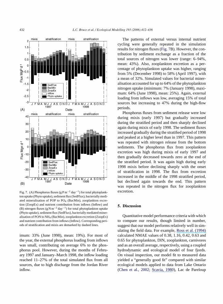
grazing of phytoplankton by zooplankton; (3) grazingof POC by zooplankton; (4) contributions of excretionand mortality of phytoplankton to the POC pool; (5)contributions of egestion and mortality of zooplanktonto the POC pool. The fluxes were calculated dailyas a volumetrically integrated value over each ofthe DYRESM layers, and then averaged monthly.In Fig. 6, the primary productivity is expressed as

a positive flux as it represents a source of carbonto the lake, while the other fluxes are expressed asnegative, representing internal cycling of carbon(not sinks). Over the 24-month simulation periodgrazing of phytoplankton by zooplankton represented4–105% of the monthly carbon assimilated in primaryproductivity (mean: 54%, S.D.: 30%) (Fig. 6). Whilegrazing of POC was low (mean: 1%, S.D.: 2%)

L.C. Bruce et al. / Ecological Modelling 193 (2006) 412–436 431

Fig. 5. Carbon biomass for field (A) and simulated (B) data andpercentage of total biomass for field (C) and simulated (D) datapresented as monthly averages for zooplankton, phytoplankton anddetrital material.

during most of the year, the contribution increasedsignificantly (9%) during the 1998Peridinium bloom,when the contribution of phytoplankton to the detritalPOC pool was also maximal. The simulated flux ofcarbon from phytoplankton and zooplankton to thePOC pool ranged from 12 to 93% (mean: 34%) andfrom 1 to 23% (mean: 9%), respectively, of the carbonassimilated in primary productivity.

4.4. Nutrient dynamics

Four major phosphorus and nitrogen fluxes to andfrom the dissolved nutrient pools were extracted from

Fig. 6. Carbon fluxes (g C m−2 day−1) for total primary productiv-ity (Total Prod), grazing of phytoplankton (Phy2Zoop) and POC(POC2Zoop) by zooplankton and egestion and mortality of phyto-plankton (Phy2POC) and zooplankton (Zoop2POC) to the POC pool.Corresponding periods of stratification and mixis are demarked bydashed lines.

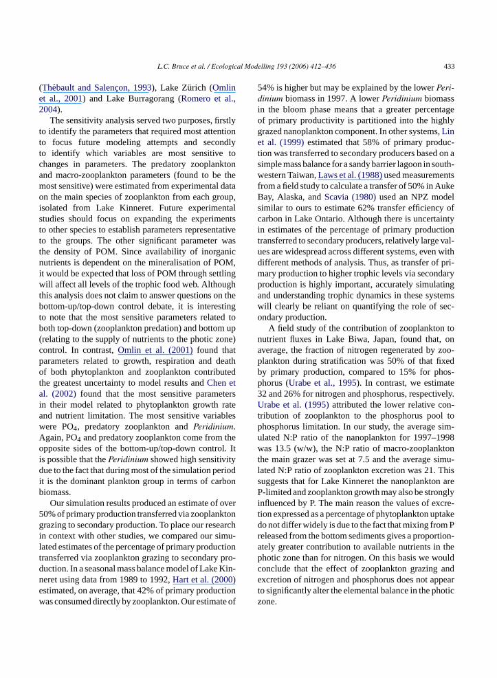
the model in order to derive the contribution of zoo-plankton to the nutrient cycles of Lake Kinneret. Thesefluxes are shown inFig. 7 and include: (1) phyto-plankton uptake; (2) sediment–water exchange; (3)bacterially mediated mineralisation; (4) zooplanktonexcretion. A fifth component, external nutrient load-ing from inflows (5) (including dissolved inorganicand particulate species), was estimated from mea-sured daily inflow volumes and nutrient concentrations.The fluxes are expressed as nutrient mass flux perday with respect to the whole lake. A negative flux(sink) represents loss of dissolved nutrients from thewater column (e.g. phytoplankton uptake) and a pos-itive flux (source) represents a gain (e.g. zooplanktonexcretion). The results, inFig. 7A, show that althoughsediment exchange makes the greatest contribution tolake-wide phosphorus fluxes (range: 22–84%, mean:54%), recycling via zooplankton excretion and bac-terially mediated mineralisation also make significantcontributions. Zooplankton excretion accounted for upto 46% of the phosphorus assimilated by phytoplankton(minimum: 3% (June 1998), maximum: 46% (August1998), mean: 26%) and simulated values for bacterialmineralisation account for up to 33% of the phyto-plankton demand (minimum: 4% (January 1998), max-

432 L.C. Bruce et al. / Ecological Modelling 193 (2006) 412–436

Fig. 7. (A) Phosphorus fluxes (g P m−2 day−1) for total phytoplank-ton uptake (Phyto uptake), sediment flux (SedFlux), bacterially medi-ated mineralisation of POP to PO4 (BacMin), zooplankton excre-tion (ZoopEx) and nutrient contribution from inflows (Inflow) and(B) nitrogen fluxes (g N m−2 day−1) for total phytoplankton uptake(Phyto uptake), sediment flux (SedFlux), bacterially mediated miner-alisation of PON to NH4 (BacMin), zooplankton excretion (ZoopEx)and nutrient contribution from inflows (Inflow). Corresponding peri-ods of stratification and mixis are demarked by dashed lines.

imum: 33% (June 1998), mean: 19%). For most ofthe year, the external phosphorus loading from inflowswas small, contributing on average 6% to the phos-phorus pool. However, during the months of Febru-ary 1997 and January–March 1998, the inflow loadingreached 11–27% of the total simulated flux from allsources, due to high discharge from the Jordan Riverinflow.

The patterns of external versus internal nutrientcycling were generally repeated in the simulationresults for nitrogen fluxes (Fig. 7B). However, the con-tribution by sediment exchange as a fraction of thetotal sources of nitrogen was lower (range: 6–94%,mean: 43%). Also, zooplankton excretion as a per-centage of phytoplankton uptake was higher, rangingfrom 5% (December 1998) to 58% (April 1997), witha mean of 32%. Simulated values for bacterial miner-alisation accounted for up to 64% of the phytoplanktonnitrogen uptake (minimum: 7% (January 1998), maxi-mum: 64% (June 1998), mean: 25%). Again, externalloading from inflows was low, averaging 15% of totalsources but increasing to 47% during the high-flowperiods.

Phosphorus fluxes from sediment release were lowduring mixis (early 1997) but gradually increasedduring the stratified period and then sharply declinedagain during mixis of early 1998. The sediment fluxesincreased gradually during the stratified period of 1998and peaked at a higher level than in 1997. This patternwas repeated with nitrogen release from the bottomsediments. The phosphorus flux from zooplanktonexcretion was high during mixis of early 1997 andthen gradually decreased towards zero at the end ofthe stratified period. It was again high during early1998 mixis before declining sharply with the onsetof stratification in 1998. The flux from excretionincreased in the middle of the 1998 stratified period,but declined again towards the end. This patternw tone

5

icht er,s im-u )c and0 resa upledh ds.O atay lare ario( p

as repeated in the nitrogen flux for zooplankxcretion.

. Discussion

Quantitative model performance criteria with who compare our results, though limited in numbuggest that our model performs relatively well in slating the field data. For example,Ross et al. (1994alculated NMAE values of 0.38, 1.16, 0.42, 0.63.65 for phytoplankton, DIN, zooplankton, carnivond as an overall average, respectively, using a coydrodynamic and ecological model of four fjorn visual inspection, our model fit to measured d

ielded a “generally good fit” compared with simicological models applied to data from Lake OntChen et al., 2002; Scavia, 1980), Lac de Parelou

L.C. Bruce et al. / Ecological Modelling 193 (2006) 412–436 433

(Thebault and Salenc¸on, 1993), Lake Zurich (Omlinet al., 2001) and Lake Burragorang (Romero et al.,2004).

The sensitivity analysis served two purposes, firstlyto identify the parameters that required most attentionto focus future modeling attempts and secondlyto identify which variables are most sensitive tochanges in parameters. The predatory zooplanktonand macro-zooplankton parameters (found to be themost sensitive) were estimated from experimental dataon the main species of zooplankton from each group,isolated from Lake Kinneret. Future experimentalstudies should focus on expanding the experimentsto other species to establish parameters representativeto the groups. The other significant parameter wasthe density of POM. Since availability of inorganicnutrients is dependent on the mineralisation of POM,it would be expected that loss of POM through settlingwill affect all levels of the trophic food web. Althoughthis analysis does not claim to answer questions on thebottom-up/top-down control debate, it is interestingto note that the most sensitive parameters related toboth top-down (zooplankton predation) and bottom up(relating to the supply of nutrients to the photic zone)control. In contrast,Omlin et al. (2001)found thatparameters related to growth, respiration and deathof both phytoplankton and zooplankton contributedthe greatest uncertainty to model results andChen etal. (2002) found that the most sensitive parametersin their model related to phytoplankton growth ratea leswA theo l. Iti yd riodi onb

over5 tong archi mu-l tiont pro-d Kin-n )e tionw te of

54% is higher but may be explained by the lowerPeri-dinium biomass in 1997. A lowerPeridinium biomassin the bloom phase means that a greater percentageof primary productivity is partitioned into the highlygrazed nanoplankton component. In other systems,Linet al. (1999)estimated that 58% of primary produc-tion was transferred to secondary producers based on asimple mass balance for a sandy barrier lagoon in south-western Taiwan,Laws et al. (1988)used measurementsfrom a field study to calculate a transfer of 50% in AukeBay, Alaska, andScavia (1980)used an NPZ modelsimilar to ours to estimate 62% transfer efficiency ofcarbon in Lake Ontario. Although there is uncertaintyin estimates of the percentage of primary productiontransferred to secondary producers, relatively large val-ues are widespread across different systems, even withdifferent methods of analysis. Thus, as transfer of pri-mary production to higher trophic levels via secondaryproduction is highly important, accurately simulatingand understanding trophic dynamics in these systemswill clearly be reliant on quantifying the role of sec-ondary production.

A field study of the contribution of zooplankton tonutrient fluxes in Lake Biwa, Japan, found that, onaverage, the fraction of nitrogen regenerated by zoo-plankton during stratification was 50% of that fixedby primary production, compared to 15% for phos-phorus (Urabe et al., 1995). In contrast, we estimate32 and 26% for nitrogen and phosphorus, respectively.Urabe et al. (1995)attributed the lower relative con-t l top im-u 998w tont imu-l hiss areP glyi cre-t ptaked Pr tion-a thep uldc ande peart oticz

nd nutrient limitation. The most sensitive variabere PO4, predatory zooplankton andPeridinium.gain, PO4 and predatory zooplankton come frompposite sides of the bottom-up/top-down contro

s possible that thePeridinium showed high sensitivitue to the fact that during most of the simulation pe

t is the dominant plankton group in terms of carbiomass.

Our simulation results produced an estimate of0% of primary production transferred via zooplankrazing to secondary production. To place our rese

n context with other studies, we compared our siated estimates of the percentage of primary producransferred via zooplankton grazing to secondaryuction. In a seasonal mass balance model of Lakeeret using data from 1989 to 1992,Hart et al. (2000stimated, on average, that 42% of primary producas consumed directly by zooplankton. Our estima

ribution of zooplankton to the phosphorus poohosphorus limitation. In our study, the average slated N:P ratio of the nanoplankton for 1997–1as 13.5 (w/w), the N:P ratio of macro-zooplank

he main grazer was set at 7.5 and the average sated N:P ratio of zooplankton excretion was 21. Tuggests that for Lake Kinneret the nanoplankton-limited and zooplankton growth may also be stron

nfluenced by P. The main reason the values of exion expressed as a percentage of phytoplankton uo not differ widely is due to the fact that mixing fromeleased from the bottom sediments gives a proportely greater contribution to available nutrients inhotic zone than for nitrogen. On this basis we woonclude that the effect of zooplankton grazingxcretion of nitrogen and phosphorus does not apo significantly alter the elemental balance in the phone.

434 L.C. Bruce et al. / Ecological Modelling 193 (2006) 412–436

6. Conclusion

The model used here was shown to reproduce theseasonal variation of biomass of the dominant phy-toplankton and zooplankton in Lake Kinneret. Themodel produced the best results when variability infield data was low and showed the biggest diver-gence when there was large scatter in the field data.The model results showed that even though zoo-plankton biomass at no stage exceeded more than22% of the total plankton carbon, zooplankton excre-tion of dissolved nutrients can account for up to 52and 48% of the phytoplankton demand for phos-phorus and nitrogen, respectively. Using the modeloutput, we were able to compare the hydrodynamicand ecological sources and sinks of nutrients in thephotic zone to determine which integrating factorsultimately determine seasonal patterns in planktonecology. The ability of numerical models, such asthe one used in this study, to couple ecological andphysical variables enables researchers to ask ques-tions that relate to the integration of both biotic andabiotic factors in limnological nutrient cycles. Fur-ther improvements to the current model formulationwill enable us to extend the ecosystem focus to ques-tions such as the role of micro-zooplankton in nutrientrecycling.

Acknowledgements

forp ter-s te-o eliW o-l iN id-i i forh Con-t arch( p-p theI tedj r-t try)s mentC

References

Alewell, C., Manderscheid, B., 1998. Use of objective criteria for theassessment of biogeochemical ecosystem models. Ecol. Model.107, 213–224.

Andersen, T., Hessen, D.O., 1991. Carbon, nitrogen, and phospho-rus content of freshwater zooplankton. Limnol. Oceanogr. 36,807–814.

Blumenshine, S.C., Hambright, K.D., 2003. Top-down control inpelagic systems: a role for invertebrate predation. Hydrobiologia491, 347–356.

Carlotti, F., Gunther, R., 1996. Seasonal dynamics of phytoplanktonandCalanus finmarchicus in the North Sea as revealed by a cou-pled one-dimensional model. Limnol. Oceanogr. 41, 522–539.

Carpenter, S.R., Kitchell, J.F., 1993. Simulation models of the trophiccascade: predictions and evaluations. In: Kitchell, S.C.J. (Ed.),The Trophic Cascade in Lakes. Cambridge University Press.

Chen, C., et al., 2002. A model study of the coupled biologicaland physical dynamics of Lake Michigan. Ecol. Model. 152,145–168.

Cole, J.F., Jones, R.C., 2000. Effect of temperature onphotosynthesis–light response and growth of four phytoplank-ton species isolated from a tidal freshwater river. J. Phycol. 36,7–16.

Cole, J.J., Carpenter, S.R., Kitchell, J.F., Pace, M.L., 2002. Pathwaysof organic carbon utilization in small lakes: results from a whole-lake 13C addition and coupled model. Limnol. Oceanogr. 47,1664–1675.

Easton, J., Gophen, M., 2003. Diel variation in the vertical distri-bution of fish and plankton in Lake Kinneret: a 24-h study ofecological overlap. Hydrobiologia 491, 91–100.

Gal, G., Imberger, J., Zohary, T., Antenucci, J.P., Anis, A., Rosenberg,T., 2003. Simulating the thermal dynamics of Lake Kinneret.Ecol. Model. 162, 69–86.

Gilbert, P.M., 1998. Interactions of top-down and bottom-up control

G mmo-

G anda

G nage-.

G ktonol.

G hedur-tern

H al dis-ake

H ndakes.

The authors thank the following organisationsroviding the data used in this study: Mekorot Wahed Unit, Israel Hydrological Services, Israel Merological Services, the Kinneret Authority, Israater Commission (IWC) and the Kinneret Limn

ogical Laboratory (KLL). We particularly thank Amishri, Yossi Yacobi and Arkadi Parparov for prov

ng unpublished data and advice, Anas Ghadouanis valuable comments on the manuscript and the

ract Research Group at the Centre for Water ReseCWR), in particular David Horn, for technical suort for the project. Funding was provided by

WC via the Kinneret Modeling Project, conducointly by KLL and CWR. The first author was fuher funded by an Australian Postgraduate (Induscholarship, sponsored by the Wheatbelt Developommission.

in planktonic nitrogen cycling. Hydrobiologia 363, 1–12.ophen, M., 1976a. Temperature dependence of food intake, a

nia excretion and respiration inCeriodaphnia reticulata (Jurine)(Lake Kinneret, Israel). Freshwater Biol. 6, 451–455.

ophen, M., 1976b. Temperature effect on lifespan, metabolismdevelopment time ofMesocyclops leuckarti (Claus). Oceologi25, 271–277.

ophen, M., 1984. The impact of zooplankton status on the mament of Lake Kinneret (Israel). Hydrobiologia 113, 249–258

ophen, M., Azoulay, B., 2002. The trophic status of zooplancommunities in Lake Kinneret (Israel). Verh. Int. Ver. Limn28, 836–839.

riffin, S.L., Herzfeld, M., Hamilton, D.P., 2000. Modelling timpact of zooplankton grazing on phytoplankton biomassing a dinoflagellate bloom in the Swan River estuary, WesAustralia. Ecol. Eng. 16, 373–394.

adas, O., Berman, T., 1998. Seasonal abundance and vertictribution of protozoa (flagellates, ciliates) and bacteria in LKinneret, Israel. Aquat. Microbiol. 14, 161–170.

akanson, L., Boulion, V.V., 2003. Modelling production abiomasses of herbivorous and predatory zooplankton in lEcol. Model. 161, 1–33.

L.C. Bruce et al. / Ecological Modelling 193 (2006) 412–436 435

Hambright, K.D., Gophen, M., Serruya, S., 1994. Influence of long-term climatic changes on the stratification of a subtropical, warmmonomictic lake. Limnol. Oceanogr. 39, 1233–1242.

Haney, J.F., Trout, M.A., 1985. Selective grazing by zooplankton inLake Titicaca. Ergeb. Limnol. 21, 147–160.

Hart, D.R., Stone, L., Berman, T., 2000. Seasonal dynamics of theLake Kinneret food web: the importance of the microbial loop.Limnol. Oceanogr. 45, 350–361.

Hongping, P., Jianyi, M., 2002. Study on the algal dynamic modelfor West Lake Hangzhou. Ecol. Model. 148, 67–77.

Hudson, J.J., Taylor, W.D., 1996. Measuring regeneration ofdissolved phosphorus in planktonic communities. Limnol.Oceanogr. 41, 1560–1565.

Hudson, J.J., Taylor, W.D., Schindler, D.W., 1999. Planktonic nutri-ent regeneration and cycling efficiency in temperate lakes. Nature400, 659–661.

Ji, R., et al., 2005. Influences of suspended sediments on the ecosys-tem in Lake Michigan: a 3-D coupled bio-physical modelingexperiment. Ecol. Model. 152, 169–190.

Jewson, D.H., 1977. Light penetration in relation to phytoplanktoncontent of the eutrophic zone of Lough Neagh, N. Ireland. Oikos28, 74–83.

Jorgensen, S.E., Bendoricchio, G., 2001. Fundamentals of EcologicalModeling, third ed. Elsevier.

Kirk, J.T.O., 1994. Light and Photosynthesis in Aquatic Ecosystems,second ed. Cambridge Press.

Krivtsov, V., Goldspink, C., Sigee, D.C., Bellinger, E.G., 2001.Expansion of the model ‘Rostherne’ for fish and zooplankton:role of top-down effects in modifying the prevailing pattern ofecosystem functioning. Ecol. Model. 138, 153–171.

Landry, M.R., Hassett, R.P., 1985. Time scales in behavioral, bio-chemical, and energetic adaptations to food-limiting conditionsby a marine copepod. Ergeb. Limnol. 21, 209–222.

Laws, E.A., Bienfang, P.K., Ziemann, D.A., Conquest, L.D., 1988.Phytoplankton population dynamics and the fate of production

ogr.

L lank-.

L n ati. 58,

L ra in

M ction

1.M rate

tion

O odel41,

O igat-sterndel.

Pollingher, U., 1986. Phytoplankton periodicity in a sub-tropical lake (Lake Kinneret, Israel). Hydrobiologia 138, 127–138.

Pollingher, U., Berman, T., 1982. Relative contributions of net andnano phytoplankton to primary production in Lake Kinneret(Israel). Arch. Hydrobiol. 96, 33–46.

Putt, M., Stockner, 1989. An experimentally determined car-bon:volume ratio for marine oligotrichous ciliates from estuarineand coastal waters. Limnol. Oceanogr. 34, 1097–1103.

Reynolds, C.S., 1984. The Ecology of Freshwater Phytoplankton.Cambridge Press.

Robson, B.J., Hamilton, D.P., 2004. Three-dimensional modellingof a Microcystis bloom event in the Swan River estuary, WesternAustralia. Ecol. Model. 174, 203–222.

Romero, J.R., Antenucci, J.P., Imberger, J., 2004. One- and three-dimensional biogeochemical simulations of two differing reser-voirs. Ecol. Model. 174, 143–160.

Ross, A.H., Gurney, S.C., Heath, M.R., 1994. A comparative studyof the ecosystem dynamics of four fjords. Limnol. Oceanogr. 39,318–343.

Rukhovets, L.A., Astrakhantsev, G.P., Menshutkin, V.V., Minina,T.R., Petrova, N.A., Poloskov, V.N., 2003. Development of LakeLadoga ecosystem models: modeling of the phytoplankton suc-cession in the eutrophication process. I. Ecol. Model. 165, 49–77.

Scavia, D., 1980. An ecological model of Lake Ontario. Ecol. Model.8, 49–78.

Scavia, D., Lang, G.A., Kitchell, J.F., 1988. Dynamics of Lake Michi-gan plankton: a model evaluation of nutrient loading, competitionand predation. Can. J. Fish. Aquat. Sci. 45, 165–177.

Serruya, C., 1978. Lake Kinneret. Junk.Serruya, C., Berman, T., 1976. Phosphorus, nitrogen and the growth

of algae in Lake Kinneret. J. Phycol. 11, 155–162.Serruya, C., Edelstein, M., Pollingher, U., Serruya, S., 1974.

Lake Kinneret sediments: nutrient composition of the pore489–

S d foodim-

S algal

T hiccol.

U eta-Lake

V sys-

W s and. 39,

W rela-n ofk-

during the spring bloom in Auke Bay, Alaska. Limnol. Ocean33, 57–65.

ehman, J.T., 1980. Release and cycling of nutrients between ptonic algae and herbivores. Limnol. Oceanogr. 25, 620–632

in, H.J., et al., 1999. A trophic model of a sandy barrier lagooChiku in southwestern Taiwan. Estuarine Coastal Shelf Sc575–588.

unte, C.C., Leucke, C., 1990. Trophic interactions of LeptodoLake Mendota. Limnol. Oceanogr. 35, 1091–1100.

adoni, P., Berman, T., Hadas, O., Pinkas, R., 1990. Food seleand growth of the planktonic ciliateColeps hirtus isolated froma monomictic subtropical lake. J. Plankton Res. 12, 735–74

ehner, T., 2000. Influence of spring warming on the predationof underyearling fish on Daphnia—a deterministic simulaapproach. Freshwater Biol. 45, 253–263.

mlin, M., Reichert, P., Forster, R., 2001. Biogeochemical mof Lake Zurich: model equations and results. Ecol. Model. 177–103.

sidele, O.O., Beck, M.B., 2004. Food web modelling for investing ecosystem behaviour in large reservoirs of the south-eaUnited States: lessons from Lake Lanier Georgia. Ecol. Mo173, 129–158.

water and mud water exchanges. Limnol. Oceanogr. 19,508.

temberger, R.S., Gilbert, J.J., 1985. Assessment of threshollevels and population growth in planktonic rotifers. Ergeb. Lnol. 21, 269–276.

terner, R.W., 1986. Herbivores’ direct and indirect effects onpopulations. Science 231, 605–607.

hebault, J., Salenc¸on, M., 1993. Simulation model of a mesotropreservoir (Lac de Pareloup, France): biological model. EModel. 65, 1–30.

rabe, J., Nakanishi, M., Kawabata, K., 1995. Contribution of mzoan plankton to the cycling of nitrogen and phosphorus inBiwa. Limnol. Oceanogr. 40, 232–241.

anni, M.J., 2002. Nutrient cycling by animals in freshwater ecotems. Annu. Rev. Ecol. Syst. 33, 341–370.

en, Y.H., Peters, R.H., 1994. Empirical models of phosphorunitrogen excretion rates by zooplankton. Limnol. Oceanogr1669–1679.

ynne, D., Panti, N.J., Aaronson, S., Berman, T., 1982. Thetionship between nutrient status and chemical compositioPeridinium cinctum during the bloom of Lake Kinneret. J. Planton Res. 4, 125–134.

436 L.C. Bruce et al. / Ecological Modelling 193 (2006) 412–436

Yacobi, Y.Z., Kalikhman, I., Gophen, M., Walline, P., 1993. Thespatial distribution of temperature, oxygen, plankton and fishdetermined simultaneously in Lake Kinneret, Israel. J. PlanktonRes. 15, 589–601.

Yeates, P.S., Imberger, J., 2004. Pseudo two-dimensional simulationsof internal and boundary fluxes in stratified lakes and reservoirs.Int. J. River Basin Res. 1, 1–23.

Zohary, T., 2004. Changes to the phytoplankton assemblage of LakeKinneret after decades of a predictable, repetitive pattern. Fresh-water Biol. 49, 1355–1371.

Zohary, T., Erez, J.G.M., Bernam-Frank, I., Stiller, M., 1994. Sea-sonality of stable carbon isotopes within the pelagic food web ofLake Kinneret. Limnol. Oceanogr. 39, 1030–1043.