A novel signal compression method based on optimal ensemble empirical mode decomposition for bearing vibration signals Wei Guo, Peter W. Tse n The Smart Engineering Asset Management Laboratory and the Croucher Optical Nondestructive Testing Laboratory, Department of Systems Engineering and Engineering Management, City University of Hong Kong, 83 Tat Chee Ave., Kowloon Tong, Hong Kong article info Article history: Received 5 January 2012 Received in revised form 21 August 2012 Accepted 21 August 2012 Handling Editor: K. Worden Available online 30 September 2012 abstract Today, remote machine condition monitoring is popular due to the continuous advancement in wireless communication. Bearing is the most frequently and easily failed component in many rotating machines. To accurately identify the type of bearing fault, large amounts of vibration data need to be collected. However, the volume of transmitted data cannot be too high because the bandwidth of wireless communication is limited. To solve this problem, the data are usually compressed before transmitting to a remote maintenance center. This paper proposes a novel signal compression method that can substantially reduce the amount of data that need to be transmitted without sacrificing the accuracy of fault identification. The proposed signal compression method is based on ensemble empirical mode decomposition (EEMD), which is an effective method for adaptively decomposing the vibration signal into different bands of signal components, termed intrinsic mode functions (IMFs). An optimization method was designed to automatically select appropriate EEMD parameters for the analyzed signal, and in particular to select the appropriate level of the added white noise in the EEMD method. An index termed the relative root-mean-square error was used to evaluate the decomposition performances under different noise levels to find the optimal level. After applying the optimal EEMD method to a vibration signal, the IMF relating to the bearing fault can be extracted from the original vibration signal. Compressing this signal component obtains a much smaller proportion of data samples to be retained for transmission and further reconstruction. The proposed compression method were also compared with the popular wavelet compression method. Experimental results demonstrate that the optimization of EEMD parameters can automatically find appro- priate EEMD parameters for the analyzed signals, and the IMF-based compression method provides a higher compression ratio, while retaining the bearing defect characteristics in the transmitted signals to ensure accurate bearing fault diagnosis. & 2012 Elsevier Ltd. All rights reserved. 1. Introduction In industry, remote condition monitoring systems are designed to collect data for remotely assessing the health condition of important machine elements. For example, rolling bearings are the most important elements in the vast majority of rotating machines. Serious bearing failure may cause downtime costs or significant damage to other parts of Contents lists available at SciVerse ScienceDirect journal homepage: www.elsevier.com/locate/jsvi Journal of Sound and Vibration 0022-460X/$ - see front matter & 2012 Elsevier Ltd. All rights reserved. http://dx.doi.org/10.1016/j.jsv.2012.08.017 n Corresponding author. Tel.: þ852 3442 8431; fax: þ852 3442 0415. E-mail address: [email protected] (P.W. Tse). Journal of Sound and Vibration 332 (2013) 423–441

Welcome message from author
This document is posted to help you gain knowledge. Please leave a comment to let me know what you think about it! Share it to your friends and learn new things together.
Transcript

Contents lists available at SciVerse ScienceDirect
Journal of Sound and Vibration
Journal of Sound and Vibration 332 (2013) 423–441
0022-46
http://d
n Corr
E-m
journal homepage: www.elsevier.com/locate/jsvi
A novel signal compression method based on optimal ensembleempirical mode decomposition for bearing vibration signals
Wei Guo, Peter W. Tse n
The Smart Engineering Asset Management Laboratory and the Croucher Optical Nondestructive Testing Laboratory, Department of Systems
Engineering and Engineering Management, City University of Hong Kong, 83 Tat Chee Ave., Kowloon Tong, Hong Kong
a r t i c l e i n f o
Article history:
Received 5 January 2012
Received in revised form
21 August 2012
Accepted 21 August 2012
Handling Editor: K. Wordentransmitted data cannot be too high because the bandwidth of wireless communication
Available online 30 September 2012
0X/$ - see front matter & 2012 Elsevier Ltd.
x.doi.org/10.1016/j.jsv.2012.08.017
esponding author. Tel.: þ852 3442 8431; fa
ail address: [email protected] (P.W. Tse).
a b s t r a c t
Today, remote machine condition monitoring is popular due to the continuous
advancement in wireless communication. Bearing is the most frequently and easily
failed component in many rotating machines. To accurately identify the type of bearing
fault, large amounts of vibration data need to be collected. However, the volume of
is limited. To solve this problem, the data are usually compressed before transmitting to
a remote maintenance center. This paper proposes a novel signal compression method
that can substantially reduce the amount of data that need to be transmitted without
sacrificing the accuracy of fault identification. The proposed signal compression method
is based on ensemble empirical mode decomposition (EEMD), which is an effective
method for adaptively decomposing the vibration signal into different bands of signal
components, termed intrinsic mode functions (IMFs). An optimization method was
designed to automatically select appropriate EEMD parameters for the analyzed signal,
and in particular to select the appropriate level of the added white noise in the EEMD
method. An index termed the relative root-mean-square error was used to evaluate the
decomposition performances under different noise levels to find the optimal level. After
applying the optimal EEMD method to a vibration signal, the IMF relating to the bearing
fault can be extracted from the original vibration signal. Compressing this signal
component obtains a much smaller proportion of data samples to be retained for
transmission and further reconstruction. The proposed compression method were also
compared with the popular wavelet compression method. Experimental results
demonstrate that the optimization of EEMD parameters can automatically find appro-
priate EEMD parameters for the analyzed signals, and the IMF-based compression
method provides a higher compression ratio, while retaining the bearing defect
characteristics in the transmitted signals to ensure accurate bearing fault diagnosis.
& 2012 Elsevier Ltd. All rights reserved.
1. Introduction
In industry, remote condition monitoring systems are designed to collect data for remotely assessing the healthcondition of important machine elements. For example, rolling bearings are the most important elements in the vastmajority of rotating machines. Serious bearing failure may cause downtime costs or significant damage to other parts of
All rights reserved.
x: þ852 3442 0415.
W. Guo, P.W. Tse / Journal of Sound and Vibration 332 (2013) 423–441424
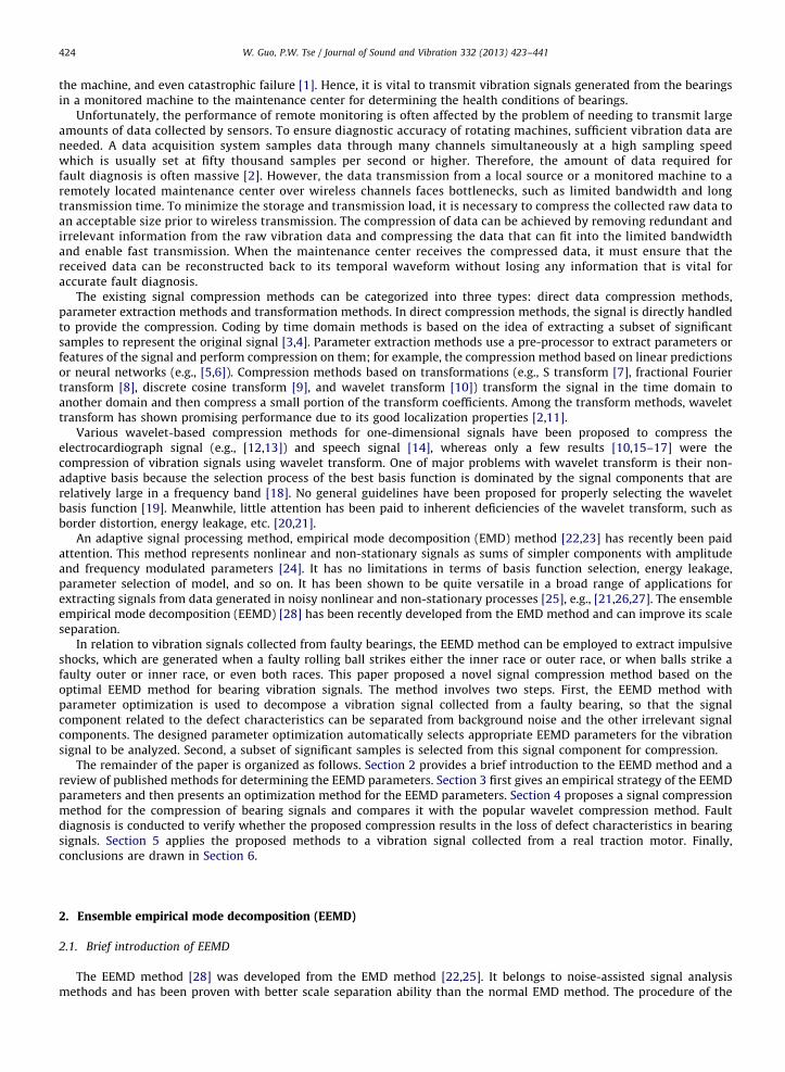
the machine, and even catastrophic failure [1]. Hence, it is vital to transmit vibration signals generated from the bearingsin a monitored machine to the maintenance center for determining the health conditions of bearings.
Unfortunately, the performance of remote monitoring is often affected by the problem of needing to transmit largeamounts of data collected by sensors. To ensure diagnostic accuracy of rotating machines, sufficient vibration data areneeded. A data acquisition system samples data through many channels simultaneously at a high sampling speedwhich is usually set at fifty thousand samples per second or higher. Therefore, the amount of data required forfault diagnosis is often massive [2]. However, the data transmission from a local source or a monitored machine to aremotely located maintenance center over wireless channels faces bottlenecks, such as limited bandwidth and longtransmission time. To minimize the storage and transmission load, it is necessary to compress the collected raw data toan acceptable size prior to wireless transmission. The compression of data can be achieved by removing redundant andirrelevant information from the raw vibration data and compressing the data that can fit into the limited bandwidthand enable fast transmission. When the maintenance center receives the compressed data, it must ensure that thereceived data can be reconstructed back to its temporal waveform without losing any information that is vital foraccurate fault diagnosis.
The existing signal compression methods can be categorized into three types: direct data compression methods,parameter extraction methods and transformation methods. In direct compression methods, the signal is directly handledto provide the compression. Coding by time domain methods is based on the idea of extracting a subset of significantsamples to represent the original signal [3,4]. Parameter extraction methods use a pre-processor to extract parameters orfeatures of the signal and perform compression on them; for example, the compression method based on linear predictionsor neural networks (e.g., [5,6]). Compression methods based on transformations (e.g., S transform [7], fractional Fouriertransform [8], discrete cosine transform [9], and wavelet transform [10]) transform the signal in the time domain toanother domain and then compress a small portion of the transform coefficients. Among the transform methods, wavelettransform has shown promising performance due to its good localization properties [2,11].
Various wavelet-based compression methods for one-dimensional signals have been proposed to compress theelectrocardiograph signal (e.g., [12,13]) and speech signal [14], whereas only a few results [10,15–17] were thecompression of vibration signals using wavelet transform. One of major problems with wavelet transform is their non-adaptive basis because the selection process of the best basis function is dominated by the signal components that arerelatively large in a frequency band [18]. No general guidelines have been proposed for properly selecting the waveletbasis function [19]. Meanwhile, little attention has been paid to inherent deficiencies of the wavelet transform, such asborder distortion, energy leakage, etc. [20,21].
An adaptive signal processing method, empirical mode decomposition (EMD) method [22,23] has recently been paidattention. This method represents nonlinear and non-stationary signals as sums of simpler components with amplitudeand frequency modulated parameters [24]. It has no limitations in terms of basis function selection, energy leakage,parameter selection of model, and so on. It has been shown to be quite versatile in a broad range of applications forextracting signals from data generated in noisy nonlinear and non-stationary processes [25], e.g., [21,26,27]. The ensembleempirical mode decomposition (EEMD) [28] has been recently developed from the EMD method and can improve its scaleseparation.
In relation to vibration signals collected from faulty bearings, the EEMD method can be employed to extract impulsiveshocks, which are generated when a faulty rolling ball strikes either the inner race or outer race, or when balls strike afaulty outer or inner race, or even both races. This paper proposed a novel signal compression method based on theoptimal EEMD method for bearing vibration signals. The method involves two steps. First, the EEMD method withparameter optimization is used to decompose a vibration signal collected from a faulty bearing, so that the signalcomponent related to the defect characteristics can be separated from background noise and the other irrelevant signalcomponents. The designed parameter optimization automatically selects appropriate EEMD parameters for the vibrationsignal to be analyzed. Second, a subset of significant samples is selected from this signal component for compression.
The remainder of the paper is organized as follows. Section 2 provides a brief introduction to the EEMD method and areview of published methods for determining the EEMD parameters. Section 3 first gives an empirical strategy of the EEMDparameters and then presents an optimization method for the EEMD parameters. Section 4 proposes a signal compressionmethod for the compression of bearing signals and compares it with the popular wavelet compression method. Faultdiagnosis is conducted to verify whether the proposed compression results in the loss of defect characteristics in bearingsignals. Section 5 applies the proposed methods to a vibration signal collected from a real traction motor. Finally,conclusions are drawn in Section 6.
2. Ensemble empirical mode decomposition (EEMD)
2.1. Brief introduction of EEMD
The EEMD method [28] was developed from the EMD method [22,25]. It belongs to noise-assisted signal analysismethods and has been proven with better scale separation ability than the normal EMD method. The procedure of the

W. Guo, P.W. Tse / Journal of Sound and Vibration 332 (2013) 423–441 425
EEMD method can be briefly summarized as follows:
Step 1:Add white noise with a predefined noise amplitude to the signal to be analyzed.Step 2:Use the EMD method to decompose the newly generated signal.Step 3:Repeat the above signal decomposition with different white noise, in which the amplitude of the added whitenoise is fixed.Step 4:Calculate the ensemble means of the decomposition results as final results.
Using this signal processing method, a multi-component signal, x(k), is decomposed into a finite number of intrinsicmode functions (IMFs) and a residue,
xðkÞ ¼Xn
i ¼ 1
ciþr, (1)
where n represents the number of the IMFs, ci is the ith IMF that is the ensemble mean of the corresponding IMFs obtainedfrom all of decomposition processes, and r is the mean of the residues from all of decomposition processes.
In each decomposition process, the added white noise helps to perturb the analyzed signal and enables the EMD method tovisit all possible solutions in the finite neighborhood of the true final IMF [28]. Based on the property of zero mean of white noise,the added white noise can be cancelled out in the final ensemble mean if there are sufficient trials. Only the signal itself cansurvive in the final decomposition results. For more details about the EMD and the EEMD methods, please refer to Refs. [22,25,28].
2.2. Review of EEMD parameter selection
In the EEMD method, two critical parameters, the amplitude of the added white noise, AN, and the ensemble number,NE, need to be prescribed. The previous research about the method for selecting EEMD parameters can be summarized intothe following points:
First, the problem of the automatic selection of EEMD parameters is still unsolved and required further investigation.The amplitude of the added white noise was proven to be chosen appropriately for good performance of the EEMD method.Lei et al. [29–31] and Zhou et al. [32] convinced that there were no specific equations reported in the literature to guide thechoice of EEMD parameters, especially the noise amplitude. Developing methods for automatically selecting the EEMDparameters aiming at different signals are thus needed in future research [29–31].
Second, the EEMD method was applied and developed for processing various signals, in which the EEMD parameterswere set using trial and error or empirical values. Lei et al. [29–31] tried different noise amplitudes and selected fromthem. In most of cases (e.g., [33,34]), the noise amplitude was set to the empirical value suggested by Wu and Huang [28]or the authors’ empirical value without providing detailed explanations. Wu et al. [35] proposed an improved EEMDmethod without mentioning how to automatically select the appropriate EEMD parameters.
Third, Zvokelj et al. [36,37], Chang and Liu [38], Zhang et al. [39], and Yeh et al. [40] independently introduced thesignal-to-noise ratio (SNR) as a performance index to select the noise amplitude. The assumption of their methods is theanalyzed signal or its power is known a priori. For real vibration signals, Zvokelj et al. [36,37] still used the empiricalsetting as proposed by Wu and Huang [28].
Niazy et al. [41] used relative root-mean-square error (RMSE) to evaluate the performances of EEMD when tryingdifferent levels of the added white noise, however, they did not give any guidance on how to select the appropriate noiselevel based on the relative RMSE. Having analyzed the characteristics of bearing vibration signals, an optimization methodwas designed to automatically select EEMD parameters for the target vibration signal.
3. Optimization for EEMD parameters
3.1. Observations on parameter setting
Wu and Huang [28] described the effect of the added white noise and these two parameters satisfy the followingequation that
ln eþAN
2� lnNE ¼ 0, (2)
where e represents the standard deviation of error between the original signal and the corresponding IMF(s). The empiricalsetting is as follows: the amplitude of the added white noise is approximately 0.2 of a standard deviation of the original signaland the value of the ensemble is a few hundreds. This is not always usable for signal processing in different applications.
Following many simulations and experiments, an empirical strategy has been devised for determining the EEMDparameters [42].
(1)
The noise amplitude greatly influences the performance of the EEMD method with regard to scale separation. Once thenoise amplitude is determined, increasing the ensemble number is helpful for reducing the remaining noise in each IMF.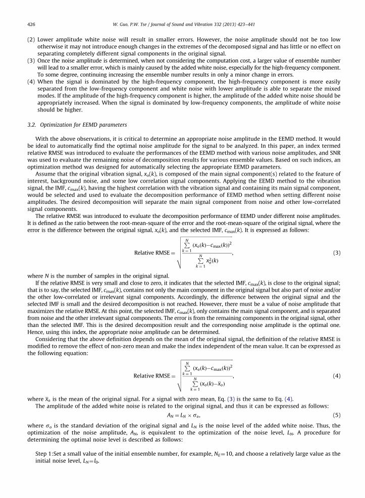
W. Guo, P.W. Tse / Journal of Sound and Vibration 332 (2013) 423–441426
(2)
Lower amplitude white noise will result in smaller errors. However, the noise amplitude should not be too lowotherwise it may not introduce enough changes in the extremes of the decomposed signal and has little or no effect onseparating completely different signal components in the original signal.(3)
Once the noise amplitude is determined, when not considering the computation cost, a larger value of ensemble numberwill lead to a smaller error, which is mainly caused by the added white noise, especially for the high-frequency component.To some degree, continuing increasing the ensemble number results in only a minor change in errors.(4)
When the signal is dominated by the high-frequency component, the high-frequency component is more easilyseparated from the low-frequency component and white noise with lower amplitude is able to separate the mixedmodes. If the amplitude of the high-frequency component is higher, the amplitude of the added white noise should beappropriately increased. When the signal is dominated by low-frequency components, the amplitude of white noiseshould be higher.3.2. Optimization for EEMD parameters
With the above observations, it is critical to determine an appropriate noise amplitude in the EEMD method. It wouldbe ideal to automatically find the optimal noise amplitude for the signal to be analyzed. In this paper, an index termedrelative RMSE was introduced to evaluate the performances of the EEMD method with various noise amplitudes, and SNRwas used to evaluate the remaining noise of decomposition results for various ensemble values. Based on such indices, anoptimization method was designed for automatically selecting the appropriate EEMD parameters.
Assume that the original vibration signal, xo(k), is composed of the main signal component(s) related to the feature ofinterest, background noise, and some low correlation signal components. Applying the EEMD method to the vibrationsignal, the IMF, cmax(k), having the highest correlation with the vibration signal and containing its main signal component,would be selected and used to evaluate the decomposition performance of EEMD method when setting different noiseamplitudes. The desired decomposition will separate the main signal component from noise and other low-correlatedsignal components.
The relative RMSE was introduced to evaluate the decomposition performance of EEMD under different noise amplitudes.It is defined as the ratio between the root-mean-square of the error and the root-mean-square of the original signal, where theerror is the difference between the original signal, xo(k), and the selected IMF, cmax(k). It is expressed as follows:
Relative RMSE¼
ffiffiffiffiffiffiffiffiffiffiffiffiffiffiffiffiffiffiffiffiffiffiffiffiffiffiffiffiffiffiffiffiffiffiffiffiffiffiffiffiffiffiffiffiPN
k ¼ 1
ðxoðkÞ�cmaxðkÞÞ2
PNk ¼ 1
x2o ðkÞ
vuuuuuut , (3)
where N is the number of samples in the original signal.If the relative RMSE is very small and close to zero, it indicates that the selected IMF, cmax(k), is close to the original signal;
that is to say, the selected IMF, cmax(k), contains not only the main component in the original signal but also part of noise and/orthe other low-correlated or irrelevant signal components. Accordingly, the difference between the original signal and theselected IMF is small and the desired decomposition is not reached. However, there must be a value of noise amplitude thatmaximizes the relative RMSE. At this point, the selected IMF, cmax(k), only contains the main signal component, and is separatedfrom noise and the other irrelevant signal components. The error is from the remaining components in the original signal, otherthan the selected IMF. This is the desired decomposition result and the corresponding noise amplitude is the optimal one.Hence, using this index, the appropriate noise amplitude can be determined.
Considering that the above definition depends on the mean of the original signal, the definition of the relative RMSE ismodified to remove the effect of non-zero mean and make the index independent of the mean value. It can be expressed asthe following equation:
Relative RMSE¼
ffiffiffiffiffiffiffiffiffiffiffiffiffiffiffiffiffiffiffiffiffiffiffiffiffiffiffiffiffiffiffiffiffiffiffiffiffiffiffiffiffiffiffiffiPN
k ¼ 1
ðxoðkÞ�cmaxðkÞÞ2
PNk ¼ 1
ðxoðkÞ�xoÞ
vuuuuuut , (4)
where xo is the mean of the original signal. For a signal with zero mean, Eq. (3) is the same to Eq. (4).The amplitude of the added white noise is related to the original signal, and thus it can be expressed as follows:
AN ¼ LN � so, (5)
where so is the standard deviation of the original signal and LN is the noise level of the added white noise. Thus, theoptimization of the noise amplitude, AN, is equivalent to the optimization of the noise level, LN. A procedure fordetermining the optimal noise level is described as follows:
Step 1:Set a small value of the initial ensemble number, for example, NE¼10, and choose a relatively large value as theinitial noise level, LN¼ l0.
W. Guo, P.W. Tse / Journal of Sound and Vibration 332 (2013) 423–441 427
Step 2:Perform the signal decomposition using the EEMD method and calculate the relative RMSE. It is unnecessary toextract all of the IMFs to find the optimal noise level, as only the IMF with the largest correlation coefficient relative tothe signal is used to calculate the relative RMSE. During the process of signal decomposition, when the correlationcoefficient of the current IMF is sufficiently small, the decomposition stops.Step 3:Decrease the noise level, LN, and retain the initial ensemble number for the next decomposition. Repeat step 2until the change in the relative RMSE is negligible.Step 4:The optimal noise level is the value that maximizes the relative RMSE, where the maximal relative RMSE isarrived at by determining the maximum numerically.
Once the optimal noise level is determined, the remaining task is to choose an appropriate value for the ensemblenumber. Too large a value of ensemble number will lead to a higher computation cost. Too small a value will not be enoughto cancel out the noise remaining in each IMF. Here, the widely accepted and used measure, the signal-to-noise ratio (SNR),was introduced to determine the appropriate ensemble number. The procedure is to fix the optimal noise level andincrease the ensemble number until the change in the SNR value is relatively small. The following section used variousvibration signals to illustrate the proposed optimization method and verify its effectiveness.
3.3. Experiments-vibration signal decomposition
Two vibration signals were collected from faulty bearings and then decomposed using the optimal EEMD method. Thisis also pre-processing for further signal compression.
3.3.1. The rationale for experiment setup
To verify the proposed methods on the effectiveness for remote bearing monitoring, two types of experiments were setup. The first type of experiments was performed in a controlled environment, such as a laboratory using a smaller electricmotor running with a bearing. The intention of such experiments is to ensure that the desired tests can be conductedsuccessfully on a smaller motor before performing real tests on expensive traction motors used in real trains. The secondtype of experiments was conducted using a real and expensive traction motor, which would be described in Section 5.
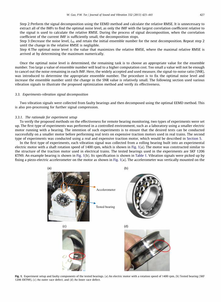
In the first type of experiments, each vibration signal was collected from a rolling bearing built into an experimentalelectric motor with a shaft rotation speed of 1400 rpm, which is shown in Fig. 1(a). The motor was constructed similar tothe structure of the traction motor used in electrical trains. The tested bearings used in the experiments are SKF 1206KTN9. An example bearing is shown in Fig. 1(b). Its specification is shown in Table 1. Vibration signals were picked up byfixing a piezo-electric accelerometer on the motor as shown in Fig. 1(a). The accelerometer was vertically mounted on the
Accelerometer
Tested bearing
Fig. 1. Experiment setup and faulty components of the tested bearings. (a) An electric motor with a rotation speed of 1400 rpm, (b) Tested bearing (SKF
1206 EKTN9), (c) An outer race defect, and (d) An Inner race defect.
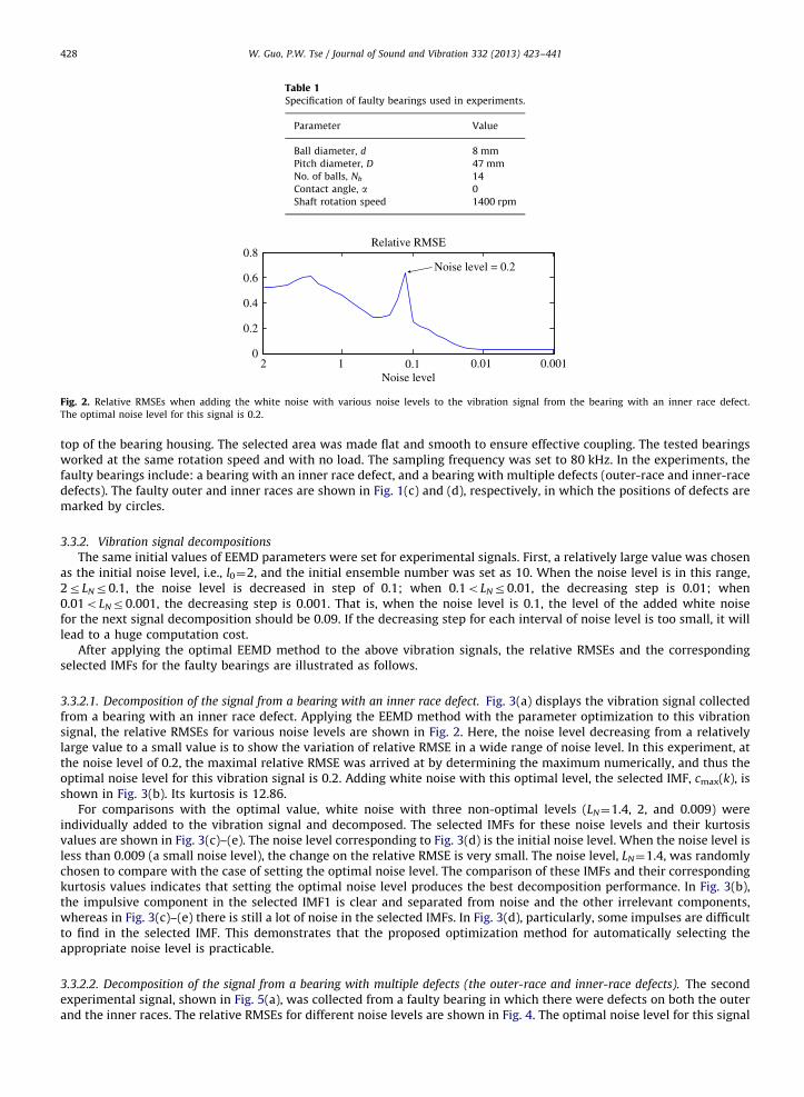
Table 1Specification of faulty bearings used in experiments.
Parameter Value
Ball diameter, d 8 mm
Pitch diameter, D 47 mm
No. of balls, Nb 14
Contact angle, a 0
Shaft rotation speed 1400 rpm
0
0.2
0.4
0.6
0.8Relative RMSE
2 1 0.1 0.01 0.001Noise level
Noise level = 0.2
Fig. 2. Relative RMSEs when adding the white noise with various noise levels to the vibration signal from the bearing with an inner race defect.
The optimal noise level for this signal is 0.2.
W. Guo, P.W. Tse / Journal of Sound and Vibration 332 (2013) 423–441428
top of the bearing housing. The selected area was made flat and smooth to ensure effective coupling. The tested bearingsworked at the same rotation speed and with no load. The sampling frequency was set to 80 kHz. In the experiments, thefaulty bearings include: a bearing with an inner race defect, and a bearing with multiple defects (outer-race and inner-racedefects). The faulty outer and inner races are shown in Fig. 1(c) and (d), respectively, in which the positions of defects aremarked by circles.
3.3.2. Vibration signal decompositions
The same initial values of EEMD parameters were set for experimental signals. First, a relatively large value was chosenas the initial noise level, i.e., l0¼2, and the initial ensemble number was set as 10. When the noise level is in this range,2rLNr0.1, the noise level is decreased in step of 0.1; when 0.1oLNr0.01, the decreasing step is 0.01; when0.01oLNr0.001, the decreasing step is 0.001. That is, when the noise level is 0.1, the level of the added white noisefor the next signal decomposition should be 0.09. If the decreasing step for each interval of noise level is too small, it willlead to a huge computation cost.
After applying the optimal EEMD method to the above vibration signals, the relative RMSEs and the correspondingselected IMFs for the faulty bearings are illustrated as follows.
3.3.2.1. Decomposition of the signal from a bearing with an inner race defect. Fig. 3(a) displays the vibration signal collectedfrom a bearing with an inner race defect. Applying the EEMD method with the parameter optimization to this vibrationsignal, the relative RMSEs for various noise levels are shown in Fig. 2. Here, the noise level decreasing from a relativelylarge value to a small value is to show the variation of relative RMSE in a wide range of noise level. In this experiment, atthe noise level of 0.2, the maximal relative RMSE was arrived at by determining the maximum numerically, and thus theoptimal noise level for this vibration signal is 0.2. Adding white noise with this optimal level, the selected IMF, cmax(k), isshown in Fig. 3(b). Its kurtosis is 12.86.
For comparisons with the optimal value, white noise with three non-optimal levels (LN¼1.4, 2, and 0.009) wereindividually added to the vibration signal and decomposed. The selected IMFs for these noise levels and their kurtosisvalues are shown in Fig. 3(c)–(e). The noise level corresponding to Fig. 3(d) is the initial noise level. When the noise level isless than 0.009 (a small noise level), the change on the relative RMSE is very small. The noise level, LN¼1.4, was randomlychosen to compare with the case of setting the optimal noise level. The comparison of these IMFs and their correspondingkurtosis values indicates that setting the optimal noise level produces the best decomposition performance. In Fig. 3(b),the impulsive component in the selected IMF1 is clear and separated from noise and the other irrelevant components,whereas in Fig. 3(c)–(e) there is still a lot of noise in the selected IMFs. In Fig. 3(d), particularly, some impulses are difficultto find in the selected IMF. This demonstrates that the proposed optimization method for automatically selecting theappropriate noise level is practicable.
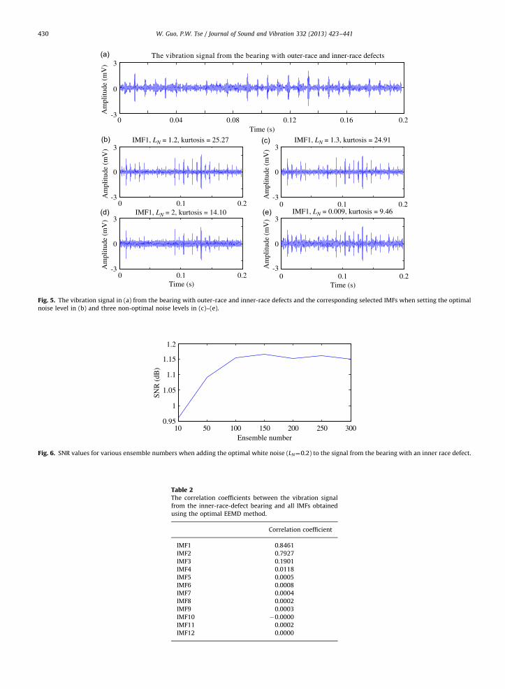
3.3.2.2. Decomposition of the signal from a bearing with multiple defects (the outer-race and inner-race defects). The secondexperimental signal, shown in Fig. 5(a), was collected from a faulty bearing in which there were defects on both the outerand the inner races. The relative RMSEs for different noise levels are shown in Fig. 4. The optimal noise level for this signal

-2
0
2
-2
0
2IMF1, LN = 0.2, kurtosis = 12.86
-2
0
2IMF1, LN = 1.4, kurtosis = 10.20
-2
0
2IMF1, LN = 2, kurtosis = 8.55
-2
0
2IMF1, LN = 0.009, kurtosis = 3.98
The vibration signal from the bearing with an inner race defect
0 0.04 0.08 0.12 0.16 0.2Time (s)
0 0.1 0.2 0 0.1 0.2
0 0.1 0.2 0 0.1 0.2Time (s)Time (s)
Am
plitu
de (
mV
)A
mpl
itude
(m
V)
Am
plitu
de (
mV
)A
mpl
itude
(m
V)
Am
plitu
de (
mV
)
Fig. 3. The vibration signal in (a) from the bearing with an inner race defect and the corresponding selected IMFs when setting the optimal noise level in
(b) and three non-optimal noise levels in (c)–(e).
0
0.2
0.4
0.6
0.8Relative RMSE
2 1 0.1 0.01 0.001Noise level
Noise level = 1.2
Fig. 4. Relative RMSEs when adding the white noise with various noise levels to the vibration signal from the bearing with outer-race and inner-race
defects. The optimal noise level for this signal is 1.2.
W. Guo, P.W. Tse / Journal of Sound and Vibration 332 (2013) 423–441 429
is 1.2. The selected IMF (IMF1) is shown in Fig. 5(b) and the kurtosis value is 25.27. Selecting the noise level, LN¼1.3,produces the second highest relative RMSE. The corresponding selected IMF and its kurtosis are shown in Fig. 5(c). Withthe noise level of LN¼2 or LN¼0.009, the selected IMFs shown in Fig. 5(d) and (e) contain more noise than previousdecomposition results. Their kurtosis values are also smaller: 14.10 and 9.46, respectively. Therefore, the optimal noiselevel for this vibration signal is 1.2.
Having determined the optimal noise level, the next step was to select an appropriate value for the ensemble number.In the experiments, the SNR was used to measure the remaining noise in the selected IMF and then determine theappropriate ensemble number. The higher the SNR value, the cleaner the signal. An example is used to illustrate thevariation in the SNR as the ensemble number increases. The example signal from the bearing with an inner race defect isshown in Fig. 3(a) and its optimal noise level is 0.2. The SNR values for the increased ensemble values are shown in Fig. 6.As shown in this figure, when the ensemble number is less than 100, increasing the ensemble number accelerates theincrease in the SNR value. When the ensemble number is larger than 150, the change in the SNR value is relatively small.Further increasing the ensemble number is ineffective for improving the SNR value. The real optimization process thusstopped at this point, NE¼150.
Therefore, for the bearing with an inner race defect, the corresponding vibration signal in Fig. 3(a), betterdecomposition performance can be obtained by setting the optimal noise level, LN¼0.2, and the ensemble number,NE¼150. Table 2 lists the correlation coefficients between the original vibration signal and all IMFs obtained using theoptimal EEMD method. The first three coefficients are much larger than the others, and the fourth coefficient is smaller.The coefficients of the other IMFs are close to zeros. To save space, only the first four IMFs are given here. The top diagram
-3
0
3
-3
0
3IMF1, LN = 1.2, kurtosis = 25.27
-3
0
3IMF1, LN = 1.3, kurtosis = 24.91
-3
0
3IMF1, LN = 2, kurtosis = 14.10
-3
0
3IMF1, LN = 0.009, kurtosis = 9.46
0 0.04 0.08 0.12 0.16 0.2Time (s)
0 0.1 0.2 0 0.1 0.2
0 0.1 0.2 0.1 0.2Time (s)Time (s)
0
The vibration signal from the bearing with outer-race and inner-race defects
Am
plitu
de (
mV
)A
mpl
itude
(m
V)
Am
plitu
de (
mV
)A
mpl
itude
(m
V)
Am
plitu
de (
mV
)
Fig. 5. The vibration signal in (a) from the bearing with outer-race and inner-race defects and the corresponding selected IMFs when setting the optimal
noise level in (b) and three non-optimal noise levels in (c)–(e).
10 50 100 150 200 250 3000.95
1
1.05
1.1
1.15
1.2
Ensemble number
SNR
(dB
)
Fig. 6. SNR values for various ensemble numbers when adding the optimal white noise (LN¼0.2) to the signal from the bearing with an inner race defect.
Table 2The correlation coefficients between the vibration signal
from the inner-race-defect bearing and all IMFs obtained
using the optimal EEMD method.
Correlation coefficient
IMF1 0.8461
IMF2 0.7927
IMF3 0.1901
IMF4 0.0118
IMF5 0.0005
IMF6 0.0008
IMF7 0.0004
IMF8 0.0002
IMF9 0.0003
IMF10 �0.0000
IMF11 0.0002
IMF12 0.0000
W. Guo, P.W. Tse / Journal of Sound and Vibration 332 (2013) 423–441430

-202
-202
-202
-101
-0.10
0.1
0 0.04 0.08 0.12 0.16 0.2
The vibration signal from the bearing with an inner race defect
IMF1
IMF2
IMF3
IMF4
Time (s)
Am
plitu
de (
mV
)
-3
0
3
-3
0
3
-3
0
3
-1
0
1
-1
0
1
0 0.04 0.08 0.12 0.16 0.2Time (s)
The vibration signal from the bearing with outer and inner race defects
IMF1
IMF2
IMF3
IMF4
Am
plitu
de (
mV
)
Fig. 7. Vibration signals collected from various faulty bearings and their corresponding first four IMFs decomposed using the optimal EEMD method.
(a) The vibration signal from the bearing with an inner race defect and the first four IMFs and (b) The vibration signal from the bearing with outer-race
and inner-race defects and the first four IMFs.
W. Guo, P.W. Tse / Journal of Sound and Vibration 332 (2013) 423–441 431
of Fig. 7(a) shows the original vibration signal and the remaining four diagrams show the first four IMFs extracted from theoriginal signal.
The decomposition results for the other vibration signal are shown in Fig. 7(b). The top diagram of Fig. 7(b) is the originalvibration signal. The remaining diagrams in this figure show main decomposition results, IMF1–IMF4. Comparing the originalvibration signal from each faulty bearing with the corresponding selected IMF (IMF1), it is clear that noise and the other irrelevantsignal components are removed and the extracted impulses in IMF1 are closely related to the characteristics of the faulty bearing.
3.3.3. Computation time analysis and stepped-up strategies
The EEMD method with parameter optimization is a repeated signal decomposition process. To analyze computationtime for the parameter optimization, the following assumptions are made:
1)
When setting the initial ensemble number and any value of noise level, the time of signal decomposition using theEEMD method is T1.2)
When optimizing the noise level, the number of levels between the initial noise level and the final level is N1; i.e., thesignal decomposition using EEMD is repeated N1 times to find the optimal noise level.3)
When searching an appropriate ensemble number for the signal to be analyzed, each ensemble number between theinitial value and the final value is a multiple of the initial ensemble number, ni (i¼1,2,y).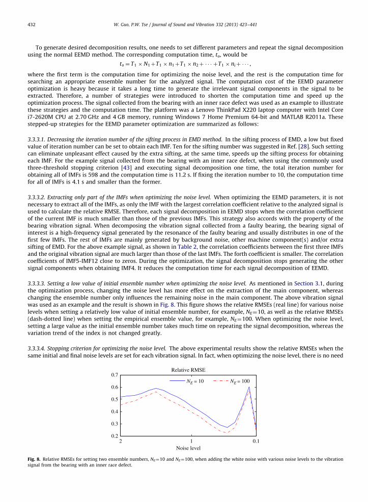
W. Guo, P.W. Tse / Journal of Sound and Vibration 332 (2013) 423–441432
To generate desired decomposition results, one needs to set different parameters and repeat the signal decompositionusing the normal EEMD method. The corresponding computation time, to, would be
to ¼ T1 � N1þT1 � n1þT1 � n2þ � � � þT1 � niþ � � � ,
where the first term is the computation time for optimizing the noise level, and the rest is the computation time forsearching an appropriate ensemble number for the analyzed signal. The computation cost of the EEMD parameteroptimization is heavy because it takes a long time to generate the irrelevant signal components in the signal to beextracted. Therefore, a number of strategies were introduced to shorten the computation time and speed up theoptimization process. The signal collected from the bearing with an inner race defect was used as an example to illustratethese strategies and the computation time. The platform was a Lenovo ThinkPad X220 laptop computer with Intel Corei7-2620M CPU at 2.70 GHz and 4 GB memory, running Windows 7 Home Premium 64-bit and MATLAB R2011a. Thesestepped-up strategies for the EEMD parameter optimization are summarized as follows:
3.3.3.1. Decreasing the iteration number of the sifting process in EMD method. In the sifting process of EMD, a low but fixedvalue of iteration number can be set to obtain each IMF. Ten for the sifting number was suggested in Ref. [28]. Such settingcan eliminate unpleasant effect caused by the extra sifting, at the same time, speeds up the sifting process for obtainingeach IMF. For the example signal collected from the bearing with an inner race defect, when using the commonly usedthree-threshold stopping criterion [43] and executing signal decomposition one time, the total iteration number forobtaining all of IMFs is 598 and the computation time is 11.2 s. If fixing the iteration number to 10, the computation timefor all of IMFs is 4.1 s and smaller than the former.
3.3.3.2. Extracting only part of the IMFs when optimizing the noise level. When optimizing the EEMD parameters, it is notnecessary to extract all of the IMFs, as only the IMF with the largest correlation coefficient relative to the analyzed signal isused to calculate the relative RMSE. Therefore, each signal decomposition in EEMD stops when the correlation coefficientof the current IMF is much smaller than those of the previous IMFs. This strategy also accords with the property of thebearing vibration signal. When decomposing the vibration signal collected from a faulty bearing, the bearing signal ofinterest is a high-frequency signal generated by the resonance of the faulty bearing and usually distributes in one of thefirst few IMFs. The rest of IMFs are mainly generated by background noise, other machine component(s) and/or extrasifting of EMD. For the above example signal, as shown in Table 2, the correlation coefficients between the first three IMFsand the original vibration signal are much larger than those of the last IMFs. The forth coefficient is smaller. The correlationcoefficients of IMF5-IMF12 close to zeros. During the optimization, the signal decomposition stops generating the othersignal components when obtaining IMF4. It reduces the computation time for each signal decomposition of EEMD.
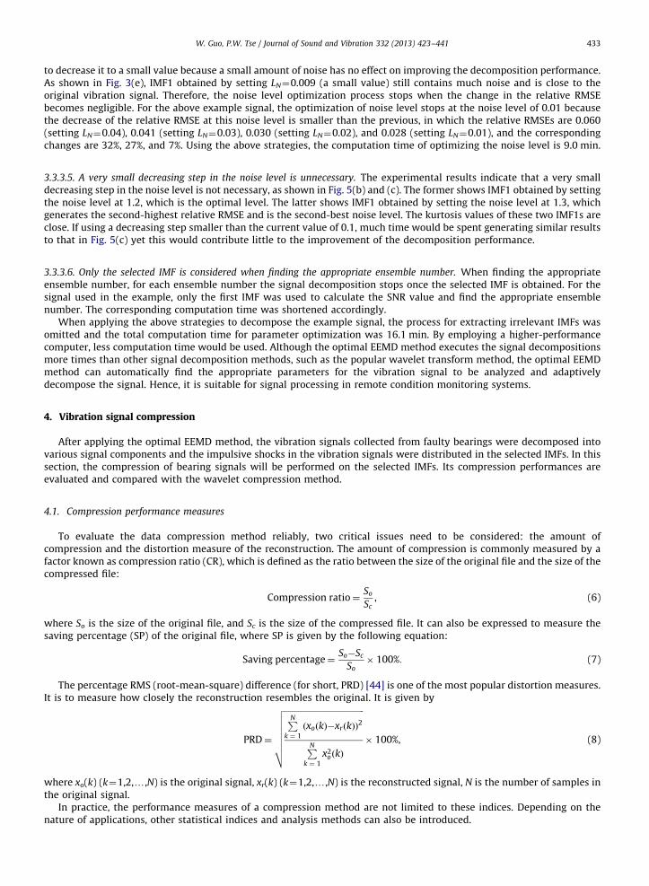
3.3.3.3. Setting a low value of initial ensemble number when optimizing the noise level. As mentioned in Section 3.1, duringthe optimization process, changing the noise level has more effect on the extraction of the main component, whereaschanging the ensemble number only influences the remaining noise in the main component. The above vibration signalwas used as an example and the result is shown in Fig. 8. This figure shows the relative RMSEs (real line) for various noiselevels when setting a relatively low value of initial ensemble number, for example, NE¼10, as well as the relative RMSEs(dash-dotted line) when setting the empirical ensemble value, for example, NE¼100. When optimizing the noise level,setting a large value as the initial ensemble number takes much time on repeating the signal decomposition, whereas thevariation trend of the index is not changed greatly.
3.3.3.4. Stopping criterion for optimizing the noise level. The above experimental results show the relative RMSEs when thesame initial and final noise levels are set for each vibration signal. In fact, when optimizing the noise level, there is no need
1 0.10.2
0.3
0.4
0.5
0.6
0.7
2
NE = 10 NE = 100
Relative RMSE
Noise level
Fig. 8. Relative RMSEs for setting two ensemble numbers, NE¼10 and NE¼100, when adding the white noise with various noise levels to the vibration
signal from the bearing with an inner race defect.
W. Guo, P.W. Tse / Journal of Sound and Vibration 332 (2013) 423–441 433
to decrease it to a small value because a small amount of noise has no effect on improving the decomposition performance.As shown in Fig. 3(e), IMF1 obtained by setting LN¼0.009 (a small value) still contains much noise and is close to theoriginal vibration signal. Therefore, the noise level optimization process stops when the change in the relative RMSEbecomes negligible. For the above example signal, the optimization of noise level stops at the noise level of 0.01 becausethe decrease of the relative RMSE at this noise level is smaller than the previous, in which the relative RMSEs are 0.060(setting LN¼0.04), 0.041 (setting LN¼0.03), 0.030 (setting LN¼0.02), and 0.028 (setting LN¼0.01), and the correspondingchanges are 32%, 27%, and 7%. Using the above strategies, the computation time of optimizing the noise level is 9.0 min.
3.3.3.5. A very small decreasing step in the noise level is unnecessary. The experimental results indicate that a very smalldecreasing step in the noise level is not necessary, as shown in Fig. 5(b) and (c). The former shows IMF1 obtained by settingthe noise level at 1.2, which is the optimal level. The latter shows IMF1 obtained by setting the noise level at 1.3, whichgenerates the second-highest relative RMSE and is the second-best noise level. The kurtosis values of these two IMF1s areclose. If using a decreasing step smaller than the current value of 0.1, much time would be spent generating similar resultsto that in Fig. 5(c) yet this would contribute little to the improvement of the decomposition performance.
3.3.3.6. Only the selected IMF is considered when finding the appropriate ensemble number. When finding the appropriateensemble number, for each ensemble number the signal decomposition stops once the selected IMF is obtained. For thesignal used in the example, only the first IMF was used to calculate the SNR value and find the appropriate ensemblenumber. The corresponding computation time was shortened accordingly.
When applying the above strategies to decompose the example signal, the process for extracting irrelevant IMFs wasomitted and the total computation time for parameter optimization was 16.1 min. By employing a higher-performancecomputer, less computation time would be used. Although the optimal EEMD method executes the signal decompositionsmore times than other signal decomposition methods, such as the popular wavelet transform method, the optimal EEMDmethod can automatically find the appropriate parameters for the vibration signal to be analyzed and adaptivelydecompose the signal. Hence, it is suitable for signal processing in remote condition monitoring systems.
4. Vibration signal compression
After applying the optimal EEMD method, the vibration signals collected from faulty bearings were decomposed intovarious signal components and the impulsive shocks in the vibration signals were distributed in the selected IMFs. In thissection, the compression of bearing signals will be performed on the selected IMFs. Its compression performances areevaluated and compared with the wavelet compression method.
4.1. Compression performance measures
To evaluate the data compression method reliably, two critical issues need to be considered: the amount ofcompression and the distortion measure of the reconstruction. The amount of compression is commonly measured by afactor known as compression ratio (CR), which is defined as the ratio between the size of the original file and the size of thecompressed file:
Compression ratio¼So
Sc, (6)
where So is the size of the original file, and Sc is the size of the compressed file. It can also be expressed to measure thesaving percentage (SP) of the original file, where SP is given by the following equation:
Saving percentage¼So�Sc
So� 100%: (7)
The percentage RMS (root-mean-square) difference (for short, PRD) [44] is one of the most popular distortion measures.It is to measure how closely the reconstruction resembles the original. It is given by
PRD¼
ffiffiffiffiffiffiffiffiffiffiffiffiffiffiffiffiffiffiffiffiffiffiffiffiffiffiffiffiffiffiffiffiffiffiffiffiffiffiffiPN
k ¼ 1
ðxoðkÞ�xrðkÞÞ2
PNk ¼ 1
x2oðkÞ
vuuuuuut � 100%, (8)
where xo(k) (k¼1,2,y,N) is the original signal, xr(k) (k¼1,2,y,N) is the reconstructed signal, N is the number of samples inthe original signal.
In practice, the performance measures of a compression method are not limited to these indices. Depending on thenature of applications, other statistical indices and analysis methods can also be introduced.
W. Guo, P.W. Tse / Journal of Sound and Vibration 332 (2013) 423–441434
4.2. Signal compressions and performance comparison
4.2.1. IMF-based signal compression
After applying the optimal EEMD method, the impulses generated by the faulty bearing are distributed in the selectedIMF and are separated from noise and other irrelevant signal components in the original signal. Such an IMF has a higherkurtosis value and thus can be compressed more efficiently than the original vibration signal can.
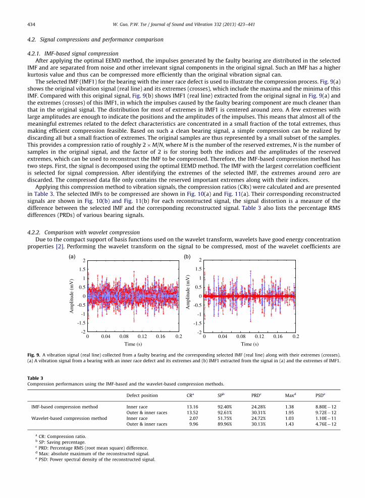
The selected IMF (IMF1) for the bearing with the inner race defect is used to illustrate the compression process. Fig. 9(a)shows the original vibration signal (real line) and its extremes (crosses), which include the maxima and the minima of thisIMF. Compared with this original signal, Fig. 9(b) shows IMF1 (real line) extracted from the original signal in Fig. 9(a) andthe extremes (crosses) of this IMF1, in which the impulses caused by the faulty bearing component are much cleaner thanthat in the original signal. The distribution for most of extremes in IMF1 is centered around zero. A few extremes withlarge amplitudes are enough to indicate the positions and the amplitudes of the impulses. This means that almost all of themeaningful extremes related to the defect characteristics are concentrated in a small fraction of the total extremes, thusmaking efficient compression feasible. Based on such a clean bearing signal, a simple compression can be realized bydiscarding all but a small fraction of extremes. The original samples are thus represented by a small subset of the samples.This provides a compression ratio of roughly 2�M/N, where M is the number of the reserved extremes, N is the number ofsamples in the original signal, and the factor of 2 is for storing both the indices and the amplitudes of the reservedextremes, which can be used to reconstruct the IMF to be compressed. Therefore, the IMF-based compression method hastwo steps. First, the signal is decomposed using the optimal EEMD method. The IMF with the largest correlation coefficientis selected for signal compression. After identifying the extremes of the selected IMF, the extremes around zero arediscarded. The compressed data file only contains the reserved important extremes along with their indices.
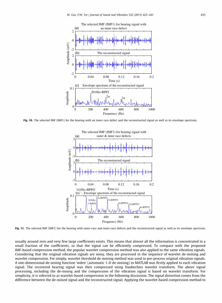
Applying this compression method to vibration signals, the compression ratios (CRs) were calculated and are presentedin Table 3. The selected IMFs to be compressed are shown in Fig. 10(a) and Fig. 11(a). Their corresponding reconstructedsignals are shown in Fig. 10(b) and Fig. 11(b) For each reconstructed signal, the signal distortion is a measure of thedifference between the selected IMF and the corresponding reconstructed signal. Table 3 also lists the percentage RMSdifferences (PRDs) of various bearing signals.
4.2.2. Comparison with wavelet compression
Due to the compact support of basis functions used on the wavelet transform, wavelets have good energy concentrationproperties [2]. Performing the wavelet transform on the signal to be compressed, most of the wavelet coefficients are
-2
-1.5
-1
-0.5
0
0.5
1
1.5
2
0 0.04 0.08 0.12 0.16 0.2
Time (s)
Am
plitu
de (
mV
)
-2
-1.5
-1
-0.5
0
0.5
1
1.5
2
0 0.04 0.08 0.12 0.16 0.2
Time (s)
Am
plitu
de (
mV
)
Fig. 9. A vibration signal (real line) collected from a faulty bearing and the corresponding selected IMF (real line) along with their extremes (crosses).
(a) A vibration signal from a bearing with an inner race defect and its extremes and (b) IMF1 extracted from the signal in (a) and the extremes of IMF1.
Table 3Compression performances using the IMF-based and the wavelet-based compression methods.
Defect position CRa SPb PRDc Maxd PSDe
IMF-based compression method Inner race 13.16 92.40% 24.28% 1.38 8.80E�12
Outer & inner races 13.52 92.61% 30.31% 1.95 9.72E�12
Wavelet-based compression method Inner race 2.07 51.75% 24.72% 1.03 1.10E�11
Outer & inner races 9.96 89.96% 30.13% 1.43 4.76E�12
a CR: Compression ratio.b SP: Saving percentage.c PRD: Percentage RMS (root mean square) difference.d Max: absolute maximum of the reconstructed signal.e PSD: Power spectral density of the reconstructed signal.
-2
0
2
-2
0
2The reconstructed signal
0 200 400 600 8000
0.1Envelope spectrum of the reconstructed signal
0 0.04 0.08 0.12 0.16 0.2Time (s)
Frequency (Hz)
201Hz≈BPFI2× 3×
Am
plitu
de (
mV
)A
mpl
itude
The selected IMF (IMF1) for bearing signal withan inner race defect
1000
Fig. 10. The selected IMF (IMF1) for the bearing with an inner race defect and the reconstructed signal as well as its envelope spectrum.
-3
0
3
0 0.04 0.08 0.12 0.16 0.2-3
0
3The reconstructed signal
0 200 400 600 800 10000
0.1Envelope spectrum of the reconstructed signal
Time (s)
Frequency (Hz)
141Hz≈BPFO
3×BPFO2×BPFO
205Hz≈ BPFI 4×BPFO 5×BPFO
6×BPFO
Am
plitu
de (
mV
)A
mpl
itude
The selected IMF (IMF1) for bearing signal withouter & inner race defects
Fig. 11. The selected IMF (IMF1) for the bearing with outer-race and inner-race defects and the reconstructed signal as well as its envelope spectrum.
W. Guo, P.W. Tse / Journal of Sound and Vibration 332 (2013) 423–441 435
usually around zero and very few large coefficients exists. This means that almost all the information is concentrated in asmall fraction of the coefficients, so that the signal can be efficiently compressed. To compare with the proposedIMF-based compression method, the popular wavelet compression method was also applied to the same vibration signals.Considering that the original vibration signals are noisy, they are processed in the sequence of wavelet de-noising andwavelet compression. For simply, wavelet threshold de-noising method was used to pre-process original vibration signals.A one-dimensional de-nosing function ‘wden’ (automatic 1-D de-noising) in MATLAB was firstly applied to each vibrationsignal. The recovered bearing signal was then compressed using Daubechies wavelet transform. The above signalprocessing, including the de-nosing and the compression of the vibration signal is based on wavelet transform. Forsimplicity, it is referred to as wavelet-based compression in the following discussion. The signal distortion comes from thedifference between the de-noised signal and the reconstructed signal. Applying the wavelet-based compression method to

-2
0
2The vibration signal from the bearing with an inner race defect
-2
0
2The reconstructed signal for the IMF-based compression
-2
0
2The reconstructed signal for wavelet-based compression
0 0.04 0.08 0.12 0.16 0.2Time (s)
Am
plitu
de (
mV
)
-3
0
3The vibration signal from bearing with outer and inner race defects
-3
0
3The reconstructed signal for the IMF-based compression
-3
0
3The reconstructed signal for wavelet-based compression
0 0.04 0.08 0.12 0.16 0.2Time (s)
Am
plitu
de (
mV
)
Fig. 12. Vibration signals from various faulty bearings and their corresponding reconstructed signals for the IMF-based and the wavelet-based
compression methods. (a) Original and reconstructed signals for the bearing with an inner race defect and (b) Original and reconstructed signals for the
bearing with outer-race and inner-race defects.
W. Guo, P.W. Tse / Journal of Sound and Vibration 332 (2013) 423–441436
the above vibration signals, the same performance measures, CR and PRD, were calculated and are also presented inTable 3. Their reconstructed signals are shown in the bottom diagrams of Fig. 12(a) and (b).
For the bearing with an inner race defect, the original vibration signal is also shown in the top diagram of Fig. 12(a).After compressing this vibration signal, the reconstructed signals for the proposed IMF-based compression and thewavelet-based compression are shown in the middle and the bottom diagrams of Fig. 12(a), respectively. The CR, SP, andPRD using the IMF-based compression method are 13.16, 92.40%, and 24.28%, respectively. However, using the wavelet-based compression method, the PRD is 24.72% which is close to 24.28%, and the CR is only 2.07 (SP¼51.75%). The IMF-based compression method has a much higher compression ratio with a similar signal distortion.
For another faulty bearing, the original vibration signal is shown in the top diagram of Fig. 12(b), and the reconstructedsignals for these two compressions are displayed in the middle and the bottom diagrams of Fig. 12(b). The compressionmeasures are shown in the rows denoted as ‘Outer & inner races’ in Table 3. Using the wavelet-based compression method,the CR is 9.96 (SP¼89.96%) and the PRD is 30.13%. In comparison, the proposed IMF-based compression provides a slightlybetter compression result, in which the CR is 13.52 (SP¼92.61%) and the PRD is 30.31%.
The comparisons of experimental results indicates that the performance of the IMF-based compression is better thanthe wavelet-based compression for the same vibration signal. In addition to the above two performance measures, theabsolute maximum value and the power spectral density (PSD) were also calculated to compare the reconstructed signalsfor two compression methods, which are listed in the last two columns of Table 3. For example, for the bearing with themultiple defects, applying the wavelet-based compression method to this vibration signal, the absolute maximum valueand the PSD of the reconstructed signal are 1.43 and 4.76E�12, respectively. Applying the IMF-based compression methodto the same vibration signal, the absolute maximum value and the PSD of the reconstructed signal are higher, 1.95 and9.72E�12, respectively. The difference on the maximum values can be directly observed from the reconstructed signals
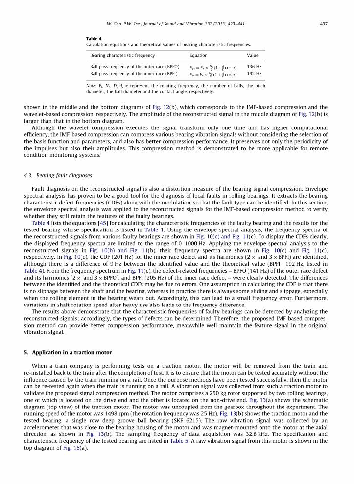
Table 4Calculation equations and theoretical values of bearing characteristic frequencies.
Bearing characteristic frequency Equation Value
Ball pass frequency of the outer race (BPFO) For ¼ Fr �Nb2 ð1�
dD cos aÞ 136 Hz
Ball pass frequency of the inner race (BPFI) Fir ¼ Fr �Nb2 ð1þ
dD cos aÞ 192 Hz
Note: Fr, Nb, D, d, a represent the rotating frequency, the number of balls, the pitch
diameter, the ball diameter and the contact angle, respectively.
W. Guo, P.W. Tse / Journal of Sound and Vibration 332 (2013) 423–441 437
shown in the middle and the bottom diagrams of Fig. 12(b), which corresponds to the IMF-based compression and thewavelet-based compression, respectively. The amplitude of the reconstructed signal in the middle diagram of Fig. 12(b) islarger than that in the bottom diagram.
Although the wavelet compression executes the signal transform only one time and has higher computationalefficiency, the IMF-based compression can compress various bearing vibration signals without considering the selection ofthe basis function and parameters, and also has better compression performance. It preserves not only the periodicity ofthe impulses but also their amplitudes. This compression method is demonstrated to be more applicable for remotecondition monitoring systems.
4.3. Bearing fault diagnoses
Fault diagnosis on the reconstructed signal is also a distortion measure of the bearing signal compression. Envelopespectral analysis has proven to be a good tool for the diagnosis of local faults in rolling bearings. It extracts the bearingcharacteristic defect frequencies (CDFs) along with the modulation, so that the fault type can be identified. In this section,the envelope spectral analysis was applied to the reconstructed signals for the IMF-based compression method to verifywhether they still retain the features of the faulty bearings.
Table 4 lists the equations [45] for calculating the characteristic frequencies of the faulty bearing and the results for thetested bearing whose specification is listed in Table 1. Using the envelope spectral analysis, the frequency spectra ofthe reconstructed signals from various faulty bearings are shown in Fig. 10(c) and Fig. 11(c). To display the CDFs clearly,the displayed frequency spectra are limited to the range of 0–1000 Hz. Applying the envelope spectral analysis to thereconstructed signals in Fig. 10(b) and Fig. 11(b), their frequency spectra are shown in Fig. 10(c) and Fig. 11(c),respectively. In Fig. 10(c), the CDF (201 Hz) for the inner race defect and its harmonics (2� and 3�BPFI) are identified,although there is a difference of 9 Hz between the identified value and the theoretical value (BPFI¼192 Hz, listed inTable 4). From the frequency spectrum in Fig. 11(c), the defect-related frequencies – BPFO (141 Hz) of the outer race defectand its harmonics (2� and 3�BPFO), and BPFI (205 Hz) of the inner race defect – were clearly detected. The differencesbetween the identified and the theoretical CDFs may be due to errors. One assumption in calculating the CDF is that thereis no slippage between the shaft and the bearing, whereas in practice there is always some sliding and slippage, especiallywhen the rolling element in the bearing wears out. Accordingly, this can lead to a small frequency error. Furthermore,variations in shaft rotation speed after heavy use also leads to the frequency difference.
The results above demonstrate that the characteristic frequencies of faulty bearings can be detected by analyzing thereconstructed signals; accordingly, the types of defects can be determined. Therefore, the proposed IMF-based compres-sion method can provide better compression performance, meanwhile well maintain the feature signal in the originalvibration signal.
5. Application in a traction motor
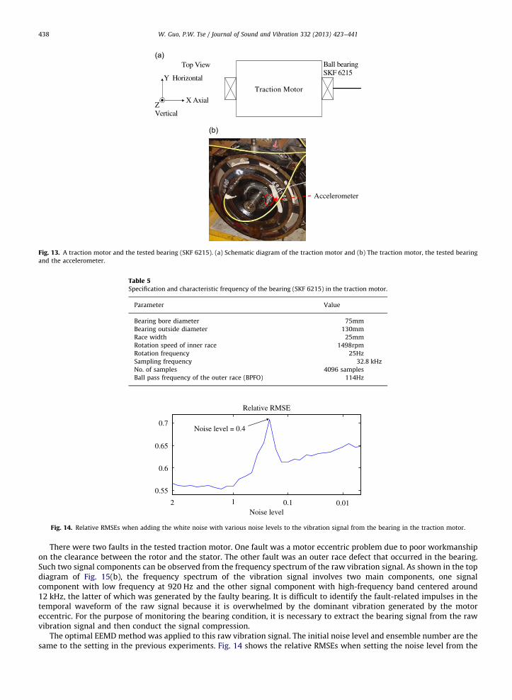
When a train company is performing tests on a traction motor, the motor will be removed from the train andre-installed back to the train after the completion of test. It is to ensure that the motor can be tested accurately without theinfluence caused by the train running on a rail. Once the purpose methods have been tested successfully, then the motorcan be re-tested again when the train is running on a rail. A vibration signal was collected from such a traction motor tovalidate the proposed signal compression method. The motor comprises a 250 kg rotor supported by two rolling bearings,one of which is located on the drive end and the other is located on the non-drive end. Fig. 13(a) shows the schematicdiagram (top view) of the traction motor. The motor was uncoupled from the gearbox throughout the experiment. Therunning speed of the motor was 1498 rpm (the rotation frequency was 25 Hz). Fig. 13(b) shows the traction motor and thetested bearing, a single row deep groove ball bearing (SKF 6215). The raw vibration signal was collected by anaccelerometer that was close to the bearing housing of the motor and was magnet-mounted onto the motor at the axialdirection, as shown in Fig. 13(b). The sampling frequency of data acquisition was 32.8 kHz. The specification andcharacteristic frequency of the tested bearing are listed in Table 5. A raw vibration signal from this motor is shown in thetop diagram of Fig. 15(a).
Ball bearingSKF 6215
Traction Motor
Y Horizontal
X AxialZVertical
Top View
Accelerometer
Fig. 13. A traction motor and the tested bearing (SKF 6215). (a) Schematic diagram of the traction motor and (b) The traction motor, the tested bearing
and the accelerometer.
Table 5Specification and characteristic frequency of the bearing (SKF 6215) in the traction motor.
Parameter Value
Bearing bore diameter 75mm
Bearing outside diameter 130mm
Race width 25mm
Rotation speed of inner race 1498rpm
Rotation frequency 25Hz
Sampling frequency 32.8 kHz
No. of samples 4096 samples
Ball pass frequency of the outer race (BPFO) 114Hz
2 1 0.1 0.01Noise level
Relative RMSE
Noise level = 0.4
0.55
0.6
0.65
0.7
Fig. 14. Relative RMSEs when adding the white noise with various noise levels to the vibration signal from the bearing in the traction motor.
W. Guo, P.W. Tse / Journal of Sound and Vibration 332 (2013) 423–441438
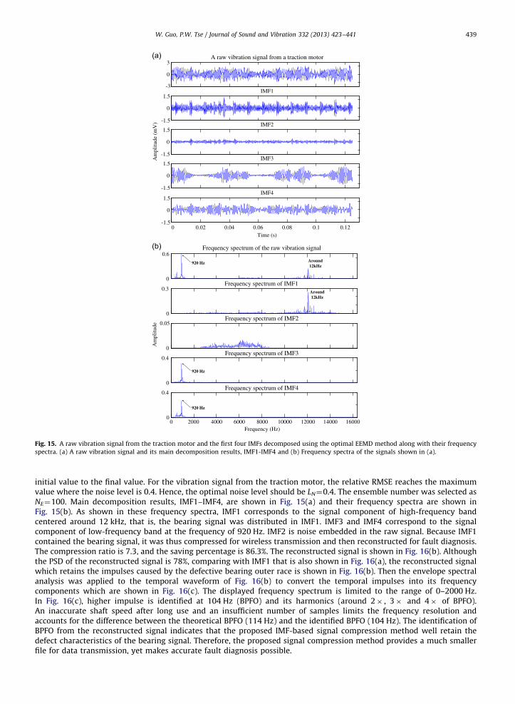
There were two faults in the tested traction motor. One fault was a motor eccentric problem due to poor workmanshipon the clearance between the rotor and the stator. The other fault was an outer race defect that occurred in the bearing.Such two signal components can be observed from the frequency spectrum of the raw vibration signal. As shown in the topdiagram of Fig. 15(b), the frequency spectrum of the vibration signal involves two main components, one signalcomponent with low frequency at 920 Hz and the other signal component with high-frequency band centered around12 kHz, the latter of which was generated by the faulty bearing. It is difficult to identify the fault-related impulses in thetemporal waveform of the raw signal because it is overwhelmed by the dominant vibration generated by the motoreccentric. For the purpose of monitoring the bearing condition, it is necessary to extract the bearing signal from the rawvibration signal and then conduct the signal compression.
The optimal EEMD method was applied to this raw vibration signal. The initial noise level and ensemble number are thesame to the setting in the previous experiments. Fig. 14 shows the relative RMSEs when setting the noise level from the
-3
0
3A raw vibration signal from a traction motor
-1.5
0
1.5IMF1
IMF2
IMF3
0 0.02 0.04 0.06 0.08 0.1 0.12
IMF4
-1.5
0
1.5
-1.5
0
1.5
-1.5
0
1.5
Time (s)
Am
plitu
de(m
V)
0
0.6
0
0.3
0
0.05
0
0.4
0 2000 4000 6000 8000 10000 12000 14000 160000
0.4
Frequency spectrum of the raw vibration signal
Frequency spectrum of IMF1
Frequency spectrum of IMF2
Frequency spectrum of IMF3
Frequency spectrum of IMF4
Frequency (Hz)
Am
plit
ude
920 Hz Around12kHz
920 Hz
920 Hz
Around12kHz
Fig. 15. A raw vibration signal from the traction motor and the first four IMFs decomposed using the optimal EEMD method along with their frequency
spectra. (a) A raw vibration signal and its main decomposition results, IMF1-IMF4 and (b) Frequency spectra of the signals shown in (a).
W. Guo, P.W. Tse / Journal of Sound and Vibration 332 (2013) 423–441 439
initial value to the final value. For the vibration signal from the traction motor, the relative RMSE reaches the maximumvalue where the noise level is 0.4. Hence, the optimal noise level should be LN¼0.4. The ensemble number was selected asNE¼100. Main decomposition results, IMF1–IMF4, are shown in Fig. 15(a) and their frequency spectra are shown inFig. 15(b). As shown in these frequency spectra, IMF1 corresponds to the signal component of high-frequency bandcentered around 12 kHz, that is, the bearing signal was distributed in IMF1. IMF3 and IMF4 correspond to the signalcomponent of low-frequency band at the frequency of 920 Hz. IMF2 is noise embedded in the raw signal. Because IMF1contained the bearing signal, it was thus compressed for wireless transmission and then reconstructed for fault diagnosis.The compression ratio is 7.3, and the saving percentage is 86.3%. The reconstructed signal is shown in Fig. 16(b). Althoughthe PSD of the reconstructed signal is 78%, comparing with IMF1 that is also shown in Fig. 16(a), the reconstructed signalwhich retains the impulses caused by the defective bearing outer race is shown in Fig. 16(b). Then the envelope spectralanalysis was applied to the temporal waveform of Fig. 16(b) to convert the temporal impulses into its frequencycomponents which are shown in Fig. 16(c). The displayed frequency spectrum is limited to the range of 0–2000 Hz.In Fig. 16(c), higher impulse is identified at 104 Hz (BPFO) and its harmonics (around 2� , 3� and 4� of BPFO).An inaccurate shaft speed after long use and an insufficient number of samples limits the frequency resolution andaccounts for the difference between the theoretical BPFO (114 Hz) and the identified BPFO (104 Hz). The identification ofBPFO from the reconstructed signal indicates that the proposed IMF-based signal compression method well retain thedefect characteristics of the bearing signal. Therefore, the proposed signal compression method provides a much smallerfile for data transmission, yet makes accurate fault diagnosis possible.
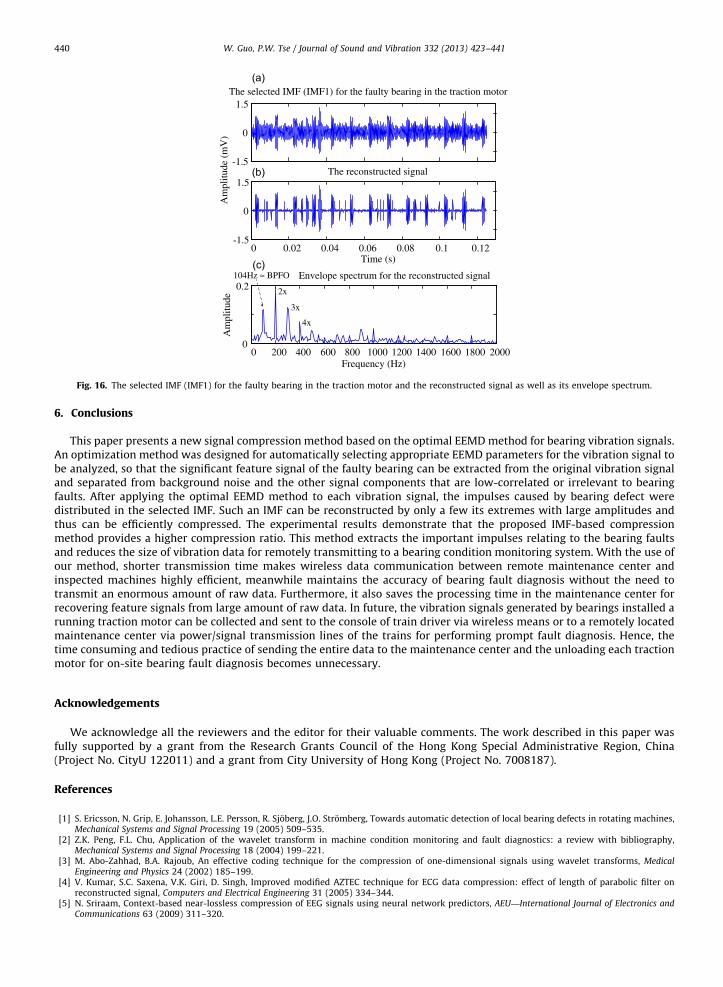
-1.5
0
1.5The selected IMF (IMF1) for the faulty bearing in the traction motor
0 0.02 0.04 0.06 0.08 0.1 0.12
The reconstructed signal
0 200 400 600 800 1000 1200 1400 1600 1800 20000
0.2Envelope spectrum for the reconstructed signal
-1.5
0
1.5
104Hz ≈ BPFO
2x
3x
4x
Time (s)
Frequency (Hz)
Am
plitu
de(m
V)
Am
plitu
de
Fig. 16. The selected IMF (IMF1) for the faulty bearing in the traction motor and the reconstructed signal as well as its envelope spectrum.
W. Guo, P.W. Tse / Journal of Sound and Vibration 332 (2013) 423–441440
6. Conclusions
This paper presents a new signal compression method based on the optimal EEMD method for bearing vibration signals.An optimization method was designed for automatically selecting appropriate EEMD parameters for the vibration signal tobe analyzed, so that the significant feature signal of the faulty bearing can be extracted from the original vibration signaland separated from background noise and the other signal components that are low-correlated or irrelevant to bearingfaults. After applying the optimal EEMD method to each vibration signal, the impulses caused by bearing defect weredistributed in the selected IMF. Such an IMF can be reconstructed by only a few its extremes with large amplitudes andthus can be efficiently compressed. The experimental results demonstrate that the proposed IMF-based compressionmethod provides a higher compression ratio. This method extracts the important impulses relating to the bearing faultsand reduces the size of vibration data for remotely transmitting to a bearing condition monitoring system. With the use ofour method, shorter transmission time makes wireless data communication between remote maintenance center andinspected machines highly efficient, meanwhile maintains the accuracy of bearing fault diagnosis without the need totransmit an enormous amount of raw data. Furthermore, it also saves the processing time in the maintenance center forrecovering feature signals from large amount of raw data. In future, the vibration signals generated by bearings installed arunning traction motor can be collected and sent to the console of train driver via wireless means or to a remotely locatedmaintenance center via power/signal transmission lines of the trains for performing prompt fault diagnosis. Hence, thetime consuming and tedious practice of sending the entire data to the maintenance center and the unloading each tractionmotor for on-site bearing fault diagnosis becomes unnecessary.
Acknowledgements
We acknowledge all the reviewers and the editor for their valuable comments. The work described in this paper wasfully supported by a grant from the Research Grants Council of the Hong Kong Special Administrative Region, China(Project No. CityU 122011) and a grant from City University of Hong Kong (Project No. 7008187).
References
[1] S. Ericsson, N. Grip, E. Johansson, L.E. Persson, R. Sjoberg, J.O. Stromberg, Towards automatic detection of local bearing defects in rotating machines,Mechanical Systems and Signal Processing 19 (2005) 509–535.
[2] Z.K. Peng, F.L. Chu, Application of the wavelet transform in machine condition monitoring and fault diagnostics: a review with bibliography,Mechanical Systems and Signal Processing 18 (2004) 199–221.
[3] M. Abo-Zahhad, B.A. Rajoub, An effective coding technique for the compression of one-dimensional signals using wavelet transforms, MedicalEngineering and Physics 24 (2002) 185–199.
[4] V. Kumar, S.C. Saxena, V.K. Giri, D. Singh, Improved modified AZTEC technique for ECG data compression: effect of length of parabolic filter onreconstructed signal, Computers and Electrical Engineering 31 (2005) 334–344.
[5] N. Sriraam, Context-based near-lossless compression of EEG signals using neural network predictors, AEU—International Journal of Electronics andCommunications 63 (2009) 311–320.
W. Guo, P.W. Tse / Journal of Sound and Vibration 332 (2013) 423–441 441
[6] N. Sriraam, C. Eswaran, Performance evaluation of neural network and linear predictors for near-lossless compression of EEG signals, IEEETransactions on Information Technology in Biomedicine 12 (2008) 87–93.
[7] B. Li, P. Zhang, D. Liu, S. Mi, G. Ren, H. Tian, Feature extraction for rolling element bearing fault diagnosis utilizing generalized S transform and two-dimensional non-negative matrix factorization, Journal of Sound and Vibration 330 (2011) 2388–2399.
[8] C. Vijaya, J.S. Bhat, Signal compression using discrete fractional Fourier transform and set partitioning in hierarchical tree, Signal Processing 86 (2006)1976–1983.
[9] L.V. Batista, E.U.K. Melcher, L.C. Carvalho, Compression of ECG signals by optimized quantization of discrete cosine transform coefficients, MedicalEngineering and Physics 23 (2001) 127–134.
[10] W.J. Staszewski, Wavelet based compression and feature selection for vibration analysis, Journal of Sound and Vibration 211 (1998) 735–760.[11] I. Daubechies, Ten lectures on wavelets, Philadelphia, Society for Industrial and Applied Mathematics, Pa., 1992.[12] C.T. Ku, K.C. Hung, T.C. Wu, H.S. Wang, Wavelet-based ECG data compression system with linear quality control scheme, IEEE Transactions on
Biomedical Engineering 57 (2010) 1399–1409.[13] M. Blanco-Velasco, F. Cruz-Roldan, J.I. Godino-Llorente, K.E. Barner, Wavelet packets feasibility study for the design of an ECG compressor, IEEE
Transactions on Biomedical Engineering 54 (2007) 766–769.[14] B. Kotnik, Z. Kacic, A noise robust feature extraction algorithm using joint wavelet packet subband decomposition and AR modeling of speech
signals, Signal Processing 87 (2007) 1202–1223.[15] W.J. Staszewski, Vibration data compression with optimal wavelet coefficients, in: Genetic Algorithms in Engineering Systems: Innovations and
Applications, 1997. GALESIA 97. Second International Conference on (Conf. Publ. No. 446), 1997, pp. 186–190.[16] M. Tanaka, M. Sakawa, K. Kato, M. Abe, Application of wavelet transform to compression of mechanical vibration data, Cybernetics and Systems: An
International Journal 28 (1997) 225–244.[17] M. Xu, J. Zhang, G. Zhang, W. Huang, Method of data compressing for rotating machinery vibration signal based on wavelet transform, Journal of
Vibration Engineering 13 (2000) 531–536.[18] B. Liu, Selection of wavelet packet basis for rotating machinery fault diagnosis, Journal of Sound and Vibration 284 (2005) 567–582.[19] H. Qiu, J. Lee, J. Lin, G. Yu, Wavelet filter-based weak signature detection method and its application on rolling element bearing prognostics, Journal
of Sound and Vibration 289 (2006) 1066–1090.[20] Z.K. Peng, M.R. Jackson, J.A. Rongong, F.L. Chu, R.M. Parkin, On the energy leakage of discrete wavelet transform, Mechanical Systems and Signal
Processing 23 (2009) 330–343.[21] Z.K. Peng, P.W. Tse, F.L. Chu, An improved Hilbert–Huang transform and its application in vibration signal analysis, Journal of Sound and Vibration 286
(2005) 187–205.[22] N.E. Huang, Z. Shen, R. Long, C. Wu, H. Shih, Q. Zheng, C. Yen, C. Tung, H. Liu, The empirical mode decomposition and the Hilbert spectrum for
nonlinear and non-stationary time series analysis, in: Proceedings of the Royal Society of London Series A—Mathematical Physical and EngineerSciences 1998, pp. 903–995.
[23] N.E. Huang, Z. Shen, S.R. Long, A new view of nonlinear water waves—the Hilbert spectrum, Annual Review of Fluid Mechanics 31 (1999) 417–457.[24] M. Feldman, Analytical basics of the EMD: two harmonics decomposition, Mechanical Systems and Signal Processing 23 (2009) 2059–2071.[25] N.E. Huang, S.S.P. Shen, Hilbert–Huang Transform and Its Applications, World Scientific, Singapore; Hackensack, NJ; London, 2005.[26] D. Pines, L. Salvino, Structural health monitoring using empirical mode decomposition and the Hilbert phase, Journal of Sound and Vibration 294
(2006) 97–124.[27] Q. Miao, D. Wang, M. Pecht, A probabilistic description scheme for rotating machinery health evaluation, Journal of Mechanical Science and
Technology 24 (2010) 2421–2430.[28] Z. Wu, N.E. Huang, Ensemble empirical mode decomposition: a noise-assisted data analysis method, Advances in Adaptive Data Analysis 1 (2009)
1–41.[29] Y. Lei, Z. He, Y. Zi, Application of the EEMD method to rotor fault diagnosis of rotating machinery, Mechanical Systems and Signal Processing 23 (2009)
1327–1338.[30] Y. Lei, Z. He, Y. Zi, EEMD method and WNN for fault diagnosis of locomotive roller bearings, Expert Systems with Applications 38 (2011) 7334–7341.[31] Y. Lei, M.J. Zuo, Fault diagnosis of rotating machinery using an improved HHT based on EEMD and sensitive IMFs, Measurement Science and
Technology 20 (2009) 125701. 125712pp.[32] Y. Zhou, T. Tao, X. Mei, G. Jiang, N. Sun, Feed-axis gearbox condition monitoring using built-in position sensors and EEMD method, Robotics and
Computer-Integrated Manufacturing 27 (2011) 785–793.[33] T.Y. Wu, Y.L. Chung, Misalignment diagnosis of rotating machinery through vibration analysis via the hybrid EEMD and EMD approach, Smart
Materials and Structures 18 (2009) 095004.[34] L. Chen, X. Li, X.B. Li, Z.Y. Huang, Signal extraction using ensemble empirical mode decomposition and sparsity in pipeline magnetic flux leakage
nondestructive evaluation, Review of Scientific Instruments 80 (2009) 025105.[35] Z.H. Wu, N.E. Huang, X.Y. Chen, The multidimensional ensemble empirical mode decomposition method, Advances in Adaptive Data Analysis 1 (2009)
339–372.[36] M. Zvokelj, S. Zupan, I. Prebil, Multivariate and multiscale monitoring of large-size low-speed bearings using ensemble empirical mode
decomposition method combined with principal component analysis, Mechanical Systems and Signal Processing 24 (2010) 1049–1067.[37] M. Zvokelj, S. Zupan, I. Prebil, Nonlinear multivariate and multiscale monitoring and signal denoising strategy using Kernel principal component
analysis combined with ensemble empirical mode decomposition method, Mechanical Systems and Signal Processing 25 (2011) 2631–2653.[38] K.M. Chang, S.H. Liu, Gaussian noise filtering from ECG by Wiener filter and ensemble empirical mode decomposition, Journal of Signal Processing 64
(2011) 249–264.[39] J. Zhang, R. Yan, R.X. Gao, Z. Feng, Performance enhancement of ensemble empirical mode decomposition, Mechanical Systems and Signal Processing
24 (2010) 2104–2123.[40] J.R. Yeh, J.S. Shieh, N.E. Huang, Complementary ensemble empirical mode decomposition: a novel noise enhanced data analysis method, Advances in
Adaptive Data Analysis 2 (2010) 135–156.[41] R.K. Niazy, C.F. Beckmann, J.M. Brady, S.M. Smith, Performance evaluation of ensemble empirical mode decomposition, Advances in Adaptive Data
Analysis 1 (2009) 231–242.[42] W. Guo, P.W. Tse, Enhancing the ability of ensemble empirical mode decomposition in machine fault diagnosis, in: Proceedings of 2010 Prognostics
and System Health Management Conference, Macau, Jan. 2010, pp. 1–7.[43] G. Rilling, P. Flandrin, P. Goncalves, On empirical mode decomposition and its algorithms, in: Proceedings of the IEEE EURASIP Workshop on
Nonlinear Signal and Image Processing, Grado (I), June 2003, pp. 1–5.[44] G. Nave, A. Cohen, ECG compression using long-term prediction, IEEE Transactions on Biomedical Engineering 40 (1993) 877–885.[45] R.K. Mobley, An Introduction to Predictive Maintenance, second ed. Butterworth-Heinemann, Amsterdam; New York, 2002.
Related Documents


