A novel heuristic approach for distance- and connectivity-based multihop node localization in wireless sensor networks

ORIGINAL PAPER

A novel heuristic approach for distance- and connectivity-basedmultihop node localization in wireless sensor networks

Diana Manjarres • Javier Del Ser • Sergio Gil-Lopez •

Massimo Vecchio • Itziar Landa-Torres •

Roberto Lopez-Valcarce

Published online: 2 August 2012

� Springer-Verlag 2012

Abstract The availability of accurate location informa-

tion of constituent nodes becomes essential in many

applications of wireless sensor networks. In this context,

we focus on anchor-based networks where the position of

some few nodes are assumed to be fixed and known a

priori, whereas the location of all other nodes is to be

estimated based on noisy pairwise distance measurements.

This localization task embodies a non-convex optimization

problem which gets even more involved by the fact that

the network may not be uniquely localizable, especially

when its connectivity is not sufficiently high. To efficiently

tackle this problem, we present a novel soft computing

approach based on a hybridization of the Harmony Search

(HS) algorithm with a local search procedure that itera-

tively alleviates the aforementioned non-uniqueness of

sparse network deployments. Furthermore, the areas in

which sensor nodes can be located are limited by means

of connectivity-based geometrical constraints. Extensive

simulation results show that the proposed approach out-

performs previously published soft computing localization

techniques in most of the simulated topologies. In partic-

ular, to assess the effectiveness of the technique, we

compare its performance, in terms of Normalized Locali-

zation Error (NLE), to that of Simulated Annealing (SA)-

based and Particle Swarm Optimization (PSO)-based

techniques, as well as a naive implementation of a Genetic

Algorithm (GA) incorporating the same local search pro-

cedure here proposed. Non-parametric hypothesis tests are

also used so as to shed light on the statistical significance of

the obtained results.

Keywords Wireless sensor networks �Node localization � Flip ambiguity � Harmony search

1 Introduction

The last decade has witnessed an evergrowing research

interest in Wireless Sensor Networks (WSNs), which

consist of hundreds or even thousand of nodes operating

with high level of autonomy, while communicating to

each other without the need of any wired link (Akyildiz

et al. 2002). These densely-deployed sensor meshes per-

mit to efficiently monitor a wide range of physical

parameters in a cost-effective fashion. Originally restric-

ted to military and defense applications, recent advances

in wireless communications and electronics, along with

the availability of low-cost smart sensors, have made

WSNs also appealing for several emerging applications,

such as infrastructure security, habitat monitoring (e.g.

temperature, humidity, water, indoor air quality), preci-

sion agriculture, industrial sensing, traffic control, vehicle

and animal tracking, etc.

D. Manjarres � J. Del Ser (&) � S. Gil-Lopez � I. Landa-Torres

OPTIMA Unit, Tecnalia Research and Innovation, P.

Tecnologico, Ed. 202, 48170 Zamudio, Spain

e-mail: [email protected]

D. Manjarres

e-mail: [email protected]

S. Gil-Lopez

e-mail: [email protected]

I. Landa-Torres

e-mail: [email protected]

M. Vecchio � R. Lopez-Valcarce

Departamento de Teorıa de la Senal y las Comunicaciones,

University of Vigo, C/ Maxwell s/n, 36310 Vigo, Spain

e-mail: [email protected]

R. Lopez-Valcarce

e-mail: [email protected]

123

Soft Comput (2013) 17:17–28

DOI 10.1007/s00500-012-0897-2

In such applications, automatic and accurate location of

the underlying sensor nodes is highly desirable in order to

make collected data meaningful (Hu and Evans 2004).

Indeed, the knowledge of the location of the nodes plays an

important role in the design of efficient network routing

protocols and in security applications (Mauve et al. 2001).

However, due to the constraints on the size, the cost and the

limited energy available at sensor nodes, the installation of

a Global Positioning System (GPS) on each device is not

always feasible in practice, since it may jeopardize the

network autonomy. Furthermore, GPS is not accessible in

some environments, being generally not suitable for indoor

and underground deployments. Consequently, most of the

efforts so far have been aimed at developing alternative

approaches to this problem, and thereby localization in

WSNs is still deemed as an open research problem by the

scientific community.

In this context, we focus on the anchor-based WSN

scenario, where a few static nodes of the network (referred

to as anchor nodes) know their exact positions in advance

by means of either on-board GPS devices or their manual

placement beforehand. The main goal is to estimate the

coordinates of all non-anchor nodes, assuming that each

sensor can infer the distance (subject to some error) to its

neighbor nodes, based on Angle of Arrival (AoA) mea-

surements (Niculescu and Nath 2003), time-related mea-

surements such as Time of Arrival or Time Difference of

Arrival (Savvides et al. 2001) or Received Signal Strength

Indication (RSSI) profiling techniques (Alippi and Vanini

2006). In particular, we focus on the latter, for which the

most straightforward localization algorithm reduces to the

statistical Maximum Likelihood (ML) estimation method.

However, formalizing the localization problem as an ML

estimation results in a multivariate non-convex optimiza-

tion problem (More and Wu 1997), for which different

computationally-efficient approaches have been proposed

in the literature.

Localization techniques can be broadly classified into

one-hop and multi-hop localization schemes. In one-hop

localization techniques, the non-anchor nodes to be local-

ized must be located inside the coverage area (i.e., must be

one-hop neighbors) of a minimum number of anchor nodes,

while in multi-hop approaches this is not a necessary

condition. In both cases, the localization algorithm exploits

the distance and/or connectivity information—i.e., ‘‘who is

in the range of whom’’ (Shang et al. 2004)—to estimate the

positions of the whole set of non-anchor nodes in the

network.

The use of connectivity information has coined the so-

called connectivity-based and range-free localization con-

cepts (Bulusu et al. 2000; Niculescu and Nath 2001) and

references therein. As for distance-based multi-hop local-

ization algorithms, centralized and distributed approaches

have been thoroughly reported in the related literature. In

centralized localization algorithms such as those proposed

in (Kannan et al. 2006; Biswas et al. 2004; Shang et al.

2003), each node only reports its estimated distances data

to a fusion center, which takes the estimation task in

charge, thus minimizing the computational load required at

each node. On the contrary, in distributed schemes (He

et al. 2003; Priyantha et al. 2003) each sensor node pro-

cesses the locally available distance measurements to

estimate its position, and eventually communicates with

neighboring nodes to improve such estimation. Generally,

centralized algorithms are less complicated, likely to pro-

vide more accurate location estimates but also less scal-

able, with respect to their distributed counterparts. Three

main approaches for centralized localization algorithms

can be found in the literature: Multidimensional Scaling

(MDS) (Ji and Zha 2002; Costa et al. 2006), Semi-Definite

Programming (SDP) (Biswas et al. 2006) and stochastic

optimization (Kannan et al. 2005, 2006). MDS consists of

a set of data analysis techniques that represent the distance

measurements in an N-dimensional space, based on which

the relative coordinates of each node are obtained based on

a starting distance matrix. On the other hand, semi-definite

programming relaxes the original non-convex problem so

as to obtain an approximate solution with reduced com-

putational effort (Biswas et al. 2006; Tseng 2007). Since

the relaxation may incur significant estimation errors

(Wang et al. 2008), a gradient search procedure (Liang

et al. 2004) is often used to improve the initial solutions

obtained by SDP (Biswas et al. 2004). Finally, the third

class of techniques considers heuristic optimization meth-

ods for efficiently solving the localization problem, such as

Simulated Annealing (SA) (Kannan et al. 2006), Particle

Swarm Optimization (PSO) (Gopakumar and Jacob 2008)

and Tabu Search (Shekofteh et al. 2010). In this paper we

concentrate on a centralized distance-based multi-hop

localization technique belonging to the third class of

localization approaches.

Unfortunately, when the sparsity of the network is high

enough to have a number of non-anchor nodes not con-

nected to any anchor node, the network may become not

uniquely localizable. In such situations, several different

estimated topologies are compatible with the inter-node

distance measurements, mainly due to the so-called flip

ambiguity phenomenon. The flip ambiguity problem has

been extensively analyzed in order to identify possible

flipped nodes and mitigate their effects on the location

estimations (Kannan et al. 2007, 2010). In particular, this

effect can be catastrophic—from a localization point of

view—when the estimation algorithm relies on the location

estimations of flipped sensor nodes, because the localiza-

tion error is propagated to subsequent estimations affect-

ing, in turn, the estimation positions of the entire network.

18 D. Manjarres et al.

123

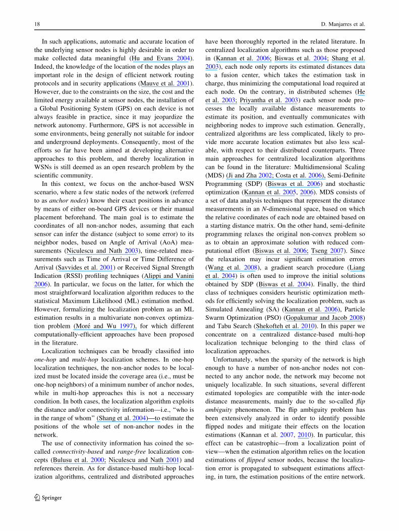
Figure 1 gives a glimpse of this concept: as the neighbors

of node A (i.e., nodes B, C, D, E) are nearly collinear, we

have that

dAB� dA0B; dAC � dA0C;

dAD� dA0D; dAE� dA0E:ð1Þ

It follows that node A can be reflected (flipped) with respect

to the virtual line connecting its neighbors to position A0,while satisfying the distance constraints and maintaining its

connectivity with anchor nodes C and E.

To alleviate this issue, an algorithm tackling the node

localization problem in presence of the flip ambiguity

phenomenon has been recently proposed in (Kannan et al.

2005). Basically, it consists of a two-phase optimization

scheme relying on Simulated Annealing (SA) for both

phases. In the first phase, SA is applied to obtain an initial

estimate of the node locations by minimizing the squared

error between the estimated and the measured inter-node

distances. In the second stage, a refinement phase first

identifies and then relocates the non-uniquely localizable

nodes which may have been flipped during the first stage,

by including an additional error term in the cost function,

when the estimated location of a node violates the con-

nectivity constraints defined by the network configuration.

Similarly, Gopakumar and Jacob in (Gopakumar and Jacob

2008) have proposed to apply a Particle Swarm Optimi-

zation (PSO) algorithm to tackle the problem, but, unlike

SA, they rely on a single execution of the PSO algorithm

and, instead of minimizing the sum of squared errors

between each non-anchor node and all its neighbors

(anchor and non-anchor nodes), they only take into account

those computed between each non-anchor node and its

neighboring anchor nodes. Thus, in sparser scenarios, as

the average node connectivity (and consequently the

anchor to non-anchor connectivity) decreases, the single-

hop PSO-based algorithm fails to obtain an accurate esti-

mation of the positions of the whole non-anchor nodes set.

This work joins the upsurge of research on meta-heu-

ristic centralized distance-based localization techniques.

Specifically, we propose to combine the Harmony Search

(HS) algorithm with a novel Local Search (LS) procedure

that aims at mitigating the flip ambiguity phenomenon

by exploiting the intrinsic connectivity constraints of the

network configuration. In particular, the localization

problem is formulated as the minimization of the sum of

two different, yet mutually related terms: the first repre-

sents the squared error between the estimated and the

measured inter-node distances, whereas the second estab-

lishes a penalty for all neighborhood violations in the

estimated network topology. Based on this rationale, our

proposal, hereafter referred to as HS-LS, can be regarded

as a centralized connectivity- and distance-based localiza-

tion approach with flipping mitigation. Extensive simula-

tions run over 12 different network topologies will

compare the performance of the proposed HS-LS with that

of the aforementioned meta-heuristic schemes proposed in

(Kannan et al. 2005; Gopakumar and Jacob 2008), as well

as with that of a Genetic Algorithm (GA) incorporating the

same local search procedure herein presented for a number

of different topologies and connectivity ranges. Results

will be discussed based on a number of statistics and

hypothesis tests utilized for assessing their statistical

significance.

This paper is organized as follows: in Sect. 2 the node

localization problem is formally posed, whereas Sect. 3

delves into the proposed HS-LS algorithm. Section 4

thoroughly describes the alternative meta-heuristics—the

algorithms in (Kannan et al. 2005; Gopakumar and Jacob

2008) and the implementation of a GA with the proposed

LS procedure—against which the proposed approach is

benchmarked. Next, Sect. 5 presents the simulation

framework and discusses the obtained experimental results

and finally, Sect. 6 concludes the paper.

2 Problem statement

We consider WSNs composed by n nodes uniformly

deployed in T � R2; from which m nodes (with m \ n)

correspond to the anchor nodes whose coordinates pi ¼ðxi; yiÞ 2 Tði 2 f1; . . .;mgÞ are perfectly known a priori.

The remaining n - m nodes are the non-anchor nodes,

whose positions pi ¼ ðxi; yiÞ; 8i 2 fmþ 1; . . .; ng are to be

estimated by the localization algorithm. We define an

n 9 n binary connectivity matrix C, such that cij = 1 if

sensor nodes i and j are within the connectivity range of

each other i.e., rij B R, where rij,jjpi � pjjj is the actual

distance between nodes i and j (k � k denotes the EuclideanFig. 1 Example of the flip ambiguity problem

Node localization in wireless sensor networks 19

123

norm) and R represents the circular transmission range,

common to all nodes. We further assume that each node

knows which nodes it can communicate with, thus this

information—embedded in matrix C—is a priori available.

The measured inter-node distances dij can be obtained by

resorting to any of the techniques introduced in Sect. 1, and

will be modeled as

dij ¼rij if ði; jÞ 2 f1; . . .;mg � f1; . . .;mg;

rij þ eij otherwise;

�ð2Þ

where rij stands for the actual inter-node distance between

node i and j, and eij represents the measurement error,

modeled as a Gaussian distributed random variable with

zero-mean and variance r2. Let us now define the set of

neighbors of node i as

N i, j 2 f1; . . .; ng; j 6¼ i : rij�R� �

; ð3Þ

and its complementary set N i; which contains the nodes

located outside the connectivity range of node i. Note that

the positions of the anchor nodes and the value of R

determine the regions in which each non-anchor node may

(or may not) be located. In particular, those non-anchor

nodes inside the coverage area of a certain anchor node

i 2 f1; . . .;mg should be placed in the circle of radius R

and centered in pi = (xi, yi), whereas the remaining non-

anchor nodes (i.e., those not connected to any anchor node)

should be located outside the union of the circles of radius

R and centered in all anchor nodes. Observe that this

information, roughly depending on R and {pi}i=1m , can be

exploited during the localization procedure to further refine

the position estimates of the non-anchor nodes.

With these definitions in mind, the objective of our

localization algorithm is to estimate the positions of all

non-anchor nodes by minimizing the sum1 of two objective

functions, labeled as CF (Cost Function) and SCV (Soft

Constraint Violation). CF simply represents the squared

error between the estimated and the measured inter-node

distances between nodes that are in the range of each other,

and can be defined as

CF,Xn

i¼mþ1

Xj2N i

ðdij � dijÞ20@

1A; ð4Þ

where dij and dij,

ffiffiffiffiffiffiffiffiffiffiffiffiffiffiffiffiffiffiffiffiffiffiffiffiffiffiffiffiffiffiffiffiffiffiffiffiffiffiffiffiffiffiffiðxi � xjÞ2 þ ðyi � yjÞ2

qrepresent the

measured and the estimated distances between node i and

its neighbor j, respectively. SCV takes into account the

connectivity neighborhood violations in each candidate

topology, acting as follows: if a node j has been placed in

the neighborhood of node i whilst j 2 N i or, alternatively,

its position is estimated such that dij [ R while j 2 N i;

then it is likely the node has been incorrectly placed: in

such situations, an error term ðdij � RÞ2 is added to SCV.2

Therefore, SCV can be formally defined as

SCV,Xn

i¼1

Xj2N i

dij [ R

ðdij � RÞ2 þXj2N i

dij �R

ðdij � RÞ2

0BBBB@

1CCCCA: ð5Þ

The defined SCV metric helps alleviating the flip

ambiguity phenomenon, especially in dense scenarios

where a local minimum in the CF metric may come

along with some connectivity violations in the estimated

topology. If so, an error term is added to the cost function

SCV, hence increasing the overall cost.

Finally, we evaluate the goodness of the estimated

topology by means of the Normalized Localization Error

(NLE), which is calculated as

NLE,100

R

ffiffiffiffiffiffiffiffiffiffiffiffiffiffiffiffiffiffiffiffiffiffiffiffiffiffiffiffiffiffiffiffiffiffiffiffiffiffiffiffiffiffiffiffiffiffiffiffi1

ðn� mÞXn

i¼mþ1

jjpi � pijj2s

: ½%� ð6Þ

It is important to emphasize that the computation of the

above defined NLE parameter requires the knowledge of

the real coordinates {pi}i=m?1n of non-anchor nodes, thus it

can not be regarded as an optimization metric, but instead

serves as a measure of the accuracy of the estimated

location solution fpigni¼mþ1:

3 Proposed HS-LS algorithm

To efficiently seek the optimum set of position estimates of

all non-anchor nodes, we propose to hybridize the well-

known heuristic HS algorithm with a novel local search

procedure that attempts at reducing the flipping ambiguities

in the candidate topology. As first presented by Geem,

Kim, and Loganathan in (Geem et al. 2001), the HS

algorithm belongs to the class of meta-heuristic population-

based stochastic search approaches, and is based on mim-

icking the improvisation process of musicians when jointly

composing a harmonious melody. This algorithm has been

widely used in several hard optimization instances framed

in distinct application fields, e.g. multicast routing (Forsati

et al. 2008), engineering design (Liao 2010), multiuser

detection (Zhang and Hanzo 2009; Gil-Lopez et al. 2009),

or radio resource allocation (Del Ser et al. 2010, 2011).

However, to the best of our knowledge, no previous work1 Unity-valued weights and no normalization have been considered in

the sum fitness, since the values of both constituent metrics result to

be in the same order of magnitude and thus, comparable for the

scenario at hand.

2 Indeed, it is worth to notice that the proposed error term represents

the minimum error due to a localization flip.

20 D. Manjarres et al.

123

has been reported in the scientific community dealing with

the application of HS to the node localization problem.

Let us elaborate further on the roots of the HS algorithm,

which in essence operates on a set of K candidate solutions

or melodies, which are referred to as Harmony Memory. In

our optimization framework, each melody encodes the

position of all nodes of the network, thus the Harmony

Memory can be denoted as ffpki g

ni¼1g

Kk¼1. The first m pairs

of real numbers represent the actual (x, y) positions of

anchor nodes (which, as said before, are assumed to be

perfectly known in advance), whereas the remaining n - m

pairs correspond to the estimated coordinates of all non-

anchor nodes of the network. Such K constituent melodies

are iteratively refined—in terms of their associated sum

metric CF ? SCV—by means of a stochastic improvisa-

tion process applied to every compounding element

fxki ; y

ki g

ni¼mþ1 of the candidate solution. Observe that this

stochastic improvisation procedure is only applied to the

estimated positions of non-anchor nodes, which are further

bounded by the topological constraints described in Sect. 2.

We also impose these constraints in the initialization phase

of the algorithm, where the starting candidate positions of

the non-anchor nodes in the Harmony Memory are drawn

at random from the areas defined by such topological

constraints. After the improvisation procedure, the value of

the sum metric function is computed for every improvised

melody, based on which the best K melodies—out of the

newly produced ones and those from the previous itera-

tion—are kept for the next iteration. This refinement is

repeated until a maximum number of iterations I is

reached. In the following, we will describe the steps and

the improvising operators used by our proposed HS-based

localization algorithm.

The proposed localization technique is sketched in

Algorithm 1, in pseudocode notation. There, the connec-

tivity radius R, the connectivity matrix C and the actual

positions of the m anchor nodes are provided as input

parameters to the algorithm. Moreover, a b ðmod cÞdenotes arithmetic congruence (i.e., a and b are congruent

modulo c if the difference (a - b) is an integer multiple of

c), whereas a:b (with a B b given integers) represents the

sequence fa; aþ 1; aþ 2; . . .; b� 1; bg: First, the esti-

mated positions of all nodes composing the Harmony

Memory (K 9 n-dimensional variable pEstimated) are

initialized at random (within the topological constraints).

Next, three different probabilistic operators are iteratively

applied (lines 8–10) to pEstimated so as to produce tenta-

tively refined candidate positions represented by the vari-

able p, namely:

– The Harmony Memory Considering Rate, HMCR 2½0; 1�; sets the probability that the new value for a

certain note ðxki ; y

ki Þ (i 2 fmþ 1; . . .; ng) is drawn

uniformly from the values of the same note in all the

other K - 1 melodies in the Harmony Memory (HM).

– The Pitch Adjusting Rate, PAR 2 ½0; 1�; establishes the

probability that the new value for a given note ðxki ; y

ki Þ

(again, i 2 fmþ 1; . . .; ng) is randomly taken from its

coverage area considering the geometrical constraints

imposed by the anchor nodes for the non-anchor node

at hand.

– The probability to pick a random value for the new note

ðxki ; y

ki Þ is controlled by another probabilistic parameter

RSR (Random Selection Rate) 2 ½0; 1�: As opposed to

the PAR procedure, the RSR parameter operates

network-wide along the subset Ti � T ¼ ½0; 1� � ½0; 1�;which is defined by the intersection of all geometrical

constraints established by the connectivity range of the

anchor nodes.

Once the operators have been applied to 8i 2 fmþ1; . . .; ng; the algorithm checks whether the notes of

every newly improvised candidate coordinates of the

Harmony Memory are within the network boundaries and

eventually modifies such values to the closer boundary of

T (line 11).

The proposed approach proceeds by performing a local

search procedure every ILS iterations. This procedure aims

at improving the fitness value of the improvised candidate

with potentially lowest metric value and is applied to each

non-anchor node lying outside the connectivity range of

any anchor node and whose any of its neighbors in the

estimated topology differs from those imposed by the

Algorithm 1 Algorithmic description of the proposed HS-based

localization approach

Node localization in wireless sensor networks 21

123

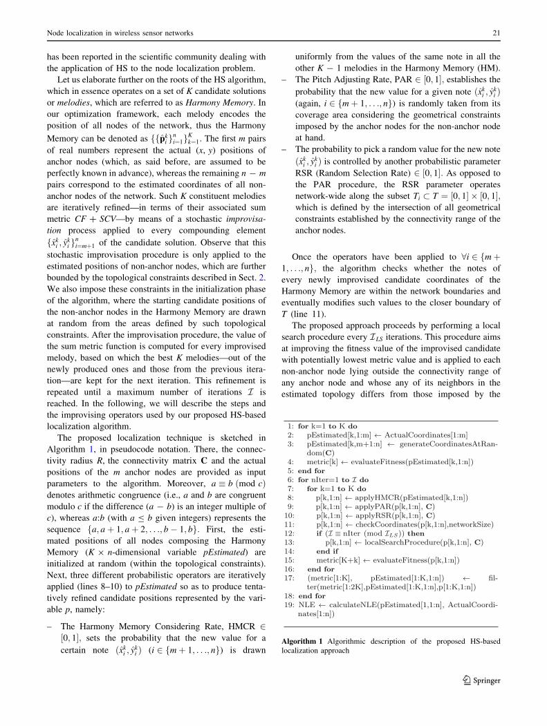
connectivity matrix C. Figure 2a, b depict an example of

the application of the local search procedure to the esti-

mated node 30 in a simplistic setup. In this scenario, the

following notation is adopted: the anchor nodes are rep-

resented with crosses (9), whereas the actual non-anchor

nodes are marked as circles (• for the actual node 3, � for

its actual neighbors 4, 5, 6 and 7) and the corresponding

estimated coordinates as squares (j for the estimated node

30, h for its estimated neighbor nodes 40, 50, 60, 70, 80 and

90). Given that there are false neighbors in the estimated

network topology violating the connectivity constraints

imposed by C (i.e., 80 and 90), the proposed local search

procedure is applied by sequentially executing the fol-

lowing steps:

1. Selection of a non-anchor node lying outside the

connectivity range of any anchor node and whose

neighbors in the estimated topology differs from those

imposed by C, i.e., node 30.2. Creation of the set of nodes that are going to be moved

together with node 30: this group is filled with the non-

anchor nodes that are not connected to any anchor

node and are within the connectivity range of node 3 in

the actual topology. In our case, since c3j = 1 only for

j 2 f4; 5; 6; 7g; nodes 1 and 2 are anchor nodes and

c16 = c24 = 1, this set is composed by nodes 50 and 70.3. Identification of the anchor nodes located within the

connectivity range of the actual neighbors of node 3; in

our setup, nodes 1 and 2.

4. Move the node at hand (node 30) to the intersection of

the annuli with inner and outer radii R and 2R respec-

tively, centered in the selected anchor nodes 1 and 2,

under the condition that the number of false neighbors

decreases.

5. Place the actual neighbors, which are not connected to

any anchor (i.e., nodes 50 and 70), randomly inside the

circular coverage region centered in the new location

of node 30 (see Fig. 2b).

The new generated candidate solutions are then eval-

uated (line 15) and the Harmony Memory is updated

based on the global metric function CF ? SCV (line 17).

To this end, only those K harmonies improving the fitness

with respect to those from the previous iteration are

included in the next Harmony Memory. Once this has

been done, the harmony memory is sorted in ascending

order of the fitness values of its compounding melodies.

Consequently, the potentially best candidate topology

within a certain iteration will be given by pEstimat-

ed[1,1:n]. This procedure is repeated until a fixed number

of iterations I is achieved and finally, the NLE value is

computed in line 19 in order to assess the quality of the

final estimate.

4 Related approaches

In this section we summarize different approaches pre-

sented in the literature for solving the node localization

problem. Such schemes will be later used for assessing the

performance of our proposed algorithm with respect to the

state of the art in meta-heuristic localization in wireless

sensor networks.

First, let us delve into the SA-based localization method

presented in (Kannan et al. 2006). SA is essentially a sto-

chastic optimization algorithm inspired by the physical

process of annealing in metallurgy. As opposed to gradient-

based search methods which employ the idea of steepest

descent at each iteration, SA allows random uphill per-

turbations, thus preventing the search process from getting

stuck in local minima by accepting worse candidate solu-

tions based on probabilistic parameters. The specific SA

localization approach in (Kannan et al. 2006) performs a

two-stage optimization procedure: in the first phase, a

preliminary estimate of the positions of non-anchor nodes

is obtained by minimizing the CF objective function as

defined in Eq. (4). This minimization is accomplished by

executing a first instance of the SA algorithm for a given

(a)

(b)

Fig. 2 a Example of a scenario to which the local search procedure is

applied; b resulting candidate topology after applying the local search

procedure

22 D. Manjarres et al.

123

number of iterations set beforehand. At the end of the first

stage, the non-anchor nodes fulfilling all the connectivity

constraints imposed by matrix C are identified and elevated

to the status of virtual anchor nodes, whilst the remaining

nodes (i.e., those non-anchor nodes undergoing the afore-

mentioned flipping ambiguity) are relocated during the

second refinement round of SA which minimizes a new

cost function defined as

CFSA,

Xn

i¼mþ1

Xj2Ni

ðdij�dijÞ2 þXj2Ni

dij �R

ðdij�RÞ2

0BBB@

1CCCA: ð7Þ

The pseudocode of the SA-based algorithm is shown in

Algorithm 2. First, the control temperature Tc is set at a

high value to perform a highly explorative random search

within the solution space of the problem. At each iteration,

the control temperature Tc is decreased from T0 to Tf

according to line 26 (with a\ 1), whereas the distance gap

DD is also set decreasing from its starting value DD0 at a

rate b\ 1 (line 27). On the other hand, N � P� Q

randomly selected non-anchor nodes are perturbed (with

N, n� m; and P and Q being design parameters). Each

perturbed topology is then evaluated and accepted if it is

characterized by a better fitness value with respect to the

current one (lines 11–15). Otherwise, the solution with

a worse fitness value is accepted with a probability

expf�DCFTcg (lines 16–20), where DCF represents the

difference between the current and previous values of the

metric function. The control temperature Tc, which drives

the acceptance rate of worse candidate estimates, cools

down as the number of iterations increases.

On the other hand, the authors in (Gopakumar and Jacob

2008) proposed a PSO-based localization algorithm for

WSNs. Unlike SA, PSO is inspired by the social behaviors

and movement patterns of bird flocks or fish schools. Each

particle’s movement is influenced by its best location esti-

mate and the global estimate of the whole set of particles.

Following the notation in (Gopakumar and Jacob 2008) and

assuming a 2-dimensional localization scenario, let

pbestk,ðpbestxk; pbesty

kÞðpersonal bestÞ

denote the best position vector attained by the k-th particle

during the search procedure, and let gbest,ðgbestx; gbestyÞrepresent the position of the global best particle in the

K-dimensional particle swarm, i.e., the particle with the

lowest metric function value. At the i-th iteration of the

algorithm, the particles’ velocities fvk;igKk¼1,fðvx

k;i; vyk;iÞg

Kk¼1

and the estimated position vector fpk;igKk¼1,fðpx

k;i; pyk;iÞg

Kk¼1

of all particles are updated according to

vwk;i ¼ xvw

k;i�1 þ c1r1ðpbestwk � pwk;i�1Þ

þ c2r2ðgbestw � pwk;i�1Þ;

ð8Þ

pwi ¼ pw

i�1 þ vwi ; ð9Þ

Algorithm 2 The SA approach

proposed in (Kannan et al.

2006)

Node localization in wireless sensor networks 23

123

where w 2 fx; yg; r1 and r2 represents random numbers 2½0; 1�;w refers to the inertial weight and c1 and c2 are

known as cognitive and social scaling parameters,

respectively. The fitness function to be minimized by the

proposed PSO algorithm is set to

CFPSO,

XN

j¼1

1

N !j

XN !j

i¼1

ðffiffiffiffiffiffiffiffiffiffiffiffiffiffiffiffiffiffiffiffiffiffiffiffiffiffiffiffiffiffiffiffiffiffiffiffiðx�xiÞ2 þ ðy�yiÞ2

q� diÞ2; ð10Þ

where di corresponds to the noisy measured distance

between the non-anchor node to be localized and its

neighboring anchor nodes; N!j is the number of neighbor-

ing anchor nodes of node j; (xi, yi) are the coordinates of

anchor nodes and (x, y) the coordinates of the target node

to be estimated. It is important to note that the authors

in (Gopakumar and Jacob 2008) explicitly impose that

N !j 38j; since no further mechanism is incorporated to

the proposed PSO approach in order to account for possible

flipping ambiguities. Nevertheless, we will use this single-

hop algorithm in our benchmark so as to evince the

importance of reducing the flip ambiguity phenomenon in

sparse scenarios.

Finally, the meta-heuristics utilized for comparison in

the next Section include a naive implementation of a

population-based GA minimizing CF ? SCV by exploiting

classical uniform crossover and uniform mutation as mat-

ing operators (with probability Pc and Pm, respectively),

together with the same LS procedure described in Sect. 3.

5 Simulation results

In order to assess the effectiveness of the proposed HS-LS

algorithm when tackling the localization problem in WSNs,

we have performed a number of computer simulations over

synthetic networks with different levels of sparsity. In

order to compare its performance against the previously

mentioned soft-computing localization techniques, we have

executed the PSO algorithm formulated in (Gopakumar

and Jacob 2008) and the SA-based scheme proposed in

(Kannan et al. 2006) over the same scenarios. Likewise, for

the sake of completeness we also have included a naive

implementation of a standard GA incorporating the local

search procedure previously described (Sect. 3).

The simulation framework consists of 12 different net-

work topologies generated by uniformly placing n = 200

nodes in T , ½0; 1� � ½0; 1�: In all such topologies, m = 20

nodes are set as anchor nodes, hence their positions are

assumed to be known a priori and fed to the algorithms.

Moreover, we have varied the connectivity radius R 2f0:13; 0:15; 0:17g; so as to model 3 different network sparsity

levels, each composed by 4 topologies. In particular, TOP1 to

TOP4 represent the sparse topologies class (R = 0.13);

TOP5 to TOP8 constitute the class of medium-sparse topol-

ogies (R = 0.15); and TOP9 to TOP12 form the class of

dense topologies (R = 0.17). Finally, the inter-sensor dis-

tance measurements (2) are assumed to be based on RSSI,

which is commonly affected by log-normal shadowing with

standard deviation of the errors proportional to the actual

distance rij between nodes i and j (Liu et al. 1998). Without

loss of generality, in the following and for all the scenarios,

the measurement errors eij are considered constant through all

experiments for a given topology, with values drawn from a

Gaussian distribution with zero mean and variance given by

r2 ¼ k2 � r2ij; with k = 0.1.

Table 1 summarizes the parameters setup employed by

the different algorithms and deriving from a preliminary

simulation campaign conducted to choose the most effec-

tive configurations. For the sake of the brevity, this pre-

liminary analysis is omitted.

First, with the goal of analyzing the computational

complexity, it is worth to characterize each approach in

terms of required number of fitness evaluations. On the one

hand, HS-LS and GA-LS employs a fixed number I ¼2;000 of iterations while, at each iteration, the objective

function is evaluated K = 50 times (one for each newly

generated candidate solution). Therefore, in each trial the

overall number of fitness evaluations for both the algo-

rithms is equal to K � I ¼ 105: Moreover, in these algo-

rithms the local search procedure LS is applied to the best

candidate topology every ILS ¼ 100 iterations. Regarding

the PSO scheme (Gopakumar and Jacob 2008), a swarm

size of K = 100 particles is evaluated during I ¼ 2000

iterations. It follows that, in each trial, PSO performs K �I ¼ 2� 105 fitness evaluations. Finally, the number of

fitness evaluations performed by SA (Kannan et al. 2006)

at each value of the control temperature, during the first

optimization phase is equal to ðn� mÞ � P� Q: Unfortu-

nately, the number of fitness evaluations performed during

the refinement phase cannot be determined in advance,

as the number of non-anchor nodes promoted to virtual

Table 1 Parameters setup used for the PSO, SA, GA-LS and HS-LS

algorithms

PSO SA GA-LS HS-LS

Tc,i: 0.1

w: [0.8, 0.7] Tc,f: 10-11 Pc: 0.9 HMCR: 0.9

c1: [0.8, 0.6] P: 10 Pm: 0.01 PAR: 0.01

c2: [0.8, 0.6] Q: 2 K: 50 RSR: 0.01

K: 100 a: 0.80 I : 2000 K: 50

I : 2000 b: 0.94 ILS : 100 I : 2000

DD0 : 0:1 ILS : 100

24 D. Manjarres et al.

123

anchor nodes is variable. However, we have verified that

SA computes, on average, around 7:1� 105 fitness evalu-

ations during each trial. Thus, HS-LS and GA-LS reduce

the computational load with respect to the PSO and SA

counterparts in approximately 2:1 and 7:1 ratios, respec-

tively. We remark that the rationale of selecting configu-

rations with different complexity levels lies on the

aforementioned preliminary off-line campaign, during

which we could verify that, by using the parameters setup

resumed in Table 1, the simulation results of each

algorithm become stationary and/or comparable (in terms

of the same order of magnitude in the results).

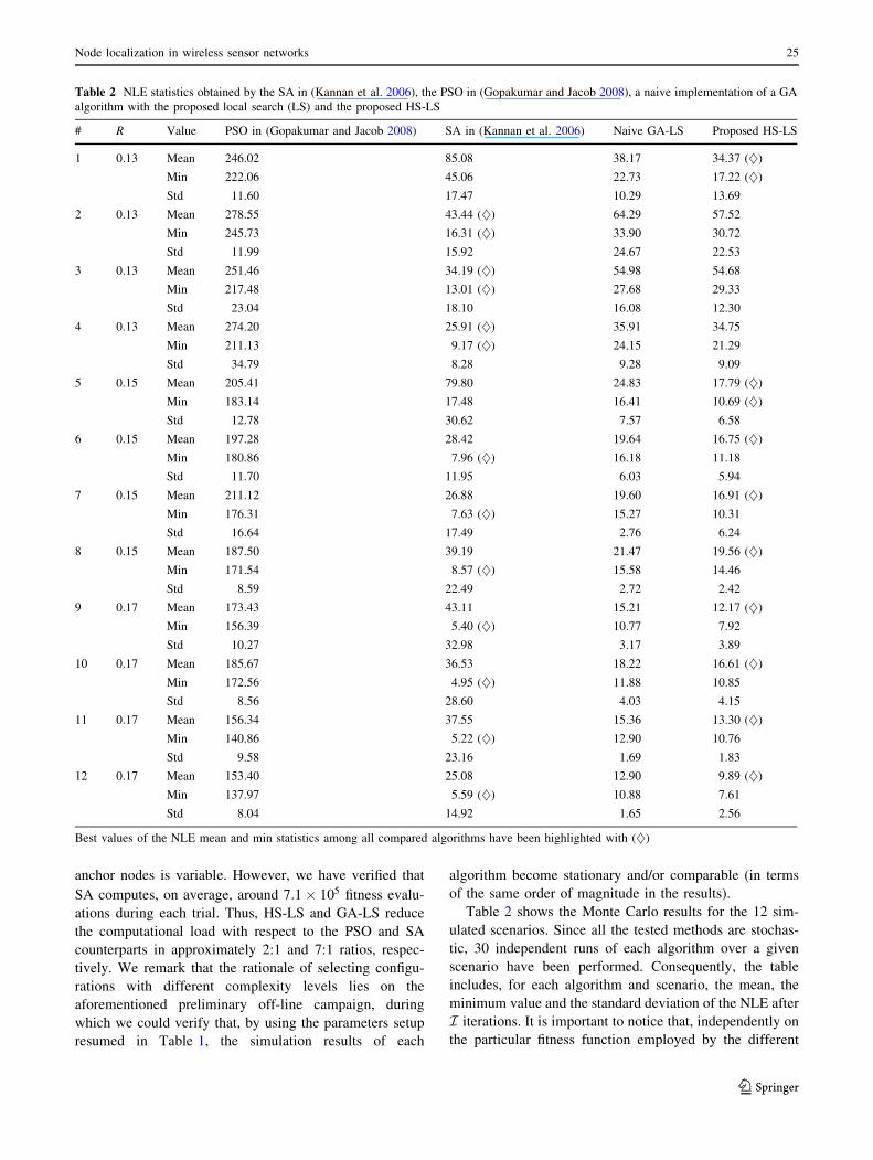
Table 2 shows the Monte Carlo results for the 12 sim-

ulated scenarios. Since all the tested methods are stochas-

tic, 30 independent runs of each algorithm over a given

scenario have been performed. Consequently, the table

includes, for each algorithm and scenario, the mean, the

minimum value and the standard deviation of the NLE after

I iterations. It is important to notice that, independently on

the particular fitness function employed by the different

Table 2 NLE statistics obtained by the SA in (Kannan et al. 2006), the PSO in (Gopakumar and Jacob 2008), a naive implementation of a GA

algorithm with the proposed local search (LS) and the proposed HS-LS

# R Value PSO in (Gopakumar and Jacob 2008) SA in (Kannan et al. 2006) Naive GA-LS Proposed HS-LS

1 0.13 Mean 246.02 85.08 38.17 34.37 (})

Min 222.06 45.06 22.73 17.22 (})

Std 11.60 17.47 10.29 13.69

2 0.13 Mean 278.55 43.44 (}) 64.29 57.52

Min 245.73 16.31 (}) 33.90 30.72

Std 11.99 15.92 24.67 22.53

3 0.13 Mean 251.46 34.19 (}) 54.98 54.68

Min 217.48 13.01 (}) 27.68 29.33

Std 23.04 18.10 16.08 12.30

4 0.13 Mean 274.20 25.91 (}) 35.91 34.75

Min 211.13 9.17 (}) 24.15 21.29

Std 34.79 8.28 9.28 9.09

5 0.15 Mean 205.41 79.80 24.83 17.79 (})

Min 183.14 17.48 16.41 10.69 (})

Std 12.78 30.62 7.57 6.58

6 0.15 Mean 197.28 28.42 19.64 16.75 (})

Min 180.86 7.96 (}) 16.18 11.18

Std 11.70 11.95 6.03 5.94

7 0.15 Mean 211.12 26.88 19.60 16.91 (})

Min 176.31 7.63 (}) 15.27 10.31

Std 16.64 17.49 2.76 6.24

8 0.15 Mean 187.50 39.19 21.47 19.56 (})

Min 171.54 8.57 (}) 15.58 14.46

Std 8.59 22.49 2.72 2.42

9 0.17 Mean 173.43 43.11 15.21 12.17 (})

Min 156.39 5.40 (}) 10.77 7.92

Std 10.27 32.98 3.17 3.89

10 0.17 Mean 185.67 36.53 18.22 16.61 (})

Min 172.56 4.95 (}) 11.88 10.85

Std 8.56 28.60 4.03 4.15

11 0.17 Mean 156.34 37.55 15.36 13.30 (})

Min 140.86 5.22 (}) 12.90 10.76

Std 9.58 23.16 1.69 1.83

12 0.17 Mean 153.40 25.08 12.90 9.89 (})

Min 137.97 5.59 (}) 10.88 7.61

Std 8.04 14.92 1.65 2.56

Best values of the NLE mean and min statistics among all compared algorithms have been highlighted with (})

Node localization in wireless sensor networks 25

123

stochastic algorithms to explore the solution space, the

NLE indicator (6) enables a fair comparison among the

approaches. Indeed, it represents the deviation of an esti-

mation of the sensor nodes’ locations with respect to the

real topology, normalized by the connectivity radius. Thus,

assuming that the estimate is unbiased, the NLE can be

interpreted as the ratio of the standard deviation to the

connectivity radius. As aforementioned in Sect. 2 note that,

being the original topology unknown, the NLE cannot be

directly employed as fitness function during the search

phase, while it can be employed as an a posteriori, yet

objective, quality assessment indicator. First observe that

the mean and the standard deviation of the NLE obtained

by the HS-LS localization approach are in general lower

than those achieved by the SA and the PSO algorithms, and

similar (but still better than) to those obtained by the GA-

LS scheme. On the other hand, the best (minimum) NLE

values are in general lower for the SA—though it needs 7

times more function evaluations than its GA-LS and HS-LS

counterparts—similar for the GA-LS and HS-LS schemes,

but significantly higher for the PSO technique.

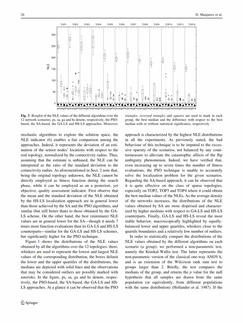
Figure 3 shows the distributions of the NLE values

obtained by all the algorithms over the 12 topologies: there,

whiskers are used to represent the lowest and largest NLE

values of the corresponding distribution, the boxes delimit

the lower and the upper quartiles of the distributions, the

medians are depicted with solid lines and the observations

that may be considered outliers are possibly marked with

asterisks. In the figure, ps, sa, ga and hs denote, respec-

tively, the PSO-based, the SA-based, the GA-LS and HS-

LS approaches. At a glance it can be observed that the PSO

approach is characterized by the highest NLE distributions

in all the experiments. As previously stated, the bad

behaviour of this technique is to be imputed to the exces-

sive sparsity of the scenarios, not balanced by any coun-

termeasure to alleviate the catastrophic affects of the flip

ambiguity phenomenon. Indeed, we have verified that,

even increasing up to seven times the number of fitness

evaluations, the PSO technique is unable to accurately

solve the localization problem for the given scenarios.

Regarding the SA-based approach, it can be observed that

it is quite effective on the class of sparse topologies,

especially on TOP2, TOP3 and TOP4 where it could obtain

the best median values of the NLEs. As the average density

of the networks increases, the distributions of the NLE

values obtained by SA are more dispersed and character-

ized by higher medians with respect to GA-LS and HS-LS

counterparts. Finally, GA-LS and HS-LS reveal the most

stable behavior, macroscopically highlighted by equally-

balanced lower and upper quartiles, whiskers close to the

quartile boundaries and a relatively low number of outliers.

In order to statistically compare the distributions of the

NLE values obtained by the different algorithms on each

scenario (a group), we performed a non-parametric test,

namely the Kruskal-Wallis test. The latter represents the

non-parametric version of the classical one-way ANOVA,

and is an extension of the Wilcoxon rank sum test to

groups larger than 2. Briefly, the test compares the

medians of the group, and returns the p value for the null

hypothesis that all samples are drawn from the same

population (or equivalently, from different populations

with the same distribution) (Hollander et al. 1987). If the

Fig. 3 Boxplot of the NLE values of the different algorithms over the

12 network scenarios. ps, sa, ga and hs denote, respectively, the PSO-

based, the SA-based, the GA-LS and HS-LS approaches. Moreover,

triangles, reversed triangles and squares are used to mark in each

group, the best median and the difference with respect to the best

median with or without statistical significance, respectively

26 D. Manjarres et al.

123

p value is lower than a, we can deduce that the null

hypothesis does not hold, that is, at least one sample

median in the group is significantly different from the

others, with (1 - a) percent level of confidence. Then, to

determine which sample medians are statistically differ-

ent, we have applied the multiple comparison procedure

with a = 0.05 (thus, with a 95% level of confidence)

(Hochberg and Tamhane 1987). The results of such pro-

cedure are depicted in Fig. 3, by means of triangles (m),

reversed triangles (.) and squares (j). In detail, within

each group, a triangle marks the distribution with the best

median (i.e., the lowest), while a reversed triangle and

square mean, respectively, that the median of the corre-

sponding distribution is larger than the best median of the

group with or without statistical significance. We can

observe in this plot that HS-LS produces the best NLEs

results over 9 scenarios (all except TOP2, TOP3 and

TOP4). In the remaining scenarios, SA achieves the best

results, but with statistical significance with respect to HS-

LS only in one scenario (TOP3). Finally, GA-LS, though

quite stable and effective, could never obtain the best

median, while its worse results with respect to the best

median distribution have a statistical significance in 5

scenarios (TOP2, TOP3, TOP4, TOP7 and TOP12).

6 Concluding remarks

In this paper we have presented a novel meta-heuristic

localization technique for wireless sensor networks based on

the harmony search algorithm, which is further aided by a

local search procedure aiming at alleviating the so-called flip

ambiguity phenomenon. The proposed algorithm exploits the

information on the node connectivity by imposing geomet-

rical constraints in order to restrain the areas where sensor

nodes can be placed. Through extensive computer simula-

tions, we have shown that our approach embodies a cost-

effective centralized localization scheme outperforming, for

most of the simulated scenarios, other recently proposed

meta-heuristic strategies such as SA, PSO and a naive GA

incorporating the local search procedure here presented.

Acknowledgments This work has been supported in part by the

Spanish Ministry of Science and Innovation through the CONSOL-

IDER-INGENIO 2010 (CSD200800010) and the Torres-Quevedo

(PTQ-09-01-00740) funding programs.

References

Akyildiz IF, Su W, Sankarasubramaniam Y, Cayirci E (2002)

Wireless sensor networks: a survey. Comput Netw 38:393–422

Alippi C, Vanini G (2006) A RSSI-based and calibrated centralized

localization technique for wireless sensor networks. In: Pro-

ceedings of fourth IEEE international conference on pervasive

computing and communications workshops, pp 301–305

Biswas P, Liang TC, Toh KC, Ye Y, Wang TC (2006) Semidefinite

programming approaches for sensor network localization with

noisy distance measurements. IEEE Trans Automat Sci Eng

3(4):360–371

Biswas P, Ye Y (2004) Semidefinite programming for ad-hoc wireless

sensor network localization. In: Proceedings of the 3rd interna-

tional symposium on information processing in sensor networks.

ACM Press, New York, pp 46–54

Bulusu N, Heidemann J, Estrin D (2000) GPS-less Low-cost outdoor

localization for very small devices. IEEE Personal Commun

7(5):28–34

Costa JA, Patwari N, Hero AO (2006) Distributed weighted-

multidimensional scaling for node localization in sensor net-

works. ACM Trans Sens Netw 2:1

Del Ser J, Matinmikko M, Gil-Lopez S, Mustonen M (2010) A novel

harmony search based spectrum allocation technique for cogni-

tive radio networks. IEEE international symposium on wireless

communication systems, pp 233–237

Del Ser J, Bilbao MN, Gil-Lopez S, Matinmikko M, Salcedo-Sanz S

(2011) Iterative power and subcarrier allocation in rate-con-

strained orthogonal multicarrier downlink systems based on

hybrid harmony search heuristics. Eng Appl Artif Intell 24(5):

748–756

Forsati R, Haghighat AT, Mahdavi M (2008) Harmony search based

algorithms for bandwidth-delay-constrained least-cost multicast

routing. Comput Commun 31(10):2505–2519

Geem ZW, Kim JH, Loganathan GV (2001) A new heuristic

optimization algorithm: harmony search. Simulation 76(2):60–

68

Gil-Lopez S, Del Ser J, Olabarrieta I (2009) A novel heuristic

algorithm for multiuser detection in synchronous cdma wireless

sensor networks. IEEE international conference on ultra modern

communications, pp 1–6

Gopakumar A, Jacob L (2008) Localization in wireless sensor

network using particle swarm optimization. IET international

conference on wireless, mobile and multimedia networks,

pp 227–230

He T, Huang C, Blum B, Stankovic J, Abdelzaher T (2003) Range-

free localization schemes in large scale sensor network. In:

Proceedings of the ninth annual international conference on

mobile computing and networking, pp 81–95

Hochberg Y, Tamhane AC (1987) Multiple comparison procedures.

Wiley, New York

Hollander M, Wolfe DA (1973) Nonparametric statistical methods.

Wiley, New York

Hu L, Evans D (2004) Localization for Mobile Sensor Networks.

Proceedings of the 10th International Conference on Mobile

Computing and Networking, pp 45–57

Ji X, Zha H (2004) Sensor positioning in wireless ad-hoc sensor

networks using multidimensional scaling. In: Proceedings of the

23rd annual joint conference of the IEEE computer and

communications societies, pp 2652–2661

Kannan AA, Fidan B, Mao G, Anderson BDO (2007) Analysis of flip

ambiguities in distributed network localization. information,

decision and control, pp 193–198

Kannan AA, Fidan B, Mao G (2010) Analysis of flip ambiguities for

robust sensor network localization. IEEE Trans Veh Technol

59(4):2057–2070

Kannan AA, Mao G, Vucetic B (2005) Simulated annealing based

localization in wireless sensor network. In: Proceedings of the

IEEE conference on local computer networks. IEEE Computer

Society, pp 513–514

Kannan AA, Mao G, Vucetic B (2006) Simulated annealing based

wireless sensor network localization with flip ambiguity mitiga-

tion. In: Proceedings of the 63-rd IEEE vehicular technology

conference 1022–1026

Node localization in wireless sensor networks 27

123

Liang TC, Wang TC, Ye Y (2004) A Gradient Search Method to

Round the Semidefinite Programming Relaxation for Ad Hoc

Wireless Sensor Network Localization. Standford University

Technical Report

Liao TW (2010) Two hybrid differential evolution algorithms for

engineering design optimization. Appl Soft Comput 10(4):1188–

1199

Liu T, Bahl P, Chlamtac I (1998) Mobility modeling, location

tracking, and trajectory prediction in wireless ATM networks.

IEEE J Sel Areas Commun 16(6):922–936

Mauve M, Widmer J, Hartenstein H (2001) A survey on position-

based routing in mobile adhHoc networks. IEEE Netw 15(6):30–

39

More JJ, Wu Z (1997) Global continuation for distance geometry

problems. SIAM J Optimiz 7(3):814–836

Niculescu D, Nath B (2001) Ad hoc positioning system (APS). IEEE

global communications conference (GLOBECOM) 5:2926–2931

Niculescu D, Nath B (2003) Ad-hoc positioning system (APS) using

AoA. In: Proceedings of the 20st annual joint conference of the

IEEE computer and communications societies 3:1734–1743

Priyantha N, Balakrishnan H, Demaine E, Teller S (2003) Anchor-

free distributed localization in sensor network. MIT Laboratory

for Computer Science TR-892

Savvides A, Han CC, Srivastava M (2001) Dynamic fine-grained

localization in ad-hoc networks of sensors. In: 7th ACM

international conference on mobile computing and networking,

pp 166–179

Shang Y, Ruml W, Zhang Y, Fromherz M (2003) Localization from

mere connectivity. In: Proceedings of ACM symposium on

mobile ad hoc networking and computing, pp 201–212

Shang Y, Ruml W, Zhang Y, Fromherz M (2004) Localization from

Connectivity in Sensor Networks. IEEE Trans Parallel Distrib-

uted Syst 15(11):961–974

Shekofteh SK, Khalkhali MB, Yaghmaee MH, Deldari H (2010)

Localization in Wireless Sensor Networks using Tabu Search

and Simulated Annealing. In: 2nd international conference on

computer and automation engineering (ICCAE) 2:752–757

Tseng P (2007) Second-order cone programming relaxation of sensor

network localization. SIAM J Optim 18(1):156–185

Wang Z, Zheng S, Ye Y, Boyd S (2008) Further relaxations of the

semidefinite programming approach to sensor network localiza-

tion. SIAM J Optim 19(2):655–673

Zhang R, Hanzo L (2009) Iterative multiuser detection and channel

decoding for DS-CDMA using harmony search. IEEE Signal

Process Lett 16(10):917–920

28 D. Manjarres et al.

123