Research Article A Novel Bearing Fault Diagnosis Methodology Based on SVD and One-Dimensional Convolutional Neural Network Yangyang Wang , 1 Shuzhan Huang , 2 Juying Dai , 3 and Jian Tang 3 1 Xichang Satellite Launch Center, Xichang 615000, China 2 School of Graduate, Army Engineering University of PLA, Nanjing 210000, China 3 School of Field Engineering, Army Engineering University of PLA, Nanjing 21000, China Correspondence should be addressed to Shuzhan Huang; [email protected] Received 12 June 2019; Revised 16 October 2019; Accepted 12 December 2019; Published 30 January 2020 Academic Editor: Salvatore Russo Copyright © 2020 Yangyang Wang et al. is is an open access article distributed under the Creative Commons Attribution License, which permits unrestricted use, distribution, and reproduction in any medium, provided the original work is properly cited. is paper constructs a novel network structure (SVD-1DCNN) based on singular value decomposition (SVD) and one-di- mensional convolutional neural network (1DCNN), which takes the original signal as input to realize intelligent diagnosis of bearing faults. e output of the first convolution layer was also analyzed from the perspectives of time domain and time- frequency domain in the simulation experiment. rough qualitative analysis and quantitative analysis, it was found that the convolution kernel not only extracted the classification features of signals but also gradually highlighted the learned features in the network training process. Moreover, applying this network in fault diagnosis of bearing date provided by the Case Western Reserve University (CWRU) Bearing Data Center, it was found that the convolution kernel could also achieve the above operation. e novel network of this paper achieved a good classification effect on both the simulated signals and the measured signals. 1. Introduction A small fault in a mechanical device often affects the stability and safety of the entire system and can even lead to cata- strophic consequences [1]. As a key component of me- chanical equipment, bearings are widely used in various types of machinery. Failure of the bearing can cause many serious mechanical failures, so the safe and smooth oper- ation of the bearing is critical to the mechanical equipment. Timely detection, positioning, and troubleshooting of bearing faults can effectively improve the safety of industrial production. erefore, it is of great significance to study the fault diagnosis of bearing. e traditional fault diagnosis process generally consists of three steps: data acquisition, feature extraction and se- lection, and fault pattern recognition [2]. e collected data include vibration signal, acoustic signal, and temperature signal, and since the vibration signal can directly characterize the state of the mechanical equipment, the vibration signal is most commonly collected in fault diagnosis [3]. In the fault diagnosis of bearing, commonly used signal processing methods include Fourier transform (FT) [4], short-time Fourier transform (STFT) [5], wavelet transform (WT) [6], Wigner–Ville distribution (WVD) [7], and empirical mode decomposition (EMD) [8]. e above methods can extract features that are conducive for classification and diagnosis [9, 10] and then pass the extracted features through various classifiers to realize pattern recognition of bearing faults. Among the various pattern recognition methods, the machine learning-based method is the most used. Wang et al. [11] used KPCA to extract features from bearing fault signal and used k-nearest neighbor (KNN) as a classifier to achieve diagnosis; Fei et al. [12] reconstructed the characteristics of bearing vibration signal after singular value decomposition based on wavelet packet transform phase space and established support vector machine (SVM) model of bearing diagnosis; Mahamad and Hiyama [13] performed fast Fourier transform (FFT) and envelope processing on the bearing vibration signal, extracted time domain and frequency domain feature as input, and then used ANN to fulfill the diagnosis. However, the existing intelligent fault diagnosis methods based on the Hindawi Shock and Vibration Volume 2020, Article ID 1850286, 17 pages https://doi.org/10.1155/2020/1850286

Welcome message from author
This document is posted to help you gain knowledge. Please leave a comment to let me know what you think about it! Share it to your friends and learn new things together.
Transcript

Research ArticleA Novel Bearing Fault Diagnosis Methodology Based on SVD andOne-Dimensional Convolutional Neural Network
Yangyang Wang 1 Shuzhan Huang 2 Juying Dai 3 and Jian Tang 3
1Xichang Satellite Launch Center Xichang 615000 China2School of Graduate Army Engineering University of PLA Nanjing 210000 China3School of Field Engineering Army Engineering University of PLA Nanjing 21000 China
Correspondence should be addressed to Shuzhan Huang hsz_221618163com
Received 12 June 2019 Revised 16 October 2019 Accepted 12 December 2019 Published 30 January 2020
Academic Editor Salvatore Russo
Copyright copy 2020 YangyangWang et al -is is an open access article distributed under the Creative Commons Attribution Licensewhich permits unrestricted use distribution and reproduction in any medium provided the original work is properly cited
-is paper constructs a novel network structure (SVD-1DCNN) based on singular value decomposition (SVD) and one-di-mensional convolutional neural network (1DCNN) which takes the original signal as input to realize intelligent diagnosis ofbearing faults -e output of the first convolution layer was also analyzed from the perspectives of time domain and time-frequency domain in the simulation experiment -rough qualitative analysis and quantitative analysis it was found that theconvolution kernel not only extracted the classification features of signals but also gradually highlighted the learned features in thenetwork training process Moreover applying this network in fault diagnosis of bearing date provided by the Case WesternReserve University (CWRU) Bearing Data Center it was found that the convolution kernel could also achieve the above operation-e novel network of this paper achieved a good classification effect on both the simulated signals and the measured signals
1 Introduction
A small fault in a mechanical device often affects the stabilityand safety of the entire system and can even lead to cata-strophic consequences [1] As a key component of me-chanical equipment bearings are widely used in varioustypes of machinery Failure of the bearing can cause manyserious mechanical failures so the safe and smooth oper-ation of the bearing is critical to the mechanical equipmentTimely detection positioning and troubleshooting ofbearing faults can effectively improve the safety of industrialproduction -erefore it is of great significance to study thefault diagnosis of bearing
-e traditional fault diagnosis process generally consistsof three steps data acquisition feature extraction and se-lection and fault pattern recognition [2]
-e collected data include vibration signal acousticsignal and temperature signal and since the vibration signalcan directly characterize the state of the mechanicalequipment the vibration signal is most commonly collectedin fault diagnosis [3] In the fault diagnosis of bearing
commonly used signal processing methods include Fouriertransform (FT) [4] short-time Fourier transform (STFT)[5] wavelet transform (WT) [6] WignerndashVille distribution(WVD) [7] and empirical mode decomposition (EMD) [8]-e above methods can extract features that are conducivefor classification and diagnosis [9 10] and then pass theextracted features through various classifiers to realizepattern recognition of bearing faults Among the variouspattern recognition methods the machine learning-basedmethod is the most used Wang et al [11] used KPCA toextract features from bearing fault signal and used k-nearestneighbor (KNN) as a classifier to achieve diagnosis Fei et al[12] reconstructed the characteristics of bearing vibrationsignal after singular value decomposition based on waveletpacket transform phase space and established support vectormachine (SVM) model of bearing diagnosis Mahamad andHiyama [13] performed fast Fourier transform (FFT) andenvelope processing on the bearing vibration signalextracted time domain and frequency domain feature asinput and then used ANN to fulfill the diagnosis Howeverthe existing intelligent fault diagnosis methods based on the
HindawiShock and VibrationVolume 2020 Article ID 1850286 17 pageshttpsdoiorg10115520201850286
above feature extraction and classification still have threelimitations first the feature extraction methods often re-quire the operators to have professional prior knowledgeand rich experience As the research progresses the form ofinput signal becomes more diversified and its objectivityand accuracy may be affected if feature extraction is stillbased on past experience [14 15] second the feature ex-traction methods are poor in generality and often a methodonly has a good feature extraction result for a certain type ofsignal and third feature extraction and pattern recognitionare two independent processes and the diagnosis modelcannot be jointly optimized globally
In recent years the successful application of deeplearning in the fields of speech recognition [16] face rec-ognition [17] computer vision [18] and image processing[19] has made it a research hotspot Various deep learningmodels can extract abstract features directly from theoriginal signal avoiding manual extraction of feature [20]and they also have better universality [21] and can jointlyoptimize the two processes of feature extraction and patternrecognition in various classification problems [22] -anksto these advantages researchers have introduced a variety ofdeep learning models in bearing fault diagnosis for exampleDuong and Kim [23] constructed a DNN structure which isbased on the stacked denoising autoencoder (DAE) non-mutually exclusive classifier (NMEC) method for combinedmodes to realize bearing fault diagnosis Shao et al [24]developed a convolutional deep belief network withGaussian visible units to obtain an excellent accuracy rate ofbearing fault diagnosis Chen and Li [25] utilized the ac-celeration sensors to collect the vibration signal of thebearing and input the time domain and frequency domaincharacteristics of the signal into multiple two-layer sparseautoencoder (SAE) neural networks for feature fusion andthen the fused feature was further classified by DBN Lu et al[26] established a deep neural network model based onautoencoder (AE) and achieved good results in bearing faultdiagnosis Shao et al [27] proposed a novel optimizationdeep belief network (DBN) for bearing fault diagnosis whichis verified by the simulation signal and experimental signalof a rolling bearing
Figure 1 shows the main differences between the tra-ditional fault diagnosis method and the deep learning-basedfault diagnosis method
Convolutional neural network [28] is a typical deeplearning model that has also attracted attention It extracts thecharacteristics of the signal layer by layer through convolutionpooling and nonlinear activation function mapping Com-pared with the fully connected deep learning model CNN hasstronger robustness and better generalization ability [29] Atthe same time CNN improves network performance and re-duces training costs by weight sharing and pooling operationand is less prone to overfitting problem than other deeplearning models [30] From the perspective of input theexisting CNN models include two types one-dimensionalconvolutional neural network (1DCNN) and two-dimensionalconvolutional neural network (2DCNN)
For 2DCNN its input is actually two-dimensionalmatrix In the fault diagnosis of bearing researchers used a
variety of methods to convert one-dimensional originalsignal into two-dimensional matrix and then used it as2DCNN input In [20] the one-dimensional signal wasconverted into two-dimensional gray map as the input of2DCNN and the input of 2DCNN in [31] was the root meansquare (RMS) map of the characteristics of the vibrationsignal after Fourier transform (FT) In [32] the continuouswavelet transform scale (CWTS) map was directly classifiedby 2DCNN
However in practice the bearing vibration signal is aone-dimensional time signal and the method of convertingthe original one-dimensional signal to two-dimensionalsignal also depends on experience -ese methods cannotguarantee whether there is torsion distortion or even lossof useful information in the conversion process which mayresult in insufficient characteristic learning and low ac-curacy -erefore if the original one-dimensional signal isused as input directly the input of the network will containall the feature information in the original signal and theabove problem can be avoided In addition compared with2DCNN 1DCNN has better interpretability and theconvolution kernel and its extracted feature are one-di-mensional vectors so that multiple signal processingmethods can be used to study the convolution kernel andits extracted feature conveniently which is conducive tofurther understand 1DCNN and its feature extractionmechanism
For 1DCNN its input is one-dimensional vector Inpractice the actual measured signal often contains a lot ofnoise which will greatly increase the difficulty inextracting fault features in a simple shallow CNN modelIn the case where the measured noisy signal is input thediagnosis accuracy can be improved by the following twomethods
Feature extraction and selection
Deep learning networks
Classifiers
(b)(a)
Signal
Diagnostic result
Figure 1 Block diagram of diagnosis methods (a) traditional faultdiagnosis method (b) deep learning-based fault diagnosis method
2 Shock and Vibration
One idea is to preprocess and denoise the signalCommon denoising methods with good performance in-clude wavelet transform [33] singular value decomposition(SVD) [34] and ARMED filtering [35] -e noise compo-nents in the signal are removed by an artificial method andthe denoised signal is used as the input of the 1DCNNHowever these methods also rely on experience -edenoised signal also loses some features It is impossible todetermine whether the removed signal components containthe classification features required by the network and theprocess of denoising and network extraction is also twoindependent processes
Another way of thinking is to reduce the influence ofman-made directly using the original signal as input andcomplete feature extraction and pattern recognition through1DCNN Previous studies have shown that for noisy signalincreasing the number of network layers allows the networkto learn higher-level richer signal classification featuresHowever there are two shortcomings in the network withdeeper layers First the error is calculated by the chain rulein the form of backpropagation which easily leads to theexponential decreasing or increasing of the gradient with theincrease of layers-erefore the deeper the CNN network isthe easier it is to encounter gradient disappearance orgradient explosion problem and the more difficult to train[29] Second the deeper the network layer the more likely tocause network degradation which leads to the increase ofsample error in the training process Similarly increasing thenumber of feature maps can also increase the contentlearned by the network enabling the network to learn moresignal features but it also brings overfitting problem to thenetwork
-ese problems have greatly limited the application ofCNN in fault diagnosis -erefore this paper proposes anetwork structure based on SVD and 1DCNN (SVD-1DCNN) which improves the pattern recognition accuracyrate of the network by embedding the SVD layer in thenetwork and its input is the original signal -e feasibility ofthe method was verified by the simulated signal and themeasured signal
-e rest of the paper is organized as follows Section 2briefly describes SVD-DCNN Section 3 performs simula-tion experiment Section 4 uses the proposed method forbearing fault diagnosis and verifies the effectiveness andfeasibility of the method and Section 5 presents theconclusions
2 Materials and Methods
21 SignalDenoisingBased on SVD SVD is a classical matrixtransformation method Because of its zero phase offset noinitialization parameters and easy implementation it hasbeen widely used in signal denoising
For an arbitrary m times n matrix after SVD decomposition
A UΣVT (1)
where U is a matrix of m times m V is a matrix of n times n Σ is amatrix of m times n whose elements are 0 except those on the
principal diagonal line and the elements on the principaldiagonal line of Σ are called singular values of matrix A
Express U and V in matrix form as follows U
[u1 u2 um]mtimesm and V [v1 v2 vn]ntimesn whereui isin Rmtimes1 and vi isin Rntimes1
Express Σ in matrix form as followsWhen mlt n
1113944
σ1 0 middot middot middot 0 0 middot middot middot 0
⋮ σ2 middot middot middot 0 0 middot middot middot 0
0 ⋮ ⋱ ⋮ ⋮ middot middot middot ⋮
0 0 middot middot middot σm 0 middot middot middot 0
⎡⎢⎢⎢⎢⎢⎢⎢⎢⎢⎢⎢⎢⎢⎢⎢⎢⎢⎢⎢⎢⎢⎢⎢⎢⎢⎢⎢⎢⎣
⎤⎥⎥⎥⎥⎥⎥⎥⎥⎥⎥⎥⎥⎥⎥⎥⎥⎥⎥⎥⎥⎥⎥⎥⎥⎥⎥⎥⎥⎦
mtimesn
(2)
When mgt n
1113944
σ1 0 middot middot middot 0
0 σ2 middot middot middot 0
⋮ ⋮ ⋱ ⋮
0 0 middot middot middot σn
0 0 middot middot middot 0
⋮ ⋮ ⋮
0 0 middot middot middot 0
⎡⎢⎢⎢⎢⎢⎢⎢⎢⎢⎢⎢⎢⎢⎢⎢⎢⎢⎢⎢⎢⎢⎢⎢⎢⎢⎢⎢⎢⎢⎢⎢⎢⎢⎢⎢⎢⎢⎢⎢⎢⎢⎢⎢⎢⎢⎢⎢⎢⎢⎢⎢⎢⎢⎢⎢⎢⎢⎢⎢⎢⎢⎢⎢⎢⎢⎢⎢⎢⎢⎢⎢⎢⎢⎢⎢⎢⎣
⎤⎥⎥⎥⎥⎥⎥⎥⎥⎥⎥⎥⎥⎥⎥⎥⎥⎥⎥⎥⎥⎥⎥⎥⎥⎥⎥⎥⎥⎥⎥⎥⎥⎥⎥⎥⎥⎥⎥⎥⎥⎥⎥⎥⎥⎥⎥⎥⎥⎥⎥⎥⎥⎥⎥⎥⎥⎥⎥⎥⎥⎥⎥⎥⎥⎥⎥⎥⎥⎥⎥⎥⎥⎥⎥⎥⎥⎦
mtimesn
(3)
A is further rewritten into the form of ui and vi
Amtimesn = [u1 u2 umndash1 um]mtimesm
0
σ1
σk0
0
vT1
vT2
vTnndash1
vTn
mtimesnntimesn
(4)
where k min(m n) and A is further rewritten into theform of matrix sum
Amtimesn σ1u1vT1 + σ2u2v
T2 + middot middot middot + σkukv
Tk (5)
It can be seen that the essence of SVD is to decomposeany matrix A of m times n into linear superposition of severalsubmatrices of the same dimension -e weight of eachsubmatrix ie singular value σi reflects the importance ofthe matrix Singular values often imply potentially importantinformation in matrix Based on the above characteristics ofSVD singular values of signal matrix containing complexinformation can be conveniently selected to study so as toprovide the possibility of signal feature extraction
As mentioned earlier SVD is a decomposition methodfor matrix but the actual signal is one-dimensional-erefore the key to extracting signal features by SVD is totransform one-dimensional signal into two-dimensionalmatrix -e existing forms of matrix construction mainlyinclude Cycle matrix Toeplitz matrix and Hankel matrixAmong them SVD based on Hankel matrix can betterhighlight the useful features of signals [36] which is con-ducive to the separation of useful signal and noise
For a noisy signal X [x1 x2 x3 xN] with lengthN the Hankel matrix of the signal is constructed as follows
Shock and Vibration 3
Hx
x1 x2 middot middot middot xNminus n+1
x2 x3 middot middot middot xNminus n+2
⋮ ⋮ ⋮
xNminus n+1 xNminus n+2 middot middot middot xN
⎡⎢⎢⎢⎢⎢⎢⎢⎢⎢⎢⎢⎢⎢⎢⎢⎢⎢⎢⎢⎢⎢⎢⎢⎢⎢⎢⎢⎢⎣
⎤⎥⎥⎥⎥⎥⎥⎥⎥⎥⎥⎥⎥⎥⎥⎥⎥⎥⎥⎥⎥⎥⎥⎥⎥⎥⎥⎥⎥⎦
mtimesn
(6)
where 1lt nltN m N minus n + 1 Each matrix has multipleHankel matrices with different column combinations Whenconstructing Hankel matrix the product of row number m
and column number n of matrix should be maximized as faras possible and the best way to construct matrix should besquare matrix or near square matrix [37] According to theinequality principle when m and n are equal or close theproduct of the two numbers is the largest so the structure ofthe optimal Hankel matrix is determined as follows
m
N
2 N is even
(N + 1)
2 N is odd
⎧⎪⎪⎪⎪⎪⎨
⎪⎪⎪⎪⎪⎩
(7)
-e key of denoising noisy signal by SVD is how todetermine the singular value of useful signal and the singularvalue of noise signal Zhao et al [38] proposed a method todetermine the singular value of useful signal based onsingular value difference spectrum Assuming that the formof Hankel matrix of noisy signal X is shown in equation (5)and that there are q(qlt k) singular values of useful signaldetermined by singular value difference spectrum methodso the Hankel matrix of useful signal separated by thismethod can be expressed as
Aprime σ1u1v1 + σ2u2v2 + middot middot middot + σquqvq(qlt k) (8)
Furthermore the denoised signal can be obtained byreducing Aprime to one-dimensional signal It can be seen thatthe singular value difference spectrummethod is a denoisingmethod based on the characteristics of the data itself
22 Proposal of Diagnostic Model Figure 2 shows the SVD-1DCNN structure constructed in this paper -e networkembeds an SVD layer after C1 to realize further featuretransformation -e feature maps in the SVD layer areconnected to the corresponding feature maps in C1
-e SVD-1DCNN mainly includes input layer convo-lution layers pooling layers fully connected layer outputlayer and SVD layer -e convolution layers the poolinglayers and the SVD layer are the core structures of the SVD-1DCNN and each of the convolution layers the poolinglayers and the SVD layer has several feature maps Eachfeature map connected to a corresponding feature map onthe adjacent layer and the output of the previous layerfeature map is the input of the next layer feature map
In this structure SVD layer denoises and reconstructsthe output of C1 (primary classification feature) to achievejoint optimization of feature extraction and denoising andreconstruction -e denoised and reconstructed features areused as input to the next layer In this network structure theconvolution kernels realize adaptive denoising of signals
and the useful feature components required by the networkare highlighted -e SVD layerrsquos denoising and recon-struction process further highlights the features so it is moreconducive to network extraction classification features
Since SVD-1DCNN includes a SVD layer in order toensure that the network can carry out backpropagation it isnecessary to ensure that the error can be backpropagatedfrom S2 layer to C1 layer and the weights and bias in C1 canbe updated -is process of SVD-1DCNN is describedbelow
Suppose the signal in the input layer isL0 [l01 l02 l0s ] the output of C1rsquos feature map isL1 [l11 l12 l1s ] and the output of SVD layerrsquos corre-sponding feature map is L2 [l21 l22 middot middot middot l2s ] -erefore theoutput of the i-th node of the feature map of C1 is l1i theoutput of the corresponding node on the SVD layerrsquos cor-responding feature map is l2i and the difference between thetwo is Δli l2i minus l1i -e singular value difference spectrummethod is based on the characteristics of the signal itself toachieve denoising so when given the input Δli l2i minus l1i is aconstant In the process of error backpropagation assumingthat the error from S2 layer to the i-th node on SVD layerrsquosfeature map is E2
i then the error from this node on SVDlayerrsquos feature map to the corresponding i-th node on C1rsquoscorresponding feature map is E1
i E2i + Δli Because Δli is a
constant E1i is differentiable to the weights and bias in the
backpropagation process In the process of network trainingthe weights and bias in C1 can be updated by E1
i Figure 3 shows the flowchart of the method and the
specific steps are as follows
Step 1 the original signals are taken as network inputAfter the feature transformation through the C1 layerthe primary classification features in the original signalsare extracted and the primary classification features areused as the input of the SVD layerStep 2 in each training process the SVD layer denoisesand reconstructs the output of C1 to further extracthigher-level classification featuresStep 3 the classification features extracted by the SVDlayer are used as the input of the next layer to achievedeeper feature transformation
In each training process the SVD layer denoises andreconstructs the output of C1 which is conducive to thenetwork to obtain more obvious classification characteristicsof signals under the background of noise and enhance thenetwork fault diagnosis ability
3 Performance Analysis Based onSimulated Signals
31 Construction of Simulation Signals -e following arefour types of simulation signals with a signal-to-noise ratioof 20 dB -e feasibility of the research is verified by theclassification of four types of signals Table 1 shows therelevant parameters of the signals where u(t) is theGaussian white noise and φij is the phase of the signalswhich is randomly generated between 1 and 100 -e time
4 Shock and Vibration
domain and time-frequency diagrams of the four types ofsignals are shown in Figure 4
In SVD-1DCNN since the original signals contain noisethe output of each feature extraction layer also contains
noise In order to quantify the feature extraction effect ofeach feature extraction layer eSNR is defined as an indexAssuming that the output of a layer is x and the denoisedsignal reconstructed by SVD is s the noise component can
C1 SVDlayer S2
Fullyconnected
layerS4C3 Output layer
Iteration doneWeight andbias update
N
Fault classify
Y
Data input
SVD-1DCNN
Result output
Figure 3 SVD-1DCNN diagnosis flowchart
Input Fully connectedlayer
S4C3
S2C1Output
layer
Downsampling
Con
volu
tion
Con
volu
tion
Downsampling
SVDlayer
Figure 2 Structure of SVD-1DCNN
Table 1 Four types of simulated signals
Signal Expression φij
Y1 sin(100πt + φ1j) middot cos(250πt + φ2j) + u(t)φ1j rand[1 100]
φ2j rand[1 100]
Y2 eminus t sin(400πt2 + φ3j) + u(t) φ3j rand[1 100]
Y3 2 cos(200πteminus t + φ4j) + u(t) φ4j rand[1 100]
Y4 t sin(150πt + φ5j) + t cos(550πt + φ6j) + u(t)φ5j rand[1 100]
φ6j rand[1 100]
Shock and Vibration 5
be expressed as x minus s -en the eSNR of the output of thislayer can be expressed by the following equation
eSNR 10 lgs
x minus s1113874 1113875 (9)
Further the eSNR of the simulation signals are calcu-lated by equation (9) and the results are shown in Table 2 Ascan be seen from Table 2 eSNR can accurately reflect theSNR of the signals
32 Pattern Recognition of Simulated Signal -e networkstructure of SVD-1DCNN is as shown in Figure 2 Be-cause SVD-1DCNN is an improved network based on1DCNN its network structure and network parametersare also based on specific pattern recognition tasks andexperience In this pattern recognition task there are onlyfour types of simulated signals so according to theprevious experience the learning rate of the network isset to be 01 the training batch is set to be 10 and themaximum number of iterations is set to be 1500 thepooling method of the two pooling layers is averagepooling and the step size is set to be 2 For convenience of
representation (m n)-[p q] is used to represent therelevant parameters in the network where m and n re-spectively represent the size of the convolution kernels inthe two convolution layers and p and q represent thenumber of convolution kernels in the correspondingconvolution layer
SVD is usually used in the preprocessing in signalprocessing that is the original signals are denoised firstlyand then the denoised signals are used in the subsequentanalysis -erefore in order to compare the classificationeffects a network structure (SVD+ 1DCNN) is constructedIn the new network the original signals are denoised firstlyand the denoised signals are used as the input of the networkto realize pattern recognition as shown in Figure 5-e other
0 01 02 03 04 05 06 07 08ndash2
ndash1
0
1
2
Time (s)
Time (s)
Am
plitu
de
02 03 04 05 06 07 080
200
400
Freq
uenc
y (H
z)
(a)
Time (s)
Time (s)
Am
plitu
deFr
eque
ncy
(Hz)
0 01 02 03 04 05 06 07 08ndash2
ndash1
0
1
2
02 03 04 05 06 07 080
200
400
(b)
Time (s)
Time (s)
Am
plitu
deFr
eque
ncy
(Hz)
0 01 02 03 04 05 06 07 08ndash4
ndash2
0
2
4
02 03 04 05 06 07 080
200
400
(c)
Time (s)
Time (s)
Am
plitu
deFr
eque
ncy
(Hz)
0 01 02 03 04 05 06 07 08ndash2
ndash1
0
1
2
02 03 04 05 06 07 080
200
400
(d)
Figure 4 Time domain and time-frequency diagrams of the simulated signals (a) Y1 (b) Y2 (c) Y3 and (d) Y4
Table 2 SNR(dB) and eSNR(dB) of four types of simulatedsignals
SNR (dB) eSNR (dB)
Y1 20 19287Y2 20 19166Y3 20 19109Y4 20 19001
6 Shock and Vibration
parameters setting in the new network are the same as inSVD-1DCNN
Four types of simulation signals are used for the ex-periment Each signal contains 60 samples (50 trainingsamples and 10 test samples) In order to verify the stabilityof the networks 10 experiments were conducted for eachnetwork structure In addition the classification results ofeach experiment of the two networks were evaluated byconfusion matrix and accuracy Confusion matrix is cal-culated by the four parts composed of true label and pre-diction label which are true positive (TP) false negative(FN) false positive (FP) and true negative (TN) respec-tively -e confusion matrix is shown in Table 3
-e accuracy is the overall judgment of the classificationmodel and the proportion of correct prediction in the totalamount -e calculation method is as follows
A TP + TN
TP + FP + FN + TN (10)
Ai(i 1 2 10) A and Var were respectively used torepresent the classification accuracy of each experiment theaverage accuracy and the variance of the accuracy and thenAi A and Var satisfy the following equations
A 111394410
i1
Ai
10
Var 111394410
i1
Ai minus A( 11138572
10
(11)
In the classification of simulation signals differentnetwork structures need to be set up for multiple
experiments to determine the best network structureAmong various network structures the network whosestructure is (351 80)-[3 3] is taken as an example to show itsconfusion matrix in one experiment and the A and Var ofthe network after 10 experiments
Table 4 is the confusion matrix in one experiment whenthe structure of SVD-1DCNN is (351 80)-[3 3]
Table 5 is the confusion matrix in one experiment whenthe structure of SVD+ 1DCNN is (351 80)-[3 3]
As can be seen from Table 4 SVD-1DCNN can classifyevery type of signal correctly as can be seen from Table 5 forY1 the classification accuracy of SVD+ 1DCNN is 90 but10 is classified as Y4 For Y2 the classification accuracy ofSVD+ 1DCNN is 80 but 10 is classified as Y1 and theremaining 10 is classified as Y4 For Y3 the classificationaccuracy of SVD+ 1DCNN is 90 but 10 is classified asY4 For Y4 the classification accuracy of SVD+ 1DCNN is90 but 10 is classified as Y1 In general SVD-1DCNNhas a higher classification accuracy than SVD+ 1DCNN
10 experiments were carried out on both networksTable 6 shows Ai of each experiment A and Var of the twonetworks after 10 experiments
As can be seen from Table 6 in multiple experiments thevariance of SVD-1DCNN is 0 and the variance of SVD-1DCNN is 125times10minus 4 indicating that both networks have
C1
SVD
S2Fully
connected layer
S4C3 Output layer
Iteration doneWeight andbias update
N
Fault classify
Y
Data input
SVD + 1DCNN
Result output
Figure 5 SVD+ 1DCNN diagnosis flowchart
Table 3 Confusion matrix
Predicted labelTrue label
Positive class Negative classPositive class True positive (TP) False positive (FP)Negative class False negative (FN) True negative (TN)
Shock and Vibration 7
excellent stability According to the final experimental re-sults SVD-1DCNN has a higher A than SVD+ 1DCNN Inthe classification of simulation signals SVD-1DCNN has abetter classification effect
In addition A and Var of SVD-1DCNN andSVD+1DCNN were calculated with different networkstructures as shown in Table 7
As shown in Table 7 both networks have excellentstability and the classification effect of SVD-1DCNN isbetter than that of SVD+ 1DCNN It can be seen that thenumber of convolution kernels has a greater impact on theclassification results -e number of convolution kernels inthe network is too small to make the network fail to achievehigh classification accuracy but the number of convolutionkernels is not as good as possible Excessive convolutionkernels may even reduce the training effect of the network
In the above network structure the network structure of(351 80)-[3 3] has the best classification effect so it will betaken as the research object in the following part -ereforethe final parameters of SVD-1DCNN are as follows the firstconvolutional layer contains three convolution kernels eachof which has a size of 1times 351 the second convolutional layer
contains three convolution kernels each with a size of 1times 80the learning rate is 01 the training batch is 10 the maximumnumber of iterations is 1500 the pooling mode of the twopooling layers is average pooling and the step size is 2 -ecorresponding parameters in SVD+ 1DCNN are the same asthose in SVD-1DCNN
33 Analysis of the Role of Convolution Kernel
331 Qualitative Analysis In the SVD-1DCNN networkstructure each feature map in the convolution layercontains a convolution kernel and the convolution resultsof the convolution kernel with the signals are the output ofthe feature map In order to analyze the role of theconvolution kernels during training Y1 is taken as anexample During the training process the output of thefeature map of C1 of SVD-1DCNN is extracted and itstime domain and time-frequency diagrams are as shownin Figure 6
It can be seen from Figure 6 that during the trainingprocess the convolution kernel highlights part of the fre-quency characteristics and suppresses other frequencycharacteristics C1 highlights this portion of the frequencycharacteristics as primary classification features of the inputIt is worth noting that the convolution kernel only selectspart of the frequency features from the input as the primaryclassification features which adaptively realizes the di-mensionality reduction of the data and improves the clas-sification efficiency of the network
Figure 7 shows the time domain and frequency domaindiagrams of the output of the C1 feature map for the fourtypes of signals at the end of the network training It can beseen that the convolution kernel performs differentdenoising operations on the four types of signals and retainsthe main frequency components in the original signals
At the same time in order to more intuitively analyze thefeature extraction effect of the convolution kernel on thesignals the output of C1 is shown in Figure 8 Figure 8 showsthe time-frequency diagrams of the four original signals andthe time-frequency diagrams of the output of C1 duringnetwork training
It can be seen from Figures 7 and 8 that in the trainingprocess the convolution kernel realizes the feature extrac-tion of the original signals As the number of iteration in-creases the noise components are gradually eliminatedhighlighting the features learned by the network
332 Quantitative Analysis In order to analyze the featureextraction effect of convolution kernels on the originalsignal eSNR is used as the index for evaluation Table 8 is theeSNR of C1rsquos three feature mapsrsquo output when the iterationtimes are 200 500 and 1000 respectively
In order to visually explain the change in eSNR Y1 isused as an object Figure 9 shows the eSNR of three featuremapsrsquo output according to equation (9)
It can be seen from Figures 8 and 9 that in the trainingprocess the primary classification features of each convo-lution kernel extraction have a higher eSNR than the input
Table 6 Ai A and Var of SVD-1DCNN and SVD+ 1DCNN
SVD-1DCNN SVD+1DCNN1 100 852 100 8753 100 904 100 8755 100 8756 100 8757 100 8758 100 8759 100 87510 100 875A 100 875Var 0 125 times 10minus 4
Table 4 Confusion matrix of SVD-1DCNN for classification re-sults of simulated signals
Predicted labelTrue label ()
Y1 Y2 Y3 Y4
Y1 100 0 0 0Y2 0 100 0 0Y3 0 0 100 0Y4 0 0 0 100
Table 5 Confusion matrix of SVD+ 1DCNN for classificationresults of simulated signals
Predicted labelTrue label ()
Y1 Y2 Y3 Y4
Y1 90 0 0 10Y2 10 80 0 10Y3 0 0 90 10Y4 10 0 0 90
8 Shock and Vibration
which highlights the useful feature components in the sig-nals At the same time as the number of iterations increasesthe eSNR of the primary classification features is higher andthe useful feature components in the signal are moresignificant
-rough simulation experiment it can be found that inthe training process the convolution kernels can adaptivelyremove the noise components in the signals according to the
characteristics of the original signals and retain the learnedfeatures It can be said that the convolution kernels not onlyextract the characteristic components in the original signalsbut also achieve denoising
34 Analysis of Two Networksrsquo Classification EffectsSVD+ 1DCNN and SVD-1DCNN have different classifi-cation effects on the same dataset In the two network
0 01 02 03 04 05 06 07 08ndash2
ndash1
0
1
2
Time (s)
Time (s)
Am
plitu
de
02 03 04 05 06 07 080
200
400
Freq
uenc
y (H
z)
(a)
Time (s)
Time (s)
0 01 02 03 04 05ndash1
ndash05
0
05
1
015 02 025 03 035 04 045 050
200
400A
mpl
itude
Freq
uenc
y (H
z)
(b)
Time (s)
Time (s)015 02 025 03 035 04 045 05
0
200
400
0 01 02 03 04 05ndash1
ndash05
0
05
1
Am
plitu
deFr
eque
ncy
(Hz)
(c)
Time (s)
Time (s)
0 01 02 03 04 05ndash1
ndash05
0
05
1
015 02 025 03 035 04 045 050
200
400
Am
plitu
deFr
eque
ncy
(Hz)
(d)
Figure 6 Time domain and time-frequency diagrams of the output of C1 in different iteration stages (a) original signal (b) iteration is 200(c) iteration is 500 (d) iteration is 1000
Table 7 A and Var of different network structures
SVD-1DCNN SVD+1DCNNA Var A Var
(351 80)-[1 1] Divergency Divergency Divergency Divergency(351 80)-[2 2] 95 125 times 10minus 4 85 125 times 10minus 4
(351 80)-[3 3] 100 0 875 125 times 10minus 4
(351 80)-[4 4] 975 0 85 0(351 80)-[6 6] 90 125 times 10minus 4 825 125 times 10minus 4
(351 80)-[8 8] 90 0 825 0(351 80)-[10 10] 875 0 825 0
Shock and Vibration 9
0 01 02 03 04 05ndash1
ndash05
0
05
1
Time (s)
Am
plitu
deFr
eque
ncy
(Hz)
015 02 025 03 035 04 045 050
200
400
Time (s)
(a)
Am
plitu
deFr
eque
ncy
(Hz)
0 01 02 03 04 05ndash10
ndash5
0
5
10
Time (s)
Time (s)015 02 025 03 035 04 045 05
0
200
400
(b)
Am
plitu
deFr
eque
ncy
(Hz)
0 01 02 03 04 05Time (s)
015 02 025 03 035 04 045 05Time (s)
ndash10
ndash5
0
5
10
0
200
400
(c)
Am
plitu
deFr
eque
ncy
(Hz)
0 01 02 03 04 05Time (s)
Time (s)015 02 025 03 035 04 045 05
ndash4
ndash2
0
2
4
0
200
400
(d)
Figure 7 Time domain and time-frequency diagrams of the output of C1 of four types of signals at the end of training (a) Y1 (b) Y2 (c) Y3and (d) Y4
04 080
500
Freq
uenc
y (H
z)
Original signal
ndash80ndash60ndash40ndash20
02 040
500Iteration is 200
ndash80
ndash60
ndash40
02 040
500Iteration is 500
ndash100ndash80ndash60ndash40ndash20
02 040
500Iteration is 1000
ndash80ndash60ndash40ndash20
Time (s)
(a)
Freq
uenc
y (H
z)
Original signal Iteration is 200 Iteration is 500 Iteration is 1000
04 080
500
ndash80ndash60ndash40ndash20
02 040
500
ndash100
ndash50
02 040
500
ndash80
ndash60
ndash40
ndash20
02 040
500
ndash80ndash60ndash40ndash20
Time (s)
(b)
Figure 8 Continued
10 Shock and Vibration
structures except for the structure the other parameters arethe same By comparing the two network structures it can beseen that in SVD+ 1DCNN the S2rsquos input is the output ofC1 and in SVD-1DCNN that is the output of the SVD layer-erefore eSNR of the S2rsquos input is calculated to analyze thefeature extraction capabilities of the two networks Forconvenience of presentation map 1 map 2 and map 3 areused to represent the output of C1 of SVD+ 1DCNN andSmap 1 Smap 2 and Smap 3 are used to represent the outputof the SVD layer in SVD-1DCNN Figure 10 shows eSNR ofthe S2rsquos input in two networks
It can be seen from Figure 10 that in the training processof the two networks the eSNR of S2rsquos input increases withthe increase of the number of iteration and the networksrsquofeature extraction ability is stronger With the same numberof iteration the eSNR of S2rsquos input in SVD-1DCNN is higherthan that in SVD+ 1DCNN -is indicates that the inputfeatures of S2 in SVD-1DCNN are more obvious In furtherfeature extraction features with high eSNR are more con-ducive to network learning high-level features
-erefore it can be said that SVD-1DCNN has strongerfeature extraction ability than SVD+1DCNN which isconducive to improving the accuracy of pattern recognition
4 Bearing Fault Diagnosis Based on SVD-1DCNN
41DataCollectionandProcessing -e experimental data inthis paper come from the bearing database of the CaseWestern Reserve University (CWRU) [38] -e experi-mental data are the acceleration data of the drive end at asampling frequency of 12KHz -e data include four typesdata with a fault diameter of 0007 mils on the rolling el-ement data with a fault diameter of 0007 mils on the innerring data with a fault diameter of 0007 mils on the outerring and normal data
-e length of each segment of the signal is about 120000In order to increase the randomness of the training set andthe test set a window of length 1024 is used to sample thesignal in random steps from the first node of each signal asshown in Figure 11 In the sampling process 60 samples areobtained from each signal and among the 60 samples 10samples are randomly selected as the test set and theremaining samples are used as samples of the training set Inthis way a training set containing 200 samples and a test setcontaining 40 samples are obtained
42 Fault Diagnosis ofMeasured Signals Figure 12 shows thesignals in the four states in the time domain and time-fre-quency diagrams It can be seen that the potential failuremodes are masked by noise and the signal characteristics arehidden in strong background noise and unrelated interference
As can be seen from Figure 12 the four measured signalscontain a large amount of noise which increases the diffi-culty of pattern recognition -e eSNR of the four types ofsignals is calculated according to equation (9) as shown inTable 9
Table 8 eSNR of C1rsquos three feature mapsrsquo output
Input C1 outputIterations
200 500 1000
Y1
Feature map 1 24090 37783 41507Feature map 2 27967 35906 40328Feature map 3 24672 37418 41003
Y2
Feature map 1 28414 33305 37819Feature map 2 27756 33910 38203Feature map 3 29455 34477 39551
Y3
Feature map 1 35443 40511 47872Feature map 2 35787 41335 46914Feature map 3 33706 40591 45370
Y4
Feature map 1 25801 36551 41434Feature map 2 25513 35857 38749Feature map 3 23790 35934 38023
Freq
uenc
y (H
z)Original signal Iteration is 200 Iteration is 500 Iteration is 1000
04 080
500
ndash100ndash80ndash60ndash40ndash20
02 040
500
ndash100ndash80ndash60ndash40ndash20
02 040
500
ndash100
ndash50
02 040
500
ndash80ndash60ndash40ndash200
Time (s)
(c)
Freq
uenc
y (H
z)
Original signal Iteration is 200 Iteration is 500 Iteration is 1000
04 080
500
ndash120ndash100ndash80ndash60ndash40ndash20
02 040
500
Time (s)
ndash100ndash80ndash60ndash40ndash20
02 040
500
ndash80ndash60ndash40ndash20
02 040
500
ndash80ndash60ndash40ndash20
(d)
Figure 8 Time-frequency diagrams of the output of C1 of four types of signals in different iteration stages (a) Y1 (b) Y2 (c) Y3 and (d) Y4
Shock and Vibration 11
Figure 13 shows the output of C1 of four types of signalsduring network training As can be seen from Figure 13 thecharacteristics of the original signals are submerged in alarge amount of noise but after C1 convolution the noise inthe original signal is gradually eliminated As the number ofiteration increases the characteristic components in theoriginal signal gradually become prominent
In order to visually reflect the change process of eSNRthe rolling element fault signal is selected for explanationFigure 14 shows the change of eSNR of the output of thethree feature maps of C1 during the training
It can be seen from Figure 14 that the measured signalhas a lower eSNR and the eSNR of the signal is improvedafter the C1 feature extraction In the pattern recognition of
20304050
20304050
0 500 1000 1500
20304050
Iteration
Iteration
Iteration
0 500 1000 1500
0 500 1000 1500
eSN
ReS
NR
eSN
R
Figure 9 eSNR of three feature mapsrsquo output
Smap 1Map 1
Smap 2Map 2
Smap 3Map 3
20406080
100
eSN
R
20406080
100
eSN
R
20406080
100
eSN
R
500 1000 15000Iteration
500 1000 15000Iteration
500 1000 15000Iteration
Figure 10 eSNR of the S2rsquos input of the two networks
12 Shock and Vibration
Step 1
Step 2
Step 3
Figure 11 Data sampling
0 001 002 003 004 005 006 007Time (s)
002 003 004 005 006 0070
2000
4000
6000
Time (s)
Freq
uenc
y (H
z)
ndash05
0
05
Am
plitu
de
(a)
0 001 002 003 004 005 006 007ndash2
ndash1
0
1
2
Time (s)
Am
plitu
de
002 003 004 005 006 0070
2000
4000
6000
Time (s)
Freq
uenc
y (H
z)
(b)
Am
plitu
deFr
eque
ncy
(Hz)
0 001 002 003 004 005 006 007ndash4
ndash2
0
2
4
Time (s)
002 003 004 005 006 0070
2000
4000
6000
Time (s)
(c)
Am
plitu
deFr
eque
ncy
(Hz)
002 003 004 005 006 0070
2000
4000
6000
Time (s)
0 001 002 003 004 005 006 007ndash03ndash02ndash01
0010203
Time (s)
(d)
Figure 12 Time domain and time-frequency diagrams of measured signals (a) roll damage (b) inner ring damage (c) outer ring damage(d) normal
Table 9 eSNR of four types of measured signals
Roll damage Inner ring damage Outer ring damage NormaleSNR 5320 dB 2429 dB 13377 dB 20709 dB
Shock and Vibration 13
002 004 0060
5000
Time (s)
Freq
uenc
y (H
z)
ndash140ndash120ndash100ndash80ndash60ndash40
002 003 0040
5000
Iteration is 200
ndash100
ndash50Original signal
002 003 0040
5000
Iteration is 500
ndash120ndash100ndash80ndash60ndash40
002 003 0040
2000
4000
6000Iteration is 1000
ndash120ndash100ndash80ndash60ndash40
(a)
Time (s)
Freq
uenc
y (H
z)
002 004 0060
5000
ndash120ndash100ndash80ndash60ndash40
002 003 0040
5000
ndash140ndash120ndash100ndash80ndash60ndash40
002 003 0040
5000
ndash120ndash100ndash80ndash60ndash40
002 003 0040
5000
ndash120ndash100ndash80ndash60ndash40ndash20
Iteration is 200Original signal Iteration is 500 Iteration is 1000
(b)
Time (s)
Freq
uenc
y (H
z)
002 004 0060
5000
ndash120ndash100ndash80ndash60ndash40
002 003 0040
5000
ndash120ndash100ndash80ndash60ndash40
002 003 0040
5000
ndash120ndash100ndash80ndash60ndash40ndash20
002 003 0040
5000
ndash100ndash80ndash60ndash40ndash20
Iteration is 200Original signal Iteration is 500 Iteration is 1000
(c)
Time (s)
Freq
uenc
y (H
z)
002 004 0060
5000
ndash140ndash120ndash100ndash80ndash60
002 003 0040
5000
ndash140ndash120ndash100ndash80ndash60
002 003 0040
5000
ndash140ndash120ndash100ndash80ndash60
002 003 0040
5000
ndash120ndash100ndash80ndash60ndash40
Iteration is 200Original signal Iteration is 500 Iteration is 1000
(d)
Figure 13 Time-frequency diagrams of the output of C1 of four types of measured signals in different iteration stages (a) roll damage (b)inner ring damage (c) outer ring damage (d) normal
0
10
20
0
10
20
0 500 1000 15000
10
20
Iteration
0 500 1000 1500Iteration
0 500 1000 1500Iteration
eSN
ReS
NR
eSN
R
Figure 14 eSNR of three feature mapsrsquo output
14 Shock and Vibration
the measured signals the convolution kernel also selectivelyfilters out the noise in the original signals and as the numberof iteration increases the denoising effect is more significant
In addition eSNR of the S2rsquo input of SVD+ 1DCNN andSVD-1DCNN is calculated as shown in Figure 15
As can be seen from Figure 15 for the measured signalssimilarly in the training of the two networks eSNR of theS2rsquos input increases as the number of iteration increases Atthe same number of iteration eSNR of the S2rsquos input inSVD-1DCNN is higher than that in SVD+ 1DCNN-rough the experimental analysis of the measured signals
it can be said that SVD-1DCNN has stronger feature ex-traction ability than SVD+ 1DCNN-e confusion matricesof SVD-1DCNN and SVD+1DCNN in this classificationprocess are shown in Tables 10 and 11
As can be seen from Table 10 SVD-1DCNN can cor-rectly classify each type of measured signals According toTable 11 for roll damage signal the classification accuracy ofSVD+ 1DCNN is 90 but 10 is classified as normal signalFor inner ring damage signal the classification accuracy ofSVD+ 1DCNN is 90 but 10 is classified as outer ringdamage signal For outer ring damage signal the
0 500 1000 15000
50
Iteration
eSN
ReS
NR
eSN
R
0
50
0
50
Smap 3Map 3
0 500 1000 1500Iteration
Smap 2Map 2
0 500 1000 1500Iteration
Smap 1Map 1
Figure 15 eSNR of the S2rsquos input of the two networks
Table 10 Confusion matrix of SVD-1DCNN for classification results of measured signals
Predicted labelTrue label ()
Roll damage Inner ring damage Outer ring damage NormalRoll damage 100 0 0 0Inner ring damage 0 100 0 0Outer ring damage 0 0 100 0Normal 0 0 0 100
Table 11 Confusion matrix of SVD+ 1DCNN for classification results of measured signals
Predicted labelTrue label ()
Roll damage Inner ring damage Outer ring damage NormalRoll damage 90 0 0 10Inner ring damage 0 90 10 0Outer ring damage 0 10 90 0Normal 10 0 0 90
Shock and Vibration 15
classification accuracy of SVD+ 1DCNN is 90 but 10 isclassified as inner ring damage signal For normal signal theclassification accuracy of SVD+ 1DCNN is 90 but 10 isclassified as roll damage signal For measured signals SVD-1DCNN had a higher classification accuracy thanSVD+ 1DCNN
10 experiments were carried out on both networksTable 12 shows Ai of each experiment A and Var of the twonetworks after 10 experiments
As can be seen from Table 12 in the classification ofmeasured signals both networks have excellent stability andthe experimental results of SVD-1DCNN are better thanthose of SVD+ 1DCNN
5 Conclusions
-is paper proposes a fault diagnosis method based on SVDand 1DCNN which takes the original signals as input andavoids the loss of feature information -e feasibility of themethod is verified by experiments of simulated signals andmeasured signals In addition the role of convolutionkernels in feature extraction is also analyzed -e mainconclusions can be summarized as follows
A novel network structure SVD-1DCNN is con-structed by embedding an SVD layer after the first con-volution layer of 1DCNN In the novel network the SVDlayer denoises and reconstructs the output of the firstconvolution layer (primary classification feature) toachieve joint optimization of feature extraction anddenoising and reconstruction and the output of the SVDlayer is used as input to the next pooling layer Experimentsshow that the method has higher pattern recognition ac-curacy which shows SVD-1DCNN is more conducive tothe accurate diagnosis of bearing faults
By analyzing the output of the first convolution layer it isfound that the convolution kernels in the network extractdifferent frequency components for different signals andfilter out other frequency components In the trainingprocess the convolution kernel plays the role of extractingfeatures and denoising and as the number of networktraining increases the denoising effect of the convolutionkernel is better
Data Availability
-e data used to support the findings of this study areavailable in [39]
Conflicts of Interest
-e authors declare that they have no conflicts of interest
Acknowledgments
-is research was funded by the National Natural ScienceFoundation of China (grant number 51705531)
References
[1] R Liu G Meng B Yang C Sun and X Chen ldquoDislocatedtime series convolutional neural architecture an intelligentfault diagnosis approach for electric machinerdquo IEEE Trans-actions on Industrial Informatics vol 13 no 3 pp 1310ndash13202017
[2] W Sun B Yao N Zeng et al ldquoAn intelligent gear faultdiagnosis methodology using a complex wavelet enhancedconvolutional neural networkrdquo Materials vol 10 no 7pp 790ndash807 2017
[3] G Jiang H He J Yan and X Ping ldquoMultiscale convolutionalneural networks for fault diagnosis of wind turbine gearboxrdquoIEEE Transactions on Industrial Electronics vol 66 no 4pp 3196ndash3207 2018
[4] N R Safin V A Prakht V A Dmitrievskii andA A Dmitrievskii ldquoStator current fault diagnosis of induc-tion motor bearings based on the fast Fourier transformrdquoRussian Electrical Engineering vol 87 no 12 pp 661ndash6652016
[5] J Burrielvalencia R Puchepanadero J Martinezroman andM Pinedasanchez ldquoFault diagnosis of induction machines ina transient regime using current sensors with an optimizedslepian windowrdquo Sensors vol 18 no 2 pp 146ndash169 2018
[6] M Kang J Kim and J-M Kim ldquoAn FPGA-based multicoresystem for real-time bearing fault diagnosis using ultra-sampling rate AE signalsrdquo IEEE Transactions on IndustrialElectronics vol 62 no 4 pp 2319ndash2329 2015
[7] F K Choy W Jia and R Wu ldquoIdentification of bearing andgear tooth damage in a transmission systemrdquo TribologyTransactions vol 52 no 3 pp 303ndash309 2009
[8] Z Zhi Y S Zhu Y Y Zhang Y Xing and H H Shi ldquoFaultdiagnosis of rolling bearings based on EMD Interval--reshold denoising and maximum likelihood estimationrdquoJournal of Vibration and Shock vol 32 no 9 pp 155ndash1592013
[9] K H Hui L M Hee M S Leong and A M AbdelrhmanldquoTime-frequency signal analysis in machinery fault diagnosisreviewrdquo Advanced Materials Research vol 845 pp 41ndash452014
[10] S P Mogal and D I Lalwani ldquoA brief review on fault di-agnosis of rotating machineriesrdquo Applied Mechanics andMaterials vol 541-542 no 2 pp 635ndash640 2014
[11] Q Wang Y B Liu X He S Y Liu and J H Liu ldquoFaultdiagnosis of bearing based on KPCA and KNN methodrdquoAdvanced Materials Research vol 986-987 pp 1491ndash14962014
[12] S-W Fei ldquoFault diagnosis of bearing based on wavelet packettransform-phase space reconstruction-singular value
Table 12 Ai A and Var of SVD-1DCNN and SVD+ 1DCNN
SVD-1DCNN SVD+1DCNN1 100 9252 100 8753 100 904 100 905 100 906 100 907 100 908 100 909 100 9010 100 90A 100 90Var 0 125 times 10minus 4
16 Shock and Vibration
decomposition and SVM classifierrdquo Arabian Journal forScience and Engineering vol 42 no 5 pp 1967ndash1975 2017
[13] A K Mahamad and T Hiyama ldquoDevelopment of ANN fordiagnosing induction motor bearing failurerdquo IEEJ Transac-tions on Industry Applications vol 130 no 7 pp 838ndash8462010
[14] X Dai and Z Gao ldquoFrom model signal to knowledge a data-driven perspective of fault detection and diagnosisrdquo IEEETransactions on Industrial Informatics vol 9 no 4pp 2226ndash2238 2013
[15] Z W Gao C Cecati and S Ding ldquoA survey of fault diagnosisand fault-tolerant techniquesmdashpart II fault diagnosis withknowledge-based and hybridactive approachesrdquo IEEETransactions on Industrial Electronics vol 62 no 6pp 3768ndash3774 2015
[16] K Noda Y Yamaguchi K Nakadai H G Okuno andT Ogata ldquoAudio-visual speech recognition using deeplearningrdquo Applied Intelligence vol 42 no 4 pp 722ndash7372015
[17] S Nagpal M Singh R Singh and M Vatsa ldquoRegularizeddeep learning for face recognition with weight variationsrdquoIEEE Access vol 3 pp 3010ndash3018 2015
[18] S Nie M Zheng and Q Ji ldquo-e deep regression bayesiannetwork and its applications probabilistic deep learning forcomputer visionrdquo IEEE Signal Processing Magazine vol 35no 1 pp 101ndash111 2018
[19] T-H Chan K Jia S Gao J Lu Z Zeng and YMa ldquoPCANeta simple deep learning baseline for image classificationrdquo IEEETransactions on Image Processing vol 24 no 12 pp 5017ndash5032 2015
[20] W Long X Li G Liang and Y Zhang ldquoA new convolutionalneural network based data-driven fault diagnosis methodrdquoIEEE Transactions on Industrial Electronics vol 65 no 7pp 5990ndash5998 2018
[21] E Ozkural ldquo-e Foundations of Deep Learning with a Pathtowards General Intelligencerdquo in Proceedings of the Inter-national Conference on Artificial General Intelligencepp 162ndash173 Prague Czech Republic August 2018
[22] H Ren J-F Qu Y Chai Q Tang and X Ye ldquoDeep learningfor fault diagnosis the state of the art and challengerdquo Controland Decision vol 32 no 8 pp 1345ndash1358 2017
[23] B P Duong and J M Kim ldquoNon-mutually exclusive deepneural network classifier for combined modes of bearing faultdiagnosisrdquo Sensors vol 18 no 4 pp 1129ndash1143 2018
[24] H Shao H Jiang H Zhang W Duan T Liang and S WuldquoRolling bearing fault feature learning using improved con-volutional deep belief network with compressed sensingrdquoMechanical Systems and Signal Processing vol 100 pp 743ndash765 2018
[25] Z Chen and W Li ldquoMultisensor feature fusion for bearingfault diagnosis using sparse autoencoder and deep beliefnetworkrdquo IEEE Transactions on Instrumentation and Mea-surement vol 66 no 7 pp 1693ndash1702 2017
[26] W Lu X Wang C Yang and T Zhang ldquoA novel featureextraction method using deep neural network for rollingbearing fault diagnosisrdquo in Proceedings of the 27th ChineseControl and Decision Conference (2015 CCDC) QingdaoChina May 2015
[27] H Shao H Jiang X Zhang and M Niu ldquoRolling bearingfault diagnosis using an optimization deep belief networkrdquoMeasurement Science and Technology vol 26 no 11p 115002 2015
[28] Y Lecun Y Bengio and G Hinton ldquoDeep learningrdquo Naturevol 521 no 7553 pp 436ndash444 2015
[29] D Peng Z Liu H Wang Y Qin and L Jia ldquoA novel deeperone-dimensional CNN with residual learning for fault diag-nosis of wheelset bearings in high-speed trainsrdquo IEEE Accessvol 7 pp 10278ndash10293 2018
[30] X Min L Teng X Lin L Liu and C W D Silva ldquoFaultdiagnosis for rotating machinery using multiple sensors andconvolutional neural networksrdquo IEEEASME Transactions onMechatronics vol 23 no 1 pp 101ndash110 2017
[31] S Li G Liu X Tang J Lu and J Hu ldquoAn ensemble deepconvolutional neural network model with improved D-Sevidence fusion for bearing fault diagnosisrdquo Sensors vol 17no 8 pp 1729ndash1747 2017
[32] S Guo T Yang W Gao and C Zhang ldquoA novel fault di-agnosis method for rotating machinery based on a con-volutional neural networkrdquo Sensors vol 18 no 5pp 1429ndash1444 2018
[33] B Vidakovic and C B Lozoya ldquoOn time-dependent waveletdenoisingrdquo IEEE Transactions on Signal Processing vol 46no 9 pp 2549ndash2554 1998
[34] X Zhao and B Ye ldquoSelection of effective singular values usingdifference spectrum and its application to fault diagnosis ofheadstockrdquoMechanical Systems and Signal Processing vol 25no 5 pp 1617ndash1631 2011
[35] N Sawalhi R B Randall and H Endo ldquo-e enhancement offault detection and diagnosis in rolling element bearings usingminimum entropy deconvolution combined with spectralkurtosisrdquo Mechanical Systems and Signal Processing vol 21no 6 pp 2616ndash2633 2007
[36] H Jiang J Chen G Dong T Liu and G Chen ldquoStudy onHankel matrix-based SVD and its application in rolling el-ement bearing fault diagnosisrdquoMechanical Systems and SignalProcessing vol 52-53 no 1 pp 338ndash359 2015
[37] Z H Meng and C Wang ldquoApplication of rolling bearingcompound fault diagnosis based on combined SVDrdquoManufacturing Automation vol 35 no 21 pp 90ndash92 2013
[38] X Z Zhao B Y Ye and T J Tong ldquoDifference spectrumtheory of singular value and its application to the fault di-agnosis of headstock of latherdquo Journal of Mechanical Engi-neering vol 46 no 1 pp 100ndash108 2010
[39] CWRU Case Western Reserve University Bearing DateCenter Website CWRU Cleveland OH USA 2008httpcsegroupscaseedubearingdatecenterhome
Shock and Vibration 17
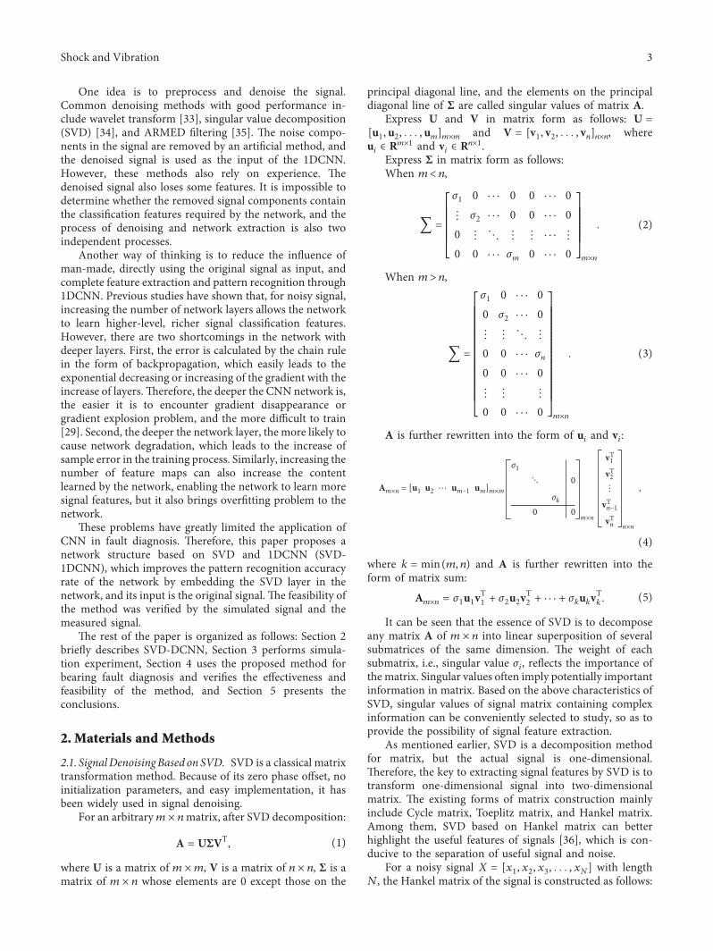
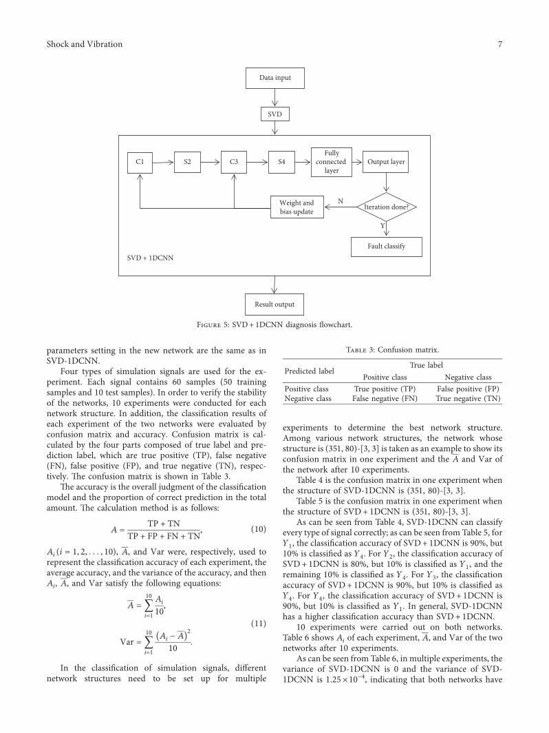
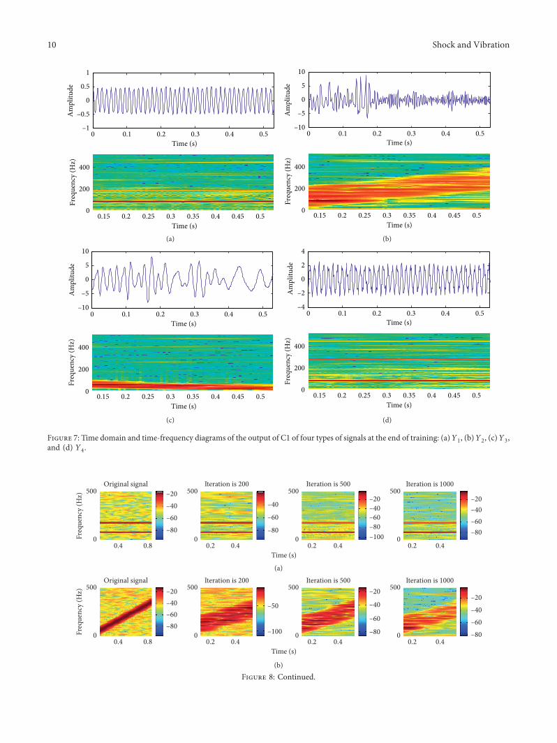
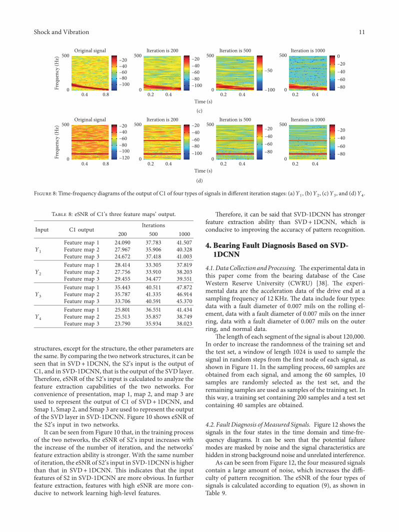
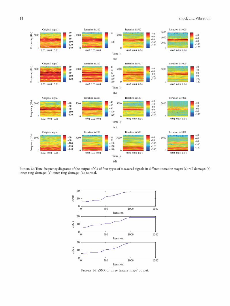
002 004 0060
5000
Time (s)
Freq
uenc
y (H
z)
ndash140ndash120ndash100ndash80ndash60ndash40
002 003 0040
5000
Iteration is 200
ndash100
ndash50Original signal
002 003 0040
5000
Iteration is 500
ndash120ndash100ndash80ndash60ndash40
002 003 0040
2000
4000
6000Iteration is 1000
ndash120ndash100ndash80ndash60ndash40
(a)
Time (s)
Freq
uenc
y (H
z)
002 004 0060
5000
ndash120ndash100ndash80ndash60ndash40
002 003 0040
5000
ndash140ndash120ndash100ndash80ndash60ndash40
002 003 0040
5000
ndash120ndash100ndash80ndash60ndash40
002 003 0040
5000
ndash120ndash100ndash80ndash60ndash40ndash20
Iteration is 200Original signal Iteration is 500 Iteration is 1000
(b)
Time (s)
Freq
uenc
y (H
z)
002 004 0060
5000
ndash120ndash100ndash80ndash60ndash40
002 003 0040
5000
ndash120ndash100ndash80ndash60ndash40
002 003 0040
5000
ndash120ndash100ndash80ndash60ndash40ndash20
002 003 0040
5000
ndash100ndash80ndash60ndash40ndash20
Iteration is 200Original signal Iteration is 500 Iteration is 1000
(c)
Time (s)
Freq
uenc
y (H
z)
002 004 0060
5000
ndash140ndash120ndash100ndash80ndash60
002 003 0040
5000
ndash140ndash120ndash100ndash80ndash60
002 003 0040
5000
ndash140ndash120ndash100ndash80ndash60
002 003 0040
5000
ndash120ndash100ndash80ndash60ndash40
Iteration is 200Original signal Iteration is 500 Iteration is 1000
(d)
Figure 13 Time-frequency diagrams of the output of C1 of four types of measured signals in different iteration stages (a) roll damage (b)inner ring damage (c) outer ring damage (d) normal
0
10
20
0
10
20
0 500 1000 15000
10
20
Iteration
0 500 1000 1500Iteration
0 500 1000 1500Iteration
eSN
ReS
NR
eSN
R
Figure 14 eSNR of three feature mapsrsquo output
14 Shock and Vibration
the measured signals the convolution kernel also selectivelyfilters out the noise in the original signals and as the numberof iteration increases the denoising effect is more significant
In addition eSNR of the S2rsquo input of SVD+ 1DCNN andSVD-1DCNN is calculated as shown in Figure 15
As can be seen from Figure 15 for the measured signalssimilarly in the training of the two networks eSNR of theS2rsquos input increases as the number of iteration increases Atthe same number of iteration eSNR of the S2rsquos input inSVD-1DCNN is higher than that in SVD+ 1DCNN-rough the experimental analysis of the measured signals
it can be said that SVD-1DCNN has stronger feature ex-traction ability than SVD+ 1DCNN-e confusion matricesof SVD-1DCNN and SVD+1DCNN in this classificationprocess are shown in Tables 10 and 11
As can be seen from Table 10 SVD-1DCNN can cor-rectly classify each type of measured signals According toTable 11 for roll damage signal the classification accuracy ofSVD+ 1DCNN is 90 but 10 is classified as normal signalFor inner ring damage signal the classification accuracy ofSVD+ 1DCNN is 90 but 10 is classified as outer ringdamage signal For outer ring damage signal the
0 500 1000 15000
50
Iteration
eSN
ReS
NR
eSN
R
0
50
0
50
Smap 3Map 3
0 500 1000 1500Iteration
Smap 2Map 2
0 500 1000 1500Iteration
Smap 1Map 1
Figure 15 eSNR of the S2rsquos input of the two networks
Table 10 Confusion matrix of SVD-1DCNN for classification results of measured signals
Predicted labelTrue label ()
Roll damage Inner ring damage Outer ring damage NormalRoll damage 100 0 0 0Inner ring damage 0 100 0 0Outer ring damage 0 0 100 0Normal 0 0 0 100
Table 11 Confusion matrix of SVD+ 1DCNN for classification results of measured signals
Predicted labelTrue label ()
Roll damage Inner ring damage Outer ring damage NormalRoll damage 90 0 0 10Inner ring damage 0 90 10 0Outer ring damage 0 10 90 0Normal 10 0 0 90
Shock and Vibration 15
classification accuracy of SVD+ 1DCNN is 90 but 10 isclassified as inner ring damage signal For normal signal theclassification accuracy of SVD+ 1DCNN is 90 but 10 isclassified as roll damage signal For measured signals SVD-1DCNN had a higher classification accuracy thanSVD+ 1DCNN
10 experiments were carried out on both networksTable 12 shows Ai of each experiment A and Var of the twonetworks after 10 experiments
As can be seen from Table 12 in the classification ofmeasured signals both networks have excellent stability andthe experimental results of SVD-1DCNN are better thanthose of SVD+ 1DCNN
5 Conclusions
-is paper proposes a fault diagnosis method based on SVDand 1DCNN which takes the original signals as input andavoids the loss of feature information -e feasibility of themethod is verified by experiments of simulated signals andmeasured signals In addition the role of convolutionkernels in feature extraction is also analyzed -e mainconclusions can be summarized as follows
A novel network structure SVD-1DCNN is con-structed by embedding an SVD layer after the first con-volution layer of 1DCNN In the novel network the SVDlayer denoises and reconstructs the output of the firstconvolution layer (primary classification feature) toachieve joint optimization of feature extraction anddenoising and reconstruction and the output of the SVDlayer is used as input to the next pooling layer Experimentsshow that the method has higher pattern recognition ac-curacy which shows SVD-1DCNN is more conducive tothe accurate diagnosis of bearing faults
By analyzing the output of the first convolution layer it isfound that the convolution kernels in the network extractdifferent frequency components for different signals andfilter out other frequency components In the trainingprocess the convolution kernel plays the role of extractingfeatures and denoising and as the number of networktraining increases the denoising effect of the convolutionkernel is better
Data Availability
-e data used to support the findings of this study areavailable in [39]
Conflicts of Interest
-e authors declare that they have no conflicts of interest
Acknowledgments
-is research was funded by the National Natural ScienceFoundation of China (grant number 51705531)
References
[1] R Liu G Meng B Yang C Sun and X Chen ldquoDislocatedtime series convolutional neural architecture an intelligentfault diagnosis approach for electric machinerdquo IEEE Trans-actions on Industrial Informatics vol 13 no 3 pp 1310ndash13202017
[2] W Sun B Yao N Zeng et al ldquoAn intelligent gear faultdiagnosis methodology using a complex wavelet enhancedconvolutional neural networkrdquo Materials vol 10 no 7pp 790ndash807 2017
[3] G Jiang H He J Yan and X Ping ldquoMultiscale convolutionalneural networks for fault diagnosis of wind turbine gearboxrdquoIEEE Transactions on Industrial Electronics vol 66 no 4pp 3196ndash3207 2018
[4] N R Safin V A Prakht V A Dmitrievskii andA A Dmitrievskii ldquoStator current fault diagnosis of induc-tion motor bearings based on the fast Fourier transformrdquoRussian Electrical Engineering vol 87 no 12 pp 661ndash6652016
[5] J Burrielvalencia R Puchepanadero J Martinezroman andM Pinedasanchez ldquoFault diagnosis of induction machines ina transient regime using current sensors with an optimizedslepian windowrdquo Sensors vol 18 no 2 pp 146ndash169 2018
[6] M Kang J Kim and J-M Kim ldquoAn FPGA-based multicoresystem for real-time bearing fault diagnosis using ultra-sampling rate AE signalsrdquo IEEE Transactions on IndustrialElectronics vol 62 no 4 pp 2319ndash2329 2015
[7] F K Choy W Jia and R Wu ldquoIdentification of bearing andgear tooth damage in a transmission systemrdquo TribologyTransactions vol 52 no 3 pp 303ndash309 2009
[8] Z Zhi Y S Zhu Y Y Zhang Y Xing and H H Shi ldquoFaultdiagnosis of rolling bearings based on EMD Interval--reshold denoising and maximum likelihood estimationrdquoJournal of Vibration and Shock vol 32 no 9 pp 155ndash1592013
[9] K H Hui L M Hee M S Leong and A M AbdelrhmanldquoTime-frequency signal analysis in machinery fault diagnosisreviewrdquo Advanced Materials Research vol 845 pp 41ndash452014
[10] S P Mogal and D I Lalwani ldquoA brief review on fault di-agnosis of rotating machineriesrdquo Applied Mechanics andMaterials vol 541-542 no 2 pp 635ndash640 2014
[11] Q Wang Y B Liu X He S Y Liu and J H Liu ldquoFaultdiagnosis of bearing based on KPCA and KNN methodrdquoAdvanced Materials Research vol 986-987 pp 1491ndash14962014
[12] S-W Fei ldquoFault diagnosis of bearing based on wavelet packettransform-phase space reconstruction-singular value
Table 12 Ai A and Var of SVD-1DCNN and SVD+ 1DCNN
SVD-1DCNN SVD+1DCNN1 100 9252 100 8753 100 904 100 905 100 906 100 907 100 908 100 909 100 9010 100 90A 100 90Var 0 125 times 10minus 4
16 Shock and Vibration
decomposition and SVM classifierrdquo Arabian Journal forScience and Engineering vol 42 no 5 pp 1967ndash1975 2017
[13] A K Mahamad and T Hiyama ldquoDevelopment of ANN fordiagnosing induction motor bearing failurerdquo IEEJ Transac-tions on Industry Applications vol 130 no 7 pp 838ndash8462010
[14] X Dai and Z Gao ldquoFrom model signal to knowledge a data-driven perspective of fault detection and diagnosisrdquo IEEETransactions on Industrial Informatics vol 9 no 4pp 2226ndash2238 2013
[15] Z W Gao C Cecati and S Ding ldquoA survey of fault diagnosisand fault-tolerant techniquesmdashpart II fault diagnosis withknowledge-based and hybridactive approachesrdquo IEEETransactions on Industrial Electronics vol 62 no 6pp 3768ndash3774 2015
[16] K Noda Y Yamaguchi K Nakadai H G Okuno andT Ogata ldquoAudio-visual speech recognition using deeplearningrdquo Applied Intelligence vol 42 no 4 pp 722ndash7372015
[17] S Nagpal M Singh R Singh and M Vatsa ldquoRegularizeddeep learning for face recognition with weight variationsrdquoIEEE Access vol 3 pp 3010ndash3018 2015
[18] S Nie M Zheng and Q Ji ldquo-e deep regression bayesiannetwork and its applications probabilistic deep learning forcomputer visionrdquo IEEE Signal Processing Magazine vol 35no 1 pp 101ndash111 2018
[19] T-H Chan K Jia S Gao J Lu Z Zeng and YMa ldquoPCANeta simple deep learning baseline for image classificationrdquo IEEETransactions on Image Processing vol 24 no 12 pp 5017ndash5032 2015
[20] W Long X Li G Liang and Y Zhang ldquoA new convolutionalneural network based data-driven fault diagnosis methodrdquoIEEE Transactions on Industrial Electronics vol 65 no 7pp 5990ndash5998 2018
[21] E Ozkural ldquo-e Foundations of Deep Learning with a Pathtowards General Intelligencerdquo in Proceedings of the Inter-national Conference on Artificial General Intelligencepp 162ndash173 Prague Czech Republic August 2018
[22] H Ren J-F Qu Y Chai Q Tang and X Ye ldquoDeep learningfor fault diagnosis the state of the art and challengerdquo Controland Decision vol 32 no 8 pp 1345ndash1358 2017
[23] B P Duong and J M Kim ldquoNon-mutually exclusive deepneural network classifier for combined modes of bearing faultdiagnosisrdquo Sensors vol 18 no 4 pp 1129ndash1143 2018
[24] H Shao H Jiang H Zhang W Duan T Liang and S WuldquoRolling bearing fault feature learning using improved con-volutional deep belief network with compressed sensingrdquoMechanical Systems and Signal Processing vol 100 pp 743ndash765 2018
[25] Z Chen and W Li ldquoMultisensor feature fusion for bearingfault diagnosis using sparse autoencoder and deep beliefnetworkrdquo IEEE Transactions on Instrumentation and Mea-surement vol 66 no 7 pp 1693ndash1702 2017
[26] W Lu X Wang C Yang and T Zhang ldquoA novel featureextraction method using deep neural network for rollingbearing fault diagnosisrdquo in Proceedings of the 27th ChineseControl and Decision Conference (2015 CCDC) QingdaoChina May 2015
[27] H Shao H Jiang X Zhang and M Niu ldquoRolling bearingfault diagnosis using an optimization deep belief networkrdquoMeasurement Science and Technology vol 26 no 11p 115002 2015
[28] Y Lecun Y Bengio and G Hinton ldquoDeep learningrdquo Naturevol 521 no 7553 pp 436ndash444 2015
[29] D Peng Z Liu H Wang Y Qin and L Jia ldquoA novel deeperone-dimensional CNN with residual learning for fault diag-nosis of wheelset bearings in high-speed trainsrdquo IEEE Accessvol 7 pp 10278ndash10293 2018
[30] X Min L Teng X Lin L Liu and C W D Silva ldquoFaultdiagnosis for rotating machinery using multiple sensors andconvolutional neural networksrdquo IEEEASME Transactions onMechatronics vol 23 no 1 pp 101ndash110 2017
[31] S Li G Liu X Tang J Lu and J Hu ldquoAn ensemble deepconvolutional neural network model with improved D-Sevidence fusion for bearing fault diagnosisrdquo Sensors vol 17no 8 pp 1729ndash1747 2017
[32] S Guo T Yang W Gao and C Zhang ldquoA novel fault di-agnosis method for rotating machinery based on a con-volutional neural networkrdquo Sensors vol 18 no 5pp 1429ndash1444 2018
[33] B Vidakovic and C B Lozoya ldquoOn time-dependent waveletdenoisingrdquo IEEE Transactions on Signal Processing vol 46no 9 pp 2549ndash2554 1998
[34] X Zhao and B Ye ldquoSelection of effective singular values usingdifference spectrum and its application to fault diagnosis ofheadstockrdquoMechanical Systems and Signal Processing vol 25no 5 pp 1617ndash1631 2011
[35] N Sawalhi R B Randall and H Endo ldquo-e enhancement offault detection and diagnosis in rolling element bearings usingminimum entropy deconvolution combined with spectralkurtosisrdquo Mechanical Systems and Signal Processing vol 21no 6 pp 2616ndash2633 2007
[36] H Jiang J Chen G Dong T Liu and G Chen ldquoStudy onHankel matrix-based SVD and its application in rolling el-ement bearing fault diagnosisrdquoMechanical Systems and SignalProcessing vol 52-53 no 1 pp 338ndash359 2015
[37] Z H Meng and C Wang ldquoApplication of rolling bearingcompound fault diagnosis based on combined SVDrdquoManufacturing Automation vol 35 no 21 pp 90ndash92 2013
[38] X Z Zhao B Y Ye and T J Tong ldquoDifference spectrumtheory of singular value and its application to the fault di-agnosis of headstock of latherdquo Journal of Mechanical Engi-neering vol 46 no 1 pp 100ndash108 2010
[39] CWRU Case Western Reserve University Bearing DateCenter Website CWRU Cleveland OH USA 2008httpcsegroupscaseedubearingdatecenterhome
Shock and Vibration 17
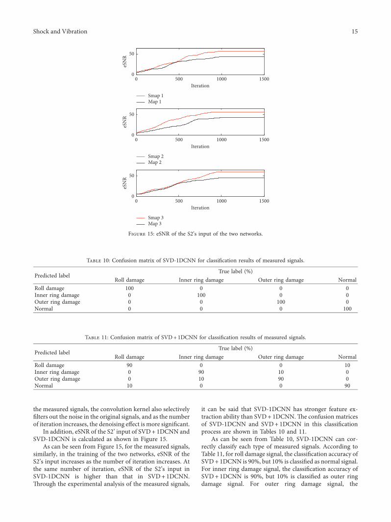
Related Documents