A Novel Analytical Method for Evolutionary Graph Theory Problems

A Novel Analytical Method for Evolutionary Graph

Theory Problems

Paulo Shakarian

Network Science Center and Dept. of Electrical Engineering and Computer Science,

United States Military Academy, West Point, NY 10996

Patrick Roos

Dept. of Computer Science, University of Maryland, College Park, MD 20740

Geoffrey Moores

Network Science Center and Dept. of Electrical Engineering and Computer Science,United States Military Academy, West Point, NY 10996

Abstract

Evolutionary graph theory studies the evolutionary dynamics of populationsstructured on graphs. A central problem is determining the probability thata small number of mutants overtake a population. Currently, Monte Carlosimulations are used for estimating such fixation probabilities on general di-rected graphs, since no good analytical methods exist. In this paper, weintroduce a novel deterministic framework for computing fixation probabil-ities for strongly connected, directed, weighted evolutionary graphs underneutral drift. We show how this framework can also be used to calculatethe expected number of mutants at a given time step (even if we relax theassumption that the graph is strongly connected), how it can extend to otherrelated models (e.g. voter model), how our framework can provide non-trivialbounds for fixation probability in the case of an advantageous mutant, andhow it can be used to find a non-trivial lower bound on the mean time tofixation. We provide various experimental results determining fixation prob-abilities and expected number of mutants on different graphs. Among these,we show that our method consistently outperforms Monte Carlo simulationsin speed by several orders of magnitude. Finally we show how our approachcan provide insight into synaptic competition in neurology.

Preprint submitted to BioSystems January 14, 2013

arX

iv:1

301.

2533

v1 [

cs.G

T]

11

Jan

2013

Keywords: evolutionary dynamics, Moran process, complex networks

1. Introduction

Evolutionary graph theory (EGT), introduced by [14], studies the prob-lems related to population dynamics when the underlying structure of thepopulation is represented as a directed, weighted graph. This model hasbeen applied to problems in evolutionary biology [28], physics [25], gametheory [20], neurology [26], and distributes systems [13]. A central problemin this research area is computing the fixation probability - the probabilitythat a certain subset of mutants overtakes the population. Although goodanalytical approximations are available for the undirected/unweighted case[1, 6], these break down for directed, weighted graphs as shown by [16]. Asa result, most work dealing with evolutionary graphs rely on Monte Carlosimulations to approximate the fixation probability [22, 7, 4]. In this paperwe develop a novel deterministic framework to compute fixation probabilityin the case of neutral drift (when mutants and residents have equal fitness)in directed, weighted evolutionary graphs based on the convergence of “ver-tex probabilities” to the fixation probability as time approaches infinity. Wethen show how this framework can be used to calculate the expected numberof mutants at a given time, how the framework can be modified to do thesame for related models, how it can provide non-trivial bounds for fixationprobability in the case of an advantageous mutant, and how it can providea non-trivial lower bound on the mean time to fixation. We also providevarious experiments that show how our method can outperform Monte Carlosimulations by several orders of magnitude. Additionally, we show that theresults of this paper can provide direct insight into the problem of synapticcompetition in neurology.

Our method also fills a few holes in the literature. First, it allows fordeterministic computation of fixation probability when there is an initialset of mutants – not just a singleton (the majority of current research onevolutionary graph theory only considers singletons). Second, it allows usto study how the mutant population changes as a function of time. Third,we show (by way of rigorous proof) that fixation probability, under the caseof neutral drift is a lower bound for the case of the advantageous mutant -confirming simulation observations by [15]. Fourth, we show (also by way ofrigorous proof) that fixation probability under neutral drift is additive (even

2

for weighted, directed graphs), which extends the work of [6] that provedthis for undirected/unweighted graphs. Fifth, we provide a non-trivial lowerbound for the computation of mean time to fixation in the general case -which has only previously been explored for well-mixed populations [2] andspecial cases of graphs [5].

This paper is organized as follows. In Section 2 we review the originalmodel of Lieberman et al., introduce the idea of “vertex probabilities” andshow how they can be used to find the fixation probability. We then show howthis can be used to determine the expected number of mutants at a giventime in Section 3. This is followed by a discussion of how the frameworkcan be extended to other update rules in Section 4 and then for boundingfixation probability in the case of an advantageous mutant in Section 5.We then discuss how our approach can be adopted to bound mean time tofixation in Section 6. We use the results of the previous sections to createan algorithm for computing fixation probability and introduce a heuristictechnique to significantly decrease the run-time. The algorithm and severalexperimental evaluations are described in Section 7. In Section 8, we showhow our framework can be applied to neurology to gain insights into synapticcompetition. Finally, we discuss related work in Section 9 and conclude.

2. Directly Calculating Fixation Probability

The classic evolutionary model known as the Moran Process is a stochas-tic process used to describe evolution in a well-mixed population [18]. Allthe individuals in the population are either mutants or residents. The aim ofsuch work was to determine if a set of mutants could take over a populationof residents (achieving “fixation”). In [14], evolutionary graph theory (EGT)is introduced, which generalizes the model of the Moran Process by speci-fying relationships between the N individuals of the population in the formof a directed, weighted graph. Here, the graph will be specified in the usualway as G = (V,E) where V is a set of nodes (individuals) and E ⊆ V × V .In most literature on evolutionary graph theory, the evolutionary graph isassumed to be strongly connected. We make the same assumption and statewhen it can be relaxed.

For any node i, the numbers k(i)in , k

(i)out are the in- and out- degrees respec-

tively. We will use the symbol N to denote the sized of V . Additionally,we will specify weights on the edges in set E using a square matrix denotedW = [wij] whose side is of size N . Intuitively, wij is the probability that

3

member of the population j is replaced by i given that member i is selected.We require

∑j wij = 1 and that (i, j) ∈ E iff wij > 0. If for all i, j, we have

wij = 1/k(i)out, then the graph is said to be “unweighted.” If for all (i, j) ∈ E,

we have (j, i) ∈ E the graph is said to be “undirected.” Though our resultsprimarily focus on the general case, we will often refer to the special caseof undirected/unweighted graphs as this special case is quite common in theliterature [1, 6].

In this paper we will often consider the outcome of the evolutionary pro-cess when there is a set of initial mutants as opposed to a singleton. Hence,we say some set (often denoted C) is a configuration if that set specifies theset of mutants in the population (all other members in the population thenare residents). We assume all members in the population are either mutantsor residents and have a fitness specified by a parameter r > 0. Mutantshave a fitness r and residents have a fitness of 1. At each time step, someindividual i ∈ V is selected for “birth” with a probability proportional to itsfitness. Then, an outgoing neighbor j of i is selected with probability wijand replaced by a clone of i. Note if r = 1, we say we are in the special caseof neutral drift.

We will use the notation PV ′,t to refer to the probability of being inconfiguration V ′ after t timesteps and PV ′,t|C to be the probability of being inconfiguration V ′ at time t conditioned upon initial configuration C. Perhapsthe most widely studied problem in evolutionary graph theory is to determinethe fixation probability. Given set of mutants C at time 0, the fixationprobabilty is defined as follows.

FC = limt→∞PV,t|C (1)

This is the probability that an initial set C of mutants takes over the en-tire population as time approaches infinity. Similarly, we will use the termthe extinction probability, FC , to be limt→∞P∅,t|C . If the graph if stronglyconnected, then we have FC + FC = 1. Hence, for a strongly connectedgraph, a mutant either fixates or becomes extinct. Typically, this problemis studied using Monte Carlo simulation. This work uses the idea of a ver-tex probabilities to create an alternative to such an approach. The vertexprobability is the probability that a certain vertex is a mutant at a certaintime given an initial configuration. For vertex i at time t, we denote this asPi,t|C . Often, for ease of notation, we shall assume that the probabilities areconditioned on some initial configuration and drop the condition, writing Pi,t

4

instead of Pi,t|C . We note that Pi,t can be expressed in terms of probabilitiesof configurations as follows.

Pi,t =∑V ′∈2V

s.t. i∈V ′

PV ′,t (2)

Viewing the probability that a specific vertex is a mutant at a given timehas not, to our knowledge, been studied before with respect to evolutionarygraph theory (or in related processes such as the voter model). The keyinsight of this paper is that studying these probabilities sheds new light onthe problem of calculating fixation probabilities in addition to providing otherinsights into EGT. For example, it is easy to show the following relationship.

Proposition 1. Let V ′ be a subset of V and t be an arbitrary time point.Iff for all i ∈ V ′, Pi,t = 1 and for all i /∈ V ′, Pi,t = 0, then PV ′,t = 1 and forall V ′′ ∈ 2V s.t. V ′′ 6≡ V ′, PV ′′,t = 0.

It is easy to verify that FC > 0 iff ∀i ∈ V , limt→∞Pi,t > 0. Hence, in thispaper, we shall generally assume that limt→∞Pi,t > 0 holds for all vertices iand specifically state when it does not. As an aside, for a given graph, thisassumption can be easily checked: simply ensure for j ∈ V − C that existssome i ∈ C s.t. there is a directed path from i to j.

Now that we have introduced the model and the idea of vertex proba-bilities we will show how to leverage this information to compute fixationprobability. It is easy to show that as time approaches infinity, the vertexprobabilities for all vertices converge to the fixation probability when thegraph if strongly connected.

Theorem 1. ∀i, limt→∞ Pi,t|C = FC

Now let us consider how to calculate Pi,t for some i and t. For t = 0,where we know that we are in the state where only vertices in a given set aremutants, we need only appeal to Proposition 1 - which tells us that we assigna probability of 1 to all elements in that set and 0 otherwise. For subsequenttimesteps, we have developed Theorem 2 shown next (the proof of which isincluded in the supplement).

5

Theorem 2.

Pi,t = Pi,t−1 +∑

(j,i)∈E

wji(Pj,t−1 · S(j,t)|(j,t−1) − Pi,t−1 · S(j,t)|(i,t−1)

)(S(j,t)|(i,t−1) is the probability that j is picked for reporduction at time t giventhat i was a mutant at time t− 1.)

We believe that a concise, tractable analytical solution for S(j,t)|(i,t−1) is un-likely. However, for neutral drift (r = 1), these conditional probabilities aretrivial - specifically, we have for all i, j, t, S(j,t)|(i,t−1) = 1/N as this probabilityof selection is independent of the current set of mutants or residents in thegraph. Hence, in the case of neutral drift, we have the following:

Pi,t = Pi,t−1 +∑

(j,i)∈E

wjiN· (Pj,t−1 − Pi,t−1) (3)

Studying evolutionary graph theory under neutral drift was a central themein several papers on EGT in the past few years [6, 15] as it provides anintuition on the effects of network topology on mutant spread. In Section 5we examine the case of the advantageous mutant (r > 1). Neutral drift allowsus to strengthen the statement of Equation 1 to a necessary and sufficientcondition - showing that when the probabilities of all nodes are equal, thenwe can determine the fixation probability.

Theorem 3. Assuming neutral drift (r = 1), given initial configuration Cwith fixation probability FC, if at time t the quantities Pi,t|C are equal (for alli ∈ V ), then they also equal FC.

Therefore, under neutral drift, we can determine fixation probability whenEquation 3 causes all Pi,t’s to be equal. We can also use Equation 3 to findbounds on the fixation probability for some time t by the following resultthat holds for any time t under neutral drift.

miniPi,t ≤ FC ≤ max

iPi,t (4)

Under neutral drift, we can show that fixation probability is additive fordisjoint sets. Broom et al. proved a similar result the a special case of undi-rected/unweighted evolutionary graphs [6]. However, our proof (contained in

6

the supplement) differs from theirs in that we leverage Equation 3. Further,unlike the result of Broom et al., our result applies to the more general caseof weighted, directed graphs.

Theorem 4. When r = 1 for disjoint sets C,D ⊆ V , FC + FD = FC∪D.

3. Calculating the Expected Number of Mutants

In addition to allowing for the calculation of fixation probability, ourframework can also be used to observe how the expected number of mutantschanges over time. We will use the notation Ex

(t)C to denote the expected

number of mutants at time t given initial set C. Formally, this is definedbelow.

Ex(t)C =

∑i∈V

Pi,t (5)

Unlike fixation probability, which only considers the probability that mu-tants overtake a population, Ex

(t)C provides a probabilistic average of the

number of mutants in the population under a finite time horizon. For exam-ple, is has been noted that graph structures which amplify fixation normallyalso increase time to absorption [8, 21]. Hence, finding the expected numberof mutants may be a more viable topic in some areas of research where timeis known to be limited. Following from Equation 3 where we showed how tocompute Pi,t for each node at a given time, we have the following relationshipconcerning the expected number of mutants at a given time under neutraldrift.

Ex(t)C = Ex

(t−1)C +

Ex(t−1)C

N− 1

N

∑i∈V

∑(j,i)∈E

wji · Pi,t−1 (6)

Based on Equation 6, we notice that for r = 1, at each time-step, thenumber of expected mutants increases by at most the average fixation prob-ability and decreases by a quantity related to the average “temperature.”The temperature of vertex i (denoted Ti) is defined for a given node is thesum of the incoming edge weights [14]: Ti =

∑j wji. Intuitively, nodes with

a higher temperature change more often between being a mutant and being a

7

resident than those with lower temperature. Re-writing Equation 6 in termsof temperature we have the following:

Ex(t)C = Ex

(t−1)C +

Ex(t−1)C

N− 1

N

∑i∈V

Ti · Pi,t−1 (7)

Hence, if the preponderance of high temperature nodes are likely to bemutants, then most likely the average number of mutants will decrease at thenext time step. We also note that Theorem 2, Equation 3, and Equation 6do not depend on the assumption that the underlying graph is strongly con-nected. Therefore, as such is the case, we can study the relationship of timevs. expected number of mutants for any evolutionary graph (under neutraldrift). This could be of particular interest to non-strongly connected evolu-tionary graphs that may have trivial fixation probabilities (i.e. 1 or 0) butmay have varying levels of mutants before achieving an absorbing state.

4. Applying the Framework to Other Update Rules

The results of the last two sections not only apply to the original model of[14], but several other related models in the literature. Viewing an evolution-ary graph problem as a stochastic process, where the states represent differentmutant-resident configurations, it is apparent that the original model spec-ifies the transition probabilities. However, there are other ways to specifythe transition probabilities known as update rules. Several works addressdifferent update rules [1, 25, 15]. Overall, we have identified three majorfamilies of update rules - birth-death (a.k.a. the invasion process) where thenode to reproduce is chosen first, death-birth (a.k.a. the voter model) wherethe node to die is chosen first, and link dynamics, where an edge is chosen.We summarize these in Table 1.

We have already shown how our methods can deal with the original modelof Lieberman et al., often referred to as the Birth-Death (BD) process. Inthis section, we apply our methods to the neutral-drift (non-biased) cases ofdeath-birth and link-dynamics. In these models, the weights of the edges istypically not considered. Hence, in order to align this work with the majorityof literature on those models, we will express vertex probabilities in terms ofnode in-degree (k

(i)in ) and the set of directed edges (E). We note that these

results can be easily extended to a more general case with an edge-weightmatrix as we used for the original model of EGT.

8

Table 1: Different families of update rules.

Update Rule Intuition

Birth-Death (BD) (1) Node i selected(a.k.a. Invasion Process (IP)) (2) neighbor of i, node j selected

(3) Offspring of i replaces jDeath-Birth (DB) (1) Node i selected(a.k.a. Voter Model (VM)) (2) neighbor of i, node j selected

(3) Offspring of j replaces iLink Dynamics (LD) (1) Edge (i, j) selected

(2) The offspring of one node in theedge replaces the other node

4.1. Death-Birth Updating

Under the death birth model (DB), at each time step, a vertex i is selectedfor death. With a death-bias (DB-D), it is selected proportional to the inverseof its fitness, with a birth-bias (DB-B) it is selected with a probability 1/N ,which is also the probability under neutral drift. Then, an incoming neighbor(j) is selected either proportional to the fitness of all incoming neighbors(birth-bias), or with a uniform probability (in the case death-bias or neutraldrift). The selected neighbor then replaces i. Here, we compute Pi,t underthis dynamic with r = 1.

Pi,t = (1−N−1)Pi,t−1 + (Nk(i)in )−1

∑(j,i)∈E

Pj,t−1 (8)

We note that the proof of convergence still holds for death-birth - thatis for some time t, ∀i, the value Pi,t is the same, then Pi,t = FC . Further,Theorem 4 holds for DB under neutral drift as well, specifically, for disjointsets C,D ⊆ V , FC + PD = PC∪D.

4.2. Link-Dynamics

With link dynamics (LD), at each time step an edge (i, j) is selectedeither proportional to the fitness of i or the inverse of the fitness of j. Ithas previously been shown that LD under birth bias is an equivalent process

9

to LD with a death bias [15]. Under neutral drift, the probability of edgeselection is 1/|E| (where |E| is the cardinality of set E). Then, i replaces j.Now, we compute Pi,t under this dynamic with r = 1.

Pi,t = (1− k(i)in |E|−1)Pi,t−1 +

1

|E|∑

(j,i)∈E

Pj,t−1 (9)

Again, convergence and additivity of the fixation probability still holdunder link dynamics just as with BD and DB.

5. Bounding Fixation Probability for r > 1

So far we have shown how our method can be used to find fixation proba-bilities under the case of neutral drift. Here, we show how our framework canbe useful in the case of an advantageous mutant (when the value for r, therelative fitness, is greater than 1). First, we show that our method providesa lower bound. We then provide an upper bound on the fixation probabil-ity that can be used in conjunction with our framework when studying thecase of the advantageous mutant. We note that certain parts of these proofsare specific for diffent update rules, and we identify them using the abbre-viations from the last section (DB-D, DB-B, and LD). The update of theoriginal model of [14] is known as the “birth-death” model and abbreviatedBD. If the fitness bias is on a birth event, we denote it as BD-B and if thebias is on a death event we denote it as BD-D.

Naoki Masuda observes experimentally (through simulation) that the fix-ation probability computed with neutral drift appears to be a lower boundon the fixation probability for an advantageous mutant [15]. We were ableto prove this result analytically – the proof is included in the supplementarymaterials.

Theorem 5. For a given set C, let F(1)C be the fixation probability under

neutral drift and F(r)C be the fixation probability calculated using a mutant

fitness r > 1. Then, under BD-B, BD-D, DB-B, DB-D, or LD dynamics,F

(1)C ≤ F

(r)C .

This proof leads to the conjecture that r′ > r implies F(r′)C ≥ F

(r)C . How-

ever, we suspect that proving this monotonicity property will require a dif-ferent technique than used in Theorem 5. Next, to find an upper bound

10

that corresponds with the lower bound above, we use the proof technique in-troduced in [9], to obtain the following non-trivial upper bounds of fixationprobability for individual nodes in various update rules.

BD−B : F{i} ≤ r(r +∑j

wji)−1 (10)

BD−D : F{i} ≤

(∑j

wjir − rwji + wji

)−1

(11)

DB−B : F{i} ≤∑j

rwij(1− wij + rwij)−1 (12)

DB−D : F{i} ≤ r∑j

wij (13)

6. A Lower Bound for Mean Time to Fixation

Another important, although less-studied problem with respect to evolu-tionary graph theory is the mean time to fixation - the average time it takesfor a mutant to take over the population. Closely related to this problemare mean time to extinction (average time for the resident to take over) andmean time to absorption (average time for either mutant or resident to takeover). This has been previously studied under the original Moran processfor well mixed populations [2] as well as some special cases of graphs [5].However, to our knowledge, a general method to compute these quantities(without resorting to the use of simulation) have not been previously studied.Here we take a “first step” toward developing such a method by showing howthe techniques introduced in this paper can be used to compute a non-triviallower bound for mean time to fixation (and easily modified to bound meantime to extinction and absorption).

Let Ft|C be the probability of fixation at time t. Therefore, Ft|C − Ft−1|Cis the probability of entering fixation at time t. The symbol tC is the meantime. By the results of [2], we have the following:

Theorem 6.

tC =1

FC

∞∑t=1

t · (Ft|C − Ft−1|C)

11

Our key intuition is noticing that at each time step t, Ft|C ≤ mini Pi,t.From this, we use the accounting method to provide a rigorous proof for thefollowing theorem that provides a non-trivial lower-bound for the mean timeto fixation. This result can be easily modified for mean time to extinctionand absorption as well.

Theorem 7. 1FC

∑∞t=1 t·(Pmin,t−Pmin,t−1) ≤ 1

FC

∑∞t=1 t·(Ft|C−Ft−1|C) Where

Pmin,t = mini Pi,t.

7. Algorithm and Experimental Evaluation

We leverage the finding of the previous sections in Algorithm 1. As describedearlier, our method has found the exact fixation probability when all theprobabilities in

⋃i{Pi,t} (represented in the pseudo-code as the vector p) are

equal. We use Equation 4 to provide a convergence criteria based on valueε, which we can prove to be the tolerance for the fixation probability.

Proposition 2. Algorithm 1 returns the fixation probability FC within ±ε.

Our novel method for computing fixation probabilities on strongly con-nected directed graphs allows us to compute near-exact fixation probabilitieswithin a desired tolerance. The running time of the algorithm is highly de-pendent on how fast the vertex probabilities converge. In this section weexperimentally evaluate how the vertex probabilities in our algorithms con-verge. We also provide results from comparison experiments to support theclaim that Algorithm 1-ACC finds adequate fixation probabilities order ofmagnitudes faster than Monte Carlo simulations. We also show how the al-gorithm can be used to study the expected number of mutants as well asbound mean time to fixation.

7.1. Convergence of Vertex Probabilities

We ran our algorithm to compute fixation probabilities on randomlyweighted and strongly connected directed graphs in order to experimentallyevaluate the convergence of the vertex probabilities. We generated the graphsto be scale-free using the standard preferential attachment growth model [3]and randomly assigned an initial mutant node. We replaced all edges in thegraph given by the growth model with two directed edges and then randomlyassigned weights to all the edges.

12

Algorithm 1 - Our Novel Solution Method to Compute Fixation Probabil-itiesInput: Evolutionary Graph 〈N, V,W 〉, configuration C ⊆ V , natural numberR > 0, and real number ε ≥ 0.Output: Estimate of fixation probability of mutant.

1: pi is the ith position in vector p corresponding with vertex i ∈ V .2: Set pi = 1 if i ∈ C and pi = 0 otherwise. {As per Proposition 1}3: q← p {q will be p from the previous time step.}4: τ ← 15: while τ > ε do6: for i ∈ V {This loop carries out the calculation as per Equation 3}

do7: sum← 08: m← {j ∈ V |wji > 0}9: for j ∈ m do

10: sum = sum+ wji · (qj − qi)11: end for12: pi ← qi + 1/N · sum13: end for14: q← p15: τ ← (1/2)·(max p−min p) {Ensures error bound based on Equation 4}16: end while17: return (min p) + τ

13

0 20000 40000 60000 80000 100000t

0.00

0.02

0.04

0.06

0.08

0.10V

erte

x P

roba

bili

ty

MinP

MaxP

AvgPFinal

100 200 300 400 500

Graph Size (Number of Nodes)

104

105

106

Spe

edup

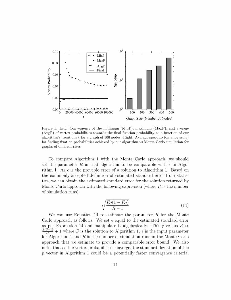
Figure 1: Left: Convergence of the minimum (MinP), maximum (MaxP), and average(AvgP) of vertex probabilities towards the final fixation probability as a function of ouralgorithm’s iterations t for a graph of 100 nodes. Right: Average speedup (on a log scale)for finding fixation probabilities achieved by our algorithm vs Monte Carlo simulation forgraphs of different sizes.

To compare Algorithm 1 with the Monte Carlo approach, we shouldset the parameter R in that algorithm to be comparable with ε in Algo-rithm 1. As ε is the provable error of a solution to Algorithm 1. Based onthe commonly-accepted definition of estimated standard error from statis-tics, we can obtain the estimated standard error for the solution returned byMonte Carlo approach with the following expression (where R is the numberof simulation runs). √

FC(1− FC)

R− 1(14)

We can use Equation 14 to estimate the parameter R for the MonteCarlo approach as follows. We set ε equal to the estimated standard erroras per Expression 14 and manipulate it algebraically. This gives us R ≈S(S−1)ε2

+ 1 where S is the solution to Algorithm 1, ε is the input parameterfor Algorithm 1 and R is the number of simulation runs in the Monte Carloapproach that we estimate to provide a comparable error bound. We alsonote, that as the vertex probabilities converge, the standard deviation of thep vector in Algorithm 1 could be a potentially faster convergence criteria.

14

0 20000 40000 60000 80000 100000t

0.01

0.02

0.03

0.04

0.05

0.06

0.07

0.08

0.09

0.10St

dev

of V

erte

x Pr

obab

ilitie

s

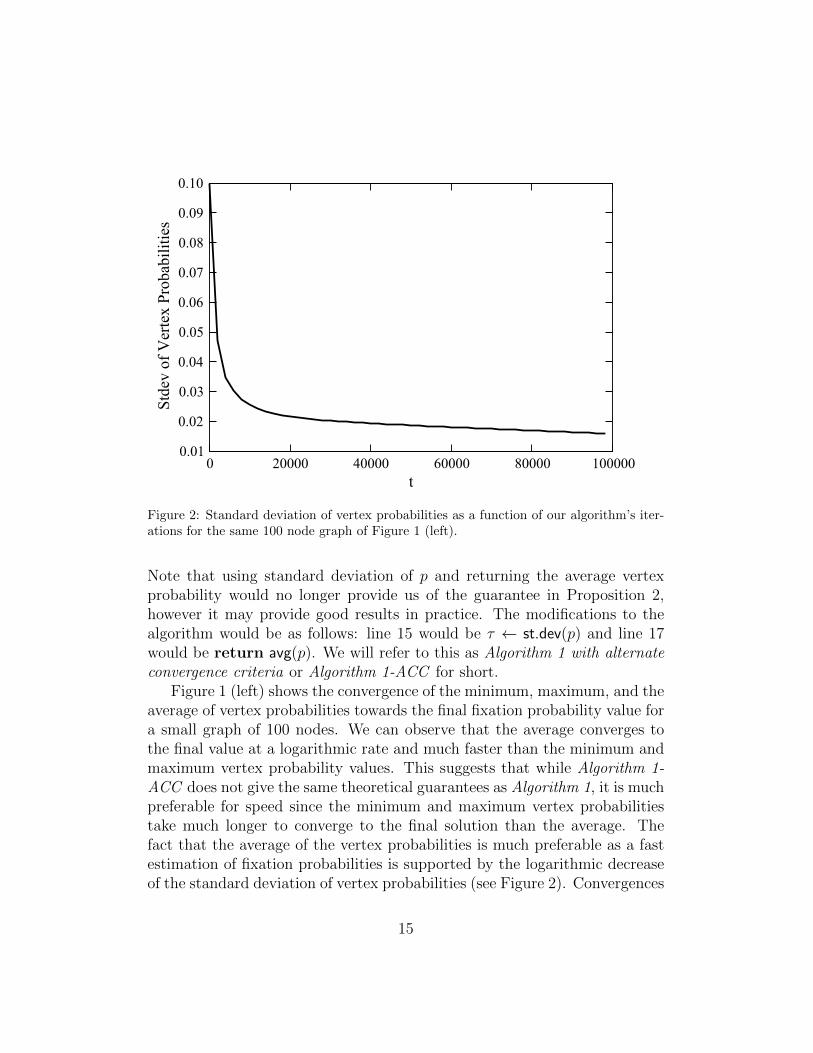
Figure 2: Standard deviation of vertex probabilities as a function of our algorithm’s iter-ations for the same 100 node graph of Figure 1 (left).

Note that using standard deviation of p and returning the average vertexprobability would no longer provide us of the guarantee in Proposition 2,however it may provide good results in practice. The modifications to thealgorithm would be as follows: line 15 would be τ ← st.dev(p) and line 17would be return avg(p). We will refer to this as Algorithm 1 with alternateconvergence criteria or Algorithm 1-ACC for short.

Figure 1 (left) shows the convergence of the minimum, maximum, and theaverage of vertex probabilities towards the final fixation probability value fora small graph of 100 nodes. We can observe that the average converges tothe final value at a logarithmic rate and much faster than the minimum andmaximum vertex probability values. This suggests that while Algorithm 1-ACC does not give the same theoretical guarantees as Algorithm 1, it is muchpreferable for speed since the minimum and maximum vertex probabilitiestake much longer to converge to the final solution than the average. Thefact that the average of the vertex probabilities is much preferable as a fastestimation of fixation probabilities is supported by the logarithmic decreaseof the standard deviation of vertex probabilities (see Figure 2). Convergences

15

for other and larger graphs are not shown here but are qualitatively similarto the relative convergences shown in the provided graphs.

7.2. Speed Comparison to Monte Carlo Simulation

In order to compare our method’s speed compared to the standard MonteCarlo simulation method, we must determine how many iterations our algo-rithm must be run to find a fixation probability estimate comparable to thatof the Monte Carlo approach. Thankfully, as we have seen, we can get astandard error on the fixation probability returned by the Monte Carlo ap-proach as per Equation 14. While we did not theoretically prove anythingabout how smoothly fixation probabilities from our methods approach thefinal solution, the convergences of the average and standard deviation asshown above strongly suggest that estimates from our method approach thefinal solution quite gracefully. In fact, in the following experiments, onceour method has arrived at a fixation probability estimate within the stan-dard error of simulations, the estimate never again fell outside the window ofstandard error (although the estimate did not always approach the final es-timate monotonically). This is in stark contrast to Monte Carlo simulations,from which estimations can vary greatly before the method has completedenough single runs to achieve a good probability estimate.

We generated a number of randomly weighted and strongly connecteddirected graphs of various sizes on which we compare our solution methodto Monte Carlo approximation of fixation probabilities. The graphs weregenerated as in our convergence experiments. For each graph of a differentsize, we generated a number of different initial mutant configurations. Wefound fixation probabilities both using Monte Carlo estimation with 2000simulation runs and our direct solution method, terminating when we havereached within the standard error of the Monte Carlo estimation. Since theaverage vertex probability proved to be such a good fast estimate of the truefixation probability, we used Algorithm 1-ACC.

Figure 1 (right) shows the speedup our solution provides over MonteCarlo simulation. Here speedup is defined as the ratio of the time it takesfor simulations to complete over the time it takes our algorithm to find afixation probability within the standard deviation. The often extremely lownumber of iterations needed by our algorithm to find fixation probabilitieswithin the standard error of simulations may prompt the concern that theprobabilities fall within this window so soon by mere chance. However, ourexperiments have shown that the fixation probability estimation found by

16

our algorithm at each iteration approaches the final fixation probability aftertermination smooothly at a logarithmic rate, asymptotically approaching thetrue fixation probability. While in this case the fixation probability estimateslightly crosses over the true fixation probability and then slowly approachesit again, none of the fixation probability estimates from our algorithm exitedthe window of standard error (from simulations) once they entered it.

We can observe from our experiments that computing fixation proba-bilities using Monte Carlo simulations showed to be a very time-expensiveprocess, highlighting the need for faster solution methods as the one we havepresented. Especially for larger graph sizes, the time complexity of our so-lution to achieve similar results to Monte Carlo simulation has shown to beorders of magnitude smaller than the standard method.

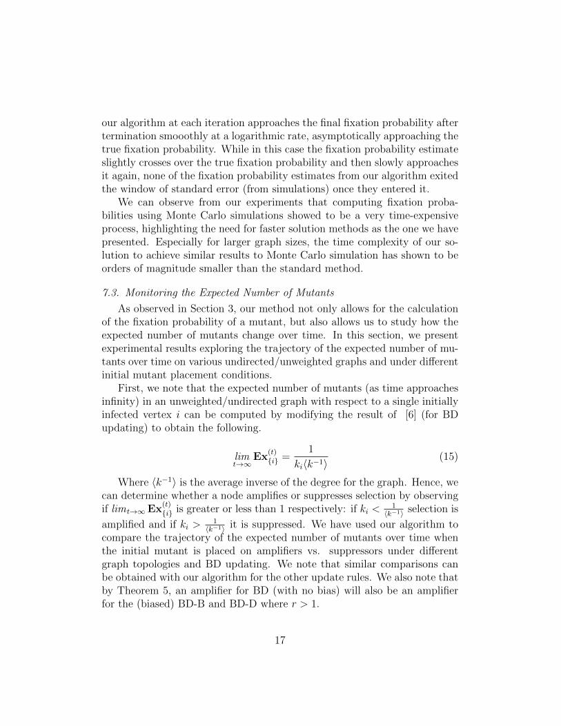
7.3. Monitoring the Expected Number of Mutants

As observed in Section 3, our method not only allows for the calculationof the fixation probability of a mutant, but also allows us to study how theexpected number of mutants change over time. In this section, we presentexperimental results exploring the trajectory of the expected number of mu-tants over time on various undirected/unweighted graphs and under differentinitial mutant placement conditions.

First, we note that the expected number of mutants (as time approachesinfinity) in an unweighted/undirected graph with respect to a single initiallyinfected vertex i can be computed by modifying the result of [6] (for BDupdating) to obtain the following.

limt→∞

Ex(t){i} =

1

ki〈k−1〉(15)

Where 〈k−1〉 is the average inverse of the degree for the graph. Hence, wecan determine whether a node amplifies or suppresses selection by observingif limt→∞Ex

(t){i} is greater or less than 1 respectively: if ki <

1〈k−1〉 selection is

amplified and if ki >1〈k−1〉 it is suppressed. We have used our algorithm to

compare the trajectory of the expected number of mutants over time whenthe initial mutant is placed on amplifiers vs. suppressors under differentgraph topologies and BD updating. We note that similar comparisons canbe obtained with our algorithm for the other update rules. We also note thatby Theorem 5, an amplifier for BD (with no bias) will also be an amplifierfor the (biased) BD-B and BD-D where r > 1.

17

0 100 200 300 400 500t

0.0

0.2

0.4

0.6

0.8

1.0

1.2

1.4

Expe

cted

Num

ber o

f Mut

ants

Mutant at Highest Degree

0 100 200 300 400 500t

0.0

0.2

0.4

0.6

0.8

1.0

1.2

1.4

Mutant at Lowest Degree

BA ERD NWS

Figure 3: Expected number of mutants over time starting with a single mutant placedon a graph for Barabasi-Albert preferential attachment (BAR), Erdos-Renyi (ERD), andNewmann-Watts-Strogatz small world (NWS) graphs. Lines are averages over 50 randomgraphs of each type. In the left graph, mutants are placed at the highest degree nodes,which are suppressors. In the right graph, mutants are placed at lowest degree nodes,which are amplifiers.

Figure 3 shows the trajectories of the expected number of mutants overtime on random [3] preferential attachment (BAR), [10] (ER), and [19] smallworld graphs (NWS), each for when the initial mutant is placed on a sup-pressor (highest degree node of graph) and amplifier (lowest degree node ofgraph). Graphs are all of equal size at 100 nodes. We note that the highestdegree nodes are especially strong suppressors on BAR graphs, less so forNWS graphs, and even less so for ER graphs. This makes sense when oneconsiders the degree distribution of the different graph topologies, which arescale-free or power-law (P (k) ∼ k−3) for BR, roughly Poisson-shaped forNWS, and relatively uniform for ER graphs. For lowest degree amplifiers,the expected number of mutants grows faster early on in Barabasi-Albertgraphs, but it plateaus earlier than and is eventually surpassed by the slowergrowing expected number of mutants in the Erdos-Renyi, and Newmann-Watts-Strogatz graphs. Such insights into the evolutionary process may be

18

0 20000 40000 60000 80000 100000t

0

10

20

30

40

50

60

70Ex

pect

ed N

umbe

r of M

utan

ts

dcon_mn< dcon_rn

dcon_mn≈ dcon_rn

dcon_mn> dcon_rn

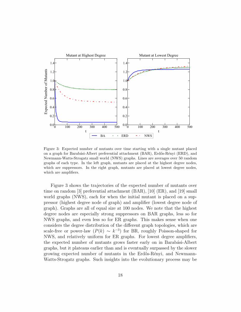
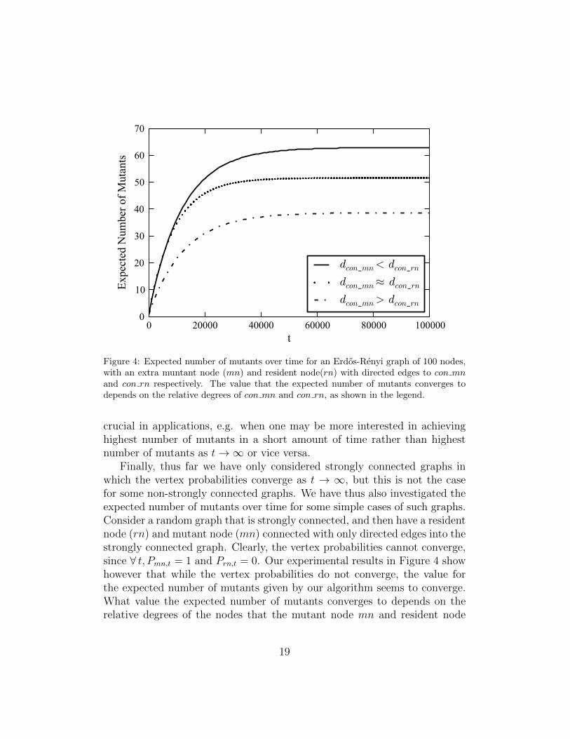
Figure 4: Expected number of mutants over time for an Erdos-Renyi graph of 100 nodes,with an extra muntant node (mn) and resident node(rn) with directed edges to con mnand con rn respectively. The value that the expected number of mutants converges todepends on the relative degrees of con mn and con rn, as shown in the legend.

crucial in applications, e.g. when one may be more interested in achievinghighest number of mutants in a short amount of time rather than highestnumber of mutants as t→∞ or vice versa.

Finally, thus far we have only considered strongly connected graphs inwhich the vertex probabilities converge as t → ∞, but this is not the casefor some non-strongly connected graphs. We have thus also investigated theexpected number of mutants over time for some simple cases of such graphs.Consider a random graph that is strongly connected, and then have a residentnode (rn) and mutant node (mn) connected with only directed edges into thestrongly connected graph. Clearly, the vertex probabilities cannot converge,since ∀ t, Pmn,t = 1 and Prn,t = 0. Our experimental results in Figure 4 showhowever that while the vertex probabilities do not converge, the value forthe expected number of mutants given by our algorithm seems to converge.What value the expected number of mutants converges to depends on therelative degrees of the nodes that the mutant node mn and resident node

19

rn connect to. We shall call these nodes con mn and con rn, respectively.If kcon mn ≈ kcon rn, the expected value of mutants converges at around 50%of the graph’s nodes. If kcon mn > kcon rn, the expected value of mutantsis less than 50% of the graph’s nodes, and conversely, if kcon mn < kcon rn,it is greater. These results are intuitive because lower degree nodes arebetter spreaders under BD updating. These results are also interesting be-cause the expected value converges - even though the graphs are not stronglyconnected. By an examination of Equation 6, this convergence is possible.However, we have not proven that convergence always occurs. An interest-ing direction for future work is to identify under what conditions will theexpected number of mutants converges in a non-strongly connected graph.

7.4. Experimentally Computing the Lower Bound of the Mean Time to Fix-ation

We also performed experiments to examine the lower bound on meantime to fixation (discussed in Section 6) as compared to the average fixationtime determined from simulation run. In doing so, we were able to confirmthe lower-bound experimentally. We were able to use Algorithm 1-ACC tocompute the lower bound with a few changes (noted in the supplement).

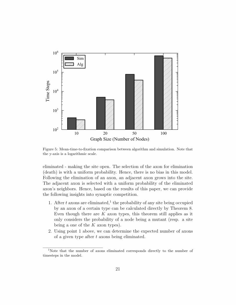
We generated random (ER) graphs of size 10, 20, 50 and 100 nodes, creat-ing five different graphs for each number of nodes. The graphs were generatedas in our convergence experiments, and our comparison to Monte Carlo test-ing are shown in Figure 5 where we demonstrate experimentally that ouralgorithm produces a lower bound. Our algorithm was run until the stan-dard deviation of fixation probabilities for all vertices was 2.5 × 10−6. TheMonte Carlo simulations were each set at 10, 000 runs.

8. Application: Competition Among Neural Axons

In recent work, [26] created a model for synaptic competition based ondeath-birth updating under neutral drift. They noted that the model alignswell with their empirical observations. In the model, the graph represents asynaptic junction and the nodes represent sites in the junction. For every twoadjacent sites in the synaptic junction, there is an undirected edge betweenthe corresponding two nodes in the graph. Hence, in- and out- degrees ofeach node are the same. Initially, there are K different axon types locatedin the junction configured in a manner where all sites are initially occupiedby one axon type. At each time step, an axon occupying one of the sites is

20

10 20 50 100Graph Size (Number of Nodes)

102

103

104

105

106Ti

me

Step

s

SimAlg

Figure 5: Mean-time-to-fixation comparison between algorithm and simulation. Note thatthe y-axis is a logarithmic scale.

eliminated - making the site open. The selection of the axon for elimination(death) is with a uniform probability. Hence, there is no bias in this model.Following the elimination of an axon, an adjacent axon grows into the site.The adjacent axon is selected with a uniform probability of the eliminatedaxon’s neighbors. Hence, based on the results of this paper, we can providethe following insights into synaptic competition.

1. After t axons are eliminated,1 the probability of any site being occupiedby an axon of a certain type can be calculated directly by Theorem 8.Even though there are K axon types, this theorem still applies as itonly considers the probability of a node being a mutant (resp. a sitebeing a one of the K axon types).

2. Using point 1 above, we can determine the expected number of axonsof a given type after t axons being eliminated.

1Note that the number of axons eliminated corresponds directly to the number oftimesteps in the model.

21

3. After t axons are eliminated, the probability of any set of sites beingoccupied by a certain axon type is simply the sum of the probabilitiesof the individual sites being occupied by that axon. As a result, thefixation probability is additive.

4. Leveraging point 3 above combined with an easy modification of theresult of Broom et al. [6] for the BD model, the fixation probabilityof an axon originating at site i is ki

2·Θ where ki is the number of sitesadjacent to site i (hence the degree of node i in the correspondinggraph) and Θ is the total number of adjacencies in the synapse (hence,half the number of directed edges in the corresponding graph).

5. Based on item 4 above and the results from Section 3, we can concludethat for a given axon type (let’s call it “axon type A”) occupying aset of sites, that if the average adjacencies of those sites is greaterthan (resp. less than) the overall average adjacencies for the sites inthe entire synaptic junction, then as the number of eliminated axonsapproaches infinity, we can expect the number of axon type A in thesynaptic junction will increase (resp. decrease) in expectation.

6. We can directly apply Theorem 7 to find a lower-bound on the numberof eliminated axons before fixation occurs.

We note that the results stated above are either precise mathematical ar-guments or calculations that can be found exactly with a deterministic al-gorithm. They are not theoretical approximations and do not rely on sim-ulation. As such is the case, we can make more precise statements aboutsynaptic competition (given the model) and can avoid the variance thataccompanies simulation results. Insights such as these may lead to futurebiological experiments.

9. Related Work

Evolutionary graph theory was originally introduced in [14]. Previously,we have compiled a comprehensive review [24] for a general overview of thework in this exciting new area.

While most work dealing with evolutionary graphs rely on Monte Carlosimulation, there are some good analytical approximations for the undi-rected/unweighted cased based on the degree of the vertices in question.Antal et al. [1] use the mean-field approach to create these approximationsfor the undirected/unweighted case. Broom et al. [6] derive an exact analyt-ical result for the undirected/unweighted case in neutral drift, which agrees

22

with the results of Antal et al. They also show that fixation probability isadditive in that case (a result which we extend in this paper using a differentproof technique). However, the results of [16] demonstrate that mean-fieldapproximations break down in the case of weighted, directed graphs. [15]also studied weighted, directed graphs, but does so by using Monte Carlosimulation. [22] derive exact computation of fixation probability throughmeans of linear programming. However, that approach requires an exponen-tial number of both constraints and variables and is intractable. The recentwork of [27] introduces a parameter called graph determinacy which mea-sures the degree to which fixation or extinction is determined while startingfrom a randomly choses initial configuration. This property is then usedto analyze some special cases of evolutionary graphs under birth-death up-dating. There has been some work on algorithms for fixation probabilitycalculation that rely on a randomized approach [4, 9]. [4] present a heuris-tic technique for speeding up Monte Carlo simulations by early terminationwhile [9] present utilize simulation runs in a fully-polynomial randomizedapproximation scheme. However, our framework differs in that it does notrely on simulation at all and provides a deterministic result. Further, ournon-randomized approach also allows for additional insights into the evolu-tionary process - such as monitoring the expected number of mutants as afunction of time. Recently, [12] study the related problem of determining theprobability of fixation given a single, randomly placed mutant in the graphwhere the vertices are “islands” and there are many individuals residing oneach island in a well-mixed population. They use quasi-fixed points of ODE’sto obtain an approximation of the fixation probability and performed experi-ments with a maximum of 5 islands (vertices) containing 50 individuals each.This continuous approximation provides the best results when the numberof individuals in each island is much larger than the number of islands. Asthe problem of this paper can be thought of as a special case where eachisland has just one individual, it seems unlikely that the approximation ofHouchmandzadeh and Vallade’s approach will hold here.

Some of the results in this paper were previously presented in conferencesby the authors [23, 17]. The analysis and experiments concerning the ex-pected number of mutants at a given time, the extension of the frameworkfor other update rules (beyond birth-death), the use of the framework for thecase of r > 1, and the neurology applications are all new results appearingfor the first time in this paper.

23

10. Conclusion

In this paper, we introduced a new approach to deal with problems relat-ing to evolutionary graphs that rely on “vertex probabilities.” Our presentedanalytical method is the first deterministic method to compute fixation prob-ability and provides a number of novel uses and results for EGT problems:

• Our method can be used to solve for the fixation probability underneutral drift orders of magnitude faster than Monte Carlo simulations,which is currently the presiding employed method in EGT studies. Wehave extended the method to all of the commonly used update pro-cesses in EGT. The special case of neutral drift is not only of interestin the literature [6, 15] but also it has been applied to problems inneurology [26].

• While the presented method is currently constrained to the case ofneutral drift, we have demonstrated how it can inform cases of non-neutral drift by using it to provide both a lower and upper bound forthis case. Combined with our analytical method’s speed, this meansthat it can be used to acquire useful knowledge to guide general EGTstudies interested in the case of advantageous mutants.

• We have shown how our analytical method can be used to calculate anon-trivial lower bound to the mean time to fixation, providing a firststep for a general method to computing this and related quantities thatis lacking in the current literature.

• We have shown how our method can be used to calculate deterministi-cally the expected number of mutants, which is useful for applicationsthat require predictions on the number of mutants in the populationunder a specific finite time horizon. We have also provided results onthe expected number of mutants on different common graph topologies,showing differences in the growth trajectories of amplifiers and sup-pressors on these different topologies. These results may prove highlysignificant in the recent application of EGT to distributed systems [13]where the problem of information diffusion is considered among com-puter systems. In such a domain, it may be insufficient to guaranteefixation in the limit of time - which may be impractical - but rather tomake guarantees on the outcome of the process after a finite amountof time.

24

• Finally, we have shown how our method can provide insight when ap-plied to the problem of synaptic competition in neuroscience.

Though evolutionary graph theory is still a relatively new research area, itis actively being studied in a variety of disciplines [14, 24, 28, 25, 20, 26, 13].We believe that more real-world applications will appear as this area gainsmore popularity. As illustrated by recent work [26, 13], experimental sci-entists with knowledge of EGT may be more likely to recognize situationswhere the model may be appropriate. As these cases arise, deterministicmethods for addressing issues related to EGT may prove to be highly useful.However, this paper is only a starting point - there are still many impor-tant directions for future work. Foremost among such topics are scenarioswhere the topology of the graph also changes over time or where additionalattributes of the nodes/edges in the graph affect the dynamics.

Acknowledgments

P.S. is supported by ARO projects 611102B74F and 2GDATXR042 as well asOSD project F1AF262025G001. P.R. is supported by ONR grant W911NF0810144.P.S. would like to thank Stephen Turney (Harvard University) for severaldiscussions concerning his work. The opinions in this paper are those of theauthors and do not necessarily reflect the opinions of the funders, the U.S.Military Academy, the U.S. Army, or the U.S. Navy.

References

1 Antal, T., Redner, S., Sood, V., 2006. Evolutionary dynamics on degree-heterogeneous graphs. Physical Review Letters 96 (18), 188104.

2 Antal, T., Scheuring, I., 2006. Fixation of strategies for an evolutionarygame in finite populations. Bulletin of Mathematical Biology 68, 1923–1944.

3 Barabasi, A., Albert, R., 1999. Emergence of scaling in random networks.science 286 (5439), 509–512.

4 Barbosa, V. C., Donangelo, R., Souza, S. R., Oct 2010. Early appraisalof the fixation probability in directed networks.

25

5 Broom, M., Hadjichrysanthou, C., Rychtar, J., 2009. Evolutionary gameson graphs and the speed of the evolutionary process. Proceedings of theRoyal Society A.

6 Broom, M., Hadjichrysanthou, C., Rychtar, J., Stadler, B. T., Apr. 2010.Two results on evolutionary processes on general non-directed graphs.Proceedings of the Royal Society A: Mathematical, Physical and Engi-neering Sciences 466 (2121), 2795–2798.

7 Broom, M., Rychtar, J., May 2009. An analysis of the fixation probabilityof a mutant on special classes of non-directed graphs. Proceedings of theRoyal Society A 464, 2609–2627.

8 Broom, M., Rychtar, J., Stadler, B., 2011. Evolutionary dynamics ongraphs - the effect of graph structure and initial placement on mutantspread. Journal of Statistical Theory and Practice 5 (3), 369–381.

9 Dıaz, J., Goldberg, L., Mertzios, G., Richerby, D., Serna, M., Spirakis,P., Jan. 2012. Approximating Fixation Probabilities in the GeneralizedMoran Process. In: Proceedings of the ACM-SIAM Symposium on Dis-crete Algorithms (SODA), Kyoto, Japan. ACM.

10 Erdos, P., Renyi, A., 1960. On the evolution of random graphs. Akad.Kiado.

Hagberg et al. Hagberg, Aric A. and Schult, Daniel A. and Swart, Pieter J..Exploring network structure, dynamics, and function using NetworkX. InProceedings of the 7th Python in Science Conference (SciPy2008), pages11–15, Pasadena, CA USA, August 2008.

12 Houchmandzadeh, B., Vallade, M., July 2011. The fixation probabilityof a beneficial mutation in a geographically structured population. NewJournal of Physics 13 (7), 073020.URL http://stacks.iop.org/1367-2630/13/i=7/a=073020

13 Jiang, C., Chen, Y. C., Liu, K. J. R., Dec 2012. Distributed Adap-tive Networks: A Graphical Evolutionary Game-Theoretic View. arXiv:1212.1245.

14 Lieberman, E., Hauert, C., Nowak, M. A., 2005. Evolutionary dynamicson graphs. Nature 433 (7023), 312–316.

26

15 Masuda, N., 2009. Directionality of contact networks suppresses selectionpressure in evolutionary dynamics. Journal of Theoretical Biology 258 (2),323 – 334.

16 Masuda, N., Ohtsuki, H., 2009. Evolutionary dynamics and fixation prob-abilities in directed networks. New Journal of Physics 11 (3), 033012(15pp).

17 Moores, G., Shakarian, P., 2012. A fast and deterministic method formean time to fixation in evolutionary graphs. Presented at INSNA Sun-belt XXXII, Redondo Beach, CA.

18 Moran, P., 1958. Random processes in genetics. Mathematical Proceed-ings of the Cambridge Philosophical Society 54 (01), 60–71.

19 Newman, M., Watts, D., 1999. Renormalization group analysis of thesmall-world network model. Physics Letters A 263 (4-6), 341–346.

20 Pacheco, J. M., Traulsen, A., Nowak, M. A., December 2006. Activelinking in evolutionary games. Journal of Theoretical Biology 243 (3),437–443.

21 Paley, C. J., Taraskin, S. N., Elliott, S. R., 2007. Temporal and dimen-sional effects in evolutionary graph theory. Physical Review Letters 98,098103.

22 Rychtar, J., Stadler, B., Winter 2008. Evolutionary dynamics on small-world networks. International Journal of Computational and Mathemat-ical Sciences 2 (1).

23 Shakarian, P., Roos, P., Nov. 2011. Fast and deterministic computationof fixation probability in evolutionary graphs. In: CIB ’11: The SixthIASTED Conference on Computational Intelligence and Bioinformatics.IASTED.

24 Shakarian, P., Roos, P., Johnson, A., 2012. A review of evolutionarygraph theory with applications to game theory. Biosystems 107 (2), 66 –80.URL http://www.sciencedirect.com/science/article/pii/S0303264711001675

27

25 Sood, V., Antal, T., Redner, S., 2008. Voter models on heterogeneousnetworks. Physical Review E 77 (4), 041121.

26 Turney, S., Lichtman, J., June 2012. Reverseing the outcome of synapseelimination at devloping neuromuscular junction in vivo: Evidence forsynapcitc competition and its mechansm. PLoS Biology 10.

27 Voorhees, B., 2012. Birth-Death Fixation Probabilities for StructuredPopulations. Proceedings of the Royal Society A: Mathematical, Physicaland Engineering Sciences (accepted).

28 Zhang, P. A., Nie, P. Y., Hu, D. Q., Zou, F. Y., 2007. The analysis ofbi-level evolutionary graphs. Biosystems 90 (3), 897–902.

28

Supplementary Material

11. Notes

Throughout this supplement, we will use an extended notation. Fixationprobability given initial configuration C is denoted FC . For vertex i at timet, we denote this as Pr(M(t)

i ). We will use S(t)i to denote the event that vertex

i was selected for reproduction and R(t)ij to denote the event of i replacing

j. We will often use conditional probabilities. For example, Pr(M(t)i |C(0))

is the probability that vi is a mutant given the initial set C of mutants.Throughout this supplement, unless noted otherwise, all of our probabili-ties will be conditioned on C(0). We will drop it for ease of notation withthe understanding that some set C of V were mutants at t = 0. Hence,Pr(M(t)

i ) = Pr(M(t)i |C(0)).

12. Proof of Theorem 1

∀i, limt→∞Pr(M(t)i |C(0)) = FC

Proof. Consider the following definition property of Pr(M(t)i |C(0))

Pr(M(t)i |C(0)) =

∑V ′∈2V

s.t. vi∈V ′

Pr(V ′(t)|C(0)) (16)

We note that as time approaches infinity, for all V ′ ∈ 2V − ∅ − V we havePr(V ′(t)|C(0)) = 0. As vi /∈ ∅, the statement follows. Q.E.D.

13. Proof of Theroem 2

Pr(M(t)i ) =

Pr(M(t−1)i ) +

∑(vj ,vi)∈E

wji ·Pr(M(t−1)j ) ·Pr(S(t)

j |M(t−1)j )− wji ·Pr(M(t−1)

i ) ·Pr(S(t)j |M

(t−1)i )

Where S(t)i is true iff vi is selected for reproduction at time t.

29

Proof. Note we use the variable R(t)j i is true iff vj replaces vi at time t.

CLAIM 1:

Pr(M(t)i ) = Pr(M(t−1)

i ∧∧

(vj ,vi)∈E

¬S(t)j ) +

∑(vj ,vi)∈E

Pr(S(t)j ∧ R(t)

ji ∧M(t−1)j ) +

∑(vj ,vi)∈E

Pr(S(t)j ∧ ¬R

(t)ji ∧M(t−1)

i )

This is shown by a simple examination of exhaustive and mutually exclusiveevents based on the original model of [14].

CLAIM 2:

Pr(M(t−1)i ∧

∧(vj ,vi)∈E

¬S(t)j ) = Pr(M(t−1)

i ) ·

1−∑

(vj ,vi)∈E

Pr(S(t)j |M

(t−1)i )

(Proof of claim 2) By exhaustive and mutual exclusive events, we have thefollowing.

Pr(M(t−1)i ∧

∧(vj ,vi)∈E

¬S(t)j ) = Pr(M(t−1)

i )−∑

(vj ,vi)∈E

Pr(S(t)j ∧M(t−1)

i )

By the definition of conditional probability, we have the following

Pr(M(t−1)i ∧

∧(vj ,vi)∈E

¬S(t)j ) = Pr(M(t−1)

i )−∑

(vj ,vi)∈E

(Pr(S(t)

j |M(t−1)i ) ·Pr(M(t−1)

i ))

= Pr(M(t−1)i )−Pr(M(t−1)

i ) ·∑

(vj ,vi)∈E

Pr(S(t)j |M

(t−1)i )

= Pr(M(t−1)i )

1−∑

(vj ,vi)∈E

Pr(S(t)j |M

(t−1)i )

The claim immediately follows.

CLAIM 3: For all edges (vj, vi), we have the following.

Pr(S(t)j ∧ R(t)

ji ∧M(t−1)j ) = wji ·Pr(M(t−1)

j ) ·Pr(S(t)j |M

(t−1)j )

30

(Proof of claim 3) The following is a direct application of the definition ofconditional probability.

Pr(S(t)j ∧ R(t)

ji ∧M(t−1)j ) = Pr(R(t)

ji ∧M(t−1)j |S(t)

j ) ·Pr(S(t)j )

From our model, we note that given even S(t)j , the fitness of the nodes is not

considered in determining if the event associated with R(t)ji is to occur. Hence,

it follows that M(t−1)j is independent of R(t)

ji given S(t)j . As Pr(R(t)

ji |S(t)j ) = wji,

we have the following.

Pr(S(t)j ∧ R(t)

ji ∧M(t−1)j ) = Pr(R(t)

ji |S(t)j ) ·Pr(M(t−1)

j |S(t)j ) ·Pr(S(t)

j )

= wji ·Pr(M(t−1)j |S(t)

j ) ·Pr(S(t)j )

By Bayes Theorem, and that the model causes ∀iPr(S(t)i ) > 0, we have the

following.

Pr(S(t)j ∧ R(t)

ji ∧M(t−1)j ) = wji ·Pr(S(t)

j |M(t−1)j ) ·

Pr(M(t−1)j )

Pr(S(t)j )

·Pr(S(t)j )

= wji ·Pr(M(t−1)j ) ·Pr(S(t)

j |M(t−1)j )

The claim follows immediately.

CLAIM 4: For all edges (vj, vi), we have the following.

Pr(S(t)j ∧ ¬R

(t)ji ∧M(t−1)

i ) = (1− wji) ·Pr(M(t−1)i ) ·Pr(S(t)

j |M(t−1)i )

(Proof of claim 4) This mirrors claim 3.

(Proof of theorem) From claims 1-4, we have the following.

Pr(M(t)i ) = Pr(M(t−1)

i ) ·

1−∑

(vj ,vi)∈E

Pr(S(t)j |M

(t−1)i )

+ (17)

∑(vj ,vi)∈E

(wji ·Pr(M(t−1)

j ) ·Pr(S(t)j |M

(t−1)j )

)+ (18)

∑(vj ,vi)∈E

((1− wji) ·Pr(M(t−1)

i ) ·Pr(S(t)j |M

(t−1)i )

)(19)

Which, after re-arranging some terms, gives us the statement of the theorem.Q.E.D.

31

14. Proof of Theorem 3

When r = 1, if for some time t, ∀i, the value Pr(M(t)i ) is the same, then

Pr(M(t)i ) = FC .

Proof Sketch. Consider Pr(M(t)i ) = Pr(M(t−1)

i )+ 1N

∑(vj ,vi)∈E wji·(Pr(M(t−1)

j )−Pr(M(t−1)

i )) when for t−1, ∀i, j we have Pr(M(t−1)j ) = Pr(M(t−1)

i ). Clearly,

in this case, the value for Pr(M(t)i ) = Pr(M(t−1)

i ). As the probabilities of allvertices was the same at t− 1, they remain so at t. Therefore, in this case,limt→∞Pr(M(t)

i ) = Pr(M(t)i ). QED

15. Proof of Inequality 4

For any time t, under neutral drift (r = 1),

mini

Pr(M(t)i ) ≤ FC ≤ max

iPr(M(t)

i )

Proof. PART 1: For any time t, under neutral drift (r = 1), FC ≤maxiPr(M(t)

i ).

We show that for each time step t, maxiPr(M(t−1)i ) ≥ maxiPr(M(t)

i ). Hence,

by showing that, for any time t′, we have maxiPr(M(t′)i ) ≥ limt→∞maxiPr(M(t)

i )which by allows us to apply Theorem 1 and obtain the statement of this theo-rem. Suppose BWOC that at time t we have max`Pr(M(t−1)

` ) < maxiPr(M(t)i ).

32

Then we have:

max`

Pr(M(t−1)` ) <

1

N

∑(vj ,vi)∈E

wji ·(Pr(M(t−1)

j )−Pr(M(t−1)i )

)+Pr(M(t−1)

i )

≤ 1

N

∑(vj ,vi)∈E

wji ·(

max`

Pr(M(t−1)` )−Pr(M(t−1)

i ))

+Pr(M(t−1)i )

=

∑(vj ,vi)∈E wji

N

(max`

Pr(M(t−1)` )−Pr(M(t−1)

i ))

+Pr(M(t−1)i )

max`

Pr(M(t−1)` )(1−

∑(vj ,vi)∈E wji

N) < Pr(M(t−1)

i )(1−∑

(vj ,vi)∈E wji

N)

max`

Pr(M(t−1)` ) < Pr(M(t−1)

i )

Which is clearly a contradiction and completes this part of the proof.PART 2: For any time t, under neutral drift (r = 1), FC ≥ miniPr(M(t)

i ).

We show that for each time step t, miniPr(M(t−1)i ) ≤ miniPr(M(t)

i ). Hence,

by showing that, for any time t′, we have miniPr(M(t′)i ) ≤ limt→∞maxiPr(M(t)

i )which by allows us to apply Theorem 1 and obtain the statement of this theor-erm. Suppose BWOC that at time t we have min`Pr(M(t−1)

` ) > miniPr(M(t)i ).

33

Then we have:

min`

Pr(M(t−1)` ) >

1

N

∑(vj ,vi)∈E

wji ·(Pr(M(t−1)

j )−Pr(M(t−1)i )

)+Pr(M(t−1)

i )

≥ 1

N

∑(vj ,vi)∈E

wji ·(

min`

Pr(M(t−1)` )−Pr(M(t−1)

i ))

+Pr(M(t−1)i )

=

∑(vj ,vi)∈E wji

N

(min`

Pr(M(t−1)` )−Pr(M(t−1)

i ))

+Pr(M(t−1)i )

min`

Pr(M(t−1)` )(1−

∑(vj ,vi)∈E wji

N) > Pr(M(t−1)

i )(1−∑

(vj ,vi)∈E wji

N)

min`

Pr(M(t−1)` ) > Pr(M(t−1)

i )

Which is clearly a contradiction and completes this part of the proof. Q.E.D.

16. Proof of Theorem Theorem 4

When r = 1 for disjoint sets C,D ⊆ V , FC + FD = FC∪D.Proof. Consider some time t and vertex vi. Clearly, by Corollary 1, Pr(M(t)

i )

can be expressed as a linear combination of the form∑

vj∈V (Cj · Pr(M(0)j ))

where Cj is a coefficient. We note that these coefficients are the same re-

gardless of the initial configuration of mutants that M(t)i is conditioned on.

Hence, Pr(M(t)i |C(0)) is this positive function with Pr(M(0)

j ) = 1 if vj ∈ Cand 0 otherwise (see Proposition 3). Hence, for disjoint C,D, for any vi ∈ V ,

we have Pr(M(t)i |C(0))+Pr(M(t)

i |D(0)) = Pr(M(t)i |(C∪D)(0)). The statement

follows. Q.E.D.

17. Proof of Equation 9

Pr(M(t)i ) =

(1− 1

N

)·Pr(M(t−1)

i ) +1

N · k(i)in

∑(vj ,vi)∈E

Pr(M(t−1)j )

34

Under death-birth dynamics with neutral drift (r = 1).

Proof. D(t)i and B(t)

i are random variables associated with birth and deathevents for vertex vi.CLAIM 1: Pr(M(t)

i ) = Pr(M(t−1)i ∧¬D(t)

i )+∑

(vj ,vi)∈E Pr(D(t)i ∧B

(t)j ∧M

(t−1)j )

Follows directly form exhaustive and mutually exclusive events.CLAIM 2: Pr(M(t−1)

i ∧ ¬D(t)i ) =

(1− 1

N

)·Pr(M(t−1)

i )

By the definition of conditional probabilities, we have Pr(¬D(t)i |M

(t−1)i ) ·

Pr(M(t−1)i ). Also, we know the probability of a given node dying is always

1/N . Hence, Pr(¬D(t)i |M

(t−1)i ) = Pr(¬D(t)

i ) = 1− 1N

and the claim follows.CLAIM 3: For any (vj, vi) ∈ E, we have

Pr(D(t)i ∧ B(t)

j ∧M(t−1)j ) = 1

N ·k(i)in

·Pr(M(t−1)j )

As both birth and death events occur independent of any node being a mutantat the previous time step, the definition of conditional probabilities gives usthe following:

Pr(D(t)i ∧ B(t)

j ∧M(t−1)j ) = Pr(D(t)

i ∧ B(t)j ) ·Pr(M(t−1)

j ) (20)

= Pr(B(t)j |D

(t)i ) ·Pr(D(t)

i ) ·Pr(M(t−1)j ) (21)

From the model, we have the following:

Pr(B(t)j |D

(t)i ) = 1/k

(i)in (22)

Pr(D(t)i ) = 1/N (23)

Hence, the claim follows. QED Q.E.D.

18. Proof of Equation 10

Pr(M(t)i ) =

(1− k

(i)in

|E|

)·Pr(M(t−1)

i ) +1

|E|∑

(vj ,vi)∈E

Pr(M(t−1)j )

Under link dynamics with neutral drift (r = 1).

Proof. Here S(t)ij is the random variable associated with the selection of edge

(vi, vj).

CLAIM 1: Pr(M(t)i ) = Pr(M(t−1)

i ∧∧

(vj ,vi)∈E ¬S(t)ji ) +

∑(vj ,vi)∈E Pr(S(t)

ji ∧M(t−1)

j )

35

Follows directly form exhaustive and mutually exclusive events.

CLAIM 2: Pr(∧

(vj ,vi)∈E ¬S(t)ji ) = 1− k

(i)in

|E|

Clearly, we have Pr(∧

(vj ,vi)∈E ¬S(t)ji ) = Pr(

∨{(vβ ,vα)∈E|β 6=i} S

(t)βα). As there are

k(i)in incoming edges to vi, we know that Pr(

∨{(vβ ,vα)∈E|β 6=i} S

(t)βα) = 1 − k

(i)in

|E| ,giving us the claim.

CLAIM 3: Pr(M(t−1)i ∧

∧(vj ,vi)∈E ¬S

(t)ji ) =

(1− k

(i)in

|E|

)·Pr(M(t−1)

i )

For any α, β, the random variable S(t)αβ is independent from M(t−1)

i . Hence,the claim immediately follows from this fact and claim 2.CLAIM 4: Pr(S(t)

ji ∧M(t−1)j ) = 1

|E| ·Pr(M(t−1)j )

As, by the definition of the model, Pr(S(t)ji |M

(t−1)j ) = Pr(S(t)

ji ) = 1|E| , the

claim follows directly form the definition of conditional probabilities. QEDQ.E.D.

19. Proof of Theorem 5

For a given set C, let F (1)(C) be the fixation probability under neutraldrift and F (r)(C) be the fixation probability calculated using a mutant fitnessr > 1. Then, under BD-B, BD-D, DB-B, DB-D, or LD dynamics, F (1)(C) ≤F (r)(C).Proof. First, some notation.

• We define an interpretation, I : 2V → [0, 1] as probability distributionover mutant configurations. Hence, for some I we have

∑V ′∈2V I(V ′) =

1.

• Next, we define a transition function that maps configurations of mu-tants to probabilities, χ : 2V → [0, 1] where for any C ∈ 2V ,

∑C′∈2V χ(C,C ′) =

1. We will use χ+ and χ− to indicate if the transition is made with amutant being selected for birth (χ+) or resident (χ−). Hence, for someC ∈ V and v /∈ C, χ−(C,C ∪{v}) = 0 and χ+(C ∪{v}, C) = 0. Hence,for all C ∈ 2V ,

∑C′∈2V (χ+(C,C ′) + χ−(C,C ′)) = 1.

• If the transitioon function is based on birth-death and computed withsome r > 1, then we will write it as χ

(r)+ , χ

(r)− respectively. If computed

with r = 1, then we write χ(nd)+ , χ

(nd)− respectively.

36

• For some C ∈ 2C , let inc(C) be the set of all elements D ∈ 2V s.t.|D| ≥ |C| and χ+(C,D) > 0.

• For some C ∈ 2C , let dec(C) be the set of all elements D ∈ 2V s.t.|D| ≤ |C| and χ−(C,D) > 0.

• Given set C ⊆ V , we will use F(r)C to denot the probability of fixation

given initial set of mutants C where the value r is used to calculate alltransition probabilities.

CLAIM 1: If a some time period, the probability distribution over mutantconfigurations is I, the fixation probability is

∑C∈2V I(C) · F (r)

C .

Clearly, for any time t, F(r)C = lim i→∞Pr(V (i)|C(t)). Under the assump-

tion that there exists some tim ω s.t. fixation is reached, we have:

F(r)C = Pr(V (ω)|C(t))

=Pr(V (ω) ∧ C(t))

Pr(C(t))

Hence, F(r)C ·Pr(C(t)) = Pr(V (ω) ∧ C(t)). The statement then follows by the

summation of exhaustive and mutually exclusive events.

CLAIM 2: If a some time period t, the probability distribution over mutantconfigurations is I, and the transition functions used to reach the next timestep are χ+, χ−, then the probability of being in some mutant configurationC at time t+ 1 is given by

∑D∈2V I(D) · (χ+(D,C) + χ−(D,C)).

Follows directly from the rules of dynamics.

CLAIM 3: If a some time period t, the probability distribution over mu-tant configurations is I, mutant fitness r, and the transition functions usedto reach the next time step are χ

(r)+ , χ

(r)− , and all subsequent transitions are

computed using the same dynamics with neutral drift, then the fixation prob-ability is:

P(I, r) =∑C∈2V

I(C) ·

∑D∈inc(C)

(χ(r)+ (C,D) · F (1)

D ) +∑

D∈dec(C)

(χ(r)− (C,D) · F (1)

D ))

37

Follows directly from claims 1-2.

CLAIM 4: Under BD-B, BD-D, DB-B, DB-D, or LD dynamics, for some

r ≤ r′, for all C,D ∈ 2V , we have χ(r)+ (C,D) ≤ χ

(r′)+ (C,D) and χ

(r)− (C,D) ≥

χ(r′)− (C,D).

CLAIM 4a: For some r ≤ r′, for all C,D ∈ 2V , we have χ(r)+ (C,D) ≤

χ(r′)+ (C,D).

Let {vj} = D−C. For each vertex vi, fi = 1 if vi /∈ C (a resident) and fi = rif vi ∈ C (a mutant). When D ≡ C, the following are all summed over theset {vj ∈ C|∃vi ∈ C ∧ (vi, vj) ∈ E}.

• Under BD-B,

χ(r)+ (C,D) =

∑vi∈C|

(vi,vj)∈E

r · wijr · |C|+N − |C|

• Under BD-D, ∑vi∈C|

(vi,vj)∈E

wijN ·

∑vq |(vi,vq)∈E wiq · f−1

q

• Under DB-B,

χ(r)+ (C,D) =

∑vi∈C|

(vi,vj)∈E

wij · rN ·

∑vq |(vq ,vj)∈E wqj · fq

• Under DB-D,

χ(r)+ (C,D) =

∑vi∈C|

(vi,vj)∈E

wij∑vq∈V f

−1q

• Under LD,

χ(r)+ (C,D) =

∑vi∈C|(vi,vj)∈E

wij · r∑vq ,v`|(vq ,v`)∈E wq` · fq

38

By simple algebraic manipulation, for each of these, when all values otherthan r are fixed, they increase as r increases.

CLAIM 4b: For some r ≤ r′, for all C,D ∈ 2V , we have χ(r)− (C,D) ≥

χ(r′)− (C,D). Let {vj} = C − D. For each vertex vi, fi = 1 if vi /∈ C (a

resident) and fi = r if vi ∈ C (a mutant). When D ≡ C, the following areall summed over the set {vj ∈ V − C|∃vi ∈ V − C ∧ (vi, vj) ∈ E}.

• Under BD-B,

χ(r)+ (C,D) =

∑vi∈V−C|(vi,vj)∈E

wijr · |C|+N − |C|

• Under BD-D, ∑vi∈V−C|(vi,vj)∈E

wij · r−1

N ·∑

vq |(vi,vq)∈E wiq · f−1q

• Under DB-B,

χ(r)+ (C,D) =

∑vi∈V−C|(vi,vj)∈E

wijN ·

∑vq |(vq ,vj)∈E wqj · fq

• Under DB-D,

χ(r)+ (C,D) =

∑vi∈V−C|(vi,vj)∈E

wij · r−1∑vq∈V f

−1q

• Under LD,

χ(r)+ (C,D) =

∑vi∈V−C|(vi,vj)∈E

wij∑vq ,v`|(vq ,v`)∈E wq` · fq

39

By simple algebraic manipulation, for each of these, when all values otherthan r are fixed, they decrease as r increases.

CLAIM 5: Given some C ∈ 2V , for all pairs D,D′ where D ∈ inc(C) and

D′ ∈ dec(C), we have F(1)D ≥ F

(1)D′ .

Follows directly from Theorem 5.

CLAIM 6: Given interpretation I, under BD-B, BD-D, DB-B, DB-D, or LDdynamics, for some r > 1, P(I, r) ≥ P(I, 0).Let us consider some set C from the outermsot summation in the computa-tion of P(I, r). Suppose, BWOC, there exists some C ∈ 2V s.t.:

∑D∈inc(C)

(χ(r)+ (C,D) · F (1)

D ) +∑

D∈dec(C)

(χ(r)− (C,D) · F (1)

D ) <∑

D∈inc(C)

(χ(1)+ (C,D) · F (1)

D ) +∑

D∈dec(C)

(χ(1)− (C,D) · F (1)

D )

This give us:

∑D∈inc(C)

(χ(r)+ (C,D) · F (1)

D )−∑

D∈inc(C)

(χ(1)+ (C,D) · F (1)

D ) <∑

D∈dec(C)

(χ(1)− (C,D) · F (1)

D )−∑

D∈dec(C)

(χ(r)− (C,D) · F (1)

D )

Let Fsm = inf {F (1)D |D ∈ inc(C)} and Flg = sup{F (1)

D |D ∈ dec(C)}, this giveus:

Fsm∑

D∈inc(C)

(χ(r)+ (C,D)− χ(1)

+ (C,D)) < Flg∑

D∈dec(C)

(χ(1)− (C,D)− χ(r)

− (C,D))

Consider ther following:

∑D∈inc(C)

χ(r)+ (C,D) +

∑D∈dec(C)

χ(r)− (C,D) =

∑D∈inc(C)

χ(1)+ (C,D) +

∑D∈dec(C)

χ(1)− (C,D)

∑D∈inc(C)

χ(r)+ (C,D)−

∑D∈inc(C)

χ(1)+ (C,D) =

∑D∈dec(C)

χ(1)− (C,D)−

∑D∈dec(C)

χ(r)− (C,D)

Note that by claim 4, both sides of the above equation are positive numbers.Hence, we have Fsm < Flg, which contradicts claim 5.

PROOF OF THEOREM: Let P(1)(I, r) = P(I, r) and P(i+1)(I, r) = P(P(i)(I, r), r).By claim 6, for any i, P(i+1)(I, r) ≥ P(P(i)(I, r), r). Consider an inter-pretation I that describes the initial probability distribution over mutantconfigurations. The fixation probability under neutral drift is P(I, 1). Forsome value r > 1, the fixation probaiblity is lim i→∞P(i)(I, r). Clearly,lim i→∞P(i)(I, r) ≥ P(I, 1). Q.E.D.

40

20. Proof of Theorem 6

tC =1

FC

∞∑t=1

t · (Ft|C − Ft−1|C)

Proof. This proof was first presented in [2]. The mean time to fixation isdescribed as the expected time to fixation given that the process fixates. LetFt|C be the probability that fixation is reached in exactly t time-steps or less.Hence, the probability of reaching fixation in exactly t time steps conditionedon the process reaching fixation is (Ft|C − Ft−1|C)/FC . The remainder of thetheorem follows from the definition of an expected value. Q.E.D.

21. Proof of Theorem 7

We introduce two pieces of notation tfix, tconvg. We define tfix as a time

s.t. tC = 1FC

∑tfixt=1 t · (Ft|C − Ft−1|C). and tconvg s.t. ∀i, Pr(M

(tconvg)i ) = FC .

While in reality, both of these values could be infinite, we note that therelationship ∞ ≥ tfix ≥ tconvg holds and that using a lower value for tfixand/or tconvg will still ensure we have a lower bound.

1

FC

∞∑t=1

t · (Pmin,t − Pmin,t−1) ≤ 1

FC

∞∑t=1

t · (Ft|C − Ft−1|C)

Where Pmin,t = miniPr(M(t)i ).

Proof. First, we have the following.

tconvg∑t=1

t · (Pmin,t − Pmin,t−1) ≤tfix∑t=1

t · (Ft|C − Ft−1|C) (24)

For any time t, let P(t)C = Ft|C − Ft−1|C and Pr(∆M(t)

min) = Pmin,t − Pmin,t−1.

As for each time t, we have Pmin,t ≥ Ft|C , we can define θ(t)t′ as the portion of

P(t)C accounted for in Pr(∆M(t′)

min). This results in having θ(t)t′ = 0 whenever

41

t′ > t or t > tconvg as well as the following:

P(t)C =

t∑t′=1

θ(t)t′ (25)

Pr(∆M(t)min) =

tfix∑t′=t

θ(t′)t (26)

tconvg∑t=1

t · (Pmin,t − Pmin,t−1) =

tconvg∑t=1

tfix∑t′=t

tθ(t′)t (27)

=

tconvg∑t=1

tfix∑t′=1

tθ(t′)t (28)

=

tfix∑t′=1

tconvg∑t=1

tθ(t′)t (29)

=

tfix∑t′=1

t′∑t=1

tθ(t′)t (30)

We also note that the following is true:

tfix∑t=1

t · (Ft|C − Ft−1|C) =

tfix∑t′=1

t′P(t′)C (31)

=

tfix∑t′=1

t′t′∑t=1

θ(t′)t (32)

≥tfix∑t′=1

t′∑t=1

tθ(t′)t (33)

=

tconvg∑t=1

t · (Pmin,t − Pmin,t−1) (34)

Which concludes the proof. Q.E.D.

22. Materials and Methods

Except for the experiments dealing with time to fixation/extinction, allalgorithms were implemented in Python and run on a 2.33GHz Intel Xeon

42

CPU. The time-to-fixation experiments were run on a machine equipped withan Intel Core i7 M620 processor running at 2.67 GHz with 4 GB RAM.

All graphs in the experiments were generated using the Python NetworkXpackage [Hagberg et al.]. Parameters used for the experiments concerning theexpected number of mutants were m=1 for BA, p = 0.5 for ER, and k = 2and p = 0.5 for NWS graph generator functions.

We modified Algorithm 1-ACC based on the results on mean time tofixation as follows:

• Before line 14, insert: t += 1; Sum += t*(min(p)-min(q))

• Replace line 17 with: return = Sum/average(p), where average(q)is the algorithm’s best estimate for Pc at termination.

43