A Nonparametric Nonhomogeneous Hidden Markov Model for Downscaling of Multisite Daily Rainfall Occurrences

A nonparametric nonhomogeneous hidden Markov model

for downscaling of multisite daily rainfall occurrences

R. Mehrotra1 and Ashish SharmaSchool of Civil and Environmental Engineering, University of New South Wales, Sydney, New South Wales, Australia

Received 9 December 2004; revised 2 April 2005; accepted 13 May 2005; published 30 August 2005.

[1] A K-nearest-neighbor (KNN)-based nonparametric nonhomogenous hidden Markovmodel is developed and applied for spatial downscaling of multistation daily rainfalloccurrences using four atmospheric circulations variables (mean sea level pressure(MSLP), east-west gradient of MSLP, north-south gradient of geopotential height at700 hPa, and total precipitable water content) over a network of 30 rain gauge stationsnear Sydney, Australia. The proposed model generates rainfall occurrence conditional to acontinuous weather state and the average rainfall occurrence over the previous day. Thecurrent day weather state is defined conditional to the previous day weather state andselected atmospheric variables. For each day a weather state is specified on the basis of thespatial rainfall occurrence distribution over the study region. The spatial rainfalldistribution is represented on the basis of the wetness fraction for the region and itslocation from a fixed origin. The relative influence of each predictor variable on theconditional probability density function is ascertained by including an influenceweight in the distance calculation. The influence weights are optimized bymaximizing the likelihood score in leave-one-out cross validation. Rainfalloccurrences at stations are estimated in a leave-6-years-out cross validation using theoptimized influence weights. Results from the proposed model are compared with theweather state–based parametric nonhomogeneous hidden Markov model (NHMM)and a standard KNN model. Results of the study show that introduction of aweather state in KNN simplifies the representation of spatial rainfall distributionstructure, while conditioning on the atmospheric variables and previous day weatherstate helps represent the temporal structure of the rainfall process over the studyregion. The continuous weather states adopted in the proposed model are moresuccessful in capturing the day-to-day rainfall characteristics in comparison todiscrete state NHMM. The grouping of continuous weather states into a few discretecategories is shown to correspond to the dominant synoptic-scale features of rainfalldistribution.

Citation: Mehrotra, R., and A. Sharma (2005), A nonparametric nonhomogeneous hidden Markov model for downscaling of

multisite daily rainfall occurrences, J. Geophys. Res., 110, D16108, doi:10.1029/2004JD005677.

1. Introduction

[2] During recent times, downscaling has emerged as apotential tool for relating regional atmospheric circulationpatterns to point or subgrid-scale weather variables (rainfall,temperature, humidity) for climate change impact assess-ment and policy making. Spatial downscaling of precipita-tion at multiple locations is of particular interest inhydrologic applications and several approaches have beenproposed and used [Hay et al., 1991; Bardossy and Plate,

1992; Wilby, 1994; Wilks, 1999; Fowler et al., 2000; Qian etal., 2002; Stehlık and Bardossy, 2002; Mehrotra et al.,2004]. The common approach for downscaling is to classifythe atmospheric patterns into discrete classes or weathertypes which may be either objectively or subjectivelyderived [Knappenberger and Michaels, 1993; Bardossy etal., 1995; Wilby, 1998], and simulate precipitation condi-tional to the class or state selected at each time step. It isalso possible to consider exogenous atmospheric predic-tors where a discrete state does not need to be defined[Gyalistras et al., 1994; Hewitson and Crane, 1996;Cavazos, 1999]. A third approach, similar to the directclassification of atmospheric circulation into discreteweather states, defines hidden weather states based onprecipitation distribution patterns, the resulting modelsbeing termed nonhomogeneous hidden Markov models

JOURNAL OF GEOPHYSICAL RESEARCH, VOL. 110, D16108, doi:10.1029/2004JD005677, 2005

1Also at National Institute of Hydrology, Roorkee, India.

Copyright 2005 by the American Geophysical Union.0148-0227/05/2004JD005677

D16108 1 of 13

(NHMMs) [e.g., Hughes and Guttorp, 1994; Charles et al.,1999; Bellone et al., 2000; Mehrotra et al., 2004]. While theNHMMand other suchmultisite downscaling alternatives areattractive, the large numbers of parameters and need forcomplex parameter estimation and statistical verificationprocedures have limited their use in operational studies.[3] Nonparametric approaches offer a different rationale

for downscaling precipitation, specifying the downscalingmodel based solely on observations, thus avoiding the needto estimate any parameters for the downscaling to proceed.Two commonly used nonparametric stochastic alternativesare kernel density estimation [Sharma et al., 1997; Sharma,2000; Sharma and O’Neill, 2002; Harrold et al., 2003b]and K-nearest-neighbor (KNN) based resampling methods[Lall and Sharma, 1996; Mehrotra et al., 2004; Harrold etal., 2003a]. The relative simplicity, with which these modelscan be extended, modified and validated, has increased theirpopularity for downscaling and other related applications[Rajagopalan and Lall, 1999; Zorita and von Storch, 1999;Buishand and Brandsma, 2001; Yates et al., 2003; Beersmaand Buishand, 2003; Souza Filho and Lall, 2003; Mehrotraet al., 2004].[4] Recently, NHMM has been used extensively for

downscaling of multisite precipitation occurrence andamounts [Hughes et al., 1999; Charles et al., 1999; Bateset al., 1998, 2000; Charles et al., 2000; Bellone et al.,2000, Mehrotra et al., 2004]. The hidden Markov modelassumption in NHMM simplifies the temporal and spatialstructures to be parameterized, since the common weatherstate accounts for some of the temporal dependence andmuchof the spatial correlation between rain gauges. Despite thesesimplifications, the large number of parameters of NHMMand computational complexities associated with their esti-mation are the biggest limitations of the model.[5] Another limitation of these discrete weather state

formulations like NHMM is the lumping of the precipitationpatterns into a few discrete weather classes or categories.Given the complexity of the model structure and require-ment of a large number of parameters, use of discreteweather classes with simplifying assumptions is more or lessa recognized reality of multisite parametric approaches. Thiscategorization, while helpful in interpreting and explainingthe precipitation mechanism associated with atmosphericpatterns in a better way, often poses a concern for thefollowing reasons: (1) inability to uniquely group events intoeach state so as to secure statistical integrity in the resultingmodel, (2) considerable overlapping between the precipita-tion distributions of common weather states, (3) inabilityto reproduce the extreme events, and (4) inability to takecare of the changes in internal characteristics or frequencyof weather variables over the period of time [Conway et al.,1996; Wilby and Wigley, 1997; Yarnal et al., 2001].[6] A K-nearest-neighbor (KNN)-based downscaling

approach considers direct conditioning of precipitation onatmospheric variables [Buishand and Brandsma, 2001;Mehrotra et al., 2004]. As such it cannot offer explanationand demonstration of the linkages between the atmosphereand the surface environment in the form of a weather state,as offered by NHMM. Also, with a large number of stations,the dimensionality of the conditioning vector poses adifficulty in ensuring a parsimonious and stable model inreproducing the observed temporal dependence at varying

timescales in the predicted series. These limitations of KNNtogether with those of discrete weather states of parametricapproaches motivated the authors to develop a nonparamet-ric alternative that addresses these limitations, thus intro-ducing the concept of a continuous weather state in theKNN downscaling framework.[7] The paper extends the widely used KNN approach of

Lall and Sharma [1996], Rajagopalan and Lall [1999], andBuishand and Brandsma [2001] for downscaling ofprecipitation occurrences at multiple locations usingatmospheric circulation variables. This extension is accom-plished by defining a weather state in terms of theprecipitation occurrence distribution pattern over theregion. The spatial distribution is defined in terms of anareal averaged value of precipitation occurrence at stationsand its location (defined in terms of centroid of x and ycoordinates) from a fixed origin. Note that, unless other-wise stated, a reference to rainfall or precipitation in theremainder of the paper refers to precipitation occurrenceand not to the combined precipitation occurrence-amountprocess. Results of the model are compared with standardKNN model and the NHMM.[8] The proposed model is based on continuous weather

state formulation. A key deficiency in existing nonparamet-ric algorithms, the assumption of equal partial importancefor each predictor variable considered, is addressed byusing an influence weight associated with each predictoras described by R. Mehrotra and A. Sharma (Conditionalresampling of hydrologic time series using multiple predic-tor variables: A k-nearest neighbour approach, unpublishedmanuscript, 2005, hereinafter referred to as Mehrotra andSharma, unpublished manuscript, 2005). Another importantissue of under estimation of wet day probabilities at stationsby KNN downscaling approach as observed by Mehrotraet al. [2004] is addressed by including a Lagrangian multi-plier in the influence weight optimization procedure.[9] The paper is organized as follows. The methodology

and the models used are discussed in section 2. Details onthe application of the various models considered, the dataand the study region used, and a comparison of the variousresults obtained are presented in section 3. A summary andconclusions drawn from the results in the earlier section arepresented in section 4.

2. Methodology

2.1. K-Nearest-Neighbor Resampling

[10] In the following discussion, a ‘‘bold’’ notationis used for all multivariable vectors or matrices. TheK-nearest-neighbor downscaling approach resamples pre-cipitation at multiple locations based on conditional prob-ability metric designed to impart appropriate spatiotemporalcontinuity in the simulations, as well as a link to theatmospheric factors that influence the response. Temporalpersistence is simulated by using the precipitation patternon the previous day as one of the model predictors. Thespatial rainfall distribution structure is maintained by usingatmospheric predictors that influence the rainfall across allsites, and also by resampling the rainfall simultaneouslyacross all the locations. Denoting the vector of predictorvariables (composed of atmospheric indicators on thecurrent day and rainfall indicators on the previous day) as

D16108 MEHROTRA AND SHARMA: A NONPARAMETRIC NHMM MODEL

2 of 13

D16108

Xt, and the vector of predictands as Rt, the generic structureof a nonparametric conditional simulation model can bewritten as

P Rt Xtj Þ ¼ðX

ipi ð1aÞ

pi ¼y Xt � Xið ÞPj y Xj � Xi

� � ð1bÞ

where i and j vary from 1 to N (number of observations), piis a weight or probability associated with observation Ri

(vector of predictands corresponding to the vector ofpredictors Xi and representing the contribution of Ri onthe estimated conditional distribution), Xt represents thepredictor vector (also called the feature vector) at time t,Y(.) is a measure of proximity of Xt to Xi (indicative of theprobability of selecting Ri as the basis for generating thenew realization Rt) and P(RtjXt) is conditional CDF used tostochastically downscale Rt.[11] Nearest neighbor based resampling methods are

founded on pattern recognition theory that dates back tothe early fifties, and use the classic bootstrap described byYakowitz [1985] and Efron and Tibshirani [1993]. Animportant issue in nearest-neighbor resampling is the choiceof a function Y( ) which identifies the proximity of Knearest neighbors of a particular state. This study uses theK-nearest-neighbor bootstrap formulation proposed by Lalland Sharma [1996] which specifies the proximity Y( ) in(1b) as

y Xt � Xið Þ ¼ 1

kif k � K

¼ 0 if k > K

ð2Þ

where k denotes the number of observations whose distanceto Xt is less than or equal to the distance between Xt and Xi

in the historical sample, and K is a specified maximumvalue of k. A commonly used distance formulation, theEuclidean distance xt,i between Xt and Xi is written as

xt;i ¼

ffiffiffiffiffiffiffiffiffiffiffiffiffiffiffiffiffiffiffiffiffiffiffiffiffiffiffiffiffiffiffiffiffiffiffiffiffiffiffiffiffiffiffiffiXmj¼1

sjbj Xj;i � Xj;t

� �� �2

vuut ð3Þ

where the vector Xi consists of m predictors variables Xj,i,j = 1. . .m, and sj is a scaling weight and bj an influenceweight for the jth predictor. The scaling weight is oftenselected as the inverse of the variable standard deviation,whereas the influence weight is derived through optimiza-tion to ensure optimal contributions by each of the predictorvariables in Xt (for details see Mehrotra and Sharma,(unpublished manuscript, 2005)). It is also possible to useother distance measures (e.g., see Yates et al. [2003], SouzaFilho and Lall [2003], and Wojcik and Buishand [2003]).For other nonparametric methods the exact formulation of(1a, b) varies (see, e.g., Sharma [2000] for a formulation usingkernel methods). The scaling weight can also be a function ofthe time t to impart the effect of seasonality in the predictor-predictant relationship. In the application presented in later

sections, a moving window of a specified length is used forscaling weight estimation and for conditional downscaling,the predictors being standardized using standard deviation ofthe observations lying within the moving window, therebyensuring an appropriate representation of seasonal variationsin the relationship being modeled.[12] Substituting the proximity measure in (2) in the

conditional probability density metric in (1), the KNNconditional probability distribution can be written as

pi ¼1=kPKj¼1 1=j

ð4Þ

where k represents the number of observations between Xt

and Xi, k being less than or equal to K, the number ofnearest neighbors used, the probability pi being set to zerofor observations with k > K. The conditional cumulativeprobability distribution can then be written as

P1 ¼ p1;Pi ¼ Pi�1 þ pi

ð5Þ

where Pi is the cumulative conditional probability for the ithobservation in the sample. Simulation proceeds by generat-ing a uniform random number u between 0 and 1, andidentifying the observation i* such that Pi*�1 < u � Pi*,thereby selecting the response vector Ri* as the conditionalsimulation Rt. The above logic resamples the rainfall at alllocations on a given day (i*) with replacement, or, results inresponses that cannot be different from what was observed.This limitation can be serious if the aim is to study changesin extreme rainfall characteristics, in which case a differentnonparametric approach such as kernel density estimation[Sharma and O’Neill, 2002] can be used. If the aim is toevaluate overall changes in the frequency with whichdifferent values are recorded, the above limitation may notbe of relevance. Also, if the aim is to generate a responsethat is discrete (as is the case with the rainfall occurrenceexample presented in later sections), the above limitation isnot relevant at all.

2.2. Weather State Formulation

[13] In most applications of the K-nearest-neighbor mul-tisite resampling, the response variables are simulatedconditional on atmospheric variables and/or weather indi-cators at previous time steps at individual locations [Young,1994; Rajagopalan and Lall, 1999]. When the number ofstations is large, an alternative often favored is to usesummary weather indicators so as to reduce the dimensionof the predictor vector [Buishand and Brandsma, 2001;Beersma and Buishand, 2003; Mehrotra et al., 2004]. Thesesummary indicators aim to represent the spatially averagedstates of the predictors for the region or subregion. Such aformulation is restrictive in that fixed spatial boundarieshave to be prescribed over which the summary variables areestimated. Little information about clusters or convectivecells representing enhanced rainfall in a handful of locationscan be simulated. While summary variables are necessary toensure a manageable model dimension, they need to beformulated such that the loss of spatial information isminimal.

D16108 MEHROTRA AND SHARMA: A NONPARAMETRIC NHMM MODEL

3 of 13

D16108

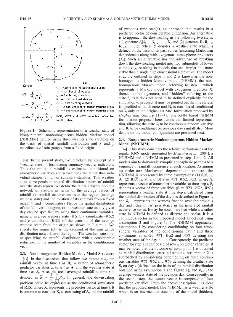
[14] In the present study, we introduce the concept of a‘weather state’ in formulating summary weather indicators.Thus the multisite rainfall is estimated conditional onatmospheric variables and a weather state rather than indi-vidual station rainfall or summary statistics. This weatherstate corresponds to spatial distribution pattern of rainfallover the study region. We define the rainfall distribution at anetwork of stations in terms of the average values ofrainfall or rainfall occurrences over the region (averagewetness state) and the location of its centroid from a fixedorigin (x and y coordinates). Hence the spatial distributionof rainfall over the region, or the weather state on any givenday can be specified by using three continuous variables,namely, average wetness state (WS1), x coordinate (WS2)and y coordinate (WS3) of the centroid of the averagewetness state from the origin as shown in Figure 1. Wespecify the origin (O) as the centroid of the rain gaugedistribution network over the region. The weather state aimsat specifying the rainfall distribution with a considerablereduction in the number of variables in the conditioningvector.

2.3. Nonhomogenous Hidden Markov Model Structure

[15] In the discussions that follow, we denote a ns-siterainfall vector at time t as Rt, a vector of atmosphericpredictor variables at time t as At and the weather state attime t as St. Also, the areal averaged rainfall at time t is

denoted as Rt =1

ns

Pnsi¼1

Ri,t. In general, the downscaling

problem could be expressed as the conditional simulationof RtjXt where Xt represents the predictor vector at time t. Itis common to consider Xt as consisting of At and the rainfall

of previous time step(s), an approach that results in apredictor vector of considerable dimension. An alternativeis to approach the downscaling in the following two steps:(1) generate StjSt�1, St�2, . . ., Xt and (2) generate RtjRt�1,Rt�2, . . ., St, where St denotes a weather state which isdefined on the basis of its past values (assuming Markoviandependence) along with exogenous atmospheric predictors(Xt). Such an alternative has the advantage of breakingdown the downscaling model into two submodels of lowercomplexity, resulting in models that are simpler and morestable than a single high-dimensional alternative. The modelstructure outlined in steps 1 and 2 is known as the non-homogenous hidden Markov model (NHMM), the non-homogenous Markov model referring to step 1 whichrepresents a Markov model with exogenous predictor Xt

(hence nonhomogenous), and ‘‘hidden’’ referring to thestate St as it does not need to be defined explicitly for thesimulation to proceed. It must be pointed out that the state Stis specified to be discrete and Rt is considered conditionalon St only in the original NHMM formulation proposed byHughes and Guttorp [1994]. The KNN based NHMMformulation proposed here avoids this limited representa-tion, allowing the state St to be continuous random variableand Rt to be conditional on previous day rainfall also. Moredetails on the model configuration are presented next.

2.4. Nonparametric Nonhomogeneous Hidden MarkovModel (NNHMM)

[16] This study considers the relative performances of theregular KNN model presented by Mehrotra et al. [2004], aNNHMM and a NHMM as presented in steps 1 and 2. Allmodels aim to downscale synoptic atmospheric patterns to asequence of rainfall occurrence at each location. Assumingan order-one Markovian dependence structure, theNNHMM is represented by three assumptions: (1) StjSt�1,At, (2) RtjRt�1, St, and (3) S � WS1, WS2, WS3, where At

represents a vector of atmospheric variables at time step t, Stdenotes a vector of three variables (S � WS1, WS2, WS3)representing a weather state at time step t, calculated usingthe rainfall distribution of the day t as described in Figure 1,and Rt�1 represents the wetness fraction over the previousday and helps impart persistence in the generated rainfalloccurrence series. It may be noted here that while a weatherstate in NHMM is defined as discrete and scalar, it is acontinuous vector in the proposed model as defined usingassumption 3 and Figure 1. The NNHMM approachesassumption 1 by considering conditioning on four atmo-spheric variables of the conditioning day t and threecontinuous variables WS1, WS2 and WS3 defining theweather state of the day t � 1. Consequently, the predictorvector for step 1 is composed of seven predictor variables. Itmay be noted that the outcome of assumption 1 is obtainedas rainfall distribution across all stations. Assumption 2 isapproached by considering conditioning on three continu-ous variables WS1, WS2 and WS3 defining the weather stateSt on day t (defined on the basis of the rainfall distributionobtained using assumption 1 and Figure 1), and Rt�1, theaverage wetness state of the previous day. Consequently, inthe second step, the feature vector is composed of fourpredictor variables. From the above description it is clearthat the proposed model, like NHMM, has a weather statewhich is an intermediate outcome of the model (hidden),

Figure 1. Schematic representation of a weather state ofNonparametric nonhomogeneous hidden Markov model(NNHMM) defined using three weather state variables onthe basis of spatial rainfall distribution and x and ycoordinates of rain gauges from a fixed origin.

D16108 MEHROTRA AND SHARMA: A NONPARAMETRIC NHMM MODEL

4 of 13

D16108

however, is continuous in nature. As the weather state isrepresented as a vector (assumption 3), it is desirable toobtain the outcome of assumption 1 as rainfall distributionat stations and thereafter use this distribution to define theweather state vector on the day t (using assumption 3 andFigure 1).[17] The second model (KNN) is a traditional KNN

model in which the feature vector of equation (1a)consists of four atmospheric variables of the conditioningday (day t) and the average wetness state of the previousday (day t � 1) (Rt�1). Note that both KNN formulationsevaluated here use a moving window of length l (seeMehrotra et al., 2004 for details and rationale) as thebasis for representing smooth seasonal variations acrossthe simulations.[18] The third and final model is a six-state NHMM.

NHMM structure and parameterization are discussed indetail by Hughes and Guttorp [1994] and Mehrotra et al.[2004]. The optimal model structure of NHMM wasinvestigated thoroughly using the same data set given byMehrotra et al. [2004]. Readers are referred to Mehrotra etal. [2004] for the rationale behind the specific modelconfiguration presented here.

2.5. Estimation of Parameters of the DownscalingModels Used in the Study

[19] Apart from finalizing the predictors to be included inthe feature vector, the scaling weight vector S, the numberof nearest neighbor k, the length of the moving window ‘,and the influence weight vector B form the parameters ofboth KNN downscaling approaches.2.5.1. Selection of Scaling Weight Vector s[20] Predictor variables used in the calculation of

Euclidean distances are made dimensionless throughstandardization using scaling weights. Scaling of variablesalso reduces the effects of seasonal variation. Scaling isalso necessary when the feature vector consists of combi-nation of discrete and continuous variables [Sharma andLall, 1999; Buishand and Brandsma, 2001]. The reciprocalof the standard deviation of each variable in the predictorset is a common choice for the scaling weights [Lall andSharma, 1996; Rajagopalan and Lall, 1999; Sharma andLall, 1999; Harrold et al., 2003a; Beersma and Buishand,2003].2.5.2. Selection of Number of Nearest Neighbors K[21] The choice of K depends on the nature of the

conditional distribution or kernel, the total number ofobservations, N, from which the nearest neighbors areselected, and the dimension, m, of the predictor vector.Also, the optimal K value differs when used in the contextof time series simulation as compared to when used forprediction [see, e.g., Buishand and Brandsma, 2001]. Ingeneral, the optimal K will be smaller when the purpose istime series simulation than when the purpose is prediction.However, a small number of nearest neighbors may havethe danger of duplicating the large part of the historicrecord in the simulated series. Lall and Sharma [1996]recommended that for the KNN kernel (equation (2)) withsmaller number of predictor variables (m < 6), thenumber of nearest neighbors K can be considered equalto the square root of the number of observations. Fortime series simulation, Buishand and Brandsma [2001]

found better results with small K (�5). Mehrotra andSharma (unpublished manuscript, 2005) recommendedestimating the number of nearest neighbors based on aleave-one-out cross-validation (L1CV) optimizationprocedure. For both KNN formulations, based on theresults of a sensitivity analysis to the optimal value ofK, the number of nearest neighbors, a value of K = 7, isadopted for use in the present study.2.5.3. Estimation of Optimal Values of InfluenceWeights B[22] The influence weights B aim to define the relative

influence each predictor variable has on the conditionalPDF. The appropriate set of values for the influence vectorB is ascertained by minimizing the predictive error associ-ated with the model as assessed using L1CV and isascertained again on the basis of an optimization procedure,as described by Mehrotra and Sharma (unpublished manu-script, 2005). This measure of the predictive error is used tospecify the log likelihood associated with the B. The optimalvalues of the influence weights B for both KNN models areestimated by using an adaptive Metropolis (AM) samplingapproach [Haario et al., 2001; Marshall et al., 2004]. Thisapproach is based on the maximization of log likelihood forbinary data:

l RjQð Þ ¼Xnsi¼1

XNt¼1

log Pt;i

� �Rt;i þ log 1� Pt;i

� �� �1� Rt;i

� �� �ð6Þ

where l(RjQ) is the log likelihood, Rt,i is the observedrainfall occurrence at the ith station at time t (a value of 0or 1) and Pt,i is the modeled probability of occurrence of therainfall (Pt,i = P[Rt,i = 1], Rt,I here referring to the randomvariable representing the rainfall occurrence state at time t,station i.). Further, ns defines the number of stations theatmospheric predictors are being downscaled to, N is totalnumber of observations in the moving window and Q is theset of model parameters.[23] The probability of occurrence of the observed rain-

fall, Pt,i, is estimated as

Pt;i ¼ P Rt;i ¼ 1j Xt; Qð Þ� �

¼ P StjðSt�1;Xt; Q½ � P Rt;i ¼ 1jSt ;Rt�1; Q� �

¼Xl

p Slð ÞXk

p Rk;i ¼ 1jSl� �" #

ð7Þ

where p(Sl) denotes the probability of sampling state Sl,estimated as the KNN probability in (4) and p(Rk,i = 1) is theprobability of sampling rainfall occurrence Rk,I as wet,conditional to the sample state Sl, estimated again as theKNN probability in (4) but set equal to zero when Rk,i = 0.Rt�1 is the average wetness fraction of the previous day.The adaptive Metropolis (AM) algorithm [Haario et al.,2001; Marshall et al., 2004] is characterized by aproposal distribution based on the estimated posteriorcovariance matrix of the parameters. At step t, Haario etal. [2001] consider a multivariate normal proposal withmean given by the current value, N(Qt, Ct) where Ct isthe proposal covariance. The covariance Ct has a fixed

D16108 MEHROTRA AND SHARMA: A NONPARAMETRIC NHMM MODEL

5 of 13

D16108

value (C0) for the first few iterations and is updated aftera t0 iterations as

Ct ¼C0 t � t0

hCov Q0; � � � ; Qt�1ð Þ þ heId t > t0

�ð8Þ

where e is a parameter chosen to ensure Ct does notbecome singular; and h is a scaling parameter to ensurereasonable acceptance rates of the proposed states. Thesteps involved in our implementation of the AMalgorithm are as follows:[24] 1. Initialize t = 0 and set C0 as a diagonal matrix with

each diagonal term representing the variance associatedwith the prior distribution for each unknown.[25] 2. Update Ct for the current iteration number t using

equation (8).[26] 3. Generate a proposed value Q* for Q, where Q*

N(Qt, Ct). If parameter values are outside the parameterconstraints, repeat the step again. The constraints for the B

parameters are defined as

Xm

j¼1�j ¼ 1:0; and 0 < �j < 1:0 ð9Þ

These conditions ensure that the relative magnitude of eachparameter is retained and it remains bounded.[27] 4. Compute the log likelihood p(RjQ*) using (6)

using the L1CV procedure.[28] 5. Calculate the acceptance probability, a, of the

proposed parameter values using

a ¼ min 1; exp p RjQ*ð Þ þ p Q*ð Þ � p RjQtð Þ � p Qtð Þ½ f g ð10Þ

where p(Q) is the log prior distribution of Q, the priors beingspecified as a Uniform PDF over [0,1] for each element ofthe influence weight vector B.[29] 6. Generate u U[0,1]. If u < a, accept Qt+1 = Q*,

otherwise set Qt+1 = Qt. Repeat steps 2–6 a sufficientnumber of times to ensure that the posterior distributionof the parameter vector q has been sampled exhaustively.[30] The scaling weights h and the stopping criterion for

our algorithm are based on the recommendations ofMarshall et al. [2004] and Haario et al. [2001]. Many runswith different initial values of model parameters Q arecarried out to determine the reasonable values of initialset of parameters. As a guide line, in the beginning, B

parameters may be assigned equal values in line withequation (9). We found final convergence to be very slow.However, as many runs with different initial values ofparameters are carried out, we are confident of attainingthe optimum solution. Out of these runs, optimized sets ofparameter values for each formulation are selected on thebasis of maximized likelihood score. Standard convergencetests [Marshall et al., 2004] are used to assess the adequacyof the number of iterations in each application.2.5.4. Selection of Width of Moving Window[31] To account far the seasonality in hydrologic record,

Rajagopalan and Lall [1999] and Sharma and Lall [1999]suggested to use a moving window of length ‘ days,centered on the current day and estimate the conditionalprobability density based on the samples included withinthis moving window. For both KNN formulations, on the

basis of the results of a sensitivity analysis to differentchoices of width of moving window ‘, a value of ‘ = 15 daysis chosen for use in our study.

2.6. Adjustment of Bias in the Wet Day Probabilities atAll Stations

[32] Mehrotra et al. [2004] observed that the KNNmultisite downscaling model used by them under estimatedthe wet day probabilities at all stations. The optimizationprocedure used here provides an additional advantage ofavoiding this bias by penalizing the log likelihood ofequation (6). This penalty is imposed by modifying thelog likelihood using a Lagrangian multiplier (l) and the rootmean square difference (e) of observed and predicted wetday probabilities at all stations:

e ¼

ffiffiffiffiffiffiffiffiffiffiffiffiffiffiffiffiffiffiffiffiffiffiffiffiffiffiffiffiffiffiffiffiffiffiffiffiffiffiXns

j¼1

phj � pgj� �2

ns

sð11Þ

l0 RjQð Þ ¼ l RjQð Þ þ el ð12Þ

where l0(RjQ) is the modified log likelihood, phj and pgj areobserved and estimated wet day probabilities at the jthstation, and ns is total number of stations. The appropriatevalue of Lagrangian multiplier (l) is selected based on theaverage value of the bias and the log likelihood. For thecurrent application l is adopted as 20 times the averagevalue of original log likelihood. This arrangement helped ingetting the final optimized parameter values that producedunbiased wet day probabilities without much loss ofinformation at other levels. It may be mentioned here thatmodifying the likelihood using a penalty function mightaffect adversely some of the statistics of the simulatedseries. Therefore care should be taken while applying suchpenalties by verifying various statistics of the simulatedseries.[33] It may be noted that for weather state resampler,

WS1, WS2 and WS3 variables define the weather state ofprevious day in assumption 1, while these represent theweather state of the current day in assumption 2. However,in the present study, the influence weights associated withthese variables do not vary with the assumptions. Consid-ering the Markovian assumption of the weather states, thisassumption would not affect the model results.[34] Parameters of NHMM were obtained using the

similar sampling approach as used for estimation of optimalvalues of influence weights B and described in section 2.5.3,however, with different likelihood measure. The NHMMused was a six-state model having the same four atmo-spheric predictors as used in the NNHMM. Readers arereferred to Mehrotra et al. [2004] for details of the param-eter estimation procedure adopted for the model.

3. Model Application and Comparison of Results

[35] This section presents the details on the data and thestudy region used, the application of the various modelsconsidered, and their result comparison.

3.1. Data and Study Area

[36] The study region is located around Sydney, easternAustralia, spanning between 147�E–153�E longitude and

D16108 MEHROTRA AND SHARMA: A NONPARAMETRIC NHMM MODEL

6 of 13

D16108

31�S–36�S latitude (Figure 2). The most significant rainfallevents in winter in this region involve air masses that havebeen brought over the region from the east coast low-pressure systems. Orographic uplift of these air masseswhen they strike coastal ranges or the Great Dividing Rangeoften produces very heavy rain. For this study, a 43-yearcontinuous record (from 1960 to 2002) of daily winterrainfall occurrences at 30 stations around Sydney, easternAustralia (see Figure 2), was used. The interstation dis-tances between station pairs vary approximately from 20 to340 km. Six winter months from March to August(184 days) were pooled together for the analysis. Missingvalues at some stations (<0.5%), were estimated usinginverse distance averaging and the records of nearbystations. A day was considered as a wet day or dry daydepending on whether the rainfall amount was greaterthan or equal to, or less than 0.3 mm respectively [afterBuishand, 1978; Harrold et al., 2003a, 2003b; Mehrotra etal., 2004].[37] The study uses four atmospheric predictor variables

that signify the state of the atmosphere in predicting therainfall pattern on ground for this region. Mehrotra et al.[2004] identified mean sea level pressure (MSLP), east-westgradient of MSLP and the north-south gradient of geo-potential heights (GPH) at 700 hPa as the significantatmospheric predictors for modeling precipitation occur-rence at multiple rain gauge stations using the NHMMand the KNN model. Further consultations with climatolo-gists and hydrologists indicated that total precipitable watercontent may also have a strong influence in driving rainfallmechanism over the region. Consequently, total precipitablewater content was also included as an additional predictorvariable in our analysis. If any of these variables are notsignificant, our optimization technique should take care ofthat by assigning negligible weight to them.[38] The required atmospheric data was extracted from

the National Center for Environmental Prediction (NCEP)reanalysis data provided by the NOAA-CIRES ClimateDiagnostics Center, Boulder, Colorado, USA, from theirweb site at http://www.cdc.noaa.gov/. These variables wereavailable on 2.5� latitude � 2.5� longitude grid over thestudy region, 4 times a day for the same period as the

rainfall record and were estimated over 5 � 5 (total of 25)grid nodes. As an observed rainfall value represents thetotal rainfall over a 24-hour period ending at 0900 LT inthe morning, the available atmospheric measurements at1700 LT on the preceding day were considered as represen-tative of today’s rainfall.

3.2. Model Results

[39] For a fair comparison of these models, model resultspresented next are evaluated using a leave-6-year-out crossvalidation. Leave-6-year-out cross validation (L6YCV) is aspecific case of cross validation where the model is formu-lated using all observations except 6 years, and predictionerror assessed by applying the model on the observationperiod that has been left out. For the present study, L6YCVwas performed by dividing the complete record of 43 yearsinto blocks of 6 years (the last block being 7 years long),and estimating the rainfall for each block one at a time withthe model being formulated using the remaining data[Mehrotra et al., 2004]. The choice of 6 years for the crossvalidation was based on having a long enough period ofcross validation for estimation of relevant persistence char-acteristics (such as maximum spell lengths). Significantdifferences were not observed in any of the results reportedbelow in the statistics estimated for each of the 6-year cross-validation periods (suggesting that all models wererelatively stable in their performance over each 6-yearsegment). In all the approaches, results were ascertainedby generating 100 realizations of the rainfall occurrences,on the basis of which statistical performance measureswere estimated. The comparison of results was based onthe reproduction of various statistics of interest, represent-ing spatial and temporal characteristics of rainfall includ-ing those of importance to water resources planning andmanagement.[40] The graphical comparison of different models was

performed on the basis of: (1) log-odds ratio, a measure ofthe spatial correlation in the rainfall occurrence; (2) seasonalwetness state, a measure of the frequency at which wet daysare predicted within the season; (3) weather state wetnessstate, a measure of the frequency at which wet days arepredicted within each discrete weather state; (4) successrates of wet and dry days, a measure of the similarity (wet/dry) in the observed and predicted rainfall occurrences on agiven day; and (5) maximum wet and dry spells, a measureof longer time dependence in the simulated rainfall series.Numerical comparisons were based on the estimation of theroot mean square error (RMSE) for the above statistics andother statistics of interest.3.2.1. Spatial Dependence[41] The log-odds ratio, reflecting the spatial correlation

between rainfall occurrences at each pair of stations pro-vides a measure of accurate reproduction of the spatialdependence of long spells of rainfall events [Mehrotra etal., 2004]. Figure 3 presents observed and modeled log-odds ratios for KNN models and NHMM at all stations.Each point on the graph indicates the ratio evaluated for apair of rain gauge stations. As KNN approach considersprecipitation occurrences concurrently at all the stations, thedependence between the stations is automatically preservedby both KNN formulations. The NHMM which aims toexplain the spatial correlation in the form of a common

Figure 2. Map of the study area showing the locations ofrain gauge stations and atmospheric data grid.

D16108 MEHROTRA AND SHARMA: A NONPARAMETRIC NHMM MODEL

7 of 13

D16108

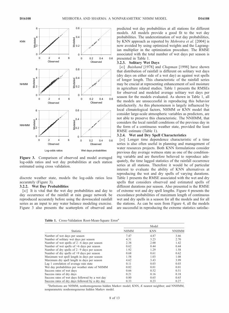
discrete weather state, models the log-odds ratios lessaccurately (Figure 3).3.2.2. Wet Day Probabilities[42] It is vital that the wet day probabilities and day to

day occurrence of the rainfall at rain gauge network bereproduced accurately before using the downscaled rainfallseries as an input to any water balance modeling exercise.Figure 3 also presents the scatterplots of observed and

predicted wet day probabilities at all stations for differentmodels. All models provide a good fit to the wet dayprobabilities. The underestimation of wet day probabilities,by KNN approach as reported by Mehrotra et al. [2004] isnow avoided by using optimized weights and the Lagrang-ian multiplier in the optimization procedure. The RMSEassociated with the total number of wet days per season ispresented in Table 1.3.2.3. Solitary Wet Days[43] Buishand [1978] and Chapman [1998] have shown

that distribution of rainfall is different on solitary wet days(dry days on either side of a wet day) as against wet spellsof longer length. This characteristic of the rainfall seriesmay be crucial at representing enhancement of soil moisturein agriculture related studies. Table 1 presents the RMSEsfor observed and modeled average solitary wet days perseason for the models evaluated. As shown in Table 1, allthe models are unsuccessful in reproducing this behaviorsatisfactorily. As this phenomenon is largely influenced bylocal climatological factors, NHMM or KNN model thatconsider large-scale atmospheric variables as predictors, arenot able to preserve this characteristic. The NNHMM, thatconsiders the local rainfall conditions of the previous day inthe form of a continuous weather state, provided the leastRMSE estimate (Table 1).3.2.4. Wet and Dry Spell Characteristics[44] Longer time dependence characteristic of a time

series is also often useful in planning and management ofwater resources projects. Both KNN formulations considerprevious day average wetness state as one of the condition-ing variable and are therefore believed to reproduce ade-quately, the time lagged statistics of the rainfall occurrenceseries at all stations. Therefore it would be of particularinterest to evaluate the ability of KNN alternatives atreproducing the wet and dry spells of varying durations.Table 1 presents the RMSE associated with the wet and dryspells that considers observed and estimated spells ofdifferent durations per season. Also presented is the RMSEof extreme wet and dry spell lengths. Figure 4 presents theexceedance probabilities of maximum length of continuouswet and dry spells in a season for all the models and for allthe stations. As can be seen from Figure 4, all the modelsare successful in reproducing the extreme statistics satisfac-

Figure 3. Comparison of observed and model averagedlog-odds ratios and wet day probabilities at each stationestimated using cross validation.

Table 1. Cross-Validation Root-Mean-Square Errora

Statistic

Model

NHMM KNN NNHMM

Number of wet days per season 7.47 4.87 3.66Number of solitary wet days per season 4.31 3.23 2.70Number of wet spells of 2–6 days per season 2.38 2.00 1.42Number of wet spells of >6 days per season 0.62 0.44 0.44Number of dry spells of 2–9 days per season 1.92 1.29 1.58Number of dry spells of >9 days per season 0.68 0.61 0.62Maximum wet spell length in days per season 1.58 1.03 1.08Maximum dry spell length in days per season 4.62 3.43 3.99Lag 1 correlation of average rain state 0.11 0.03 0.03Wet day probabilities per weather state of NHMM 0.02 0.01 0.01Success rates of wet days 0.66 0.52 0.51Success rates of dry days 0.21 0.16 0.18Success rates of wet days followed by a wet day 0.80 0.65 0.65Success rates of dry days followed by a dry day 0.33 0.23 0.27

aDefinitions are NHMM, nonhomogeneous hidden Markov model; KNN, K nearest neighbor; and NNHMM,nonparametric nonhomogeneous hidden Markov model.

D16108 MEHROTRA AND SHARMA: A NONPARAMETRIC NHMM MODEL

8 of 13

D16108

torily. However, NNHMM and KNN are more successful inreproducing these statistics in comparison to NHMM. Plotsof wet and dry spells durations also conveying similarresults are not presented here.3.2.5. Wet Day Probabilities for NHMM DiscreteWeather States[45] A discrete weather state classification can be used to

classify the days under a particular weather state. It wouldbe of interest to evaluate the performance of models on thebasis of number of wet days predicted under a particularweather state at a station. For a fair comparison of themodels used in the study, we adopted the weather stateclassification criterion of NHMM for comparison of allmodels including KNN and NNHMM. Each day of thehistorical record is assigned a discrete weather state usingthe classification of NHMM. Averaging of all wet days at astation falling under a particular weather state provided theobserved wet day probability for that particular weatherstate at that station. Using the same historical weather stateassignment for a given day, repetition of same exercise onpredicted results of NHMM, KNN and NNHMM providedpredicted wet day probabilities for each weather state ateach station. The RMSE associated with the wet dayprobabilities per weather state of NHMM per station ispresented in Table 1. Figure 5 presents the scatterplots of

observed and predicted wet day probabilities by all themodels for three weather states of NHMM. Each point onthe graph represents the wet day probability at a stationunder the given weather state. As can be seen from Figure 5and Table 1, all models are unsuccessful in reproducingadequately, the high wet day probabilities. However,NNHMM and KNN models reproduce this statistic muchbetter in comparison to NHMM.3.2.6. Success Rates of Wet and Dry Days[46] The sequencing of wet and dry days defines the day

to day persistence of the daily rainfall and help in represent-ing the wet and dry spells of longer durations. Suchrepresentation of wet and dry days similar to what has beenobserved is of prime concern in catchment managementstudies. The success rate is defined as the ratio of number ofdays when both observed and predicted values are wet (dry)to the total number of wet (dry) days in the observed record.In case of perfect match the success rate approaches unity.Figure 6 presents the success rates of wet and dry days ateach station predicted by all models. The associated RMSEsare presented in Table 1. As can be seen from Figure 6, allthe models under estimate the success rates of wet anddry days. However, NNHMM and KNN are more success-

Figure 4. Comparison of observed and model-averagedexceedance probabilities of maximum wet and dry spelllengths per season at each station estimated using crossvalidation.

Figure 5. Comparison of observed and model averagedwet day probabilities under a weather state of nonhomoge-neous hidden Markov model (NHMM), per season, at eachstation, for NHMM (six states), K nearest neighbor (KNN),and NNHMM estimated using cross validation (resultsshown for weather states 1, 3, and 4 only).

D16108 MEHROTRA AND SHARMA: A NONPARAMETRIC NHMM MODEL

9 of 13

D16108

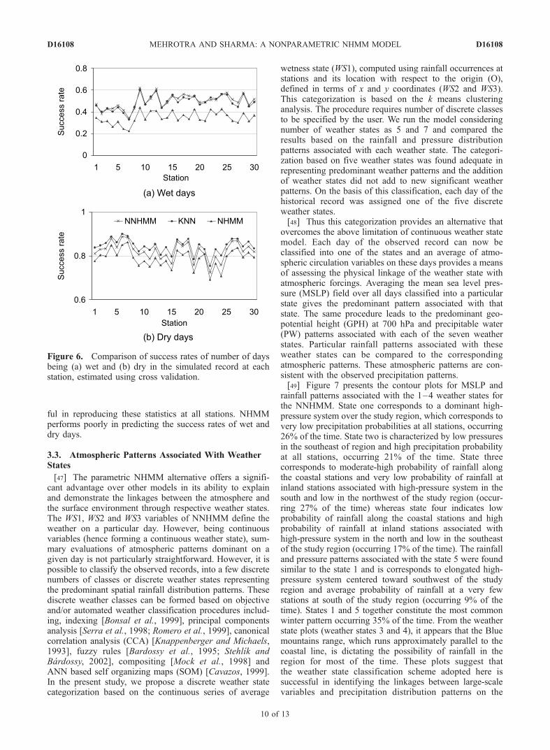
ful in reproducing these statistics at all stations. NHMMperforms poorly in predicting the success rates of wet anddry days.

3.3. Atmospheric Patterns Associated With WeatherStates

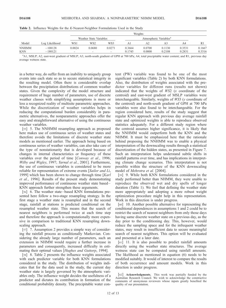
[47] The parametric NHMM alternative offers a signifi-cant advantage over other models in its ability to explainand demonstrate the linkages between the atmosphere andthe surface environment through respective weather states.The WS1, WS2 and WS3 variables of NNHMM define theweather on a particular day. However, being continuousvariables (hence forming a continuous weather state), sum-mary evaluations of atmospheric patterns dominant on agiven day is not particularly straightforward. However, it ispossible to classify the observed records, into a few discretenumbers of classes or discrete weather states representingthe predominant spatial rainfall distribution patterns. Thesediscrete weather classes can be formed based on objectiveand/or automated weather classification procedures includ-ing, indexing [Bonsal et al., 1999], principal componentsanalysis [Serra et al., 1998; Romero et al., 1999], canonicalcorrelation analysis (CCA) [Knappenberger and Michaels,1993], fuzzy rules [Bardossy et al., 1995; Stehlık andBardossy, 2002], compositing [Mock et al., 1998] andANN based self organizing maps (SOM) [Cavazos, 1999].In the present study, we propose a discrete weather statecategorization based on the continuous series of average

wetness state (WS1), computed using rainfall occurrences atstations and its location with respect to the origin (O),defined in terms of x and y coordinates (WS2 and WS3).This categorization is based on the k means clusteringanalysis. The procedure requires number of discrete classesto be specified by the user. We run the model consideringnumber of weather states as 5 and 7 and compared theresults based on the rainfall and pressure distributionpatterns associated with each weather state. The categori-zation based on five weather states was found adequate inrepresenting predominant weather patterns and the additionof weather states did not add to new significant weatherpatterns. On the basis of this classification, each day of thehistorical record was assigned one of the five discreteweather states.[48] Thus this categorization provides an alternative that

overcomes the above limitation of continuous weather statemodel. Each day of the observed record can now beclassified into one of the states and an average of atmo-spheric circulation variables on these days provides a meansof assessing the physical linkage of the weather state withatmospheric forcings. Averaging the mean sea level pres-sure (MSLP) field over all days classified into a particularstate gives the predominant pattern associated with thatstate. The same procedure leads to the predominant geo-potential height (GPH) at 700 hPa and precipitable water(PW) patterns associated with each of the seven weatherstates. Particular rainfall patterns associated with theseweather states can be compared to the correspondingatmospheric patterns. These atmospheric patterns are con-sistent with the observed precipitation patterns.[49] Figure 7 presents the contour plots for MSLP and

rainfall patterns associated with the 1–4 weather states forthe NNHMM. State one corresponds to a dominant high-pressure system over the study region, which corresponds tovery low precipitation probabilities at all stations, occurring26% of the time. State two is characterized by low pressuresin the southeast of region and high precipitation probabilityat all stations, occurring 21% of the time. State threecorresponds to moderate-high probability of rainfall alongthe coastal stations and very low probability of rainfall atinland stations associated with high-pressure system in thesouth and low in the northwest of the study region (occur-ring 27% of the time) whereas state four indicates lowprobability of rainfall along the coastal stations and highprobability of rainfall at inland stations associated withhigh-pressure system in the north and low in the southeastof the study region (occurring 17% of the time). The rainfalland pressure patterns associated with the state 5 were foundsimilar to the state 1 and is corresponds to elongated high-pressure system centered toward southwest of the studyregion and average probability of rainfall at a very fewstations at south of the study region (occurring 9% of thetime). States 1 and 5 together constitute the most commonwinter pattern occurring 35% of the time. From the weatherstate plots (weather states 3 and 4), it appears that the Bluemountains range, which runs approximately parallel to thecoastal line, is dictating the possibility of rainfall in theregion for most of the time. These plots suggest thatthe weather state classification scheme adopted here issuccessful in identifying the linkages between large-scalevariables and precipitation distribution patterns on the

Figure 6. Comparison of success rates of number of daysbeing (a) wet and (b) dry in the simulated record at eachstation, estimated using cross validation.

D16108 MEHROTRA AND SHARMA: A NONPARAMETRIC NHMM MODEL

10 of 13

D16108

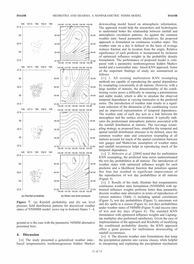
ground as is the case with the parametric NHMM alternativepresented here.

4. Discussion

[50] The study presented a generalized weather state–based nonparametric nonhomogeneous hidden Markov

downscaling model based on atmospheric information.The approach would help the researchers and hydrologiststo understand better the relationship between rainfall andatmospheric circulation patterns. As against the commonweather state–based parametric alternatives, the proposedapproach is formulated on continuous weather states. Theweather state on a day is defined on the basis of averagewetness fraction and its location from the origin. Relativesignificance of each predictor is incorporated by inclusionof optimized influence weights in the probability densityformulation. The performance of proposed model is com-pared with a parametric nonhomogenous hidden Markovmodel and a nonweather state–based KNN approach. Someof the important findings of study are summarized asfollows:[51] 1. All existing multistation KNN resampling

methods are capable of reproducing the spatial dependenceby resampling concurrently at all stations. However, with alarge number of stations, the dimensionality of the condi-tioning vector poses a difficulty in ensuring a parsimoniousand stable model, which is able to simulate the observedtemporal dependence at varying timescales in the predictedseries. The introduction of weather state results in a signif-icant reduction of the dimension of the conditioning vectorand an improved representation of temporal dependence.The weather state of each day acts as a link between theatmosphere and the surface environment. It typically indi-cates the predominant atmospheric patterns associated withthe rainfall distribution at stations. The two-stage resam-pling strategy as proposed here, simplifies the temporal andspatial rainfall distribution structure to be defined, since thecommon weather state and concurrent resampling at allstations account for much of the spatial correlation betweenrain gauges and Markovian assumption of weather statesand rainfall occurrences helps in reproducing much of thetemporal dependence.[52] 2. Mehrotra et al. [2004] noted that for multistation

KNN resampling, the predicted time series underestimatedthe wet day probabilities at all stations. The introduction ofweather states with optimized influence weight for eachpredictor and a likelihood function that penalizes againstthis bias has resulted in significant improvement ofthe reproduction of wet day probabilities at all stations(Figure 3).[53] 3. Results of the study illustrate that nonparametric

continuous weather state formulation (NNHMM) with op-timized influence weights performs better than parametricdiscrete weather state alternative in terms of reproduction ofvarious statistics (Table 1) including spatial correlations(Figure 3), wet day probabilities (Figure 3), maximum wetand dry spells in a season (Figure 4), wet days probabilitiesunder weather states of NHMM (Figure 5) and success ratesof wet and dry days (Figure 6). The standard KNNformulation with optimized influence weights and Lagrang-ian multiplier also performed satisfactory. Given the ease ofimplementation of the approach and flexibility of modifyingthe conditional probability density, the KNN approachoffers a great promise for multistation downscaling ofrainfall occurrences.[54] 4. The discrete weather state formulations that lump

the precipitation patterns into various classes, while helpfulin interpreting and explaining the precipitation mechanism

Figure 7. (a) Rainfall probability and (b) sea levelpressure field distribution patterns for discretized weatherstates of NNHMM model. (rows top to bottom) States 1–4.

D16108 MEHROTRA AND SHARMA: A NONPARAMETRIC NHMM MODEL

11 of 13

D16108

in a better way, do suffer from an inability to uniquely groupevents into each state so as to secure statistical integrity inthe resulting model. Often there is considerable overlapbetween the precipitation distributions of common weatherstates. Given the complexity of the model structure andrequirement of huge number of parameters, use of discreteweather classes with simplifying assumptions is more orless a recognized reality of multisite parametric approaches.While the discretization of weather variables helps inreducing the computational burden considerably in para-metric alternatives, the nonparametric approaches offer theeasy and straightforward alternative of using the continuousweather variables.[55] 5. The NNHMM resampling approach as proposed

here makes use of continuous series of weather states andtherefore avoids the limitations of discrete weather statemodels as mentioned earlier. The approach being based oncontinuous series of weather variables, can also take care ofthe type of nonstationarity that is developed because ofchanges in internal characteristics or frequency of thesevariables over the period of time [Conway et al., 1996;Wilby and Wigley, 1997; Yarnal et al., 2001]. Furthermore,the use of continuous variables is considered to be morereliable for representation of extreme events [Sailor and Li,1999] which has been shown to change through time [Karlet al., 1996]. Results of the present study demonstratingimproved performance of continuous weather state based–KNN approach further strengthen these arguments.[56] 6. The weather state–based KNN formulations pre-

sented here follow a two-stage resampling strategy. In thefirst stage a weather state is resampled and in the secondstage, rainfall at stations is predicted conditional on theresampled weather state. This means that the search ofnearest neighbors is performed twice at each time stepand therefore the approach is computationally more expen-sive in comparison to traditional KNN resampling down-scaling approach.[57] 7. Assumption 2 provides a simple way of consider-

ing the rainfall process as conditionally Markovian. Con-sidering the already large number of parameters, such anextension in NHMM would require a further increase inparameters and consequently, increased difficulty in esti-mating their optimal values [Hughes and Guttorp, 1994].[58] 8. Table 2 presents the influence weights associated

with each predictor variable for both KNN formulationsconsidered in the study. The distribution of weights indi-cates that for the data used in the study, the current dayweather state is largely governed by the atmospheric vari-ables only. The influence weight decides the usefulness of apredictor and dictates its contribution in formation of theconditional probability density. The precipitable water con-

tent (PW) variable was found to be one of the mostsignificant variables (Table 2) by both KNN formulations.Also, the distribution of weights associated with the pre-dictor variables for different runs (results not shown)indicated that the weights of WS2 (x coordinate of thecentroid) and east-west gradient of MSLP variables wereinterchangeable. Similarly, weights of WS3 (y coordinate ofthe centroid) and north-south gradient of GPH at 700 hPavariables were also found to be interchangeable. For theregion considered here, results of the study suggest thatregular KNN approach with previous day average rainfallstate and optimized weights is able to reproduce observedstatistics adequately. For a different study region wherethe centroid assumes higher significance, it is likely thatthe NNHMM would outperform both the KNN and theNHMM. It must be emphasized here that the rationalebehind proposing the NNHMM was to enable a physicalinterpretation of the downscaling results through a statisticaldiscretization of the hidden states, as presented in Figure 7.Such an interpretation helps understand subtle shifts inrainfall patterns over time, and has implications in interpret-ing climate change scenarios. This interpretation is notpossible within the structure of the KNN downscalingmodel of Mehrotra et al. [2004].[59] 9. While both KNN formulations considered in the

study performed better than NHMM, they were unable toreproduce the observed wet and dry spells of longerduration (Table 1). We feel that defining the weather statemore appropriately and adopting a more robust weightoptimization procedure might help in this representation.Work in this direction is under progress.[60] 10. Another possible alternative for representing the

conditional dependences in assumptions 1 and 2 could be torestrict the search of nearest neighbors from only those dayshaving same discrete weather state on a previous day, as theday prior to the conditioning day. This, however, wouldreduce the sampling space and for the infrequent weatherstates, may result in insufficient data to secure meaningfulsearch of nearest neighbors. This option will be evaluatedand presented at a later date.[61] 11. It is also possible to predict rainfall amounts

directly using the weather state structures. The averagewetness state can be computed using rainfall amounts.The likelihood as mentioned in equation (6) needs to bemodified suitably. It would of interest to compare the resultsof both occurrence and amount models. Work in thisdirection is under progress.

[62] Acknowledgments. This work was partially funded by theAustralian Research Council. We wish to acknowledge the constructivecomments of anonymous reviewers whose inputs greatly benefited thequality of our presentation.

Table 2. Influence Weights for the K-Nearest-Neighbor Formulations Used in the Study

Model Log Likelihood

Weights

Weather State Variables Atmospheric Variablesa

R1WS1 WS2 WS3 A1 A2 A3 A4

NNHMM �108128 0.0024 0.0680 0.0271 0.3664 0.0700 0.1130 0.3531 0.1667KNN �180121 - - - 0.1745 0.0000 0.2108 0.2831 0.3316

aA1, MSLP; A2, east-west gradient of MSLP; A3, north-south gradient of GPH at 700 hPa; A4, total precipitable water content; and R1, previous dayaverage wetness state.

D16108 MEHROTRA AND SHARMA: A NONPARAMETRIC NHMM MODEL

12 of 13

D16108

ReferencesBardossy, A., and E. J. Plate (1992), Space-time models for daily rainfallusing atmospheric circulation patterns, Water. Resour. Res., 28, 1247–1259.

Bardossy, A., L. Duckstein, and I. Bogardi (1995), Fuzzy rule-basedclassification of atmospheric circulation patterns, Int. J. Climatol., 15,1087–1097.

Bates, B. C., S. P. Charles, and J. P. Hughes (1998), Stochastic downscalingof numerical climate model simulations, Environ. Modell. Software, 13,325–331.

Bates, B. C., S. P. Charles, and J. P. Hughes (2000), Stochastic downscalingof general circulation model simulations, in Applications of SeasonalClimate Forecasting in Agricultural and Natural Ecosystems: TheAustralian Experience, edited by C. J. Mitchell, pp. 121–134, Springer,New York.

Beersma, J. J., and T. A. Buishand (2003), Multi-site simulation of dailyprecipitation and temperature conditional on the atmospheric circulation,Clim. Res., 25, 121–133.

Bellone, E., J. P. Hughes, and P. Guttorp (2000), A hidden Markov modelfor downscaling synoptic atmospheric patterns to precipitation amounts,Clim. Res., 15, 1–12.

Bonsal, B. R., X. Zhang, and W. D. Hogg (1999), Canadian prairie growingseason precipitation variability and associated atmospheric circulation,Clim. Res., 11, 191–208.

Buishand, T. A. (1978), Some remarks on the use of daily rainfall models,J. Hydrol., 36, 295–308.

Buishand, T. A., and T. Brandsma (2001), Multisite simulation of dailyprecipitation and temperature in the Rhine basin by nearest-neighborresampling, Water Resour. Res., 37, 2761–2776.

Cavazos, T. (1999), Large-scale circulation anomalies conducive to extremeprecipitation events and derivation of daily rainfall in northeasternMexico and southeastern Texas, J. Clim., 12, 1506–1523.

Chapman, T. G. (1998), Stochastic modelling of daily rainfall: The impactof adjoining wet days on the distribution of rainfall amounts, Environ.Modell. Software, 13, 317–324.

Charles, S. P., B. C. Bates, and J. P. Hughes (1999), A spatiotemporalmodel for downscaling precipitation occurrence and amounts, J. Geo-phys. Res., 104(D24), 31,657–31,669.

Charles, S. P., B. C. Bates, and J. P. Hughes (2000), Statistical downscalingfrom numerical climate models for southwest Australia, paper presentedat Hydro 2000: 3rd International Hydrology and Water ResourcesSymposium, Inst. of Eng., Canberra, ACT.

Conway, D., R. L. Wilby, and P. D. Jones (1996), Precipitation and air flowindices over the British Isles, Clim. Res., 7, 169–183.

Efron, B., and R. Tibshirani (1993), An Introduction to the Bootstrap, CRCPress, Boca Raton, Fla.

Fowler, H. J., C. G. Kilsby, and P. E. O’Connell (2000), A stochasticrainfall model for the assessment of regional water resource systemsunder changed climatic conditions, Hydrol. Earth Syst. Sci., 4, 263–282.

Gyalistras, D., H. von Storch, A. Fischlin, and M. Beniston (1994), LinkingGCM-simulated climatic changes to ecosystem models: Case studies ofstatistical downscaling in the Alps, Clim. Res., 4, 167–189.

Haario, H., E. Saksman, and J. Tamminem (2001), An adaptive Metropolisalgorithm, Bernoulli, 7(2), 223–242.

Harrold, T. I., A. Sharma, and S. J. Sheather (2003a), A nonparametricmodel for stochastic generation of daily rainfall occurrence, WaterResour. Res., 39(12), 1300, doi:10.1029/2003WR002182.

Harrold, T. I., A. Sharma, and S. J. Sheather (2003b), A nonparametricmodel for stochastic generation of daily rainfall amounts, Water Resour.Res., 39(12), 1343, doi:10.1029/2003WR002570.

Hay, L., J. McCabe, D. M. Wolock, and M. A. Ayers (1991), Simulation ofprecipitation by weather type analysis, Water Resour. Res., 27, 493–501.

Hewitson, B. C., and R. G. Crane (1996), Climate downscaling: Techniquesand application, Clim. Res., 7, 85–95.

Hughes, J. P., and P. Guttorp (1994), A class of stochastic models forrelating synoptic atmospheric patterns to regional hydrologic phenomena,Water Resour. Res., 30, 1535–1546.

Hughes, J. P., P. Guttorp, and S. P. Charles (1999), A non-homogeneoushidden Markov model for precipitation occurrence, J. R. Stat. Soc. Ser. CAppl. Stat., 48(1), 15–30.

Karl, T. R., R. W. Knight, D. R. Easterling, and R. G. Quayle (1996),Indices of climate change for the United States, Bull. Am. Meteorol.Soc., 77, 279–292.

Knappenberger, P. C., and P. J. Michaels (1993), Cyclone tracks andwintertime climate in the mid-Atlantic region of the USA, Int. J. Clima-tol., 13, 509–531.

Lall, U., and A. Sharma (1996), A nearest neighbor bootstrap for time seriesresampling, Water. Resour. Res., 32, 679–693.

Marshall, L., D. Nott, and A. Sharma (2004), A comparative study ofMarkov chain Monte Carlo methods for conceptual rainfall-runoff model-ing,Water Resour. Res., 40, W02501, doi:10.1029/2003WR002378.

Mehrotra, R., A. Sharma, and I. Cordery (2004), Comparison of twoapproaches for downscaling synoptic atmospheric patterns to multisiteprecipitation occurrence, J. Geophys. Res., 109, D14107, doi:10.1029/2004JD004823.

Mock, C. J., P. J. Bartlein, and P. M. Anderson (1998), Atmosphericcirculation patterns and spatial climatic variations in Beringia, Int.J. Climatol., 18, 1085–1104.

Qian, B., J. Corte-Real, and H. Xu (2002), Multisite stochastic weathermodels for impact studies, Int. J. Climatol., 22, 1377–1397.

Rajagopalan, B., and U. Lall (1999), A k-nearest-neighbor simulator fordaily precipitation and other weather variables, Water Resour. Res., 35,3089–3101.

Romero, R., G. Summer, C. Ramis, and A. Genoves (1999), A classifica-tion of the atmospheric circulation patterns producing significant dailyrainfall in the Spanish Mediterranean area, Int. J. Climatol., 19, 765–785.

Sailor, D., and X. Li (1999), A semiempirical downscaling approach forpredicting regional temperature impacts associated with climate change,J. Clim., 12, 103–114.

Serra, C., G. Fernandez Mills, M. C. Periago, and X. Lana (1998), Surfacesynoptic circulation and daily precipitation in Catalonia, Theor. Appl.Climatol., 59, 29–49.

Sharma, A. (2000), Seasonal to interannual rainfall probabilistic forecastsfor improved water supply management: part 3—A nonparametric prob-abilistic forecast model, J. Hydrol., 239, 249–258.

Sharma, A., and U. Lall (1999), A nonparametric approach for daily rainfallsimulation, Math. Comput. Simul., 48, 361–371.

Sharma, A., and R. O’Neill (2002), A nonparametric approach for repre-senting interannual dependence in monthly streamflow sequences, WaterResour. Res., 38(7), 1100, doi:10.1029/2001WR000953.

Sharma, A., D. G. Tarboton, and U. Lall (1997), Streamflow simulation: Anonparametric approach, Water Resour. Res., 33, 291–308.

Souza Filho, F. A., and U. Lall (2003), Seasonal to interannual ensemblestreamflow forecasts for Ceara, Brazil: Applications of a multivariate,semiparametric algorithm, Water Resour. Res., 39(11), 1307,doi:10.1029/2002WR001373.

Stehlık, J., and A. Bardossy (2002), Multivariate stochastic downscalingmodel for generating daily precipitation series based on atmosphericcirculation, J. Hydrol., 256, 120–141.

Wilby, R. L. (1994), Stochastic weather type simulation for regional climatechange impact assessment, Water. Resour. Res., 30, 3395–3403.

Wilby, R. L. (1998), Statistical downscaling of daily precipitation usingdaily airflow and seasonal teleconnection indices, Clim. Res., 10, 163–178.

Wilby, R. L., and T. M. L. Wigley (1997), Downscaling general circulationmodel output: A review of methods and limitations, Prog. Phys. Geogr.,21, 530–548.

Wilks, D. S. (1999), Multisite downscaling of daily precipitation with astochastic weather generator, Clim. Res., 11, 125–136.

Wojcik, R., and T. A. Buishand (2003), Simulation of 6-hourly rainfall andtemperature by two resampling schemes, J. Hydrol., 273, 69–80.

Yakowitz, S. (1985), Nonparametric density estimation, prediction, andregression for Markov sequences, JASA J. Am. Stat. Assoc., 80(389),215–221.

Yarnal, B., A. C. Comrie, B. Frakes, and D. P. Brown (2001), Develop-ments and prospects in synoptic climatology, Int. J. Climatol., 21, 1923–1950.

Yates, D., S. Gangopaghyay, B. Rajagopalan, and K. Strzepek (2003), Atechnique for generating regional climate scenarios using a nearest-neighbor algorithm, Water Resour. Res., 39(7), 1199, doi:10.1029/2002WR001769.

Young, K. C. (1994), A multivariate chain model for simulating climaticparameters from daily data, J. Appl. Meteorol., 33, 661–671.

Zorita, E., and H. von Storch (1999), The analog method-A simplestatistical downscaling technique: Comparison with more complicatedmethods, J. Clim., 12, 2474–2489.

�����������������������R. Mehrotra and A. Sharma, School of Civil and Environmental

Engineering, University of New South Wales, Sydney, New South Wales,Australia. ([email protected])

D16108 MEHROTRA AND SHARMA: A NONPARAMETRIC NHMM MODEL

13 of 13

D16108