A non-linear 3D FEM model to simulate timber-concrete joints

This article was originally published in a journal published byElsevier, and the attached copy is provided by Elsevier for the

author’s benefit and for the benefit of the author’s institution, fornon-commercial research and educational use including without

limitation use in instruction at your institution, sending it to specificcolleagues that you know, and providing a copy to your institution’s

administrator.

All other uses, reproduction and distribution, including withoutlimitation commercial reprints, selling or licensing copies or access,

or posting on open internet sites, your personal or institution’swebsite or repository, are prohibited. For exceptions, permission

may be sought for such use through Elsevier’s permissions site at:

http://www.elsevier.com/locate/permissionusematerial

Autho

r's

pers

onal

co

py

A non-linear 3D FEM model to simulate timber–concrete joints

A.M.P.G. Dias a, J.W. Van de Kuilen b, S. Lopes a,*, H. Cruz c

a Department of Civil Engineering, University of Coimbra, Portugalb Department of Civil Engineering, TU Delft, Netherlands

c LNEC National Laboratory of Civil Engineering, Portugal

Received 26 January 2005; accepted 13 August 2006Available online 10 January 2007

Abstract

This paper, presents 3D non-linear FEM models developed to predict the mechanical behaviour of timber–concrete joints made withdowel-type-fasteners. They consider isotropic behaviour for steel and concrete and orthotropic behaviour for timber, all the materials aremodelled with non-linear mechanical behaviour. Besides, the interaction between materials is modelled using contact elements associatedwith friction. The results obtained in the numerical simulations are evaluated and compared with results obtained in laboratory sheartests. The model developed showed the capacity to simulate the behaviour of the joints if the materials used are properly modelled. Nev-ertheless further research is still necessary to improve the modelling of the materials particularly timber.� 2006 Elsevier Ltd. and Civil-Comp Ltd. All rights reserved.

Keywords: Timber–concrete; Joints; 3D FEM models; Non-linear analysis; Dowel type fasteners; Shear tests; Constitutive law; Yield criterion; Contact;Friction

1. Introduction

In timber–concrete composite structures efficient com-posite action can be obtained when an effective joint is usedto connect both materials. The joint should, in this case, bestrong enough to transmit the shear loads developed in theinterface and rigid enough to limit the slip between timberand concrete. This point has been referred to by differentauthors in many researches as for example Van der Linden[1]. If the connection is weak or inexistent (materials actingcompletely independent from each other) there is slipbetween timber and concrete resulting and the two materi-als resisting to the bending loads, leading to compressionand tension stresses. If the connection is rigid (full compos-ite action) both materials are forced to act together result-ing mostly in tension stresses in timber element andcompression stresses in concrete. This stress distributionand corresponding strains give deformations much lower

than those of a weaker connection. Therefore the mechan-ical behaviour of the joint has a significant importance inthe behaviour of the composite structures, not only in thestresses but also in the deformations.

The analysis of the joint behaviour can be performedusing numerical models or laboratory tests. The numericalmodels can be for example numerical formulations or finiteelement models (FEM). The last have become a populartool to predict and simulate the behaviour of timber jointsand are usually used in combination with non-linear anal-ysis. The first FEM used indirect approaches, 2D simula-tions where the fastener was simulated using a beamelement and the foundation using spring elements e.g. [2].More recently, direct approaches, such as 3D models, havebeen used.

Patton-Mallory et al. [3] have proposed a 3D FEMmodel for bolted timber joints. On that model, steel wasmodelled as elastic–perfectly plastic. Timber was modelledbased on an orthotropic constitutive law considering a tri-linear wood compression behaviour and tri-linear shearstiffness degradation. The models could also take into

0965-9978/$ - see front matter � 2006 Elsevier Ltd. and Civil-Comp Ltd. All rights reserved.doi:10.1016/j.advengsoft.2006.08.024

* Corresponding author.E-mail address: [email protected] (S. Lopes).

www.elsevier.com/locate/advengsoft

Advances in Engineering Software 38 (2007) 522–530

Autho

r's

pers

onal

co

py

account the hole oversize (gap between fastener and tim-ber) and changing contact interfaced hole-fastener. Thenumerical results have shown behaviour stiffer than thatof the tests. These differences were attributed to the discardof the degradation of the perpendicular to the grain tensionstiffness. Nevertheless they could display important charac-teristics found in the experiments. In that research it wasalso found that the results were not sensitive to the waythe symmetric pairs of Poisson’s ratios (m23, m23) weredetermined.

Daudeville et al. [4] proposed a FEM model to calculatethe load carrying capacity of dowel type joints. The modelwas based on the analysis of fracture in wood. For that rea-son the model was more suitable for timber with smallthickness and non slender fasteners.

This type of model has also been used for other types ofjoints, as for example concrete–steel joints. El-Lobody andLam [5] presented a 3D FEM model for steel–concretejoints with stud shear connectors. The model took intoaccount the linear and non-linear properties of steel andconcrete. Their material behaviour was assumed to be elas-tic perfectly plastic. The results compared well with theexperimental results from the push-off tests.

Guan and Rodd [6] used 3D FEM non-linear models tostudy tube reinforcement joints. The numerical resultsmatched well with the experimental results. A similarmodel was developed at Delft Technological Universityby Van de Kuilen and Dejong [7], for the same type of jointshowing the possibility of using these models also for cyclicloads. The load slip behaviour as well as the deformedshape of the fastener was again predicted with accuracy.

Chen, Lee and Jing [8] have presented another 3D FEMnon-linear model to predict the failure load of dowel typejoints reinforced with fibreglass. In this work a plane stressanalysis was performed due to the small slenderness of thedowel. The failure criterion used was based on two criticalmaterial strengths (tensile stress perpendicular to the grain,shear stress parallel to grain). The authors found a goodagreement between the numerical results and the experi-mental data.

Recently Kharouf et al. [9] proposed a plasticity basedconstitutive compressive material formulation to modelwood as elasto-plastic orthotropic according to the Hillyield criteria. The model is implemented in a finite elementcode to carry out the analysis of bolted joints. Reasonableagreements were found between numerical simulations andexperimental measurements of local and global deforma-tions. Furthermore, the predicted failure modes were foundto be consistent with experimental observations.

The models presented above were all developed to sim-ulate the behaviour of timber–timber or steel–concretejoints. In this study a new model is proposed to simulatethe mechanical behaviour of timber–concrete joints. Thejoint simulated connects the timber and concrete by meansof a steel smooth dowel. The model considers non-linearbehaviour for the three materials, timber, concrete andsteel. The interactions between timber and concrete, timber

and steel and concrete and steel are simulated using contactelements with friction. The outputs of the models are theglobal load slip behaviour of the joint as well as detailedinformation about the stress/strain distribution in the tim-ber concrete and steel, information necessary to evaluatethe accuracy of the simulations.

The objective of the simulations is evaluating the abilityof the model to predict the mechanical behaviour obtainedin the shear tests. One of the most important parts of theevaluation is to identify the most appropriate materialmodels to simulate the mechanical behaviour of each mate-rial. Particular attention is paid to the material model fortimber, in terms of constitutive laws and the correspondingnumerical parameters.

2. Objectives of the modelling

Four different categories: material properties, geometricproperties, internal and external interaction between thevarious elements and the configuration of the test set upused in the tests, have been considered. The material com-prises aspects as the mechanical properties (elastic andplastic properties), splitting and crushing. The geometricproperties comprise the dimensions of the test specimen,the imperfections in the test specimen, the type of fastener(screw, dowel, nail with or without thread) and the mode ofinsertion (with or without pre-drilling). The internal inter-actions are the contacts between the various elements (tim-ber, concrete and steel fastener) which may be associatedwith friction. Finally, the influence of the test set upbecause the different tests and test configurations cause dif-ferent stress distributions and thus different deformations.This problem may not be present in the behaviour of thecomposite structure, however, it is present in the test of sin-gle joints and for that reason needs to be considered.

In this model, the most important aspects were consid-ered namely:

• material behaviour considering elasticity, plasticity andhardening rule,

• crushing behaviour of concrete,• interaction between the materials considering contact

with friction,• geometric non linearities caused by large deformations

in the test specimens.

Some aspects were not considered such as the hole clear-ance and the splitting in timber due to tension stresses per-pendicular to the grain. Nevertheless, the analysis of thetest results, [10,11] indicated that the influence of these phe-nomena should not be significant.

3. Test specimen geometry and mesh definition

The definition of the model begins with the adequatedefinition of the geometric characteristics. Generally, theshear test specimen modelled was composed of two timber

A.M.P.G. Dias et al. / Advances in Engineering Software 38 (2007) 522–530 523

Autho

r's

pers

onal

co

py

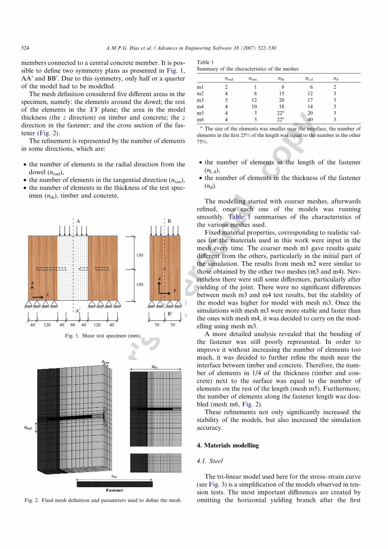
members connected to a central concrete member. It is pos-sible to define two symmetry plans as presented in Fig. 1,AA 0 and BB 0. Due to this symmetry, only half or a quarterof the model had to be modelled.

The mesh definition considered five different areas in thespecimen, namely: the elements around the dowel; the restof the elements in the XY plane; the area in the modelthickness (the z direction) on timber and concrete; the z

direction in the fastener; and the cross section of the fas-tener (Fig. 2).

The refinement is represented by the number of elementsin some directions, which are:

• the number of elements in the radial direction from thedowel (nrad),

• the number of elements in the tangential direction (ntan),• the number of elements in the thickness of the test spec-

imen (nth), timber and concrete,

• the number of elements in the length of the fastener(nl, d),

• the number of elements in the thickness of the fastener(nd).

The modelling started with coarser meshes, afterwardsrefined, once each one of the models was runningsmoothly. Table 1 summarises of the characteristics ofthe various meshes used.

Fixed material properties, corresponding to realistic val-ues for the materials used in this work were input in themesh every time. The coarser mesh m1 gave results quitedifferent from the others, particularly in the initial part ofthe simulation. The results from mesh m2 were similar tothose obtained by the other two meshes (m3 and m4). Nev-ertheless there were still some differences, particularly afteryielding of the joint. There were no significant differencesbetween mesh m3 and m4 test results, but the stability ofthe model was higher for model with mesh m3. Once thesimulations with mesh m3 were more stable and faster thanthe ones with mesh m4, it was decided to carry on the mod-elling using mesh m3.

A more detailed analysis revealed that the bending ofthe fastener was still poorly represented. In order toimprove it without increasing the number of elements toomuch, it was decided to further refine the mesh near theinterface between timber and concrete. Therefore, the num-ber of elements in 1/4 of the thickness (timber and con-crete) next to the surface was equal to the number ofelements on the rest of the length (mesh m5). Furthermore,the number of elements along the fastener length was dou-bled (mesh m6, Fig. 2).

These refinements not only significantly increased thestability of the models, but also increased the simulationaccuracy.

4. Materials modelling

4.1. Steel

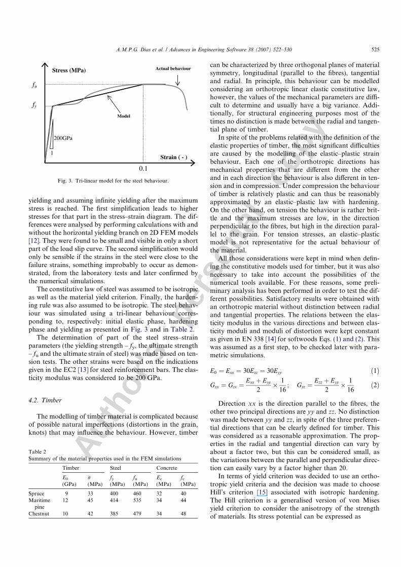
The tri-linear model used here for the stress–strain curve(see Fig. 3) is a simplification of the models observed in ten-sion tests. The most important differences are created byomitting the horizontal yielding branch after the first

A

A′

B

B′

40 120 40 60 40 120 40

150

150

70 70

x

z

x

y

Fig. 1. Shear test specimen (mm).

Fig. 2. Final mesh definition and parameters used to define the mesh.

Table 1Summary of the characteristics of the meshes

nrad ntan nth nl, d nd

m1 2 1 8 6 2m2 4 8 15 12 3m3 5 12 20 17 3m4 4 10 18 14 3m5 4 3 22a 20 3m6 4 3 22a 40 3

a The size of the elements was smaller near the interface, the number ofelements in the first 25% of the length was equal to the number in the other75%.

524 A.M.P.G. Dias et al. / Advances in Engineering Software 38 (2007) 522–530

Autho

r's

pers

onal

co

py

yielding and assuming infinite yielding after the maximumstress is reached. The first simplification leads to higherstresses for that part in the stress–strain diagram. The dif-ferences were analysed by performing calculations with andwithout the horizontal yielding branch on 2D FEM models[12]. They were found to be small and visible in only a shortpart of the load slip curve. The second simplification wouldonly be sensible if the strains in the steel were close to thefailure strains, something improbably to occur as demon-strated, from the laboratory tests and later confirmed bythe numerical simulations.

The constitutive law of steel was assumed to be isotropicas well as the material yield criterion. Finally, the harden-ing rule was also assumed to be isotropic. The steel behav-iour was simulated using a tri-linear behaviour corres-ponding to, respectively: initial elastic phase, hardeningphase and yielding as presented in Fig. 3 and in Table 2.

The determination of part of the steel stress–strainparameters (the yielding strength – fy, the ultimate strength– fu and the ultimate strain of steel) was made based on ten-sion tests. The other strains were based on the indicationsgiven in the EC2 [13] for steel reinforcement bars. The elas-ticity modulus was considered to be 200 GPa.

4.2. Timber

The modelling of timber material is complicated becauseof possible natural imperfections (distortions in the grain,knots) that may influence the behaviour. However, timber

can be characterized by three orthogonal planes of materialsymmetry, longitudinal (parallel to the fibres), tangentialand radial. In principle, this behaviour can be modelledconsidering an orthotropic linear elastic constitutive law,however, the values of the mechanical parameters are diffi-cult to determine and usually have a big variance. Addi-tionally, for structural engineering purposes most of thetimes no distinction is made between the radial and tangen-tial plane of timber.

In spite of the problems related with the definition of theelastic properties of timber, the most significant difficultiesare caused by the modelling of the elastic–plastic strainbehaviour. Each one of the orthotropic directions hasmechanical properties that are different from the otherand in each direction the behaviour is also different in ten-sion and in compression. Under compression the behaviourof timber is relatively plastic and can thus be reasonablyapproximated by an elastic–plastic law with hardening.On the other hand, on tension the behaviour is rather brit-tle and the maximum stresses are low, in the directionperpendicular to the fibres, but high in the direction paral-lel to the grain. For tension stresses, an elastic–plasticmodel is not representative for the actual behaviour ofthe material.

All those considerations were kept in mind when defin-ing the constitutive models used for timber, but it was alsonecessary to take into account the possibilities of thenumerical tools available. For these reasons, some preli-minary analysis has been performed in order to test the dif-ferent possibilities. Satisfactory results were obtained withan orthotropic material without distinction between radialand tangential properties. The relations between the elas-ticity modulus in the various directions and between elas-ticity moduli and moduli of distortion were kept constantas given in EN 338 [14] for softwoods Eqs. (1) and (2). Thiswas assumed as a first step, to be checked later with para-metric simulations.

E0 ¼ Exx ¼ 30Ezz ¼ 30Eyy ð1Þ

Gxy ¼ Gzx ¼Exx þ Eyy

2� 1

16; Gyz ¼

Ezz þ Eyy

2� 1

16ð2Þ

Direction xx is the direction parallel to the fibres, theother two principal directions are yy and zz. No distinctionwas made between yy and zz, in spite of the three preferen-tial directions that can be clearly defined for timber. Thiswas considered as a reasonable approximation. The prop-erties in the radial and tangential direction can vary byabout a factor two, but this can be considered small, asthe variations between the parallel and perpendicular direc-tion can easily vary by a factor higher than 20.

In terms of yield criterion was decided to use an ortho-tropic yield criteria and the decision was made to chooseHill’s criterion [15] associated with isotropic hardening.The Hill criterion is a generalised version of von Misesyield criterion to consider the anisotropy of the strengthof materials. Its stress potential can be expressed as

0.1

Strain ( - )

fu

fy

Stress (MPa) Actual behaviour

Model

1

200GPa

Fig. 3. Tri-linear model for the steel behaviour.

Table 2Summary of the material properties used in the FEM simulations

Timber Steel Concrete

E0

(GPa)�r(MPa)

fy

(MPa)fu

(MPa)Ec

(MPa)fc

(MPa)

Spruce 9 33 400 460 32 40Maritime

pine12 45 414 535 34 44

Chestnut 10 42 385 479 34 48

A.M.P.G. Dias et al. / Advances in Engineering Software 38 (2007) 522–530 525

Autho

r's

pers

onal

co

py

2�r2 ¼ ½a1ðry � rzÞ2 þ a2ðrz � rxÞ2 þ a3ðrx � ryÞ2

þ 3a4s2zx þ 3a5s

2yz þ 3a6s

2xy � ð3Þ

Considering the assumptions made above the parametersfrom Eq. (3) can be defined as

a1 ¼1

r90

�r

� �2þ 1

r90

�r

� �2� 1

r0

�r

� �2ð4Þ

a2 ¼1

r90

�r

� �2þ 1

r0

�r

� �2� 1

r90

�r

� �2ð5Þ

a3 ¼1

r0

�r

� �2þ 1

r90

�r

� �2� 1

r90

�r

� �2ð6Þ

a4 ¼2ffiffi3p

rv�r

� �2ð7Þ

a5 ¼2ffiffi3p

rv�r

� �2ð8Þ

a6 ¼2ffiffi3p

rv�r

� �2ð9Þ

where r0 is the yielding strength in the direction parallel tothe grain, r90 is the yielding strength in the direction per-pendicular to the grain, rv is the yield shear strength, �r isthe equivalent yielding strength for isotropic behaviour.The ratio between the yielding strengths and the equivalentyielding strength were defined according to:

r0

�r¼ 1;

r90

�r¼ 0:19;

ffiffiffi3p

rv

�r¼ 0:38 ð10Þ

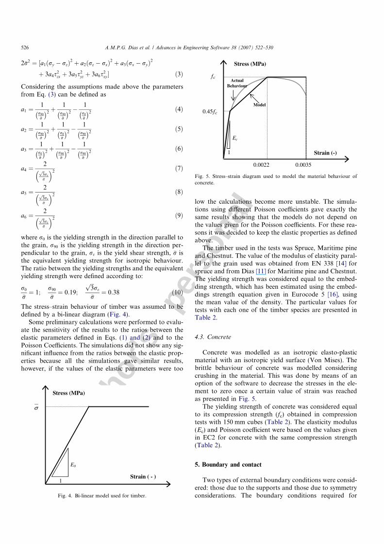
The stress–strain behaviour of timber was assumed to bedefined by a bi-linear diagram (Fig. 4).

Some preliminary calculations were performed to evalu-ate the sensitivity of the results to the ratios between theelastic parameters defined in Eqs. (1) and (2) and to thePoisson Coefficients. The simulations did not show any sig-nificant influence from the ratios between the elastic prop-erties because all the simulations gave similar results,however, if the values of the elastic parameters were too

low the calculations become more unstable. The simula-tions using different Poisson coefficients gave exactly thesame results showing that the models do not depend onthe values given for the Poisson coefficients. For these rea-sons it was decided to keep the elastic properties as definedabove.

The timber used in the tests was Spruce, Maritime pineand Chestnut. The value of the modulus of elasticity paral-lel to the grain used was obtained from EN 338 [14] forspruce and from Dias [11] for Maritime pine and Chestnut.The yielding strength was considered equal to the embed-ding strength, which has been estimated using the embed-dings strength equation given in Eurocode 5 [16], usingthe mean value of the density. The particular values fortests with each one of the timber species are presented inTable 2.

4.3. Concrete

Concrete was modelled as an isotropic elasto-plasticmaterial with an isotropic yield surface (Von Mises). Thebrittle behaviour of concrete was modelled consideringcrushing in the material. This was done by means of anoption of the software to decrease the stresses in the ele-ment to zero once a certain value of strain was reachedas presented in Fig. 5.

The yielding strength of concrete was considered equalto its compression strength (fc) obtained in compressiontests with 150 mm cubes (Table 2). The elasticity modulus(Ec) and Poisson coefficient were based on the values givenin EC2 for concrete with the same compression strength(Table 2).

5. Boundary and contact

Two types of external boundary conditions were consid-ered: those due to the supports and those due to symmetryconsiderations. The boundary conditions required for

Strain ( - )

σ

Stress (MPa)

E0

1

Fig. 4. Bi-linear model used for timber.

fc

0.45fc

Strain (-)

0.0035

Model

ActualBehaviour

0.0022

Ec

1

Stress (MPa)

Fig. 5. Stress–strain diagram used to model the material behaviour ofconcrete.

526 A.M.P.G. Dias et al. / Advances in Engineering Software 38 (2007) 522–530

Autho

r's

pers

onal

co

py

symmetry reasons were different for symmetry plane AA 0

and for symmetry plane BB 0 (Fig. 1). In principle, the com-patibility of displacements in the symmetry plane AA 0

require zero translation in z direction and zero rotationin x and y directions. However, as the elements used donot have rotation degrees of freedom, only the translationhad to be restrained. In the symmetry plane BB 0 the sameconsiderations would force the translation in y directionand the rotation in x and z directions to be zero. Once moredue to the degrees of freedom of element used, only thetranslation was restrained.

In the model, the supports were simulated consideringprescribed values of zero displacements for the three trans-lations in all the nodes that correspond to support areas inthe shear tests (the nodes in the timber elements base).Using this approach, a rigid connection was assumedbetween the specimen and the supports and at the sametime no horizontal displacement was allowed in the bottomof the timber blocks.

The loads were introduced by increasing controlled dis-placements applied on all the nodes in the top of the con-crete element, as done in the laboratory tests. The step ofload increase was defined in order to obtain a well definedload slip curve. For that reason the steps in the first part ofthe loading (up to 4 mm), were smaller than that after thispoint when the load slip behaviour is more linear.

5.1. Contact

The interaction between the different members wasalways modelled with deformable contact elements. Con-tact could occur between: the timber and concrete in theinterface, the fastener and the concrete around the fasteneron the concrete side and finally the fastener and the timberaround the fastener on the timber side. According to thenumerical procedure used, contact can occur between anycontact body of timber against any contact body of steeland the other way around, the same occurs with timber–concrete and concrete–steel contact.

The contact was simulated using the direct constrainsmethod. In this method, when a node of a body contactsanother body, a multipoint constrain is imposed. This con-strain allows the node to slide on the contacted segment,forcing it to be on that segment. During the iteration pro-cedure, a node is allowed to slide from one segment toanother, changing the nodes that were previously associ-ated with the constrain condition. The changing of thenodes takes place when the node passes the end of the seg-ment by a distance higher than the contact tolerance.

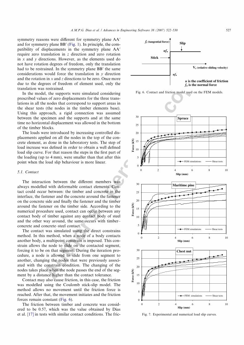
Contact may also cause friction, in this case, the frictionwas modelled using the Coulomb stick-slip model. Themethod allows no movement until the friction force isreached. After that, the movement initiates and the frictionforces remain constant (Fig. 6).

The friction between timber and concrete was consid-ered to be 0.57, which was the value obtained by Diaset al. [17] in tests with similar contact conditions. The fric-

Stick

Slip

Vr (relative sliding velocity)

ufn

u is the coefficient of frictionfn is the normal force

ft (tangential force)

ufn

Fig. 6. Contact and friction model used on the FEM models.

Spruce

0

5

10

15

20

25

30

Slip (mm)

For

ce (

kN)

FEM simulations Shear tests

Maritime pine

0

5

10

15

20

25

30

For

ce (

kN)

FEM simulations Shear tests

Chest nut

0

5

10

15

20

25

30

0 10Slip (mm)

Slip (mm)

For

ce (

kN)

FEM simulations Shear tests

2 4 6 8

0 102 4 6 8

0 102 4 6 8

Fig. 7. Experimental and numerical load slip curves.

A.M.P.G. Dias et al. / Advances in Engineering Software 38 (2007) 522–530 527

Autho

r's

pers

onal

co

py

tion between timber and steel was 0.50 [7]. During the sheartests no movement was observed between concrete andsteel, in order to simulate that behaviour, a value of 0.9was given to the friction coefficient between concrete andsteel.

6. Results from the numerical simulations

The model developed showed a good stability up to aslip value of 10 mm. For higher deformations the simula-tions became unstable. Therefore, the results presentedare for slip values lower than 10 mm. Fig. 7 presents theload slip curves obtained in the tests [10,11] as well as theload slip curve obtained in the numerical simulations.

The global shape of the load slip curve obtained in thetests is reasonably simulated by the FEM models (Fig. 7).The numerical prediction, however, over-estimates thejoint stiffness and strength. The overestimation in the load(or underestimation in the deformations) is almost con-stant from the initiation of yielding in the joint up to theend of the simulation. This indicates that the higher ulti-mate load carrying capacity is probably a consequencefrom an initial overestimation.

It is difficult to identify exactly all the causes of these dif-ferences. Part of them, however, are probably related withthe model used to simulate the timber behaviour. The bi-linear model of timber assumes linear elastic behaviourup to yielding but the elastic stiffness is usually determinedfor loads lower than 40% of the ultimate load carryingcapacity. On the other hand the actual material behaviour

of timber is non-linear particularly after 40% of the loadcarrying capacity is reached. Therefore, the loads can beoverestimated and the displacements underestimated.Besides, the assumption of a yielding strength equal tothe embedding strength of timber may be unrealistic lead-ing to high values of the strength in the simulations.

From the three timber species tested, it is clear that theinitial deformation is better predicted for the simulationswith harder woods: Maritime pine and Chestnut. On thatsituation the pre-drilled holes are more precise resultingin lower initial deformations, therefore the higher differ-ences obtained for the test specimens with Spruce are alsorelated with the hole clearance.

Another important result obtained from the simulationsis the pattern of stress distribution inside the test speci-mens. This information is difficult to compare with the phe-nomena observed in the tests, but it can somehow berelated to the deformations observed in the tests. It is pos-sible to evaluate the embedment length in the shear teststhrough the embedment deformation. In addition, thesplitting under the fastener can be compared with the ten-sion stresses perpendicular to the grain under the fasteneron the timber surface.

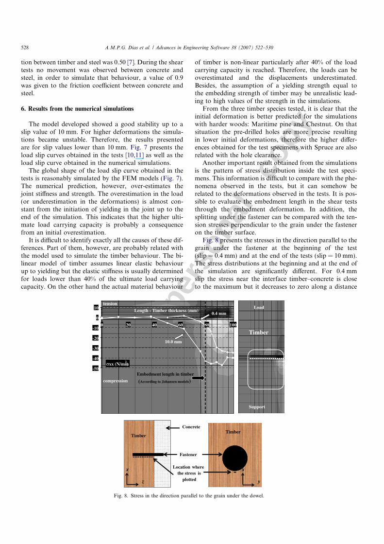
Fig. 8 presents the stresses in the direction parallel to thegrain under the fastener at the beginning of the test(slip = 0.4 mm) and at the end of the tests (slip = 10 mm).The stress distributions at the beginning and at the end ofthe simulation are significantly different. For 0.4 mmslip the stress near the interface timber–concrete is closeto the maximum but it decreases to zero along a distance

Support

Timber

Load

-50

-40

-30

-20

-10

0

10

0 20 40 60 80 100

Length - Timber thickness (mm)

σxx (N/mm2)

Embedment length in timber

(According to Johansen models)

10.0 mm

0.4 mm

compression

tension

Fastener

Concrete

Location where the stress is

plotted

x

z

Timber

x

y

Timber

Fig. 8. Stress in the direction parallel to the grain under the dowel.

528 A.M.P.G. Dias et al. / Advances in Engineering Software 38 (2007) 522–530

Autho

r's

pers

onal

co

py

of approximately 25 mm. It decreases slowly in the firsthalf of that length, but fast in the second half. The stressdistribution in the last iteration (10 mm) shows values closeto the maximum stress in the first 20 mm (next to the inter-face timber–concrete) followed by a significant decrease. Inthe last 2/5 of the fastener length the stresses are stable andalmost zero. The embedment length obtained from a plas-tic limit calculation considering timber–concrete models(both with elastic perfect plastic behaviour, according toJohansen theory [18]) is also drawn, and is well in line withthe length where the maximum stresses are obtained for10 mm slip.

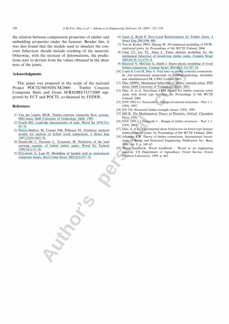
In order to evaluate the stresses perpendicular to thegrain (ryy) that take place under the dowel, they were plot-ted along the timber height, from the fastener up to thesupports of the test specimen (Fig. 9). These stresses arepresented in the iteration where the maximum tensionstress were obtained, corresponding to a slip of 4 mm.

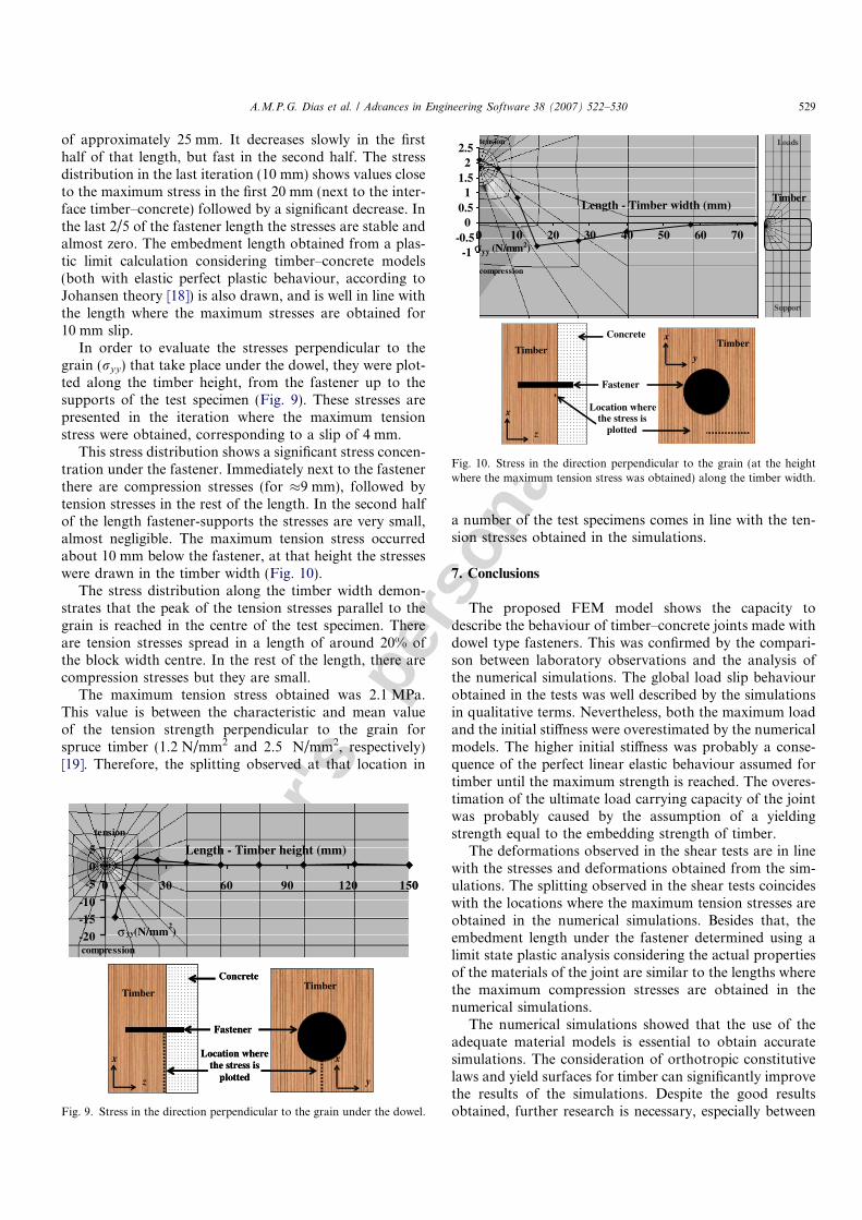
This stress distribution shows a significant stress concen-tration under the fastener. Immediately next to the fastenerthere are compression stresses (for �9 mm), followed bytension stresses in the rest of the length. In the second halfof the length fastener-supports the stresses are very small,almost negligible. The maximum tension stress occurredabout 10 mm below the fastener, at that height the stresseswere drawn in the timber width (Fig. 10).

The stress distribution along the timber width demon-strates that the peak of the tension stresses parallel to thegrain is reached in the centre of the test specimen. Thereare tension stresses spread in a length of around 20% ofthe block width centre. In the rest of the length, there arecompression stresses but they are small.

The maximum tension stress obtained was 2.1 MPa.This value is between the characteristic and mean valueof the tension strength perpendicular to the grain forspruce timber (1.2 N/mm2 and 2.5 N/mm2, respectively)[19]. Therefore, the splitting observed at that location in

a number of the test specimens comes in line with the ten-sion stresses obtained in the simulations.

7. Conclusions

The proposed FEM model shows the capacity todescribe the behaviour of timber–concrete joints made withdowel type fasteners. This was confirmed by the compari-son between laboratory observations and the analysis ofthe numerical simulations. The global load slip behaviourobtained in the tests was well described by the simulationsin qualitative terms. Nevertheless, both the maximum loadand the initial stiffness were overestimated by the numericalmodels. The higher initial stiffness was probably a conse-quence of the perfect linear elastic behaviour assumed fortimber until the maximum strength is reached. The overes-timation of the ultimate load carrying capacity of the jointwas probably caused by the assumption of a yieldingstrength equal to the embedding strength of timber.

The deformations observed in the shear tests are in linewith the stresses and deformations obtained from the sim-ulations. The splitting observed in the shear tests coincideswith the locations where the maximum tension stresses areobtained in the numerical simulations. Besides that, theembedment length under the fastener determined using alimit state plastic analysis considering the actual propertiesof the materials of the joint are similar to the lengths wherethe maximum compression stresses are obtained in thenumerical simulations.

The numerical simulations showed that the use of theadequate material models is essential to obtain accuratesimulations. The consideration of orthotropic constitutivelaws and yield surfaces for timber can significantly improvethe results of the simulations. Despite the good resultsobtained, further research is necessary, especially between

-20-15-10

-505

0 30 60 90 120 150

Length - Timber height (mm)

yy(N/mm2)

tension

compression

x

z

x

y

TimberTimber

Fastener

Concrete

Location where the stress is

plotted

-20 σ-15-10

-505

0 30 60 90 120 150

Length - Timber height (mm)

yy(N/mm2)

tension

compression

x

z

x

y

TimberTimber

Fastener

Concrete

Location where the stress is

plotted

Fig. 9. Stress in the direction perpendicular to the grain under the dowel.

Loads

Timber

Support

-1-0.5

00.5

11.5

22.5

0σ

10 20 30 40 50 60 70

Length - Timber width (mm)

yy (N/mm2)

compression

tension

Fastener

Concrete

Location where the stress is

plotted

x

z

Timberx

y

Timber

Fig. 10. Stress in the direction perpendicular to the grain (at the heightwhere the maximum tension stress was obtained) along the timber width.

A.M.P.G. Dias et al. / Advances in Engineering Software 38 (2007) 522–530 529

Autho

r's

pers

onal

co

py

the relation between compression properties of timber andembedding properties under the fastener. Besides this, itwas also found that the models used to simulate the con-crete behaviour should include crushing of the material.Otherwise, with the increase of deformations, the predic-tions start to deviate from the values obtained in the sheartests of the joints.

Acknowledgments

This paper was prepared in the scope of the nationalProject POCTI/36039/ECM/2000 – Timber ConcreteComposite Slabs and Grant SFRH/BD/3327/2000 sup-ported by FCT and POCTI, co-financed by FEDER.

References

[1] Van der Linden MLR. Timber–concrete composite floor systems.PhD thesis, Delft University of Technology, Delft, 1999.

[2] Foschi RO. Load-slip characteristics of nails. Wood Sci 1974;7(1):69–76.

[3] Patton-Mallory M, Cramer SM, Pellicane PJ. Nonlinear materialmodels for analysis of bolted wood connections. J Struct Eng1997;123(8):1063–70.

[4] Daudeville L, Davenne L, Yasumura M. Prediction of the loadcarrying capacity of bolted timber joints. Wood Sci Technol1999;33(1):15–29.

[5] El-Lobody E, Lam D. Modelling of headed stud in steel-precastcomposite beams. Steel Comp Struct 2002;2(5):355–78.

[6] Guan Z, Rodd P. Dvw-Local Reinforcement for Timber Joints. JStruct Eng 2001:894–900.

[7] Van de Kuilen JWG, Dejong M. 3D-numerical modelling of DVW-reinforced joints. In: Proceedings of 8th WCTE Finland; 2004.

[8] Chen CJ, Lee TL, Jiang L. Finite element modelling for themechanical behaviour of dowel-type timber joints. Comput Struct2003;81(30–31):2731–8.

[9] Kharouf N, McClure G, Smith I. Elasto-plastic modelling of woodbolted connections. Comput Struct 2003;81(8–11):747–54.

[10] Lopes S, Cruz H, Dias A. Trial tests on timber–concrete connections.In: 2nd international symposium on building pathology, durabilityand rehabilitation-CIB, LNEC-Lisbon; 2003.

[11] Dias AMPG. Mechanical behaviour of timber–concrete joints. PhDthesis, Delft University of Technology, Delft; 2005.

[12] Dias, A. et al. Non-linear FEM models for timber–concrete jointsmade with dowel type fasteners. In: Proceedings of 8th WCTEFinland; 2004.

[13] ENV 1992-1-1. Eurocode 2 – Design of concrete structures – Part 1–1.CEN, 1997.

[14] EN 338, Structural timber-strength classes. CEN, 1995.[15] Hill R. The Mathematical Theory of Plasticity. Oxford: Clarendon

Press; 1950.[16] ENV 1995-1-1 Eurocode 5 – Design of timber structures – Part 1–1.

CEN, 2003.[17] Dias, A. et al., Experimental shear-friction test on dowel type fastener

timber–concrete joints. In: Proceedings of 8th WCTE Finland, 2004.[18] Johansen KW. Theory of timber connections. International Associ-

ation of Bridge and Structural Engineering. Publication No.; Bern;1949, vol. 9. p. 249–62.

[19] Wood handbook, Wood handbook – Wood as an engineeringmaterial. US Department of Agriculture, Forest Service, ForestProducts Laboratory; 1999. p. 463.

530 A.M.P.G. Dias et al. / Advances in Engineering Software 38 (2007) 522–530