ITB J. ICT, Vol. 6, No. 2, 2012, 131-150 131 Received November 14 th , 2011, Revised February 26 th , 2012, Accepted for publication September 22 nd , 2012. Copyright © 2012 Published by LPPM ITB,ISSN: 1978-3086, DOI: 10.5614/itbj.ict.2012.6.2.3 A New RTL Design Approach for a DCT/IDCT-Based Image Compression Architecture Using the mCBE Algorithm Rachmad Vidya Wicaksana Putra, Rella Mareta, Nurfitri Anbarsanti & Trio Adiono IC Design Laboratory, Electrical Engineering, School of Electrical Engineering and Informatics, Institut Teknologi Bandung, Jalan Ganesha 10, Bandung 40132, Indonesia Email: [email protected], [email protected] Abstract. In the literature, several approaches of designing a DCT/IDCT-based image compression system have been proposed. In this paper, we present a new RTL design approach with as main focus developing a DCT/IDCT-based image compression architecture using a self-created algorithm. This algorithm can efficiently minimize the amount of shifter-adders to substitute multipliers. We call this new algorithm the multiplication from Common Binary Expression (mCBE) Algorithm. Besides this algorithm, we propose alternative quantization numbers, which can be implemented simply as shifters in digital hardware. Mostly, these numbers can retain a good compressed-image quality compared to JPEG recommendations. These ideas lead to our design being small in circuit area, multiplierless, and low in complexity. The proposed 8-point 1D-DCT design has only six stages, while the 8-point 1D-IDCT design has only seven stages (one stage being defined as equal to the delay of one shifter or 2-input adder). By using the pipelining method, we can achieve a high-speed architecture with latency as a trade-off consideration. The design has been synthesized and can reach a speed of up to 1.41ns critical path delay (709.22MHz). Keywords: DCT/IDCT architecture; low complexity; mCBE Algorithm; multiplierless; new RTL design approach. 1 Introduction Many kinds of digital image and video processing techniques have been proposed in the literature. Most of them, require discrete cosine transform (DCT). In this paper, we will discuss DCT-based image compression, one of the most interesting topics in image processing. Actually, DCT is not an algorithm specifically developed for image compression. But, we can take advantage of DCT theory to support well-performing image compression [1]. In the past years, many DCT-based researches have been conducted. Loeffler, C., et al. [2] proposed a low complexity DCT using the Flow-Graph Algorithm. This design requires 11 multiplications and 29 additions. Jeong, et al. [3]

Welcome message from author
This document is posted to help you gain knowledge. Please leave a comment to let me know what you think about it! Share it to your friends and learn new things together.
Transcript
ITB J. ICT, Vol. 6, No. 2, 2012, 131-150 131
Received November 14th, 2011, Revised February 26th, 2012, Accepted for publication September 22nd, 2012. Copyright © 2012 Published by LPPM ITB,ISSN: 1978-3086, DOI: 10.5614/itbj.ict.2012.6.2.3
A New RTL Design Approach for a DCT/IDCT-Based
Image Compression Architecture Using the mCBE
Algorithm
Rachmad Vidya Wicaksana Putra, Rella Mareta, Nurfitri Anbarsanti
& Trio Adiono
IC Design Laboratory, Electrical Engineering, School of Electrical Engineering and
Informatics, Institut Teknologi Bandung, Jalan Ganesha 10, Bandung 40132, Indonesia
Email: [email protected], [email protected]
Abstract. In the literature, several approaches of designing a DCT/IDCT-based
image compression system have been proposed. In this paper, we present a new
RTL design approach with as main focus developing a DCT/IDCT-based image
compression architecture using a self-created algorithm. This algorithm can
efficiently minimize the amount of shifter-adders to substitute multipliers. We
call this new algorithm the multiplication from Common Binary Expression
(mCBE) Algorithm. Besides this algorithm, we propose alternative quantization
numbers, which can be implemented simply as shifters in digital hardware.
Mostly, these numbers can retain a good compressed-image quality compared to
JPEG recommendations. These ideas lead to our design being small in circuit
area, multiplierless, and low in complexity. The proposed 8-point 1D-DCT
design has only six stages, while the 8-point 1D-IDCT design has only seven
stages (one stage being defined as equal to the delay of one shifter or 2-input
adder). By using the pipelining method, we can achieve a high-speed architecture
with latency as a trade-off consideration. The design has been synthesized and
can reach a speed of up to 1.41ns critical path delay (709.22MHz).
Keywords: DCT/IDCT architecture; low complexity; mCBE Algorithm; multiplierless;
new RTL design approach.
1 Introduction
Many kinds of digital image and video processing techniques have been
proposed in the literature. Most of them, require discrete cosine transform
(DCT). In this paper, we will discuss DCT-based image compression, one of the
most interesting topics in image processing. Actually, DCT is not an algorithm
specifically developed for image compression. But, we can take advantage of
DCT theory to support well-performing image compression [1].
In the past years, many DCT-based researches have been conducted. Loeffler,
C., et al. [2] proposed a low complexity DCT using the Flow-Graph Algorithm.
This design requires 11 multiplications and 29 additions. Jeong, et al. [3]
132 Rachmad Vidya Wicaksana Putra, et. al.
proposed a low-power multiplierless DCT architecture using image data
correlation (cordic). Ruiz, et al. [4] proposed a high-throughput parallel-pipeline
2D-DCT/IDCT processor. Heyne, et al. [5] proposed a combination of the
Loeffler DCT and cordic method, which requires 38 adders and 16 shifters for
8-point 1D-DCT and consists of 3 cordic blocks with several adders. Each block
consists of an iterative shift-add operation and the longest path takes three
iterations. Therefore, its longest path has an 8-stage delay (we define one stage
as the delay of one shifter or 2-input adder). Byoung-Il Kim, et al. [6] have
proposed a low-power multiplierless DCT for image/video coders.
Subramanian, et al. [7] have proposed a VLSI implementation of a fully
pipelined multiplierless 2D-DCT/IDCT architecture for JPEGs.
In this paper, we propose a new approach of designing a DCT/IDCT-based
image compression architecture. The main focus of our research was to develop
the architecture by using a self-created algorithm that can efficiently minimize
the amount of shifter-adders to substitute constant multipliers. We named it:
multiplication from Common Binary Expression (mCBE) Algorithm. We also
propose alternative quantization numbers, which can be implemented simply as
shifters. Mostly, these numbers can retain a good compressed image quality
compared to JPEG recommendations. We had three objectives. Firstly, the
design had to be able to operate well, producing a good compressed image
quality represented by Peak-to-peak Signal to Noise Ratio (PSNR) and Mean
Square Error (MSE) values. Secondly, the design had to have less than 8-stage
delay of flow-graph architecture without iterations for 8-point 1D-DCT/IDCT.
Thirdly, the design had to have a small circuit area, be multiplierless, and have
low complexity, so that it can be implemented easily in digital hardware.
This paper is organized in a number of sections. First, the introduction section
briefly introduces: (1) the importance of DCT theory in image compression
systems, (2) several past researches about DCT-based image compression
systems, and (3) the main points of the proposed design. This section is
followed by a brief explanation of DCT/IDCT theory and its usage in image
compression systems. The next section is about the proposed design. Here, we
explain our design approach and its implementation in detail. This section is
followed by the synthesis and analysis regarding our proposal. We also compare
the proposed design with other design methods. In the following section, we
explain the simulation and FPGA implementation. Finally, this section is
followed by conclusion and references, respectively.
2 Fundamental Theory
In designing a DCT/IDCT-based image compression system, we need to use
DCT/IDCT formulations and quantification-dequantification processing [8].
DCT/IDCT-Based Img. Comp. Arch. Using mCBE Algorithm 133
2.1 Discrete Cosine Transform Formulation
The equation of 1-Dimension N-points DCT is formulated as:
1
0
)(2
)12(cos)()(
N
x
xN
uxfuuZ
,
0 2
0 1
uforN
uforNu (1)
2.2 Inverse Discrete Cosine Transform Formulation
The equation of 1-Dimension N-points Inverse DCT is formulated as:
1
0
)(2
)12(cos)()(
N
x
uN
uxZuxf
,
0 2
0 1
uforN
uforNu (2)
2.3 Basic DCT/IDCT-Based Image Compression System
The main idea behind this image compression system is to reduce the image
data size without significantly reducing image quality to the human eye. This
technique will remove the least significant (high-frequency) information data
from the image. The most significant information data usually have a low
frequency. For the human eye it is more difficult to see differences in high
frequencies than in low frequencies. Therefore, by eliminating the higher
frequencies we can significantly reduce the image size without abandoning
image quality.
The input and output data of the DCT/IDCT-based compression system can be
provided by using the YCbCr format. Input image data in JPEG format are
converted to YCbCr format, which has three macroblock components: Y
(luminance), Cb (chrominance blue), and Cr (chrominance red). Each
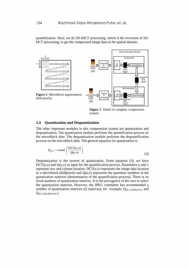
component is computed based on microblock segmentation (8x8pixels), as
shown in Figure 1. The inverse process is applied to the output data of the
system in order to get the actual image (JPEG format).Therefore, by combining
Eqs. (1) and (2) with microblock characters, we can compute 64-point data in a
2D-DCT/IDCT process from an 8-point input 1D-DCT only.
Figure 2 shows the details of the process of the complete compression system.
In the complete compression system, first the image data will be represented as
spatial domain data. These data will be transformed to frequency domain data
using 2D-DCT processing. Then, we organize the frequency domain data in
term of importance. Thus, we can eliminate the high-frequency data using
134 Rachmad Vidya Wicaksana Putra, et. al.
quantification. Next, we do 2D-IDCT processing, which is the inversion of 2D-
DCT processing, to get the compressed image data in the spatial domain.
Figure 1 Microblock segmentation
(8x8-pixels).
Figure 2 Detail of complete compression
system.
2.4 Quantization and Dequantization
The other important modules in this compression system are quantization and
dequantization. The quantization module performs the quantification process on
the microblock data. The dequantization module performs the dequantification
process on the microblock data. The general equation for quantization is:
),(
),(
vuQ
vuDCTroundQDCT
(3)
Dequantization is the inverse of quantization. From equation (3), we have
DCT(u,v) and Q(u,v) as input for the quantification process. Parameters u and v
represent row and column location. DCT(u,v) represents the image data location
in a microblock (8x8pixels) and Q(u,v) represents the quantizer numbers in the
quantization matrices (denominators of the quantification process). There is no
fixed numbers of quantization matrices. It is the prerogative of the user to select
the quantization matrices. However, the JPEG committee has recommended a
number of quantization matrices (Q matrices), for example, Q50_LUMINANCE and
Q50_CHROMINANCE:
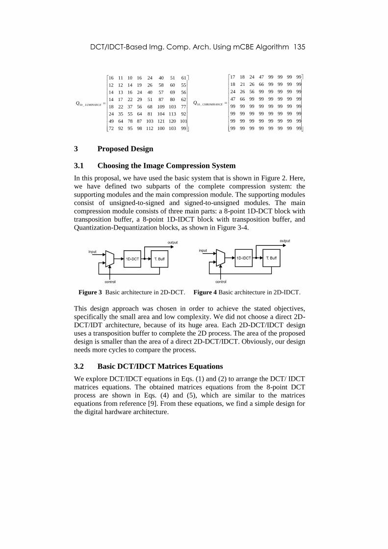
DCT/IDCT-Based Img. Comp. Arch. Using mCBE Algorithm 135
9910310011298959272
10112012110387786449
921131048164553524
771031096856372218
6280875129221714
5669574024161314
5560582619141212
6151402416101116
_50 LUMINANCEQ
9999999999999999
9999999999999999
9999999999999999
9999999999999999
9999999999996647
9999999999562624
9999999966262118
9999999947241817
_50 ECHROMINANCQ
3 Proposed Design
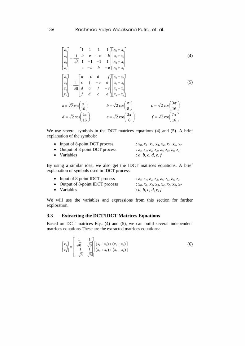
3.1 Choosing the Image Compression System
In this proposal, we have used the basic system that is shown in Figure 2. Here,
we have defined two subparts of the complete compression system: the
supporting modules and the main compression module. The supporting modules
consist of unsigned-to-signed and signed-to-unsigned modules. The main
compression module consists of three main parts: a 8-point 1D-DCT block with
transposition buffer, a 8-point 1D-IDCT block with transposition buffer, and
Quantization-Dequantization blocks, as shown in Figure 3-4.
Figure 3 Basic architecture in 2D-DCT. Figure 4 Basic architecture in 2D-IDCT.
This design approach was chosen in order to achieve the stated objectives,
specifically the small area and low complexity. We did not choose a direct 2D-
DCT/IDT architecture, because of its huge area. Each 2D-DCT/IDCT design
uses a transposition buffer to complete the 2D process. The area of the proposed
design is smaller than the area of a direct 2D-DCT/IDCT. Obviously, our design
needs more cycles to compare the process.
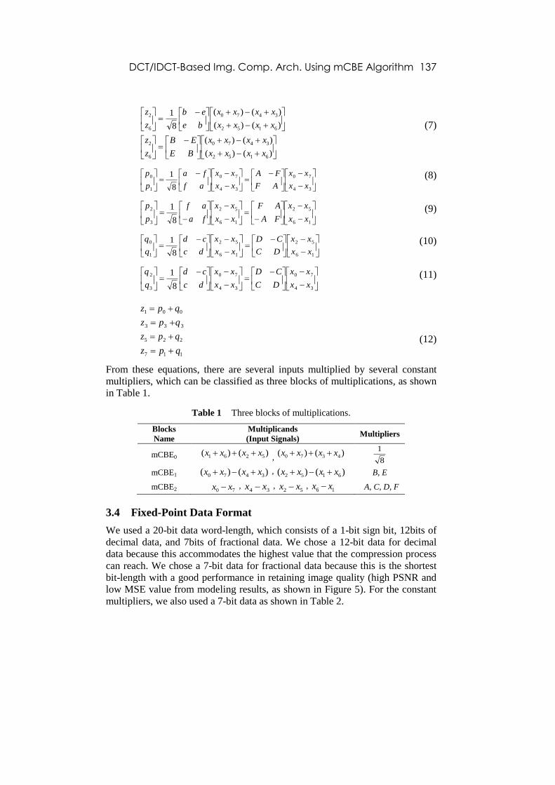
3.2 Basic DCT/IDCT Matrices Equations
We explore DCT/IDCT equations in Eqs. (1) and (2) to arrange the DCT/ IDCT
matrices equations. The obtained matrices equations from the 8-point DCT
process are shown in Eqs. (4) and (5), which are similar to the matrices
equations from reference [9]. From these equations, we find a simple design for
the digital hardware architecture.
136 Rachmad Vidya Wicaksana Putra, et. al.
43
52
61
70
6
4
2
0
1111
1111
8
1
xx
xx
xx
xx
ebbe
beeb
z
z
z
z
(4)
34
52
16
70
7
5
3
1
8
1
xx
xx
xx
xx
acdf
cfad
dafc
fdca
z
z
z
z
(5)
16cos2
a
8cos2
b
16
3cos2
c
16
5cos2
d
8
3cos2
e
16
7cos2
f
We use several symbols in the DCT matrices equations (4) and (5). A brief
explanation of the symbols:
Input of 8-point DCT process : x0, x1, x2, x3, x4, x5, x6, x7
Output of 8-point DCT process : z0, z1, z2, z3, z4, z5, z6, z7
Variables : a, b, c, d, e, f
By using a similar idea, we also get the IDCT matrices equations. A brief
explanation of symbols used in IDCT process:
Input of 8-point IDCT process : z0, z1, z2, z3, z4, z5, z6, z7
Output of 8-point IDCT process : x0, x1, x2, x3, x4, x5, x6, x7
Variables : a, b, c, d, e, f
We will use the variables and expressions from this section for further
exploration.
3.3 Extracting the DCT/IDCT Matrices Equations
Based on DCT matrices Eqs. (4) and (5), we can build several independent
matrices equations.These are the extracted matrices equations:
)()(
)()(
8
1
8
18
1
8
1
4370
5261
4
0
xxxx
xxxx
z
z (6)
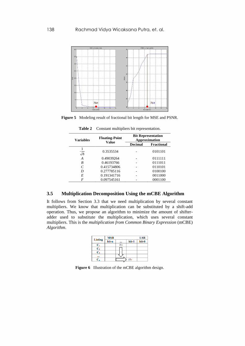
DCT/IDCT-Based Img. Comp. Arch. Using mCBE Algorithm 137
)()(
)()(
)()(
)()(
8
1
6152
3470
6
2
6152
3470
6
2
xxxx
xxxx
BE
EB
z
z
xxxx
xxxx
be
eb
z
z
(7)
34
70
34
70
1
0
8
1
xx
xx
AF
FA
xx
xx
af
fa
p
p (8)
16
52
16
52
3
2
8
1
xx
xx
FA
AF
xx
xx
fa
af
p
p (9)
16
52
16
52
1
0
8
1
xx
xx
DC
CD
xx
xx
dc
cd
q
q (10)
34
70
34
70
3
2
8
1
xx
xx
DC
CD
xx
xx
dc
cd
q
q (11)
(12)
From these equations, there are several inputs multiplied by several constant
multipliers, which can be classified as three blocks of multiplications, as shown
in Table 1.
Table 1 Three blocks of multiplications.
Blocks
Name
Multiplicands
(Input Signals) Multipliers
mCBE0 )()( 5261 xxxx ,
)()( 4370 xxxx 8
1
mCBE1 )()( 3470 xxxx , )()( 6152 xxxx B, E
mCBE2 70 xx ,
34 xx ,
52 xx ,
16 xx A, C, D, F
3.4 Fixed-Point Data Format
We used a 20-bit data word-length, which consists of a 1-bit sign bit, 12bits of
decimal data, and 7bits of fractional data. We chose a 12-bit data for decimal
data because this accommodates the highest value that the compression process
can reach. We chose a 7-bit data for fractional data because this is the shortest
bit-length with a good performance in retaining image quality (high PSNR and
low MSE value from modeling results, as shown in Figure 5). For the constant
multipliers, we also used a 7-bit data as shown in Table 2.
001 qpz 333 qpz 225 qpz
117 qpz
138 Rachmad Vidya Wicaksana Putra, et. al.
Figure 5 Modeling result of fractional bit length for MSE and PSNR.
Table 2 Constant multipliers bit representation.
Variables Floating-Point
Value
Bit Representation
Approximation
Decimal Fractional
8
1 0.3535534 - 0101101
A 0.49039264 - 0111111
B 0.46193766 - 0111011
C 0.415734806 - 0110101
D 0.277785116 - 0100100
E 0.191341716 - 0011000
F 0.097545161 - 0001100
3.5 Multiplication Decomposition Using the mCBE Algorithm
It follows from Section 3.3 that we need multiplication by several constant
multipliers. We know that multiplication can be substituted by a shift-add
operation. Thus, we propose an algorithm to minimize the amount of shifter-
adder used to substitute the multiplication, which uses several constant
multipliers. This is the multiplication from Common Binary Expression (mCBE)
Algorithm.
Figure 6 Illustration of the mCBE algorithm design.

DCT/IDCT-Based Img. Comp. Arch. Using mCBE Algorithm 139
Here, we present the mCBE Algorithm:
i. Listing of all constants (C1-n) which are used to multiply the same input,
then produce a table as shown in Figure 6.
ii. Choose and classify every constant which has bit value 1, more or equal to
70% from its bit’s amount. There will be two groups:
a. Group of [≥70%].
b. Group of [<70%].
iii. Suppose there are 2 groups.
a. Group of [≥70%] : Group A.
a.1 If only one constant fits in Group A, then:
Find out the most significant bit that contains the value of 1.
If the position is bit-m, choose bit-(m+1) as MostShiftBit.
Then, determine the SubShiftBit to complete the substraction
operation in order to get the desired result.
a.2 If there are several constants that fit in Group A, then:
For every constant, find out the most significant bit that
contains the value of 1.
If the position is bit-m, choose bit-(m+1) as MostShiftBit.
Then, determine the SubShiftBit to complete the substraction
operation in order to get the desired result.
If it is possible to use the same MostShiftBit or SubShiftBit, then
use them together to fit other constants.
b. Group of [<70%] : Group B.
b.1 Find out the most appeared value of 1 for Vv (vertical view), and
call it VvShiftBit. If there are several bits that fit, choose one.
b.2 From the chosen VvShiftBit point, find the most appeared bit value
of 1 for the corresponding Hv (horizontal view). We call this bit
HvShiftBit. There are three possible conditions: single HvShiftBit
found, several HvShiftBits found, or no HvShiftBit found.
b.2.1 If there is a single HvShiftBit, then:
Choose this bit as AddShiftBit to the chosen VvShiftBit.
Then, still with the same VvShiftBit, check again from
step (b.2) for unselected bits.
b.2.2 If there are several HvShiftBits, then:
Check whether between those HvShiftBits (Two or more
HvShiftBits are grouped as HvShiftBitsG) there is a mutual
inter-Hv relation (in the same constant).
If yes, then:
Choose the bit which has the least inter-Hv relation in
HvShiftBitsG as AddShiftBit to the chosen VvShiftBit.
If no, then:
Choose one as AddShiftBit to the chosen VvShiftBit.

140 Rachmad Vidya Wicaksana Putra, et. al.
b.2.3 If there is no HvShiftBit, then:
Continue to step (iv).
iv. Loop from step (iii) until all values 1 are represented as MostShiftBit,
VvShiftBit, SubShiftBit, or AddShifBit.
v. Design a butterfly-like flow-graph using chosen MostShiftBit, VvShiftBit,
SubShiftBit, or AddShifBit.
Notes:
Ci : Constant multiplier number i. Vv : Vertical view relation. Hv : Horizontal view relation. MostShiftBit : Biggest shifting bit value: its shifting result will be
substracted from another signal (usually SubShiftBit). VvShiftBit : Most appeared bit value 1 in vertical bit order, which is
used as shifting bit. HvShiftBit : Most appeared bit value 1 in inter-Hv relation to
VvShiftBit. HvShiftBitsG : Group of several HvShiftBits. AddShiftBit : The bit which is chosen as shifter bit and its shifting
output will be added to the result of VvShiftBit or another
AddShiftBit output. SubShiftBit : The bit which can be partner of MostShiftBit to complete
the substraction operation.
3.6 Implementation of the mCBE Algorithm
3.6.1 Basic mCBE Building Blocks
Implementation of the mCBE Algorithm occurs inside the multiplication block.
From Table 1, we get three blocks (mCBE0, mCBE1, and mCBE2).
a. The mCBE0 Block
Table 3 shows an illustration of the mCBE0 block design.
Table 3 Constant bit representation.
Variables Bit Representation
6 5 4 3 2 1 0
8
1 0 1 0 1 1 0 1
VvShiftBit0-1 AddShiftBit0-1
Then, we get the following architecture (Figure 7):
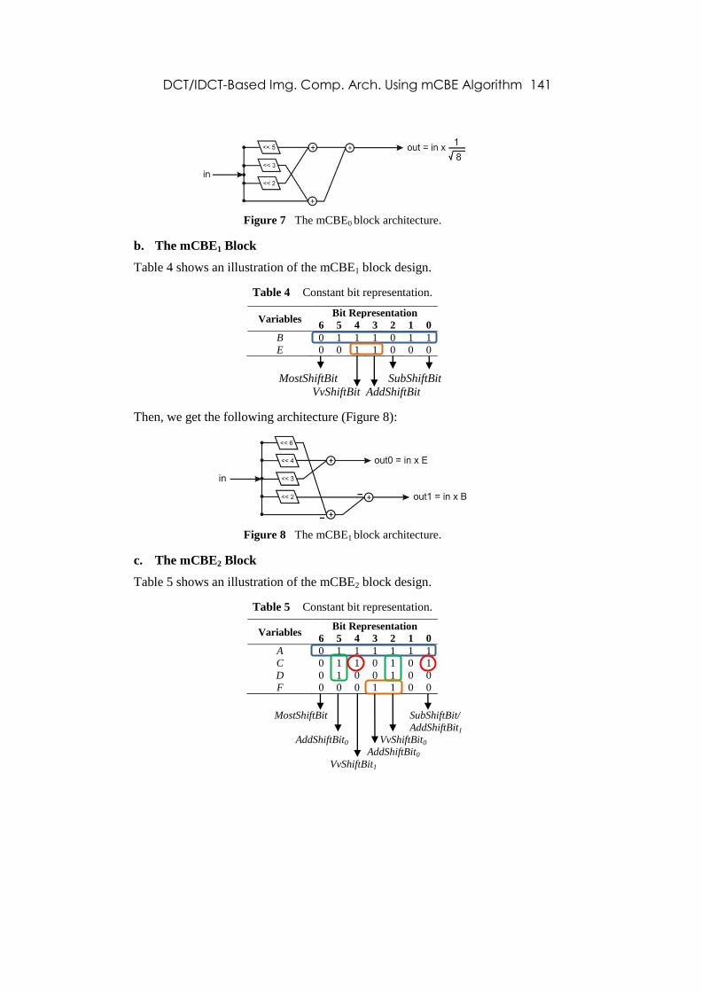
DCT/IDCT-Based Img. Comp. Arch. Using mCBE Algorithm 141
Figure 7 The mCBE0 block architecture.
b. The mCBE1 Block
Table 4 shows an illustration of the mCBE1 block design.
Table 4 Constant bit representation.
Variables Bit Representation
6 5 4 3 2 1 0
B 0 1 1 1 0 1 1
E 0 0 1 1 0 0 0
MostShiftBit SubShiftBit
VvShiftBit AddShiftBit
Then, we get the following architecture (Figure 8):
Figure 8 The mCBE1 block architecture.
c. The mCBE2 Block
Table 5 shows an illustration of the mCBE2 block design.
Table 5 Constant bit representation.
Variables Bit Representation
6 5 4 3 2 1 0
A 0 1 1 1 1 1 1
C 0 1 1 0 1 0 1
D 0 1 0 0 1 0 0
F 0 0 0 1 1 0 0
MostShiftBit SubShiftBit/
AddShiftBit1
AddShiftBit0 VvShiftBit0
AddShiftBit0
VvShiftBit1
142 Rachmad Vidya Wicaksana Putra, et. al.
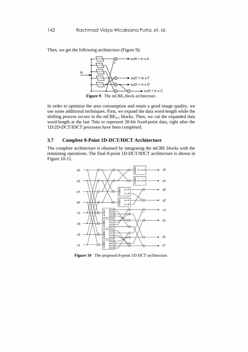
Then, we get the following architecture (Figure 9):
Figure 9 The mCBE2 block architecture.
In order to optimize the area consumption and retain a good image quality, we
use some additional techniques. First, we expand the data word-length while the
shifting process occurs in the mCBE0-2 blocks. Then, we cut the expanded data
word-length at the last 7bits to represent 20-bit fixed-point data, right after the
1D/2D-DCT/IDCT processes have been completed.
3.7 Complete 8-Point 1D-DCT/IDCT Architecture
The complete architecture is obtained by integrating the mCBE blocks with the
remaining operations. The final 8-point 1D-DCT/IDCT architecture is shown in
Figure 10-11.
Figure 10 The proposed 8-point 1D-DCT architecture.
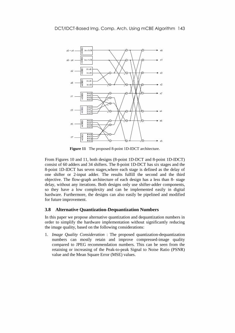
DCT/IDCT-Based Img. Comp. Arch. Using mCBE Algorithm 143
Figure 11 The proposed 8-point 1D-IDCT architecture.
From Figures 10 and 11, both designs (8-point 1D-DCT and 8-point 1D-IDCT)
consist of 60 adders and 34 shifters. The 8-point 1D-DCT has six stages and the
8-point 1D-IDCT has seven stages,where each stage is defined as the delay of
one shifter or 2-input adder. The results fulfill the second and the third
objective. The flow-graph architecture of each design has a less than 8- stage
delay, without any iterations. Both designs only use shifter-adder components,
so they have a low complexity and can be implemented easily in digital
hardware. Furthermore, the designs can also easily be pipelined and modified
for future improvement.
3.8 Alternative Quantization-Dequantization Numbers
In this paper we propose alternative quantization and dequantization numbers in
order to simplify the hardware implementation without significantly reducing
the image quality, based on the following considerations:
1. Image Quality Consideration : The proposed quantization-dequantization
numbers can mostly retain and improve compressed-image quality
compared to JPEG recommendation numbers. This can be seen from the
retaining or increasing of the Peak-to-peak Signal to Noise Ratio (PSNR)
value and the Mean Square Error (MSE) values.

144 Rachmad Vidya Wicaksana Putra, et. al.
2. Low Complexity Hardware Implementation : The proposed quantization-
dequantization numbers have to be implemented easily as shifter.
In order to retain image quality and get low complexity hardware, we adopt the
recommended quantization numbers as reference and change the value of the
numbers slightly compared to the recommended numbers, which are a power of
2.The proposed alternative quantization and dequantization numbers are:
128128128128128646464
12812812812864646432
1281281286464643232
128128646464323232
12864646432323216
6464643232321616
646432323216168
64323232161688
ECHROMINANCLUMINANCE QQ
For ease of reference, we call them FathQuantz numbers. If we use these
numbers, there are consequences that we need to know. The design can be
implemented easily as a shifter. However, the numbers are fixed, so we cannot
make them change dynamically in the digital hardware, except if we design a
supporting system for that case. In order to know the quality of the FathQuantz
numbers, we examined them and compared the results with the reference
numbers (JPEG recommendations, see Section 2.4). We use a comparison of
PSNR and MSE values to show in how far there is a difference between the
FathQuantz numbers and the reference numbers. The comparison results are
shown in Figures 12-13.
Figure 12 Comparison of PSNR values Figure 13 Comparison of MSE values.
In Figures 12 and 13, we can see that the PSNR and MSE values are not
significantly different between the reference and the FathQuantz numbers. The.
FathQuantz numbers can mostly retain the image quality compared to the
reference numbers. Therefore, we can use the FathQuantz numbers as
quantization-dequantization numbers.
DCT/IDCT-Based Img. Comp. Arch. Using mCBE Algorithm 145
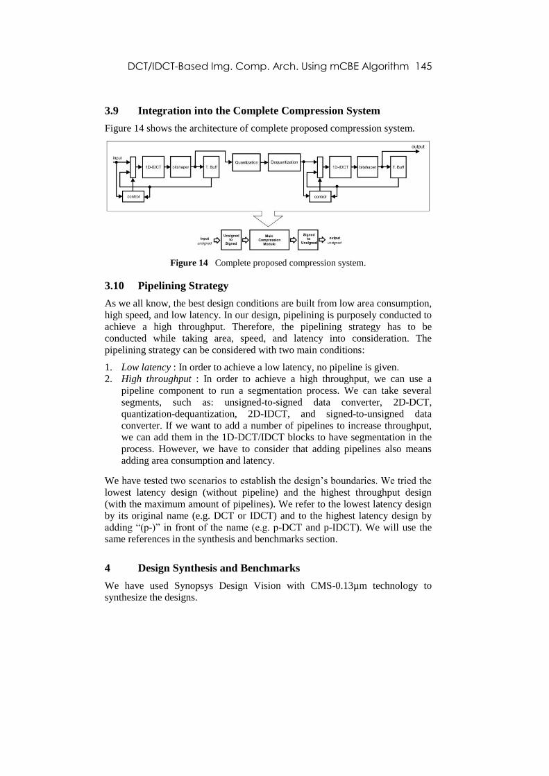
3.9 Integration into the Complete Compression System
Figure 14 shows the architecture of complete proposed compression system.
Figure 14 Complete proposed compression system.
3.10 Pipelining Strategy
As we all know, the best design conditions are built from low area consumption,
high speed, and low latency. In our design, pipelining is purposely conducted to
achieve a high throughput. Therefore, the pipelining strategy has to be
conducted while taking area, speed, and latency into consideration. The
pipelining strategy can be considered with two main conditions:
1. Low latency : In order to achieve a low latency, no pipeline is given.
2. High throughput : In order to achieve a high throughput, we can use a
pipeline component to run a segmentation process. We can take several
segments, such as: unsigned-to-signed data converter, 2D-DCT,
quantization-dequantization, 2D-IDCT, and signed-to-unsigned data
converter. If we want to add a number of pipelines to increase throughput,
we can add them in the 1D-DCT/IDCT blocks to have segmentation in the
process. However, we have to consider that adding pipelines also means
adding area consumption and latency.
We have tested two scenarios to establish the design’s boundaries. We tried the
lowest latency design (without pipeline) and the highest throughput design
(with the maximum amount of pipelines). We refer to the lowest latency design
by its original name (e.g. DCT or IDCT) and to the highest latency design by
adding “(p-)” in front of the name (e.g. p-DCT and p-IDCT). We will use the
same references in the synthesis and benchmarks section.
4 Design Synthesis and Benchmarks
We have used Synopsys Design Vision with CMS-0.13µm technology to
synthesize the designs.
146 Rachmad Vidya Wicaksana Putra, et. al.
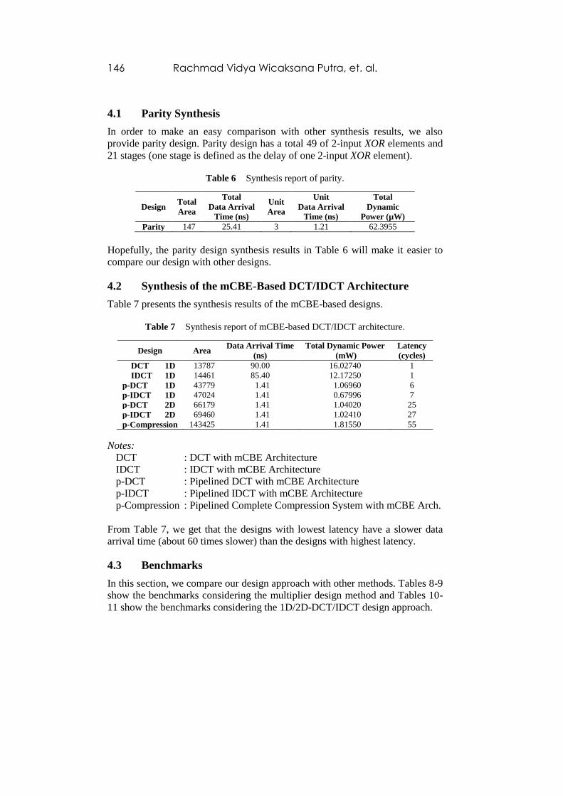
4.1 Parity Synthesis
In order to make an easy comparison with other synthesis results, we also
provide parity design. Parity design has a total 49 of 2-input XOR elements and
21 stages (one stage is defined as the delay of one 2-input XOR element).
Table 6 Synthesis report of parity.
Design Total
Area
Total
Data Arrival
Time (ns)
Unit
Area
Unit
Data Arrival
Time (ns)
Total
Dynamic
Power (µW)
Parity 147 25.41 3 1.21 62.3955
Hopefully, the parity design synthesis results in Table 6 will make it easier to
compare our design with other designs.
4.2 Synthesis of the mCBE-Based DCT/IDCT Architecture
Table 7 presents the synthesis results of the mCBE-based designs.
Table 7 Synthesis report of mCBE-based DCT/IDCT architecture.
Design Area Data Arrival Time
(ns)
Total Dynamic Power
(mW)
Latency
(cycles)
DCT 1D 13787 90.00 16.02740 1
IDCT 1D 14461 85.40 12.17250 1
p-DCT 1D 43779 1.41 1.06960 6
p-IDCT 1D 47024 1.41 0.67996 7
p-DCT 2D 66179 1.41 1.04020 25
p-IDCT 2D 69460 1.41 1.02410 27
p-Compression 143425 1.41 1.81550 55
Notes:
DCT : DCT with mCBE Architecture
IDCT : IDCT with mCBE Architecture
p-DCT : Pipelined DCT with mCBE Architecture
p-IDCT : Pipelined IDCT with mCBE Architecture
p-Compression : Pipelined Complete Compression System with mCBE Arch.
From Table 7, we get that the designs with lowest latency have a slower data
arrival time (about 60 times slower) than the designs with highest latency.
4.3 Benchmarks
In this section, we compare our design approach with other methods. Tables 8-9
show the benchmarks considering the multiplier design method and Tables 10-
11 show the benchmarks considering the 1D/2D-DCT/IDCT design approach.
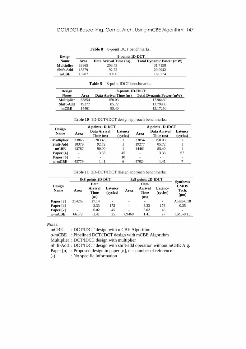
DCT/IDCT-Based Img. Comp. Arch. Using mCBE Algorithm 147
Table 8 8-point DCT benchmarks.
Design
Name
8-points 1D-DCT
Area Data Arrival Time (ns) Total Dynamic Power (mW)
Multiplier 33865 203.43 31.7158
Shift-Add 18379 92.72 20.0942
mCBE 13787 90.00 16.0274
Table 9 8-point IDCT benchmarks.
Design
Name
8-points 1D-IDCT
Area Data Arrival Time (ns) Total Dynamic Power (mW)
Multiplier 33854 150.03 17.96460
Shift-Add 19277 85.72 13.79980
mCBE 14461 85.40 12.17250
Table 10 1D-DCT/IDCT design approach benchmarks.
Design
Name
8-points 1D-DCT 8-points 1D-IDCT
Area Data Arrival
Time (ns)
Latency
(cycles) Area
Data Arrival
Time (ns)
Latency
(cycles)
Multiplier 33865 203.43 1 33854 150.03 1
Shift-Add 18379 92.72 1 19277 85.72 1
mCBE 13787 90.00 1 14461 85.40 1
Paper [4] - 3.33 45 - 3.33 67
Paper [6] - - 10 - - -
p-mCBE 43779 1.41 6 47024 1.41 7
Table 11 2D-DCT/IDCT design approach benchmarks.
Design
Name
8x8-points 2D-DCT 8x8-points 2D-IDCT Synthesis
CMOS
Tech.
(µm)
Area
Data
Arrival
Time
(ns)
Latency
(cycles) Area
Data
Arrival
Time
(ns)
Latency
(cycles)
Paper [3] 214263 17.14 - - - - Anam-0.18
Paper [4] - 3.33 172 - 3.33 178 0.35
Paper [7] - 6.02 45 - 6.02 45 -
p-mCBE 66179 1.41 25 69460 1.41 27 CMS-0.13
Notes:
mCBE : DCT/IDCT design with mCBE Algorithm
p-mCBE : Pipelined DCT/IDCT design with mCBE Algorithm
Multiplier : DCT/IDCT design with multiplier
Shift-Add : DCT/IDCT design with shift-add operation without mCBE Alg.
Paper [n] : Proposed design in paper [n], n = number of reference
(-) : No specific information
148 Rachmad Vidya Wicaksana Putra, et. al.
From Tables 8 and 9, the proposed design has a smaller area and a faster data
arrival time than the general multiplier method or the pure shift-add method.
Moreover, the DCT/IDCT designs with mCBE algorithm are almost three times
smaller and about two times faster than the multiplier-based architecture. The
proposed design is also smaller and faster than a pure shift-add architecture. In
Tables 10 and 11, we show the results of the comparison between the proposed
design and other proposed designs, such as the designs from references [6], [7],
[8] and [9]. The results show that our design can reach all three design
objectives (small area, multiplierless, and low complexity). Moreover, the
proposed design can achieve a high speed and relatively low latency compared
to the other designs.
5 Verification and Implementation
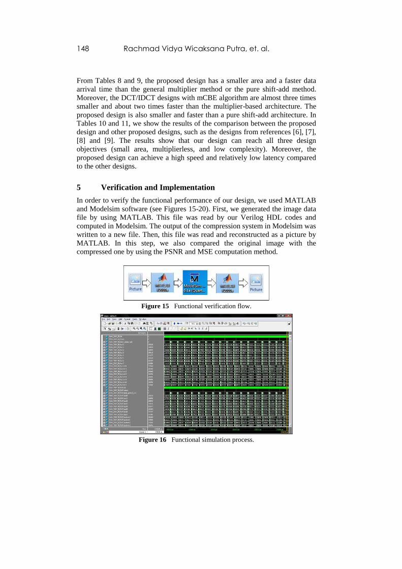
In order to verify the functional performance of our design, we used MATLAB
and Modelsim software (see Figures 15-20). First, we generated the image data
file by using MATLAB. This file was read by our Verilog HDL codes and
computed in Modelsim. The output of the compression system in Modelsim was
written to a new file. Then, this file was read and reconstructed as a picture by
MATLAB. In this step, we also compared the original image with the
compressed one by using the PSNR and MSE computation method.
Figure 15 Functional verification flow.
Figure 16 Functional simulation process.
DCT/IDCT-Based Img. Comp. Arch. Using mCBE Algorithm 149
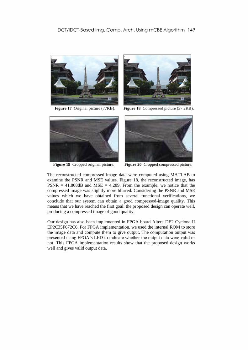
Figure 17 Original picture (77KB). Figure 18 Compressed picture (37.2KB).
Figure 19 Cropped original picture. Figure 20 Cropped compressed picture.
The reconstructed compressed image data were computed using MATLAB to
examine the PSNR and MSE values. Figure 18, the reconstructed image, has
PSNR = 41.808dB and MSE = 4.289. From the example, we notice that the
compressed image was slightly more blurred. Considering the PSNR and MSE
values which we have obtained from several functional verifications, we
conclude that our system can obtain a good compressed-image quality. This
means that we have reached the first goal: the proposed design can operate well,
producing a compressed image of good quality.
Our design has also been implemented in FPGA board Altera DE2 Cyclone II
EP2C35F672C6. For FPGA implementation, we used the internal ROM to store
the image data and compute them to give output. The computation output was
presented using FPGA’s LED to indicate whether the output data were valid or
not. This FPGA implementation results show that the proposed design works
well and gives valid output data.

150 Rachmad Vidya Wicaksana Putra, et. al.
6 Conclusion
We conclude that our design can reach all three objectives successfully. The
mCBE Algorithm can minimize the amount of shifter-adders to substitute
multipliers. Besides that, our alternative quantization-dequantization numbers
can mostly retain good compressed-image quality compared to JPEG
recommendations. The results of this research show that the proposed 8-point
1D-DCT design has only six stages and the 8-point 1D-IDCT design has only
seven stages. Here, we define one stage as equal to the delay of one shifter or 2-
input adder. By using the pipelining method, we can achieve a high-speed
architecture with latency as trade-off consideration. This design has been
synthesized and it can reach speeds of up to 1.41ns critical path delay
(709.22MHz).
References
[1] Salomon, D., Data Compression: The Complete Reference, 3rd Edition,
New York: Springer-Verlag, 2004.
[2] Loeffler, C., Lightenberg, A. & Moschytz, G.S., Practical Fast 1-D DCT
Algorithms with 11-Multiplications, Proceedings ICASSP, 1989.
[3] Jeong, H., Kim, J. & Cho, W.-k., Low-Power Multiplierless DCT
Architecture Using Image Data Correlation, IEEE Transactions on
Consumer Electronicsm, 2004.
[4] Ruiz, G.A., Michell, J.A. & Buron, A., High Throughput Parallel-
Pipeline 2-D DCT/IDCT Processor Chip, Journal of VLSI Signal
Processing, 45, pp. 161-175, 2006.
[5] Heyne, B. & Gotze, J., A Low Power and High Quality Implementation of
The Discrete Cosine Transformation, Advance in Radio Science, 2007.
[6] Kim, B.-I. & Ziavras, S.G., Low-Power Multiplierless DCT for
Image/Video Coders, IEEE 13th International Symposium on Consumer
Electronics, 2009.
[7] Subramanian, P. & Reddy, A.S.C., VLSI Implementation of Fully
Pipelined Multiplierless 2D DCT/IDCT Architecture for JPEG,
Proceedings ICSP, 2010.
[8] LSI Design Contest Official Website, Okinawa, Japan, http://lsi-
contest.com/2011/shiyou_3e.html (1 December 2010).
[9] Sung, T.Y., Shieh, Y.S. & Sun, M.J., A High-Throughput and Memory-
Efficiency 2D DCT Architecture based on Cordic Rotation, The 23rd
Workshop on Combinatorial Mathematics and Computation Theory.
Related Documents