A new, practical approach to maintaining an efficient yet acceptably-performing wireless networked control system

A New, Practical Approach to Maintaining an Efficient YetAcceptably-performing Wireless Networked Control System

James H. Taylor� and Hazem M. S. Ibrahim†

Dep’t. of Electrical & Computer EngineeringUniversity of New Brunswick

Fredericton, N.B., CANADA E3B 5A3�jim [email protected] ; †[email protected]

Abstract— Wireless networked control systems have begun togain acceptance during the last decade, due to the increasedflexibility and lower costs they promise to provide compared withwired installations. The pace of application has been held back,however, by the reluctance of industry to make the accommoda-tions necessary to allow wireless paths to be incorporated safelyin process control loops, thus limiting the potential applicationsand benefits of wireless systems. Wireless control signals face timedelay that may degrade the performance of the control loop oreven lead to instability. This time delay depends on the networkconfiguration. The sampling rate also has a great impact onthe stability and performance of the closed-loop control systemover the communication networks, yet the data rate should beminimized to conserve node battery life.

The main goal of this paper is to present and discuss areal-time nonlinear control system approach that (1) checks aproposed network configuration to determine the time delaywhich the control data packets will encounter, and rejectany proposed configuration that would lead to poor closed-loop system performance; and (2) determines the minimumacceptable sampled data rate that does not degrade control loopperformance excessively. The jacketed continuous stirred-tankreactor will be presented as a typical application, to illustrateand validate this development.

Keywords — wireless sensor networks, wireless control loops,WSN energy conservation, control loop performance

I. INTRODUCTION

During the past two decades, a large amount of research hasbeen done on distributed control systems that incorporate wire-less sensor networks, or what are called Wireless NetworkedControl Systems (WNCSs). That interest can be traced to themany advantages achieved by eliminating the costs and restric-tions of traditional point-to-point wired control architectures,such as a reduction in wiring cost, rapid deployment, flexibleinstallation, fully mobile operation, and improved freedom inplacement of controllers [1] [2] [3] [4] [5]. In such systems,distributed sensors, controllers, and actuators are exchanginginformation over a wireless communication network.

Improved technology and stricter requirements make thedevelopment of WNCSs more difficult, however. Part of theproblem arises from inflexibility in the imposition of strictrequirements on data rates, latency and data loss to ensurecontrol system performance on one hand [3] [5], and effectiveprotocols for wireless sensor network (WSN) robustness andefficiency on the other [1] [4]. Our primary interest in WNCSsis for Petroleum Applications of Wireless Systems (PAWS1), amajor research program at Cape Breton University (CBU, the

1The Petroleum Applications of Wireless Systems project is supported bythe Government of Canada, through the Atlantic Innovation Fund (AIF).

project lead organization that deals with WSNs [5] [6]) and theUniversity of New Brunswick (UNB, focussed on IntelligentControl and Asset Management or ICAM [7]).

WSN data rates affect both the performance of a controlsystem implemented with wireless communication links in itsclosed loops and the WSN nodes’ energy consumption. Themain goal of this paper is to present a pragmatic way todetermine the minimum data rates (maximum sampling timesτs−max) that maintain adequate performance of the closed loopcontrol system, thus allowing the energy consumption of theWSN nodes to be reduced to the extent possible.

As is well known, the value of τs−max depends on the datadelays or latencies τd introduced in the control loop paths bythe WSN; this, in turn, depends on the WSN configuration,especially the number of hops in these paths. If we accountfor delay via a conservative (worst-case) design, based, forexample, on the maximum number of hops and the maximumdelay per hop, then an unreasonably small τs−max may bedemanded; this we wish to avoid. Therefore, we assume that τd

can be determined experimentally for the WSN configuration inuse, by using either time stamps, ‘ping’ tests or counting hops.WSN reconfiguration will obviously require a redeterminationof τd and τs−min(τd), so the approach should be relativelyeasy to execute and fast.

The UNB team has developed a Wireless Networked ControlSystem Coordination Agent (WNCSCA), which is responsiblefor assigning and managing the WSN data rates as well asaccepting or rejecting the configuration of the WSN based ondelays in the control-loop paths over the WSN. Both of thesefactors have a major impact on controller performance, andthe WNCSCA will not only maintain the stability of the closed-loop control system but also guard against the performance ofthe closed loop control system degrading excessively. On theother hand, node energy conservation is a critical issue in WSNsin terms of node and network life, as the nodes are usuallypowered by batteries, and in many cases the replacement ofthese power sources is difficult, inconvenient, and/or expensive.Our WNCSCA coordinates with ICAM and the WSN Gateway toallow as much network optimization and flexibility as possibleunder constraints imposed by the WNCS requirements.

II. WNCS COORDINATION AGENT

Our WNCSCA is being implemented as a part of ICAM,which is a multi-agent intelligent supervisory system forpetroleum processing facilities [7]. This agent will medi-ate between the ICAM system and the Gateway of CBU’sWireless Industrial Sensor Network Testbed For Radio-Harsh

978-1-4244-6474-6/10/$26.00 ©2010 IEEE ICSSE 2010 in Taiwan

Environments (WINTeR), which is an open-access, multi-userexperimental testbed, developed under the PAWS project, tosupport implementation and evaluation of WSNs for industrialapplications [6]. WINTeR now supports process simulationswith wireless in the loop; in the future the goal is to interfaceWINTeR with actual industrial processes as well. There aretwo process simulators currently linked to WINTeR, one ahigh-order, highly complex model of a three-phase crude-oilseparator [8] which has five control loops, and the other asimpler model of a jacketed continuous stirred-tank reactor(JCSTR) [9]. The JCSTR has been chosen and implemented asa process simulator to better allow the study of issues relatedto the stability and performance of control systems over aWSN; this will facilitate development of the WNCSCA, thusforming an important enabling technology for the use of WSNsin process control applications.

During the operation of the ICAM system, its controllersand agents may require different levels of service from theWSN to complete their functions properly. These agents includeFault Detection, Isolation and Accommodation (FDIA) [11],Nonlinear Dynamic Data Reconciliation (NDDR) [12], Lin-earized Model Identification (LMId) [13] and other subsidiaryfunctions. For example, the controllers require different datarates from specific sensors and actuators in specific regimes,such as start-up, set point changes and steady state operation.During start-up and set point changes, the process variabletransients must decay properly under closed-loop control, soappropriate data rates and path delays must be imposed. Oncethe process reaches the desired steady-state set-point the LMIdagent perturbs the plant with pseudo-random signals (to exciteall the modes in the plant), gather data and apply its modelidentification algorithm, perhaps needing a different data ratethan before. After that, the process may remain settled insteady state, in which case loops can be opened2 and data ratessubstantially reduced so ICAM can monitor the process; as longas there are no disturbances or set-point changes slow samplingcan continue and the WSN Gateway can manage its operationsfreely and conserve energy accordingly. Alternatively, if FDIAis to continue during steady state (and that would most likely bedesirable) data rates can be reduced somewhat, but not as muchas passive monitoring would allow. In many industrial systemsa process may be in steady state for long periods of time, withinfrequent set-point changes requiring closed-loop control, sothis strategy will allow the WSN to be managed in a moreenergy-efficient manner much of the time. A communicationprotocol for the WNCSCA is developed and presented in [14];in this paper we focus on issues relating to the managementof time delay and sampling rate.

In summary, the various modes of operation require tighteror looser constraints on data rates and control signal pathdelays; the WNCSCA mediates between ICAM and the WSNGateway to allow both the control system and the WSN tomeet their objectives as flexibly and effectively as possible.

III. JCSTR PROCESS SIMULATION MODEL

The ICAM system processes real-time data that are collectedfrom either an external plant or from a real-time processsimulation model which reproduces the nonlinear nature ofa typical petroleum application plant. UNB’s real-time JCSTRsimulator is embedded in WINTeR at Cape Breton University

2Opening control loops momentarily to handle data drop-outs has beensuggested in [3]; we believe that our strategy of opening control loops duringsteady-state operation to remove strict control-related WSN constraints is new.

to permit running experiments with wireless-in-the-loop. Thephysical characteristics, modeling and simulation of the JCSTRare outlined in the following sections.

A. Nonlinear JCSTR simulator

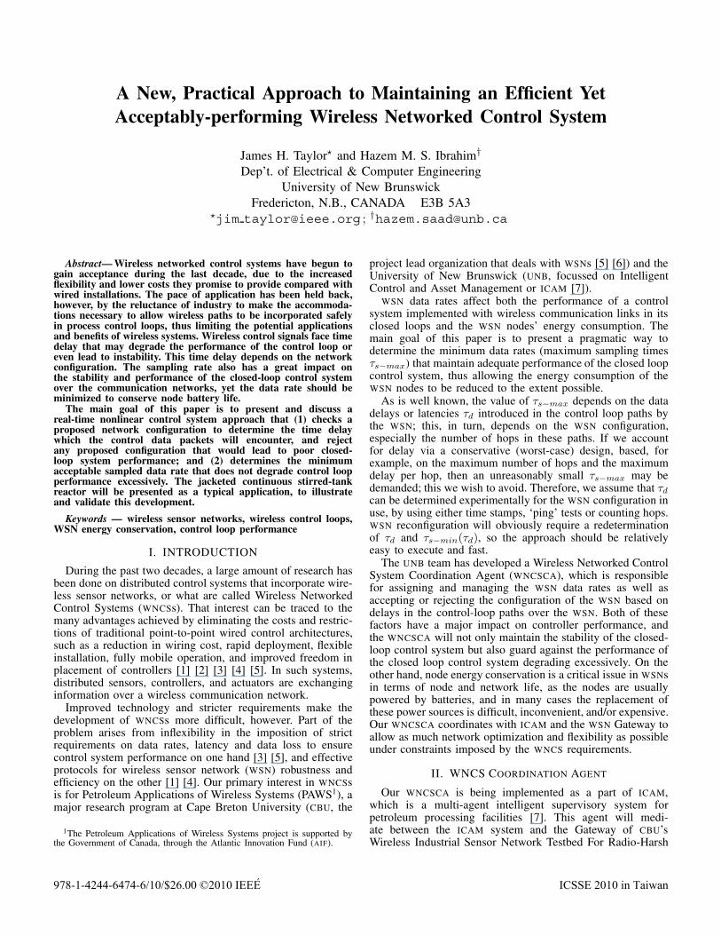
The JCSTR simulator was implemented as both a MATLAB R©function [9] (encoding the vector differential equations forthe nonlinear JCSTR including the PI controller, suitable foruse with MATLAB R© integrators such as ode45) and as aSimulink R© model (with the physical process modeled asMATLAB R© code in an S function, digital controller blocks,delay elements and zero-order holds). A schematic of theJCSTR is depicted in figure 1. As shown, the tank inlet or“mixture” flow is received from another process unit. There isalso a heating fluid circulated through the jacket in order to heatthe mixture inside the tank. The main objective of the JCSTRis to control the mixture level (via the level controller or LC)and the mixture temperature (via the temperature controller orTC) inside the tank reactor. This is done by controlling thejacket inlet valve flow rate and the tank outlet valve flow rate.

The following assumptions were made in order to derive thedynamic modeling equations of the tank and jacket:

• Liquids have constant density and heat capacity.

• Mixing in both the tank and the jacket is ideal.

• The amount of liquid in the jacket is constant, i.e., Fjin =Fjout.

• The tank inlet flow rate, tank inlet temperature and jacketinlet temperature may change; these are uncontrolledinputs.

• The tank outlet flow rate and jacket flow rate are controlinputs (actuation).

• The rate of heat transfer from the jacket to the tankis governed by Q = U AH (Tj − T ), where U is theoverall heat transfer coefficient and AH is the area forheat transfer, AH = AB + πDH where AB is the areaof the base, D is the diameter of the base and H is theheight of the mixture.

Fig. 1. Jacketed continuously stirred-tank reactor.

The JCSTR process is described by a third-order model whichhas two control inputs, three state variables, and two controlledvariables. Specifically, the state variables are mixture height,H , mixture temperature, T , and the jacket temperature, Tj ;x = [ H T Tj ]T . The input variables are divided into two

ICSSE 2010 in Taiwan

groups: control inputs, i.e., mixture outflow, Fout, and jacketinflow, Fjin; u = [ Fout Fjin ]T ; and exogenous inputs, viz.mixture inflow, Fin, temperature of the mixture feed, Tin, andtemperature of the jacket inflow, Tjin; w = [ Fin Tin Tjin ]T .Finally, the JCSTR outputs are the controlled variables H andT ; y = [ H T ]T = [ x1 x2 ]T . The exogenous inputs may beregarded as disturbances; here we consider them to be constant.

The following ordinary differential equations describe thedynamic behavior of the JCSTR:

H =1

AB(Fin − Fout)

T =Fin(Tin − T )

ABH+

UAH(Tj − T )ρ CpABH

(1)

Tj =Fjin(Tjin − Tj)

Vj− UAH(Tj − T )

ρ CpVj

where the subscripts in, out, j refer to inlet, outlet and jacketrespectively. In addition to the parameters defined above, wehave ρ = mixture density, Cp = heat capacity of the mixtureand Vj = jacket water volume. The values of the JCSTR modelparameters are provided in [9]. Note that the size of the unithas a major impact on the system time constants; here we usenormalized units for level and time, i.e., both variables aregiven in per unit (pu) rather than meters and minutes.

B. Controller design for the JCSTRLinearization about the set point has been used in order to

design a controller for this nonlinear system. Most processcontrol systems are required to keep the states of the dy-namic process at specific constant values or set points. Thisis achieved by providing control signals (plant inputs) thathave two components: The first part or feedforward termu generates the control signal needed to keep the process atthe set point in steady state, and the second component orfeedback term δu generates the incremental control neededto return the process to the set point if it should deviate fromit [10]. The structure of the control system designed in thisway is shown in figure 2.

−

.δ

.

Set Point

Controller Plant

_

_

_ ++ x = f(x,u)

y = h(x,u)Ce y+y

u( )

u

u u

Fig. 2. Control system structure, linearization about a set point.

The steady-state control component can be determined asfollows: Given a nonlinear process,

x = f(x, u) , y = g(x, u) (2)

Suppose that y is the set point or desired output for the controlsystem, which is assumed to be constant. Suppose also thatx and u are the steady-state values of the state and control,respectively, that produce this constant output. Since x is thusan equilibrium state we have x = 0, so we have to solve a setof algebraic equations,

0 = f(x, u) , y = g(x, u) (3)

For the JCSTR we have y = [ x1 x2 ]T with given set-pointvalues, and x3, u1 and u2 as unknowns, so this is a well-posedproblem involving the solution of three simultaneous equations(f(x, u) = 0) in three unknowns.

The feedback controller operates on the error or differencebetween the desired output y and the actual output y to generatea corrective control signal δu. Then, the corrective controlsignal is summed with the feedforward control signal u toproduce the actual control signal u as input to the plant.

Substituting the previous definitions of x and u into eqns.(1) we can write the three state differential equations as:

x1 =1

AB(Fin − u1)

x2 =Fin(Tin − x2)

ABx1+

U(x3 − x2)ρ Cp x1

+UπD(x3 − x2)

ρ CpAB(4)

x3 =u2(Tjin − x3)

Vj− UAB(x3 − x2)

ρ Cp Vj− UπDx1(x3 − x2)

ρ Cp Vj

Therefore, the equilibrium conditions using eqn. (3) are:

u1 = Fin

u2 =Fin(x2 − Tin)

Tjin − x3

x1 = y1 = set point 1 (given) (5)x2 = y2 = set point 2 (given)

x3 = x2 +FinρCp(x2 − Tin)UAB + UπDx1

The second and fifth relations can be solved to obtain

x3 = x2 +Fin (x2 − Tin)

α (AB + πDrx1)(6)

u2 =Fin (x2 − Tin)

Tjin − x3(7)

As mentioned, we used small signal linearization to designthe feedback controller C which regulates the system tomaintain its output at the desired set point. This procedureis well known, so we merely refer to [9] for the (A, B, C, D)array elements in the usual linearized model formulation.

We converted the linearized state space formulation to itsequivalent transfer function form, and designed a suitablediagonal 2 × 2 PI controller that gives a fast response withmoderate overshoot.

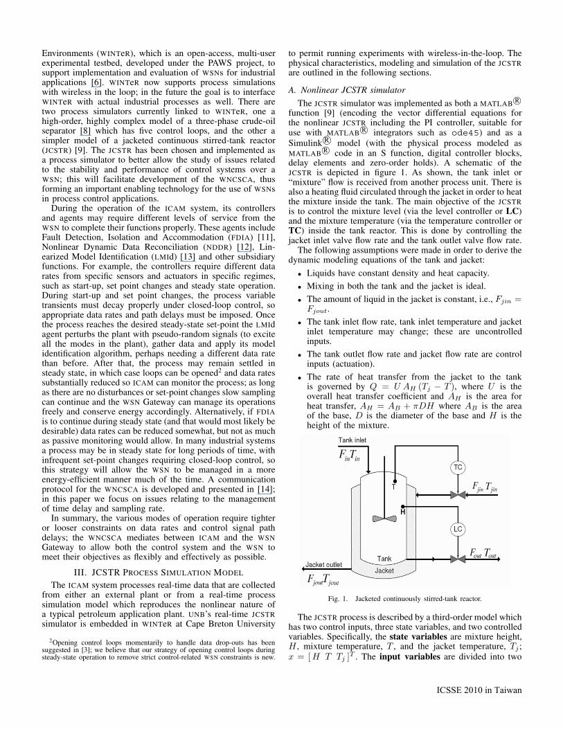
C. JCSTR simulator benchmarkIn order to establish the process simulator’s ideal perfor-

mance under digital control, with no delay and fast samplingtime τs = 0.1 pu, step changes are applied to the set pointsfor the level and the temperature of the mixture inside the tankreactor. Specifically, we start with the initial conditions of thestates being x10 = 0.66 pu, x20 = 50 C, and x30 = 143 C,and apply two successive set-point changes for the level andthe temperature inside the reactor. The level set point changesat t = 1.8 pu from 0.7 pu to 0.75 pu. The mixture temperatureset point changes at t = 2.4 pu from 52 C to 56 C. The stepresponses of these changes in the set points are shown in figures3 and 4, respectively. The corresponding benchmark percentovershoots (% OSs) are 10.8 for the level loop and 11.0 for themixture temperature loop.

Changing the sampling time: The sampling time τs−LC

of the mixture level sensor was varied to check its effect

ICSSE 2010 in Taiwan

0 1 2 3 4 50.64

0.66

0.68

0.7

0.72

0.74

0.76

Nor

mal

ized

Lev

el (

pu)

Normalized Time (pu)

Mixture Level

Fig. 3. Mixture level vs normalized time.

0 1 2 3 4 550

51

52

53

54

55

56

57

Normalized Time (pu)

Mixture Temperature

Mix

tem

p. (

Deg

rees

C)

Fig. 4. Mixture temperature vs normalized time.

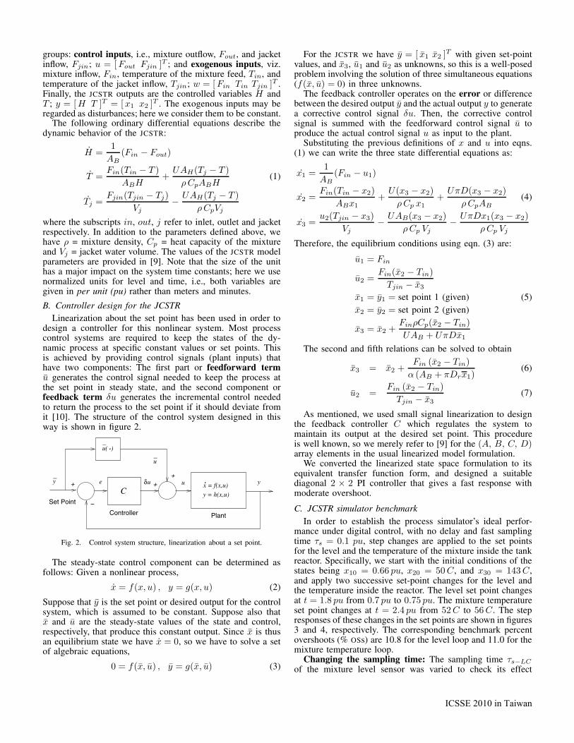
on closed loop control performance. Note that we do notmerely insist on stability, we establish a threshold of accept-able percent overshoot, here taken to be 25%. By iterativelyadjusting τs−LC , we found that the minimum sampling ratethat keeps the mixture level control performance acceptable inthis sense is 0.25 pu, which gives 24.9 % OS, as shown infigure 5. Of course, more conservative values of % OS can bemandated, e.g., benchmark % OS = 0, maximum acceptable% OS = 10. The same method was applied to the mixture

0 1 2 3 4 50.64

0.66

0.68

0.7

0.72

0.74

0.76

0.78

Normalized Time (pu)

Nor

mal

ized

Lev

el (

pu)

Mixture Level

Fig. 5. Mixture level vs normalized time, τs−LC = 0.25 pu (24.9% OS).

0 1 2 3 4 550

51

52

53

54

55

56

57

58

Normalized Time (pu)

Mix

tem

p. (

Deg

rees

C)

Mixture Temperature

Fig. 6. Mixture temperature vs normalized time, τs−TC = 0.3 pu (28.5%OS).

temperature control loop. By changing the sampling time forthe mixture temperature sensor, τs−TC , we found that themaximum sampling rate that produces acceptable % OS is 0.3pu, which yielded 28.5% OS, as shown in figure 6.

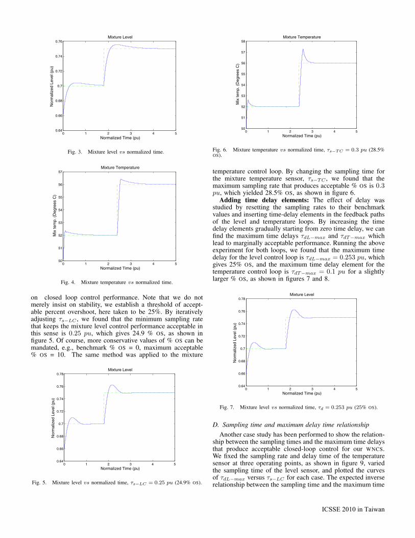
Adding time delay elements: The effect of delay wasstudied by resetting the sampling rates to their benchmarkvalues and inserting time-delay elements in the feedback pathsof the level and temperature loops. By increasing the timedelay elements gradually starting from zero time delay, we canfind the maximum time delays τdL−max and τdT−max whichlead to marginally acceptable performance. Running the aboveexperiment for both loops, we found that the maximum timedelay for the level control loop is τdL−max = 0.253 pu, whichgives 25% OS, and the maximum time delay element for thetemperature control loop is τdT−max = 0.1 pu for a slightlylarger % OS, as shown in figures 7 and 8.

0 1 2 3 4 50.64

0.66

0.68

0.7

0.72

0.74

0.76

0.78

Normalized Time (pu)

Nor

mal

ized

Lev

el (

pu)

Mixture Level

Fig. 7. Mixture level vs normalized time, τd = 0.253 pu (25% OS).

D. Sampling time and maximum delay time relationship

Another case study has been performed to show the relation-ship between the sampling times and the maximum time delaysthat produce acceptable closed-loop control for our WNCS.We fixed the sampling rate and delay time of the temperaturesensor at three operating points, as shown in figure 9, variedthe sampling time of the level sensor, and plotted the curvesof τdL−max versus τs−LC for each case. The expected inverserelationship between the sampling time and the maximum time

ICSSE 2010 in Taiwan

delay for % OS ≤ 25 has been determined, as shown in thatfigure. These plots also reveal the interactive nature of thesetwo loops.

This study was also reversed, by fixing the sampling rate anddelay time of the level sensor at three operating points, varyingthe sampling time of the temperature sensor, and plotting thecurves of τdT−max versus τs−TC for each case; here, too, weobserved a similar relationship and interaction between the twoloops.

0 1 2 3 4 550

51

52

53

54

55

56

57

58

Mix

tem

p. (

Deg

rees

C)

Mixture Temperature

Normalized Time (pu)

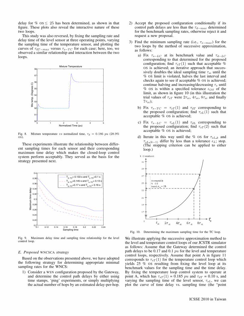
Fig. 8. Mixture temperature vs normalized time, τd = 0.186 pu (28.9%OS).

These experiments illustrate the relationship between differ-ent sampling times for each sensor and their correspondingmaximum time delay which makes the closed-loop controlsystem perform acceptably. They served as the basis for thestrategy presented next.

0.1 0.12 0.14 0.16 0.18 0.2 0.22 0.240.2

0.22

0.24

0.26

0.28

0.3

0.32

0.34

0.36

0.38

0.4

Sampling time

Max

imum

tim

e de

lay

Td−TC= 0.133 s and Ts−TC=0.1 s

Td−TC=0.145 s and Ts−TC= 0.13 s

Td−TC=0.17 s and Ts−TC= 0.16 s

Fig. 9. Maximum delay time and sampling time relationship for the levelcontrol loop.

E. Proposed WNCSCA strategy

Based on the observations presented above, we have adoptedthe following strategy for determining appropriate minimalsampling rates for the WNCS:

1) Consider a WSN configuration proposed by the Gateway,and determine the control path delays by either usingtime stamps, ‘ping’ experiments, or simply multiplyingthe actual number of hops by an estimated delay-per-hop.

2) Accept the proposed configuration conditionally if itscontrol path delays are less than the τd−max determinedfor the benchmark sampling rates, otherwise reject it andrequest a new proposal.

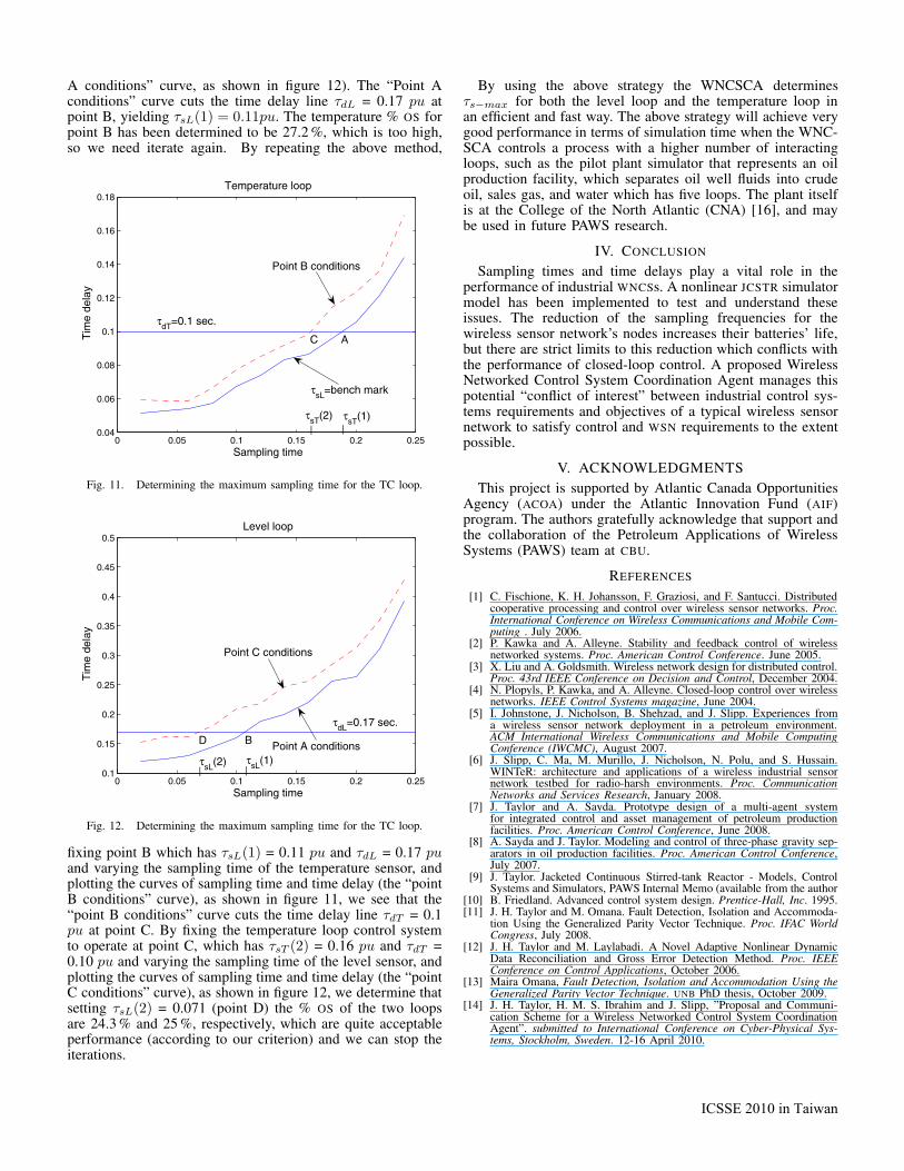
3) Find the minimum sampling rate (i.e., τs−max) for thetwo loops by the method of successive approximation,as follows:

a) Fix τs−LC at its benchmark value and τd−LC

corresponding to that determined for the proposedconfiguration; find τsT (1) such that acceptable %OS is achieved; an iterative approach that succes-sively doubles the ideal sampling time τsi until the% OS limit is violated, halves the last interval andchecks again to see if acceptable % OS is achieved;continue halving and increasing/decreasing τs until% OS is within a specified tolerance εOS of thelimit, as shown in figure 10 (in this illustration thetrial values of τsT were 2τsi, 4τsi, 8τsi and finally7τsi);

b) Fix τs−TC = τsT (1) and τdT corresponding tothe proposed configuration; find τsL(1) such thatacceptable % OS is achieved;

c) Fix τs−LC = τsL(1) and τdL corresponding tothe proposed configuration; find τsT (2) such thatacceptable % OS is achieved;

d) Iterate in this way until the % OS for τsL k andτsL (k−1) differ by less than a tolerance εL; stop.(The stopping criterion can be applied to eitherloop.)

31

19

21

23

25

27

29

17

ssi si2 si4 si6 si8

% Overshoot

~~0

Acceptable% OSband, %2so

Fig. 10. Determining the maximum sampling time for the TC loop.

We illustrate applying the successive approximation method tothe level and temperature control loops of our JCSTR simulatoras follows: Assume that the Gateway determined the controlpath delays to be 0.17 and 0.1 pu for the level and temperaturecontrol loops, respectively. Assume that point A in figure 11corresponds to τsT (1) for the temperature control loop whichyields 25 % OS resulting from fixing the level loop at itsbenchmark values for the sampling time and the time delay.By fixing the temperature loop control system to operate atpoint A, which has τsT (1) = 0.185 pu and τdT = 0.10 s, andvarying the sampling time of the level sensor, τsL, we canplot the curve of time delay vs. sampling time (the “point

ICSSE 2010 in Taiwan

A conditions” curve, as shown in figure 12). The “Point Aconditions” curve cuts the time delay line τdL = 0.17 pu atpoint B, yielding τsL(1) = 0.11pu. The temperature % OS forpoint B has been determined to be 27.2 %, which is too high,so we need iterate again. By repeating the above method,

0 0.05 0.1 0.15 0.2 0.250.04

0.06

0.08

0.1

0.12

0.14

0.16

0.18

Sampling time

Tim

e de

lay

Temperature loop

AC

τdT=0.1 sec.

||τsT(1)τsT(2)

τsL=bench mark

Point B conditions

Fig. 11. Determining the maximum sampling time for the TC loop.

0 0.05 0.1 0.15 0.2 0.250.1

0.15

0.2

0.25

0.3

0.35

0.4

0.45

0.5

Sampling time

Tim

e de

lay

Level loop

BD

τdL=0.17 sec.

||τsL(1)τsL(2)

Point C conditions

Point A conditions

Fig. 12. Determining the maximum sampling time for the TC loop.

fixing point B which has τsL(1) = 0.11 pu and τdL = 0.17 puand varying the sampling time of the temperature sensor, andplotting the curves of sampling time and time delay (the “pointB conditions” curve), as shown in figure 11, we see that the“point B conditions” curve cuts the time delay line τdT = 0.1pu at point C. By fixing the temperature loop control systemto operate at point C, which has τsT (2) = 0.16 pu and τdT =0.10 pu and varying the sampling time of the level sensor, andplotting the curves of sampling time and time delay (the “pointC conditions” curve), as shown in figure 12, we determine thatsetting τsL(2) = 0.071 (point D) the % OS of the two loopsare 24.3 % and 25 %, respectively, which are quite acceptableperformance (according to our criterion) and we can stop theiterations.

By using the above strategy the WNCSCA determinesτs−max for both the level loop and the temperature loop inan efficient and fast way. The above strategy will achieve verygood performance in terms of simulation time when the WNC-SCA controls a process with a higher number of interactingloops, such as the pilot plant simulator that represents an oilproduction facility, which separates oil well fluids into crudeoil, sales gas, and water which has five loops. The plant itselfis at the College of the North Atlantic (CNA) [16], and maybe used in future PAWS research.

IV. CONCLUSION

Sampling times and time delays play a vital role in theperformance of industrial WNCSs. A nonlinear JCSTR simulatormodel has been implemented to test and understand theseissues. The reduction of the sampling frequencies for thewireless sensor network’s nodes increases their batteries’ life,but there are strict limits to this reduction which conflicts withthe performance of closed-loop control. A proposed WirelessNetworked Control System Coordination Agent manages thispotential “conflict of interest” between industrial control sys-tems requirements and objectives of a typical wireless sensornetwork to satisfy control and WSN requirements to the extentpossible.

V. ACKNOWLEDGMENTSThis project is supported by Atlantic Canada Opportunities

Agency (ACOA) under the Atlantic Innovation Fund (AIF)program. The authors gratefully acknowledge that support andthe collaboration of the Petroleum Applications of WirelessSystems (PAWS) team at CBU.

REFERENCES

[1] C. Fischione, K. H. Johansson, F. Graziosi, and F. Santucci. Distributedcooperative processing and control over wireless sensor networks. Proc.International Conference on Wireless Communications and Mobile Com-puting . July 2006.

[2] P. Kawka and A. Alleyne. Stability and feedback control of wirelessnetworked systems. Proc. American Control Conference. June 2005.

[3] X. Liu and A. Goldsmith. Wireless network design for distributed control.Proc. 43rd IEEE Conference on Decision and Control, December 2004.

[4] N. Plopyls, P. Kawka, and A. Alleyne. Closed-loop control over wirelessnetworks. IEEE Control Systems magazine, June 2004.

[5] I. Johnstone, J. Nicholson, B. Shehzad, and J. Slipp. Experiences froma wireless sensor network deployment in a petroleum environment.ACM International Wireless Communications and Mobile ComputingConference (IWCMC), August 2007.

[6] J. Slipp, C. Ma, M. Murillo, J. Nicholson, N. Polu, and S. Hussain.WINTeR: architecture and applications of a wireless industrial sensornetwork testbed for radio-harsh environments. Proc. CommunicationNetworks and Services Research, January 2008.

[7] J. Taylor and A. Sayda. Prototype design of a multi-agent systemfor integrated control and asset management of petroleum productionfacilities. Proc. American Control Conference, June 2008.

[8] A. Sayda and J. Taylor. Modeling and control of three-phase gravity sep-arators in oil production facilities. Proc. American Control Conference,July 2007.

[9] J. Taylor. Jacketed Continuous Stirred-tank Reactor - Models, ControlSystems and Simulators, PAWS Internal Memo (available from the author

[10] B. Friedland. Advanced control system design. Prentice-Hall, Inc. 1995.[11] J. H. Taylor and M. Omana. Fault Detection, Isolation and Accommoda-

tion Using the Generalized Parity Vector Technique. Proc. IFAC WorldCongress, July 2008.

[12] J. H. Taylor and M. Laylabadi. A Novel Adaptive Nonlinear DynamicData Reconciliation and Gross Error Detection Method. Proc. IEEEConference on Control Applications, October 2006.

[13] Maira Omana, Fault Detection, Isolation and Accommodation Using theGeneralized Parity Vector Technique. UNB PhD thesis, October 2009.

[14] J. H. Taylor, H. M. S. Ibrahim and J. Slipp, ”Proposal and Communi-cation Scheme for a Wireless Networked Control System CoordinationAgent”. submitted to International Conference on Cyber-Physical Sys-tems, Stockholm, Sweden. 12-16 April 2010.

ICSSE 2010 in Taiwan