A New Optimization Model for Designing Acceptance …

67

A New Optimization Model for Designing Acceptance Sampling Plan Based on Run Length of Conforming Items

Mohammad Saber Fallahnezhad1*, ahmad Ahmadi Yazdi2 1Departement of Industrial Engineering, Yazd university, Yazd, Iran

2Isfahan University of Technology, Isfahan, Iran [email protected], [email protected]

Abstract

The purpose of this article is to present an optimization model for designing an acceptance sampling plan based on cumulative sum of run length of conforming items. The objective is to minimize the total loss including both the producer and consumer losses. The concept of minimum angle method is applied to consider producer and consumer risks in the optimization model. Also the average number of inspection is considered in the constraint of the model. A practical case study has been done and a sensitivity analysis is performed for elaborating the effect of some important parameters on the objective function. The results of sensitivity analysis showed that the performance of the proposed model is logical, reliable in all the cases and also has better performance in comparison with classical method in most of the cases. A computational experiment is done to compare the different sampling schemes. The results of computational experiment showed that the proposed model has better performance due to smaller ANI value in all cases. Keywords: Quality control, Conforming run length, Acceptance Sampling Plan, Minimum angle method, Taguchi loss function

1- Introduction

The purpose of this paper is to design an optimization model to determine the optimal sampling plan which minimizes the producer’s loss plus the consumer’s quality loss while considering the average sample number along with the producer’s and consumer’s risks. Acceptance sampling is a branch of quality control which provides decision rules for producers and consumers to make a decision about a lot of items. Different methods are available for designing economic acceptance sampling methods. The proposed model is developed to consider some key concepts in production environments. The first important concept is related to quality cost. Quality cost has two parts. One part is the cost of unsatisfied consumer which is the result of the deviation of quality characteristic from its target value which is known as the consumer loss. The second part is the quality cost for producer. It is obvious that rejecting an item has cost for producer which includes the cost of processing and reprocessing the item.

*Corresponding author. ISSN: 1735-8272, Copyright c 2016 JISE. All rights reserved

Journal of Industrial and Systems Engineering Vol. 9, No. 2, pp 67-87 Spring (April) 2016

68

Also inspecting the items has cost because of applying inspection equipment or employing inspectors. It is obvious that total inspection cost is a function of average number of conforming items that is abbreviated as ANI. Along with optimizing quantitative measures of sampling method, some qualitative properties of sampling plan should be optimized simultaneously. Most important criterion for a sampling system is the risk to producer and the risk to consumer. These two risks can be considered in one objective function as performed in minimum angle method (Fallahnezhad, 2012). Thus we tried to develop a general optimization model which considers all these important criteria in one model. Thus all objectives are optimized simultaneously in contrast with previous models where usually only one or two of these objectives have been optimized together. It is clear that we may improve the performance of sampling system in any production environments by taking all important aspects of sampling plan into account. Ferrell and Chhoker (2002) presented an economical acceptance sampling plan. Their plan has 3 options: (1) they used continuous loss function. (2) Inspection error is considered in their sampling plan. (3) Their model can be used for designing near optimal sampling plan. They constructed graphs in order to make their model more understandable for practitioners. Moskowiz and Tang (1992) presented a new acceptance sampling plan based on Taguchi loss function and Bayesian approach. Aslam and Fallahnezhad (2013) proposed an economical acceptance sampling plan based on Bayesian analysis. Wu

et al. (2004) proposed an optimization design of control charts based on Taguchi loss functions and random process shifts and they minimized overall mean value of Taguchi loss function by adjusting the sample size and control chart limits. Elsayed and Chen (1994) proposed an economic design of control chart. They used Taguchi continuous quadratic loss function. Their objectives were to minimize the total quality cost and to determine the optimal parameters of control chart. Kobayashiet al. (2003) used Taguchi quadratic loss function for economical operation of ( , )x s control chart. They considered sampling cost and the loss function in order to obtain total operation cost. Arizono et al. (1997) presented variable sampling plan for normal distribution based on Taguchi loss function. Since there is always a need to produce an item on target thus Taguchi proposed that manufacturers should consider loss to consumer. The consumer bears quality loss either in repairs or the purchase of a new item but the manufacturer bears the costs of quality loss due to negative feedback from consumers. Thus any item manufactured away from target value would result in some loss to the manufacture (Taguchi et al. 2005). A new type of control chart that has been successfully applied in many quality control problems is cumulative count of conforming control chart. The cumulative counts of conforming (CCC) control charts are very useful for controlling high-quality processes (Calvin,1983). In this research, a new model for designing economical sampling plan is proposed using Taguchi quadratic loss function based on the run length of conforming items. In quality inspection methods, items are compared against some standards and then classified as conforming or nonconforming. The control of such inspection processes is usually performed by attribute control chart. The cumulative counts of conforming (CCC) control chart is a type of attribute control chart for determining whether the nonconforming proportion of high yield processes fall within standards (Calvin, 1983; Goh ,1987; Xie & Goh, 1992). The CCC chart is also named the conforming run length (CRL) chart.Classical CCC charts detect the shifts in nonconforming proportion based on cumulative number of conforming items between two successive nonconforming items. The CCC chart is simple, but it is relatively insensitive to process changes. In order to enhance the sensitivity of the CCC chart, Kuralmani et al. (2001) and Noorossana et al.(2007) proposed the conditional chart which detects the shifts of nonconforming proportion based on the previous data. Amiri and Khosravi (2012) presented maximum likelihood estimator for the change point of the nonconforming proportion with a linear trend. Then, they applied Monte Carlo simulation to evaluate the performance of the proposed estimator. Also they compared proposed estimator with the MLE of the nonconforming proportion based on a single step change. Zhang et al. (2014) analysed the performance of CCC chart with variable sampling intervals. They obtained optimal parameters of CCC chart with variable sampling intervals where nonconforming

69

proportion is estimated with Bayesian estimator. Zhang et al. (2013) discussed standard deviation of the average run length (SDARL) as a new metric to analyse the performance of CCC chart based on Bayesian estimation. Zhang et al.(2010) proposed a Generalized CRL chart (namely GCRL chart) to control the mean value of a quality characteristic under 100% inspection. Chen (2013) applied the variable sampling interval (VSI) in order to increase the sensitivity of the generalized CCC (GCCC) chart. He assumed that data within each sample have correlation. Also he compared GCCC charts with VSI and fixed sampling interval (FSI).Chan et al. (2009) applied the concept of cumulative count of conforming chart (CCC chart) in inspection and maintenance planning for systems where minor inspection, major inspection, minor maintenance and major maintenance are available. Bersimis et al.(2013) applied a compound rule based on the number of conforming units observed between two successive nonconforming items for monitoring high quality processes. Run length of conforming items has been applied for decision making about quality of received lots. In this type of sampling plans, sample size is not fixed and average sample number is determined based on the quality of process. Thus, in contrast with classical sampling method where the sample size is fixed, the sample size in the proposed approach is optimized by minimizing the total cost of the system. Bourke (2002),(2003) proposed a continuous sampling plan using sums of run-lengths of conforming items. The cost analysis of sampling method based run-lengths of conforming items has been discussed by Fallahnezhad and Niaki (2013).The concept of control threshold policy has been applied for decision making in this study. Fallahnezhad et al. (2014) presented an optimal iterative decision rule for minimizing total cost in designing a sampling plan for machine replacement problem using the approach of dynamic programming. They applied the control threshold policy. Aslam et al.(2013) proposed a decision making procedure for the Weibull distribution based on run lengths of conforming items using a control threshold policy. Fallahnezhad and Nasab (2013) proposed a new acceptance sampling method for lot sentencing problem when inspection is imperfect. They assumed that every defective item cannot be detected with complete certainty. First they determined the probability distribution function of the number of defective items in the batch through Bayesian inference then the probabilities of correct decision are evaluated. Fallahnezhad and Ahmadi Yazdi (2015) proposed a new sampling plan based on the run length of inspected items and Taguchi loss function. Markov chain can be efficiently implemented in practical quality control problems (Bowling et al.(2004), Fallahnezhad and Ahmadi(2014)).Mirabi and Fallahnezhad (2012) presented the Markov analysis of an acceptance sampling plan in a single and two stages model. Fallahnezhad et al.(2012) proposed a decision tree approach to accept or reject a batch based on Bayesian modeling. Fallahnezhad et al.(2011) proposed a novel acceptance-sampling plan to decide whether to accept or reject a batch of items. In their plan, the items in the batch are inspected until two nonconforming items are found. Fallahnezhad and Nasab (2011) proposed a new control policy for the acceptance sampling problem. Decision in their study is made based on the number of defective items in an inspected batch. The objective of their model is to find a constant control threshold that minimizes the total costs, including the cost of rejecting the batch, the cost of inspection and the cost of defective items. Bush et al. (1953) analyzed the sampling systems by comparing operation characteristic (OC) curve against the ideal OC curve. Their study was a motivation for constructing the concept of minimum angle method. Soundararajan and Christina (1997) proposed a method for the selection of optimal single stage sampling plans based on the minimum angle method. They were the first to use minimum angle method for designing an acceptance sampling plan. But few studies have been done on designing a sampling plan based on minimum angle method. Ahmadi Yazdi and Fallahnezhad (2014) proposed a new sampling optimization model based on run length of conforming items. They used minimum angle model as objective function. Also, they considered average number of inspection (ANI), first and second type of error and first derivation of ANI as constraint. But they did not consider consumer or producer’s loss in their model while these losses have an important impact on the sampling plans. In this research, we considered and calculated total loss in proposed sampling plan. To design a statistically optimal sampling plan, minimum angle method is considered in constraints. To optimize the number of inspections in sampling plan, the first derivation of ANI is considered as model constraint. Briefly, the main idea of this

70

research is to optimize the sampling cost and risk including external costs, internal costs, consumer risk and producer risk in an optimization model simultaneously. This subject was not considered in the previous relevant studies like (2013), (2015), (2011), and (2014). In designing economic model of acceptance sampling plan, three important types of cost should be considered. First cost is the consumer loss which is incurred due to deviation between quality characteristic and its target level. The second cost is the producer loss which is incurred due to rejecting the item and not selling the item in market and third cost is the inspection cost. The consumer loss is usually represented by quadratic function between the specifications limits and the producer loss is represented by a constant value. It is usually desired to determine standard limits for quality characteristic in the product design in order to check the conformance of the product with quality tolerance limits. These quality tolerance limits are applied in the inspection process. The objective of any product design model is to determine a tolerance limit for the quality characterises so that if its value was within these tolerances then the item would be conforming otherwise it would be nonconforming (Fallahnezhad and Fakhrzad (2012).In general two important factors exist in each production system. First one is the cost. Cost of any production system can be categorized in two types. 1) External cost 2) Internal cost. External cost is resulted from unsatisfied consumers. Measuring this cost is a challenging problem but Taguchi has suggested the concept of loss function for modeling this type of cost that is known as consumer loss function. Internal cost has two categories. One category is incurred due to scrapped items. Each rejected item in the inspection process leads to a cost. This type of cost is known as the producer loss. Second type of internal cost can be evaluated based on number of conforming items which is the total inspection cost. The second important factor in production environment is risk. Risk has two types. First one is the consumer risk that means selling bad lots to the consumer. The second one is producer risk that means rejecting good lots. We can use the minimum angle method for optimizing these types of risks simultaneously. We apply an objective function which considers both of these risks together. The summary of key factors in the proposed approach is denoted in table 1.

Table 1.Key factors in the proposed approach

Key factor Cost Risk

Types External cost Internal cost Consumer risk Producer risk

Definition

Consumer loss Producer loss

Inspection cost

Selling bad lot to consumer

Rejecting good lot by producer

Measurement criteria

Taguchi loss function

Cost of rejecting each item

Average Number

Inspected

Probability of accepting bad

lot

Probability of rejecting good

lot

Minimum Angle Method

The well-known Dodge-Romig sampling plans only consider LTPD or risk to consumer thus this sampling method may be impractical in some complicated industrial environment where many other considerations exists. It may lead to additional cost and risk for the producer and it results in inefficient inspection process. Proposed model considers the requirements of both sides of contract. It means loss of producer and consumer, risk to producer and consumer. Also inspection cost has been explicitly considered in the model. The idea behind this paper is to consider a simple sampling problem as an optimization problem with different objectives and constraints. This fact leads to a generalized sampling method which considers all

71

criteria of both sides of contract along with technical constraints in practical applications. Every constraint in optimization model reflects one important characteristic of sampling problem. Thus the contributions of proposed approach are as follows:

• Proposing a general optimization model based on run length of conforming items;

• Considering some important factors in an acceptance sampling plan like costs and producer and consumer loss and risk together in proposed optimization model;

• Using minimum angle method based on run length of conforming items into an optimization model;

• Markov modelling of acceptance sampling plan is developed based on run length of conforming items;

• Comparison of proposed sampling system with classicalsingle stage sampling plan and showing its advantages over classical methods.

We obtained the mathematical formulations of new sampling model in section 2. A real case study is presented for illustrating the application of the new model in section 3. A sensitivity analysis of some important parameters is performed in section 4. A computational experiment is presented in section 5 to compare the performance of proposed model with classical single sampling method. The discussion came in section 6 and we concluded the paper in the last section.

2- Proposed sampling model

Following notations are used in the rest of the paper, N : The number of items in the lot δ : The optimal value of tolerance limit

: The upper control threshold for run length of conforming items

: The lower control threshold for run length of conforming items

'c : Cost of an inspection

( )pc x : Producer loss that is defined as:

( ) .pc x B= (1)

( )cc x : The consumer loss that follows a quadratic loss function,

( ) ( )2.cc x A x µ= − (2)

AL : The cost of accepting the lot

RL : The cost of rejecting the lot

Whereµ is the target value for the quality characteristic and x is the quality characteristic variable.

Assume that the lot is inspected until thr non-conforming item is detected. Let Y denotes the number of

U

L

72

conforming items. Thus Y is defined as the cumulative run length of conforming items. In this sampling system, if Y U≥ then the lot is accepted and if Y L≤ then the lot is rejected. If U Y L> > then the inspection continues. We define State 1 as the state of inspecting more items and State 2 as the state of

accepting the lot and State 3 as the state of rejecting the lot. Let klp denotes the probability of going from

state kto state l in a single step, we have,

{ }11 ,p P U Y L= > > { }12 ,p P Y U= ≥ { }13 .p P Y L= ≤ (3)

WhereYfollows negative binomial distribution with parameters ,r p .

1( | , ) (1 )

1i r ri

PY i r p p pr

−− = = − −

, 1,...for i r r= + . The parameter pdenotes the proportion of non-

conforming items in the lot and parameter r denotes the number of detected non-conforming items in the inspected sample. It is obvious that state 2 and 3 are absorbing states.

Let denote the expected number of visiting the transient state 1 before absorption occurs, given that

the initial state is 1.It can be obtained as follows (Bowling et al.[29]):

{ }1111

1 1.

1 1m

p P U Y L= =

− − > > (4)

The long-run absorption probabilities are as follows (Bowling et al.[29]):

131212 13

11 11

, .1 1

ppf f

p p= =

− − (5)

where 12 13,f f denote the probability of accepting and rejecting the lot respectively. Since denotes the

expected number visiting the transient state 1, also in each visit to this state, the average number of

inspections isr

p(The mean value of negative binomial distribution with parameters ,r p ), consequently

the expected inspection loss is given by (Ferrell and Choker [2])

( ) ( ) ( ) ( ) ( )( )2

11' ( ).r

E I c Bf x dx A x f x dx Bf x dx mp

µ δ µ δ

µ δ µ δµ

− + ∞

−∞ − += + + − +∫ ∫ ∫ (6)

where 'c is the inspection cost and the total loss for each conforming items is the summation of inspection

cost plus the consumer loss ( ) ( )( )2A x f x dx

µ δ

µ δµ

+

−−∫ for each conforming item plus producer loss

( ) ( )( )Bf x dx Bf x dxµ δ

µ δ

− ∞

−∞ ++∫ ∫ .

The total loss consists of the producer loss, consumer loss and inspection cost. Since 11( )r

mp

denotes the

average number inspected therefore the expression 11

rN m

p− denotes the number of items in the lot that

11m

11m

73

have not been inspected and the expression is the loss of each item that has

been accepted without inspection (consumer loss). Therefore the consumer loss is obtained as follows:

( ) ( )2

11 = .r

AL N m A x f x dxp

µ∞

−∞

− −

∫ (7)

The expected consumer loss is the consumer loss multiplied by the probability of the lot being

accepted (i.e. ). If the lot is rejected then all items should be inspected therefore the producer loss is

obtained as follows:

( ) ( ) ( ) ( )211( ) . = '

r

pRL N m c Bf x dx A x f x dx Bf x dx

µ δ µ δ

µ δ µ δµ

− + ∞

−∞ − +

− + + − +∫ ∫ ∫ (8)

Thus the expected producer loss is the producer loss multiplied by the probability of the lot

being rejected (i.e. ).

Consequently, the total expected loss is determined as follows:

( ) ( ) ( ) ( ) ( ) ( )

( ) ( ) ( ) ( )

( ) ( ) ( ) ( )

211 12

211 13

211

( )

( )

( ) .

'

'

r

p

r

p

r

p

E TC E I E AL E RL N m A x f x dx f

N m c Bf x dx A x f x dx Bf x dx f

m c Bf x dx A x f x dx Bf x dx

µ δ µ δ

µ δ µ δ

µ δ µ δ

µ δ µ δ

µ

µ

µ

∞

−∞

− + ∞

−∞ − +

− + ∞

−∞ − +

= + + = − − +

− + + − + +

+ + − +

∫

∫ ∫ ∫

∫ ∫ ∫

(9)

Substituting for and , the expected loss equation can be rewritten as follows:

( ) ( ) ( )

( ) ( ) ( ) ( )

( ) ( ) ( ) ( )

2 12

11 11 11

2 12

11

2

( ) ( )1 1

1 1 1

' 11

'

r r

p p

pE TC N A x f x dx N

p p p

pc Bf x dx A x f x dx Bf x dx

p

c Bf x dx A x f x dx Bf x dx

µ δ µ δ

µ δ µ δ

µ δ µ δ

µ δ µ δ

µ

µ

µ

∞

−∞

− + ∞

−∞ − +

− + ∞

−∞ − +

= − − + −− − −

+ + − + − +−

+ + − +

∫

∫ ∫ ∫

∫ ∫11

( ) .1

1r

p p

−∫

(10)

where { }Pr Reject the itemp = is obtained as follows:

{ } ( )

{ } { },

.

1 Pr Accept the item

Pr Reject the item 1 Pr Accept the item

p f x dx

p

µ δ

µ δ

+

−− = =

= = −∫ (11)

whereδ is the coefficient of specification limit (tolerance limit). According to the ANI graph, when the nonconforming proportion of lot is equal to its desired value then the first order derivation of the ANI

( ) ( )2A x f x dxµ

∞

−∞−∫

( )( )E AL

12f

( )( )E RL

13f

12f 11m

74

function at this point should be equal to zero, or in the other words, it is minimized. We try to consider this concept as a constraint in the optimization model and examine its impact on the optimal solution of the model. The first order derivative of ANI function is written as follows (Chen, 2013).

1111 11

1

1 (1 ) ( )

r r r rANI m

p p p p p k p= = = =

− − (12)

2

( )( ) .

( ) ( )p

p

rk prANI p

p k p k p

−∂= =∂

(13)

where,

( ) {1 [ ( 1| , ) ( | , )]},

( ) 1 ( 1| , ) ( | , ) ( 1) ( 1| , ) ( | , ).p

k p p F U r p F L r p

k p F U r p F L r p L f L r p Uf U r p

= − − −= − − + + − − − (14)

where F is cumulative distribution function of negative binomial distribution. Upper and lower limits for the first derivative of ANI function have been considered in the optimization model in order to guaranteethat its value is sufficiently close to zero. Since desired value of nonconforming proportion, p is an important parameter in decision making about the process thus this value is selected as reference value in constraint of ANI derivative. It is obvious that the lower limit is negative and the upper limit is positive. When the interval of these limits would be tighter then it will be closer to zero which is more favorable. This constraint is obtained as follows,

1 2( ) .pANI pλ λ≤ ≤ (15)

Where 1 2,λ λ are lower and upper limits respectively.

We apply concept of producer risk and consumer risk in order to construct the second constraint of

optimization model. The purpose is to maximize the value of ( ) ( ){ }a aP AQL P LQL− where ( ) ,aP LQL

( )aP AQL are the probabilities of accepting the lot when the nonconforming proportion is respectively

limiting quality level( )LQL and acceptable quality limit (AQL ). It is obvious that 1 ( )aP AQL− is the

producer risk and ( )aP LQL is the consumer risk. The method of maximizing the term

( ) ( )a aP AQL P LQL− is known as minimum angle method (Soundararajan and Christina[36]). The

values of ( ) ( ),a aP LQL P AQL are determined as follows,

( ) ( ) { }{ }12 ,

1i

ai

P U Yp AQL P AQL f AQL

P U Y L

≤= → = =

− > >

(16)

( ) ( ) { }{ }12 .

1i

ai

P U Yp LQL P LQL f LQL

P U Y L

≤= → = =

− > > (17)

75

It has been tried to reach the ideal OC curve in minimum angle method (MAM). Soundararajan and Christina[36]proposed equation (18) for guarantying that OC curve is closer to the ideal OC curve.

( ) ( ) .a aP AQL P LQL ω− ≥ (18)

Whereω is the threshold that denotes the degree of similarity with ideal OC curve. Now the optimization problem can be defined as follows,

, , ,

1 2

. .

( )

( ) ( ) .

r L U

p

a a

Min Z

S T

ANI p

P AQL P LQL

δ

λ λω

≤ ≤

− ≥

(19)

where objective function is as follows,

( ) ( )

( ) ( ) ( ) ( )

( ) ( ) ( ) ( )

2 12

11 11

2 12

11 11

2

( )

( )

1( )1 1

1 ' 11 1

'

r

p

r

p

pZ E TC N A x f x dx

p p

pN c Bf x dx A x f x dx Bf x dx

p p

c Bf x dx A x f x dx Bf x dx

µ δ µ δ

µ δ µ δ

µ δ µ δ

µ δ

µ

µ

µ

∞

−∞

− + ∞

−∞ − +

− +

−∞ −

= = − − +− −

− + + − + − +− −

+ + − +

∫

∫ ∫ ∫

∫ ∫11

( ) .1

1r

p pµ δ

∞

+

−∫

(20)

The objective is to find the optimal value of , , ,L U r δ in order to design an optimal acceptance sampling policy along with tolerance limits for inspecting product. One of the meritsof proposed economic model for designing sampling system is to obtain the optimal value of tolerance limit for inspecting one specific product and optimal parameter of acceptance sampling plan, simultaneously. After constructing proposed method optimization model, it is very beneficial to compare this new model with classical single stage sampling method. The optimization model forclassical single stage sampling method is as follows,

, ,

'

.

( ) ( ) .

n c

a a

Min Z

St

P AQL P LQL

δ

ω− ≥

where the objective function of this model is as follows.

76

( ) ( ) ( )

( ) ( ) ( ) ( ) ( ) ( )

( ) ( ) ( ) ( )

2

2

2

( )

.

' ( )

' 1 ( )

'

a

a

P p

n

Z E TC N n A x f x dx

N n c Bf x dx A x f x dx Bf x dx P p

c Bf x dx A x f x dx Bf x dx

µ δ µ δ

µ δ µ δ

µ δ µ δ

µ δ µ δ

µ

µ

µ

∞

−∞

− + ∞

−∞ − +

− + ∞

−∞ − +

= = − − +

− + + − + − +

+ + − +

∫

∫ ∫ ∫

∫ ∫ ∫

( )aP p denotes the probability of accepting the lot which is obtained by cumulative function of binomial

distribution.

0

( ) (1 )c

x n xa

x

nP p p p

x−

=

= −

∑

If the lot is accepted then ( )N n− items would be sent to the consumers thus the loss of consumer is

multiplied by the probability of accepting the lot and if the lot is rejected then all items must be inspected thus its corresponding loss is multiplied by probability of rejecting the lot. At the end, the average inspected number should be multiplied with its corresponding loss function in order to consider the inspection cost. It is obvious that the constraint regarding first derivation of ANI function has not been considered in the optimization model because ANI in classical single stage sampling methodis constant,ANI=n The objective in this method is to find the optimal values of , ,n c δ . The comparison between proposed

methodology and classical single stage sampling method comes in the next sections.

3- Case study

For illustrating the application of proposed model, a case study in a juice production industry is presented and solved by visual basic programming in Microsoft Excel 2013 using grid search procedure. A juice production factory has produced a lot of 100N = items. Amount of vitamin C in juice is inspected by experimenters. The cost of inspecting a juice is 1$C = . The quality characteristic (amount of vitamin C in juice), is assumed to follow a uniform distribution between -6 and 6 and has a target of zero (

). It is obvious that amount of vitamin C in juice cannot be negative and its value is scaled to this interval (Ferrell et al. 2002).

[ ] ( ) 16,6

12x U f x= − → =

The producer loss function is defined as a constant and the consumer loss function is defined as quadratic (Ferrell et al. 2002).

( ) ( )225 , 0.04c pc x x c x= = .

limit ( )AQL is equal to 0.04 and limiting The values of ( )cc x and ( )pc x were defined based on

Ferrell et al. (2002). Because the parameter λ was not used and specified in the literature , the value of this parameter was defined randomly in a logical interval. Then in the computational experiment section different values of λ is considered in the model and the effect of this parameter on the objective function is analyzed. Now the subject is to decide about accepting or rejecting this incoming lot when acceptable quality quality limit ( )LQL is equal to 0.2. Designers would like toadjust 0.9ω = in order to guarantee

x0µ =

77

sufficient similarity with ideal OC curve according to minimum angle method. The parameters

1 2400, 400λ λ= − = have been determined as lower and upper limits for first derivation ofANI ,

( pANI ) respectively in order to control its value at desired level. We solved this problem with proposed

methodology and classical single sampling plan in order to compare the results. We used a grid search method for solving this problem and searched the optimal value of , , ,L U r δ in intervals

L= [1,2,3,& 10], U= [2,3,4,&,70], r= [1, 2, 3]and = [1 to 6 step 0.2]δ . We solved classical model

using a grid search method in intervalsn= [5,6,7,&, 50] and c= [1, 2,3,&,10].First we restricted our

grid search space using the desirable intervals in order to reach optimal value of L and U and r. So First the feasible values of r and L and U will be determined and the optimal solution which minimizes the objective function will be selected among them. The results have been shown in table 2.

Table 2.Optimal solution of two methodologies

According to table 2, proposed model has better performance in comparison with classical single stage sampling method because its cost objective function is less. In this case, the values of MAM constraint are equal for both methods but it is obvious that the value of ANI in proposed method is much less than sample size of single stage sampling. It is interesting to know the tolerance limits for both methods are identical.

4- Sensitivity analysis We performed sensitivity analysis for illustrating the effect of each parameter on optimal solution. The model has been solved for three different values of each parameter in order to elaborate the effect of each parameter on optimal values of decision variables. Also proposed method and classical method are compared in each case. The results have been shown in tables (3-10).

Table 3.Sensitivity analysis for AQL

Proposed Method Classical single stage sampling L U r δ MAM ANI E(TC) n c δ MAM E(TC)’

Optimal values

5 26 2 4.8 0.9 35 826 $ 45 5 4.8 0.9 828 $

AQL

Proposed Method Classical single sampling L U r δ MAM ANI E(TC) n c δ MAM E(TC)’

0.02 8 22 2 4.8 0.9 18 819 19 1 4.8 0.9 821 0.07 10 36 3 4.6 0.9 29.8 896 Infeasible 0.1 5 46 3 3.8 0.9 31 1138 Infeasible

78

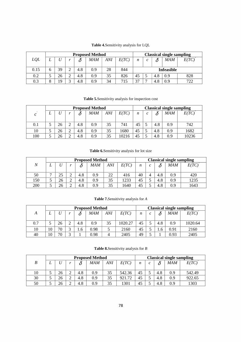
Table 4.Sensitivity analysis for LQL

Table 5.Sensitivity analysis for inspection cost

Table 6.Sensitivity analysis for lot size

Table 7.Sensitivity analysis for A

Table 8.Sensitivity analysis for B

LQL

Proposed Method Classical single sampling L U r δ MAM ANI E(TC) n c δ MAM E(TC)’

0.15 6 39 2 4.8 0.9 28 844 Infeasible 0.2 5 26 2 4.8 0.9 35 826 45 5 4.8 0.9 828 0.3 8 19 3 4.8 0.9 34 715 37 7 4.8 0.9 722

'c

Proposed Method Classical single sampling L U r δ MAM ANI E(TC) n c δ MAM E(TC)’

0.1 5 26 2 4.8 0.9 35 741 45 5 4.8 0.9 742

10 5 26 2 4.8 0.9 35 1680 45 5 4.8 0.9 1682 100 5 26 2 4.8 0.9 35 10216 45 5 4.8 0.9 10236

N

Proposed Method Classical single sampling L U r δ MAM ANI E(TC) n c δ MAM E(TC)’

50 7 25 2 4.8 0.9 22 416 40 4 4.8 0.9 420 150 5 26 2 4.8 0.9 35 1233 45 5 4.8 0.9 1235 200 5 26 2 4.8 0.9 35 1640 45 5 4.8 0.9 1643

A

Proposed Method Classical single sampling L U r δ MAM ANI E(TC) n c δ MAM E(TC)’

0.7 5 26 2 4.8 0.9 35 1020.27 45 5 4.8 0.9 1020.64

10 10 70 3 1.6 0.98 5 2160 45 5 1.6 0.91 2160 40 10 70 3 1 0.98 4 2405 49 5 1 0.93 2405

B

Proposed Method Classical single sampling L U r δ MAM ANI E(TC) n c δ MAM E(TC)’

10 5 26 2 4.8 0.9 35 542.36 45 5 4.8 0.9 542.49 30 5 26 2 4.8 0.9 35 921.72 45 5 4.8 0.9 922.65 50 5 26 2 4.8 0.9 35 1301 45 5 4.8 0.9 1303

79

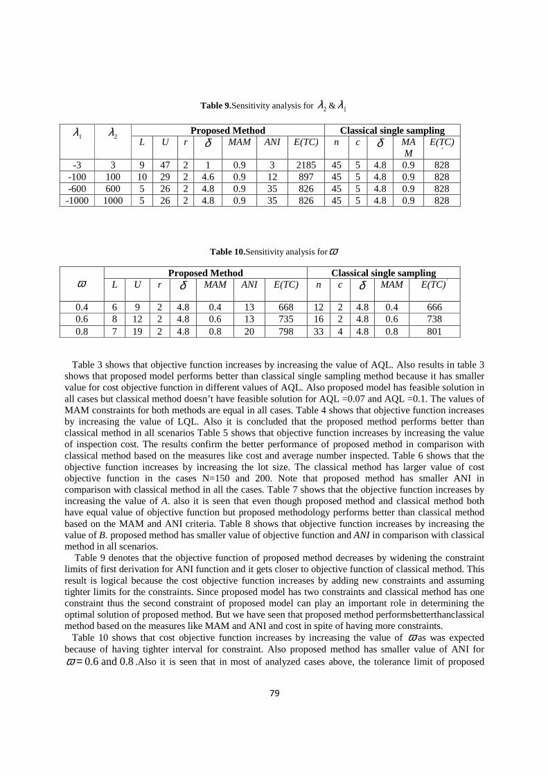
Table 9.Sensitivity analysis for 2λ & 1λ

Table 10.Sensitivity analysis forω

Table 3 shows that objective function increases by increasing the value of AQL. Also results in table 3 shows that proposed model performs better than classical single sampling method because it has smaller value for cost objective function in different values of AQL. Also proposed model has feasible solution in all cases but classical method doesn’t have feasible solution for AQL =0.07 and AQL =0.1. The values of MAM constraints for both methods are equal in all cases. Table 4 shows that objective function increases by increasing the value of LQL. Also it is concluded that the proposed method performs better than classical method in all scenarios Table 5 shows that objective function increases by increasing the value of inspection cost. The results confirm the better performance of proposed method in comparison with classical method based on the measures like cost and average number inspected. Table 6 shows that the objective function increases by increasing the lot size. The classical method has larger value of cost objective function in the cases N=150 and 200. Note that proposed method has smaller ANI in comparison with classical method in all the cases. Table 7 shows that the objective function increases by increasing the value of A. also it is seen that even though proposed method and classical method both have equal value of objective function but proposed methodology performs better than classical method based on the MAM and ANI criteria. Table 8 shows that objective function increases by increasing the value of B. proposed method has smaller value of objective function and ANI in comparison with classical method in all scenarios. Table 9 denotes that the objective function of proposed method decreases by widening the constraint limits of first derivation for ANI function and it gets closer to objective function of classical method. This result is logical because the cost objective function increases by adding new constraints and assuming tighter limits for the constraints. Since proposed model has two constraints and classical method has one constraint thus the second constraint of proposed model can play an important role in determining the optimal solution of proposed method. But we have seen that proposed method performsbetterthanclassical method based on the measures like MAM and ANI and cost in spite of having more constraints. Table 10 shows that cost objective function increases by increasing the value of ω as was expected because of having tighter interval for constraint. Also proposed method has smaller value of ANI for

0.6 and 0.8ω = .Also it is seen that in most of analyzed cases above, the tolerance limit of proposed

1λ 2λ Proposed Method Classical single sampling L U r δ MAM ANI E(TC) n c δ MA

M E(TC)

’ -3 3 9 47 2 1 0.9 3 2185 45 5 4.8 0.9 828

-100 100 10 29 2 4.6 0.9 12 897 45 5 4.8 0.9 828 -600 600 5 26 2 4.8 0.9 35 826 45 5 4.8 0.9 828 -1000 1000 5 26 2 4.8 0.9 35 826 45 5 4.8 0.9 828

ω

Proposed Method Classical single sampling L U r δ MAM ANI E(TC) n c δ MAM E(TC)’

0.4 6 9 2 4.8 0.4 13 668 12 2 4.8 0.4 666 0.6 8 12 2 4.8 0.6 13 735 16 2 4.8 0.6 738 0.8 7 19 2 4.8 0.8 20 798 33 4 4.8 0.8 801

80

method and classical method are the same that this result can confirm the validity of results. Another merit of proposed method is to generate feasible solutions for all analyzed cases.

5- Computational experiment In this section we are going to compare the results of proposed method with classical single sampling in 100 different scenarios of input parameters. 100 different scenarios of parameters are randomly generated by uniform distribution. The results are summarized in table “A” in appendix. According to Table “A”, ANI values of proposed method is less than their corresponding values in classical single sampling plan (n) for all of the cases. Also it is seen that classical method does not have any infeasible solution in 12% of cases while proposed method has feasible solution in all of the cases. Also proposed method has better objective function in 6% of cases but proposed model is worse than classical method in 4% of cases and for the rest of the cases, the objective function of these two methods are equal. Also the optimal values of δ in proposed method and classical method are equal in 96% of cases. As mentioned, minimum angle method (MAM) is an important characteristic of any sampling system thus it’s necessary to compare the results of two methods regarding this important criterion

( ( ) ( )a aP AQL P LQL− ). According to Table “A”, the proposed model has larger value of MAM measure

in 77% of cases and two methods have the same performance in the 4 % of cases thus the proposed method performs better than traditional method in approximately 80% of cases. This is another advantage and merit of proposed methodology. 6- Discussion Since the proposed model has three integer decision parameters thus optimization method for solving proposed sampling model is simple and just by a simple search method we can easily determine the optimal solution but the main focus of proposed model is to optimize different aspects of quality control simultaneously. First idea is to use conforming run length as a measure for decision making about quality of items. This idea has been successfully applied in many quality problems but applying this measure in an optimization model is not addressed before. Second contribution is to consider qualitative criteria and quantitative criteria of sampling model in an optimization model. The model considers all types of cost and risk functions which may occur in a sampling system. Even though there are some optimization models for sampling system in literature but most of them applied classical approach in a very limited model. Their approach includes specifying two points on OC curve or designing economically optimal sampling system. These models cannot determine the optimal solution for decision maker who consider risk and cost together along with inspection process and loss for both sides of contract. The main contribution of this research is to compare two different methods of acceptance sampling in quality control. We have shown that sampling based on CRL performed better than (n,c) classical sampling system. The comparison of these two sampling systems has been performed in several researches but we have shown that if all important aspects of an acceptance sampling problem were considered in an optimization model then sampling based on CRL would perform better than classical (n,c) design in most of the conditions. The resulted optimization model is not just obtained by considering some important key factors of sampling problems in a complex optimization model. The hidden and important idea is to propose a conceptual model for designing economically and statistically optimal acceptance sampling plan. As explained, CCC charts based on CRL has been widely used in process control but using this concept in acceptance sampling methods is not widely addressed and it is necessary to illustrate its advantages and disadvantages. Also, the criterion MAM is not widely applied in quality control problem while it is an important factor for designing statistically optimal sampling system. Other factors like risk and cost and loss have been considered in the model that helps the decision maker to select a proper decision by considering all important factors. All acceptance sampling models are simple optimization problems. The objective of these optimization problems is to minimize number of inspected items regarding LTPD or AOQ constraints. Acceptance sampling based on CRL can be a suitable alternative for classic l Dodge-Romig (n,c) sampling system (Fallahnezhad and Ahmadi Yazdi, 2015) .

81

The optimization model of classical (n,c) sampling systems is very limited with one objective function and one constraint. In this research a generalized economical optimization model based on CRL was developed for sampling system. The objective function and constraints are designed in order to consider most important characteristic of acceptance sampling problems. Fallahnezhad and Niaki (2013) have compared classical (n,c) design with CRL method based on cost objective function. They have shown that these two methods do not have identical performance and the CRL method performs better than classical method in some cases. Aslam et al.[26] have compared CRL method and classical sampling system based on ARL objective function. They have shown that CRL method performs better than classical sampling method in most of the cases. As for the best of author’s knowledge, there has not been a general comparison study between these two sampling systems so that we cannot compare the risk, the cost and the sample size of these two methods. Thus, we have developed a generalized optimization problem considering these key factors to analyse and compare the performance of these two methods in order to identify the merits of them based on some simulated case studies. The results of comparison study are summarized in table 11. Second column denotes the percentage of simulated cases studies where proposed method performs better than classical sampling systems and the results in third column denotes the percentage of cases which the classical sampling systems has the better performance. It is observed that the results are in favour of applying CRL sampling systems based on all important criteria of a sampling system.

Table 11. The results of comparing classical model and proposed method

Comparison Indexes

Proposed method

classical method Equal performance

Existing feasible solution

100% 87% -

E(TC) 6% 4% 90%

MAM 77% 19% 4%

ANI 100% 0% 0%

The proposed model can be applied as a new tool in quality control environment where classical models cannot provide guarantee for both producer and consumer, also adding other constraints or objective to the optimization model and solving this model is very simple.

7- Conclusion In this paper, a nonlinear optimization model is developed for obtaining the optimal threshold for tolerance design of products along with decision parameters of sampling method. The concept of cumulative run length of conforming items is employed for decision making in many cases. It is tried to optimize several objectives like the total loss, average number inspection, producer risk and consumer risk in one model where some objective are included in the constraints of the model by defining desired thresholds. It is observed that ANI values of proposed method are less than their corresponding values in classical single sampling plan for all of the simulated cases. Also it is seen that proposed method has better objective function in 6% of cases but proposed model is worse than classical method in 4% of cases and for the rest of the cases, the objective function of these two methods are equal. Also the optimal values of tolerance threshold in proposed method and classical method are equal in 96% of cases. Also it is seen that proposed model has larger value of MAM measure in 77% of cases and two methods have the same performance in the 4 % of cases thus we can sure that proposed method can perform better that

82

purposed method in approximately 80% of cases. Also it is seen that classical method does not have any infeasible solution in 12% of cases while proposed method has feasible solution in all of the cases. References

AhmadiYazdi A.,Fallahnezhad M.S. (2014),An optimization model for designing Acceptance Sampling Plan Based on Cumulative Count of Conforming Run Length Using Minimum Angle Method;Hacettepe Journal of Mathematics and Statistics 44(5); 1271-1281. AmirhosseinAmiri, RamezanKhosravi. (2012),Estimating the change point of the cumulative count of a conforming control chart under a drift;ScientiaIranica 19 (3); 856–861. Arizono I., Kanagawa A., Ohta H., WatakabeK., Tateishi K. (1997),Variable sampling plans for normal distribution indexed by Taguchi's loss function;Naval Research Logistics 44(6); 591-603. Aslam M, Fallahnezhad MS, Azam M. (2013),Decision Procedure for the Weibull Distribution based on Run Lengths of Conforming Items;Journal of Testing and Evaluation 41(5); 826-832. Bourke P.D. (2002),A continuous sampling plan using CUSUMs;Journal of Applied Statistics29(8); 1121-1133. Bourke P.D. (2003),A continuous sampling plan using sums of conforming run-lengths;Quality and Reliability Engineering International 19(1);53–66. Bowling, S.R.,Khasawneh, M.T.,Kaewkuekool, S.,Cho B.R. (2004),A Markovian approach to determining optimum process target levels for a multi-stage serial production system, European Journal of Operational Research 159(3); 636-650. Bush N., Leonard E. J., Marchan JR M. Q. M. (1953), A method of discrimination for single and double sampling OC curves utilizing the tangent at the point of inflection;Chemical Corps Engineering Agency, USA. Calvin TW. (1983),Quality control techniques for ‘zero-defects;IEEE Transactions on Components, Hybrids, and Manufacturing Technology 6;323–328.

Chen J.T. (2013),Design of cumulative count of conforming charts for high yield processes based on average number of items inspected;International Journal of Quality & Reliability Management 30(9);942 – 957. Elsayed E. A., Chen A. (1994),An economic design of control chart using quadratic loss function; International Journal of Production Research 32(4); 873-887.

Fallahnezhad MS, Niaki STA, Abooie MH. (2011),A New Acceptance Sampling Plan Based on Cumulative Sums of Conforming Run-Lengths;Journal of Industrial and Systems Engineering 4(4); 256-264. Fallahnezhad MS, HosseiniNasab H. (2011),Designing a Single Stage Acceptance Sampling Plan based on the control Threshold policy;International Journal of Industrial Engineering & Production Research 22(3); 143-150.

83

Fallahnezhad MS. (2012), A new Markov Chain Based Acceptance Sampling Policy via the Minimum Angle Method; Iranian Journal of Operations Research 3(1); 104-111. Fallahnezhad MS, HosseiniNasab H. (2012),A New Bayesian Acceptance Sampling Plan with Considering Inspection Errors;ScientiaIranica 19(6); 1865-1869. Fallahnezhad M.S.,Fakhrzad M.B. (2012),Determining an Economically Optimal (n,c) Design Via Using Loss Functions,International Journal of Engineering 25(3); 197-201. Fallahnezhad MS, Niaki STA, VahdatZad MA. (2012),A New Acceptance Sampling Design Using Bayesian Modeling and Backwards Induction, International Journal of Engineering 25(1); 45-54. Fallahnezhad M.S., AslamM. (2013),A New Economical Design of Acceptance Sampling Models Using Bayesian Inference;Accreditation and Quality Assurance 18(3); 187-195. Fallahnezhad M.S.,Niaki STA. (2013),A New Acceptance Sampling Policy Based on Number of Successive Conforming Items;Communications in Statistics-Theory and Methods 42(8); 1542-1552.

Fallahnezhad MS, Sajjadieh M, Abdollahi P. (2014),An iterative decision rule to minimize cost of acceptance sampling plan in machine replacement problem;International Journal of Engineering 27(7); 1099-1106. Fallahnezhad M.S. Ahmadi E. (2014),Optimal Process Adjustment with Considering Variable Costs for uni-variate and multi-variate Production Process;International Journal of Engineering 27(4); 561–572. Fallahnezhad MS, AhmadiYazdi A. (2015), Comparison between count of cumulative conforming sampling plans and Dodge-Romig single sampling plan; Communications in Statistics-Theory and Methods,In press. Fallahnezhad MS, A. AhmadiYazdi. (2015),Economic design of Acceptance Sampling Plans based on Conforming Run Lengths using Loss Functions;Journal of Testing and Evaluation 44(1); 1-8, Ferrell W.G., Chhoker Jr.A. (2002), Design of economically optimal acceptance sampling plans with inspection error; Computers & Operations Research 29(10); 1283-1300. Goh T. N. (1987),A control chart for very high yield processes;Quality Assurance 13; 18–22. Kobayashia J.,Arizonoa I., Takemotoa Y. (2003),Economical operation of control chart indexed by Taguchi's loss function;International Journal of Production Research 41(6); 1115-1132. Kuralmani V., Xie M., Goh T. N., Gan F. F. (2001),A conditional decision procedure for high yield processes;IIE Transactions 34; 1021–1030. Ling-Yau Chan, ShaominWub. (2009),Optimal design for inspection and maintenance policy based on the CCC chart;Computers & Industrial Engineering 57(3); 667–676.

84

Min Zhang, GuohuaNie, Zhen He. (2014),Performance of cumulative count of conforming chart of variable sampling intervalswith estimated control limits;International Journal of Production Economics 150;114–124. Mirabi M, Fallahnezhad MS. (2012),Analyzing Acceptance Sampling Plan by Markov Chains;South African Journal of Industrial Engineering 23(1);151-161. Moskowitz H., Tang K. (1992), Bayesian variables acceptance-sampling plans: quadratic loss function and step loss function; Technometrics 34(3); 340-347. Noorossana R., Saghaei A., Paynabar K., Samimi Y. (2007), On the conditional decision procedure for high yield processes;Computers and Industrial Engineering 53(3); 469–477. Sotiris Bersimis, Markos V. Koutras, Petros E. Maravelakis. (2013),A compound control chart for monitoring and controlling high quality processes;European Journal of Operational Research 233(3); 595–603. Soundararajan V, Christina AL. (1997), Selection of single sampling variables plans based on the minimum angle;Journal of Applied Statistics 24(2); 207-218. Taguchi G. Chowdhury S. Wu Y. (2005),Taguchi's Quality Engineering Handbook. Quality Loss Function; John Wiley & Sons 171 -198. Wu Z.,Shamsuzzamana M., Panb E.S. (2004),Optimization design of control charts based on Taguchi's loss function and random process shifts;International Journal of Production Research 42(2); 379-390. Xie M., Goh T. N. (1992), Some procedures for decision making in controlling high yield processes;Quality and Reliability Engineering International 8;355–360. Yan-Kwang Chen. (2013), Cumulative conformance count charts with variable sampling intervals for correlated samples;Computers & Industrial Engineering 64(1); 302–308. Zhang M., Peng Y.M., SchuhA., Megahed F.M., Woodall W.H. (2013),Geometric charts with estimated control limits;Quality and Reliability Engineering International 29 (2); 209–223. Zhang Wua, ZhaoJun Wang, Wei Jiang. (2010),A generalized Conforming Run Length control chart for monitoring the mean of a variable;Computers & Industrial Engineering 59(2); 185–192.

67

Appendix:

Table “A”. Proposed method VS. Classical single sampling

Scenarios

Input Parameters Proposed Method Classical single sampling

AQL LQL C1 N A B λ w L U r δ MAM ANI E(TC) n c δ MAM E(TC)’

1 0.02 0.21 7.7 63 44.2 28 6 0.87 10 70 3 1 0.99 4 2093 50 6 1 0.92 2093

2 0.04 0.15 88.1 81 22.5 19 539 0.9 8 48 2 1 0.9 3 8553 Infeasible 3 0.03 0.16 11.8 64 17.1 49 498 0.79 10 70 3 1.6 0.99 4 3274 48 5 1.6 0.79 3274 4 0.1 0.23 91.1 196 18.9 36 588 0.52 10 58 3 1.4 0.51 4 23876 50 10 1.4 0.58 23876 5 0.09 0.25 15.7 200 16.8 54 530 0.78 3 34 3 4.6 0.81 5 10489 50 6 1.8 0.83 11812 6 0.02 0.27 62.8 91 9.8 49 29 0.65 10 44 3 2.2 0.99 5 9032 45 2 2.2 0.93 9032 7 0.05 0.24 82.3 85 6.2 29 381 0.64 7 11 2 2.2 0.64 3 8836 11 1 2.2 0.66 8836 8 0.08 0.22 23.5 60 11.2 39 59 0.75 6 36 2 1.8 0.74 3 3251 50 7 1.8 0.84 3251 9 0.06 0.2 4 70 29 52 107 0.72 10 39 2 1.4 0.72 3 3343 45 6 1.4 0.81 3343 10 0.07 0.13 90.5 146 5.2 26 359 0.56 6 33 2 2.2 0.6 3 16068 Infeasible 11 0.02 0.24 77.9 91 25 20 406 0.87 10 70 3 1 0.99 4 8695 43 6 1 0.92 8695 12 0.05 0.14 31 129 33.1 56 546 0.78 8 70 3 1.2 0.95 4 10196 Infeasible 13 0.02 0.24 6.6 190 43.7 12 465 0.7 10 70 3 1 0.99 4 3656 50 9 1 0.77 3656 14 0.02 0.19 82.6 186 11.5 13 18 0.72 10 70 3 1 0.99 4 17584 37 4 1 0.84 17584 15 0.08 0.2 73.4 166 19.8 39 360 0.9 8 52 3 1.4 0.9 4 17640 Infeasible 16 0.05 0.26 12.2 150 9.5 36 505 0.64 3 34 3 4.6 0.88 5 3241 50 4 2 0.9 6083 17 0.06 0.2 8.2 102 29.7 13 553 0.57 10 70 3 1 0.9 4 2134 50 8 1 0.67 2134 18 0.04 0.21 3 104 3 29 7 0.9 9 47 2 2.6 0.9 4 2683 50 4 3.2 0.93 2639 19 0.01 0.21 11.6 121 14.4 60 402 0.76 5 70 1 2 0.86 2 6993 46 3 2 0.98 6993 20 0.08 0.23 41.9 196 44.4 60 391 0.89 8 49 3 1.2 0.9 4 18464 Infeasible 21 0.1 0.24 26.7 121 14 33 73 0.67 3 70 3 1.6 0.96 10 6544 49 7 1.6 0.84 6531 22 0.03 0.25 0.7 111 14.4 56 87 0.59 10 70 3 2 0.99 5 4932 50 4 22 0.98 4932 23 0.04 0.19 75.9 127 45.7 49 193 0.89 9 70 3 1 0.98 4 15148 50 5 1 0.9 15148 24 0.03 0.24 62.3 119 2.2 38 577 0.73 10 18 3 4.8 0.74 25 7528 29 5 4.8 0.73 7593 25 0.07 0.23 4.4 99 7.7 31 146 0.72 7 70 3 2 0.89 5 2800 50 5 2 0.82 2800 26 0.02 0.16 11.4 125 15.7 57 39 0.57 10 70 3 2 0.99 5 7091 49 4 2 0.91 7091 27 0.02 0.26 31 132 4.5 23 193 0.91 10 70 3 2.2 0.99 5 6328 47 3 2.2 0.99 6328 28 0.03 0.28 78.3 136 15.9 44 518 0.59 10 70 3 1.6 0.99 4 15521 49 8 1.6 0.95 15521 29 0.08 0.2 83.2 193 23.9 41 209 0.51 10 70 3 1.4 0.67 4 22801 50 9 1.4 0.54 22801 30 0.09 0.19 82.6 67 19 52 488 0.87 3 70 3 1.6 0.97 10 8321 Infeasible

85

68

31 0.04 0.14 28.5 81 9.1 34 221 0.77 10 70 3 2 0.97 5 4480 50 4 2 0.79 4480 32 0.05 0.23 48.8 93 40.4 17 155 0.77 6 70 3 1 0.99 4 6018 50 8 1 0.85 6018 33 0.04 0.17 94.3 76 35.1 36 145 0.73 10 70 3 1 0.98 4 9590 50 6 1 0.77 9590 34 0.05 0.26 48.1 197 25.1 32 576 0.52 10 70 3 1.2 0.97 4 14929 49 10 1.2 0.75 14929 35 0.08 0.17 36 62 31.5 55 225 0.65 10 70 3 1.4 0.66 4 5112 49 5 1.4 0.65 5112 36 0.04 0.23 13.8 192 15 13 74 0.87 9 70 3 1 0.98 4 4916 49 7 1 0.91 4916 37 0.08 0.2 38.7 85 37.7 49 183 0.51 8 70 3 1.2 0.7 4 6956 47 8 1.2 0.6 6956 38 0.09 0.15 91.9 65 31.2 46 516 0.52 10 60 3 1.2 0.53 4 8506 Infeasible 39 0.03 0.14 90 135 46.8 13 143 0.68 10 70 3 1 0.97 4 13943 50 5 1 0.69 13943 40 0.07 0.27 48.3 155 41.1 55 210 0.84 7 70 3 1.2 0.94 4 14871 47 9 1.2 0.85 14871 41 0.1 0.17 87.9 62 21.7 28 384 0.52 9 63 3 1.2 0.57 4 6907 50 7 1.2 0.54 6907 42 0.06 0.24 58.9 192 4.3 52 227 0.8 8 23 3 4.8 0.79 45 15878 42 7 4.8 0.8 15953 43 0.04 0.25 26.2 169 19.6 10 214 0.79 8 70 3 1 0.99 4 6056 47 8 1 0.85 6056 44 0.06 0.28 83.7 196 5.5 30 174 0.53 6 15 3 4.8 0.55 30 16531 32 8 4.8 0.54 16384 45 0.04 0.24 82.6 138 14 47 34 0.81 7 70 3 1.8 0.99 5 16507 50 7 1.8 0.94 16507 46 0.1 0.23 72.3 187 30.5 30 33 0.53 10 58 3 1 0.53 4 18579 49 10 1 0.59 18579 47 0.07 0.3 90.3 200 9.7 21 424 0.63 10 70 3 1.4 0.74 4 21565 43 7 1.4 0.95 21565 48 0.04 0.29 87.4 102 41.8 56 400 0.89 10 70 3 1.2 0.99 4 13947 47 9 1.2 0.92 13947 49 0.07 0.22 57 133 42.1 53 540 0.84 10 70 3 1.2 0.85 4 13778 41 5 1.2 0.86 13778 50 0.03 0.14 72.4 124 8.5 56 422 0.63 3 15 1 2.6 0.64 2 13897 19 1 2.6 0.63 13897 51 0.06 0.15 83.3 130 4.8 47 435 0.72 6 29 2 3.2 0.72 5 14756 49 4 3.2 0.72 14756 52 0.02 0.16 40.3 166 18.2 24 35 0.86 5 70 2 1.2 0.98 3 10221 50 4 1.2 0.9 10221 53 0.05 0.16 66.9 150 38.3 27 202 0.55 10 70 3 1 0.96 4 13763 45 6 1 0.56 13763 54 0.05 0.18 43.9 123 18.2 22 469 0.52 10 70 3 1 0.94 4 7744 50 8 1 0.52 7744 55 0.09 0.16 42.8 184 12.2 30 482 0.58 10 65 3 1.6 0.57 4 12369 Infeasible 56 0.08 0.24 4.5 130 39.7 56 308 0.76 8 70 3 1.2 0.82 4 6844 50 9 1.2 0.77 6844 57 0.04 0.28 51.3 92 26.3 24 592 0.73 10 70 3 1 0.97 4 6681 50 10 1 0.85 6681 58 0.04 0.15 46 174 38.8 18 282 0.5 7 70 3 1 0.98 4 10961 41 5 1 0.61 10961 59 0.01 0.12 15.2 186 18.1 55 398 0.77 9 70 3 1.8 0.94 4 11044 50 3 1.8 0.87 11044 60 0.03 0.21 20 172 5.7 11 347 0.58 3 70 2 1.4 0.99 3 5075 32 2 1.4 0.88 5075 61 0.06 0.26 2.7 85 16.2 39 369 0.68 9 70 3 1.6 0.92 4 3017 50 7 1.6 0.95 3017 62 0.04 0.22 11.5 72 46.8 45 520 0.82 6 70 3 1 0.99 4 3676 46 7 1 0.82 3676 63 0.08 0.21 20.1 135 45.9 36 241 0.9 7 60 3 1 0.9 4 7121 Infeasible 64 0.06 0.21 22.9 107 10.3 35 163 0.69 10 70 3 1.8 0.93 4 5491 50 6 1.8 0.9 5491 65 0.07 0.21 76.9 137 49.4 59 440 0.63 9 70 3 1 0.79 4 17682 50 8 1 0.73 17682 66 0.02 0.17 30.5 178 12.7 21 125 0.72 10 70 3 1.2 0.99 4 8693 50 6 1.2 0.75 8693 67 0.07 0.13 62.1 130 24.8 18 288 0.61 6 70 3 1 0.85 4 10184 Infeasible 68 0.01 0.16 23.8 72 25.3 59 144 0.59 3 70 3 1.6 0.91 10 5253 50 6 1.6 0.73 5253

86

69

69 0.09 0.29 19.9 109 16 28 471 0.69 10 49 3 1.4 0.7 4 4749 50 9 1.4 0.92 4749 70 0.03 0.27 84.6 163 32.7 26 290 0.89 9 70 3 1 0.99 4 17680 50 9 1 0.9 17680 71 0.03 0.26 91.3 178 45.2 41 265 0.87 9 70 3 1 0.99 4 22742 50 8 1 0.93 22742 72 0.02 0.28 38.2 73 6.8 53 442 0.57 6 52 2 2.8 0.99 4 5484 50 1 2.8 0.79 5484 73 0.06 0.17 37.6 128 34.2 14 512 0.76 4 70 3 1 0.98 4 6519 50 5 1 0.8 6519 74 0.04 0.18 46.7 187 14.3 21 256 0.83 9 70 3 1.2 0.98 4 12193 48 5 1.2 0.87 12193 75 0.03 0.29 66.4 189 18 51 388 0.52 3 70 3 1.6 0.99 10 20466 49 7 1.6 0.98 20466 76 0.05 0.24 9.9 167 6.9 16 332 0.75 3 70 3 1.6 0.99 10 3911 40 4 1.6 0.9 3911 77 0.01 0.25 90.3 128 23.8 45 287 0.74 10 70 3 1.4 0.99 4 16461 50 10 1.4 0.75 16461 78 0.05 0.26 11.8 199 46.4 43 120 0.68 10 70 3 1 0.97 4 9961 45 9 1 0.78 9961 79 0.06 0.29 23.5 89 9.6 53 471 0.92 10 70 3 2.4 0.93 5 5552 50 5 2.4 0.93 5552 80 0.06 0.16 16.2 149 42.6 20 352 0.59 10 70 3 1 0.91 4 5203 50 6 1 0.65 5203 81 0.07 0.22 37.6 141 4.6 38 343 0.57 9 11 2 3 0.56 4 8931 15 2 3 0.59 8934 82 0.03 0.27 75.4 136 28.9 24 445 0.87 10 70 3 1 0.99 4 13174 44 8 1 0.88 13174 83 0.09 0.22 3.8 198 20.2 28 283 0.68 8 70 3 1.2 0.69 4 5520 50 9 1.2 0.68 5520 84 0.06 0.16 98.1 73 47.3 50 112 0.54 7 63 2 1 0.55 3 10451 50 6 1 0.63 10451 85 0.02 0.14 11.7 170 1.7 56 7 0.53 6 8 1 3.6 0.54 3 6499 14 1 4.8 0.56 5307 86 0.03 0.3 25 162 38.4 23 103 0.77 9 70 3 1 0.99 4 7504 50 10 1 0.91 7504 87 0.04 0.13 43.4 170 32.5 29 411 0.8 10 70 3 1 0.95 4 11796 Infeasible 88 0.07 0.25 4.4 173 4.4 37 565 0.58 10 70 3 3 0.77 6 5096 50 4 3 0.69 5096 89 0.04 0.21 48.5 76 47.4 13 524 0.57 6 70 3 1 0.99 4 4730 43 8 1 0.56 4730 90 0.03 0.15 58.7 139 7.1 19 68 0.86 9 70 2 1.6 0.95 3 10300 50 4 1.6 0.87 10300 91 0.08 0.25 77.5 72 40 26 217 0.88 10 45 3 1 0.88 4 7293 50 8 1 0.89 7293 92 0.09 0.28 88.7 165 41.9 32 52 0.54 10 60 3 1 0.54 4 19441 50 10 1 0.85 19441 93 0.04 0.28 54.9 108 2.1 12 564 0.72 4 12 2 4.8 0.72 22 5191 25 5 4.8 0.72 5224 94 0.04 0.13 99 145 42 59 256 0.52 4 70 2 1.2 0.95 3 21811 36 3 1.2 0.64 21811 95 0.02 0.16 63.6 116 38.4 41 526 0.67 10 70 3 1 0.99 4 11585 29 3 1 0.72 11585 96 0.01 0.17 56.1 100 43.4 42 58 0.76 9 70 3 1 0.99 4 9307 50 6 1 0.78 9307 97 0.07 0.16 37.3 100 33.6 25 233 0.64 10 70 3 1 0.8 4 5970 50 6 1 0.65 5970 98 0.08 0.24 15.2 55 9.2 15 110 0.9 9 49 3 1.2 0.9 4 1536 Infeasible 99 0.04 0.26 75.1 66 36.8 20 451 0.8 7 70 3 1 0.99 4 6213 50 10 1 0.8 6213 100 0.01 0.14 91.2 187 41.1 34 461 0.63 9 70 3 1 0.98 4 22777 50 5 1 0.74 22777

87