A new neural network technique for the design of multilayered microwave shielded bandpass filters

A New Neural Network Technique for the Design ofMultilayered Microwave Shielded Bandpass Filters

Juan Pascual Garcıa, Fernando Quesada Pereira, David Canete Rebenaque,Juan Sebastian Gomez Dıaz, Alejandro Alvarez Melcon

Department of Information Technologies and Communications (TIC),Technical University of Cartagena, Cartagena, Murcia, Antiguo Cuartel de Antiguones 30202, Spain

Received 16 May 2008; accepted 27 October 2008

ABSTRACT: In this work, we propose a novel technique based on neural networks, for the

design of microwave filters in shielded printed technology. The technique uses radial basis

function neural networks to represent the non linear relations between the quality factors

and coupling coefficients, with the geometrical dimensions of the resonators. The radial basis

function neural networks are employed for the first time in the design task of shielded

printed filters, and permit a fast and precise operation with only a limited set of training

data. Thanks to a new cascade configuration, a set of two neural networks provide the

dimensions of the complete filter in a fast and accurate way. To improve the calculation of

the geometrical dimensions, the neural networks can take as inputs both electrical parame-

ters and physical dimensions computed by other neural networks. The neural network tech-

nique is combined with gradient based optimization methods to further improve the

response of the filters. Results are presented to demonstrate the usefulness of the proposed

technique for the design of practical microwave printed coupled line and hairpin

filters. VVC 2008 Wiley Periodicals, Inc. Int J RF and Microwave CAE 19: 405–415, 2009.

Keywords: neural networks; filter design; multilayered shielded structures; microwave filters

I. INTRODUCTION

Neural networks constitute one useful technique in

microwave filter modeling and design. The first appli-

cations of neural networks were focused on modeling

different microwave devices. In the design task, neu-

ral networks can be employed following two different

strategies. The first approach consists on using the

neural networks employed in the modeling task in an

inverse way [1]. In the second method, neural inputs

and outputs are interchanged with respect to the mod-

eling methodology. Thus, the inputs correspond to the

electrical response, and the outputs are the physical

dimensions. Therefore, this strategy is known as

direct inverse modeling. Some works have proved the

capability of neural networks to design microwave

devices such as, i.e., horn antennas [2] and filters [3].

In Refs. 4, 5, neural networks are used to approximate

the relations between some elements of a filter cou-

pling matrix and the physical dimensions that synthe-

size the mentioned coupling elements. The technique

was applied to design several waveguide pseudo-

elliptic filters. Neural networks have also been applied

to printed multilayer filter design. In Ref. 6, the tradi-

tional multilayer perceptron neural network is utilized

to obtain the geometrical dimensions of coupled line

filters, using as inputs some normal mode parameters

(such as impedance and voltage ratios).

Two of the most popular transfer functions used in

the design of practical filters are the Butterworth and

the Chebyshev responses. The lowpass prototype

Correspondence to: J. P. Garcıa; e-mail: [email protected] 10.1002/mmce.20363Published online 23 December 2008 in Wiley InterScience

(www.interscience.wiley.com).

VVC 2008 Wiley Periodicals, Inc.

405

filter elements corresponding to a given desired

response permit to evaluate the external quality fac-

tors and the coupling coefficients between all the res-

onators of the filter [7]. The main difficulty in the

final design of the filter lies on finding the resonators

dimensions, which synthesize the computed quality

factor and coupling coefficients. In the case of micro-

strip filters printed on substrates, with infinite trans-

verse dimensions, there exist empirical formulas that

allow to calculate the resonator dimensions using

look-up tables. For example, in the case of parallel

coupled lines, the dimensions are computed from the

even and odd impedance values [8]. In other cases,

the physical dimensions of the filter are obtained

from design curves that relate these dimensions with

the quality factors, coupling coefficients, and other

electrical parameters [8–10].

In shielded multilayered microstrip filters, the

transverse dimensions are finite, and there are no em-

pirical equations to compute easily the physical dimen-

sions of the filter. If the empirical equations corre-

sponding to the unshielded structure are employed, the

required precision is not usually attained. This is

because the shielding effects and the interactions with

the lateral walls are neglected. The construction of

new design curves for shielded printed filters requires

the calculation of a high number of quality factors and

coupling coefficient values, to reach enough precision

in the filter design task. These calculations can be per-

formed using full-wave analysis techniques, such as

the integral equation or the finite elements method.

However, such full-wave analysis techniques usually

consume high computational resources.

In this work, we propose the use of radial basis

function neural networks to learn the relations (in a

given frequency bandwidth) between the quality fac-

tor, resonant frequency, and coupling coefficients,

with their corresponding physical dimensions. In this

way, a limited number of quality factors and coupling

coefficients are needed to generate the information

required for the design of practical filters. Using the

novel technique, an initial amount of time is needed

to generate the neural networks training and testing

data. Furthermore, to largely reduce the training time,

the neural network method developed in Ref. 11 is

used during the calculation of the training data. Once

trained, different printed multilayer filters with center

frequency inside the operating bandwidth can be eas-

ily designed. The output of the neural network will

be, directly, the dimensions of the filter which synthe-

size a given transfer function. It is important to

remark that the training set generation and neural

training times are not included in the filter design

step. When a new filter is designed using the neural

networks, it is necessary neither to generate a new

training set nor to train the neural networks.

If the designed filter does not fulfill totally the spec-

ifications, then a fast optimization step is performed

based on gradient techniques. These methods have

been widely applied to the design of microwave cir-

cuits, i.e., in microstrip structures as in Refs. 12, 13.

Generally, the last step in a design process is the opti-

mization of an initial geometry [14]. The neural

method described in this article provides an initial ge-

ometry very close to the optimum. This will drastically

reduce the time invested in the optimization, assuring

at the same time a proper convergence of gradient base

algorithms (which strongly relies on a very good initial

point). The present method is not limited to a specific

type of printed filter as in Ref. 6. As results will show,

different hairpin and coupled line filters can be

designed employing the same methodology.

II. THEORY

Different steps are needed for the design of micro-

wave filters. First, the order of the filter is computed

from the specifications and from the desired transfer

function characteristics (typical transfer functions

include Butterworth, Chebyshev or Elliptic func-

tions). Second, the quality factors and coupling

coefficients are calculated with the element values of

the synthesized lowpass prototype filter. Finally, the

dimensions of the resonators are calculated to synthe-

size the required external quality factors and coupling

coefficients [7].

This last step is the most important and compli-

cated to carry out. Depending on the type of resonator

chosen to implement the filter, different structures

can be employed to calculate the quality factors and

coupling coefficients. Doubly and singly terminated

resonator structures can be used for the evaluation of

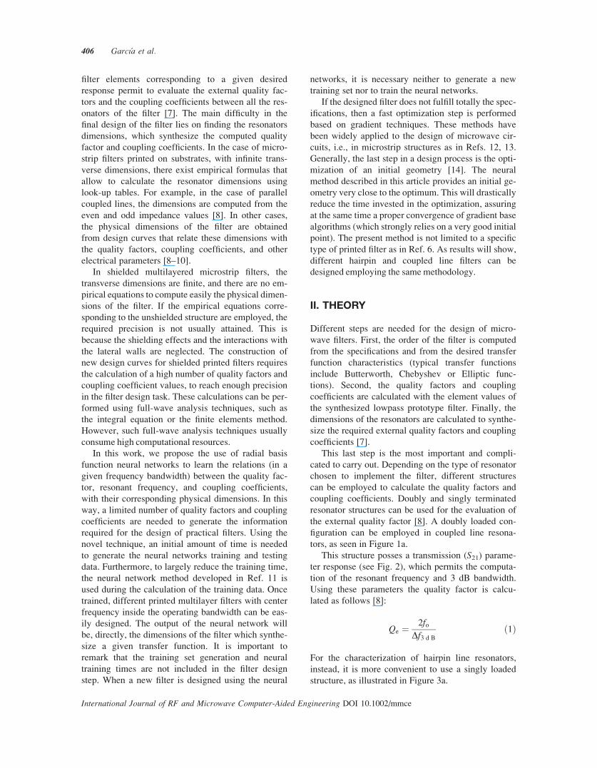
the external quality factor [8]. A doubly loaded con-

figuration can be employed in coupled line resona-

tors, as seen in Figure 1a.

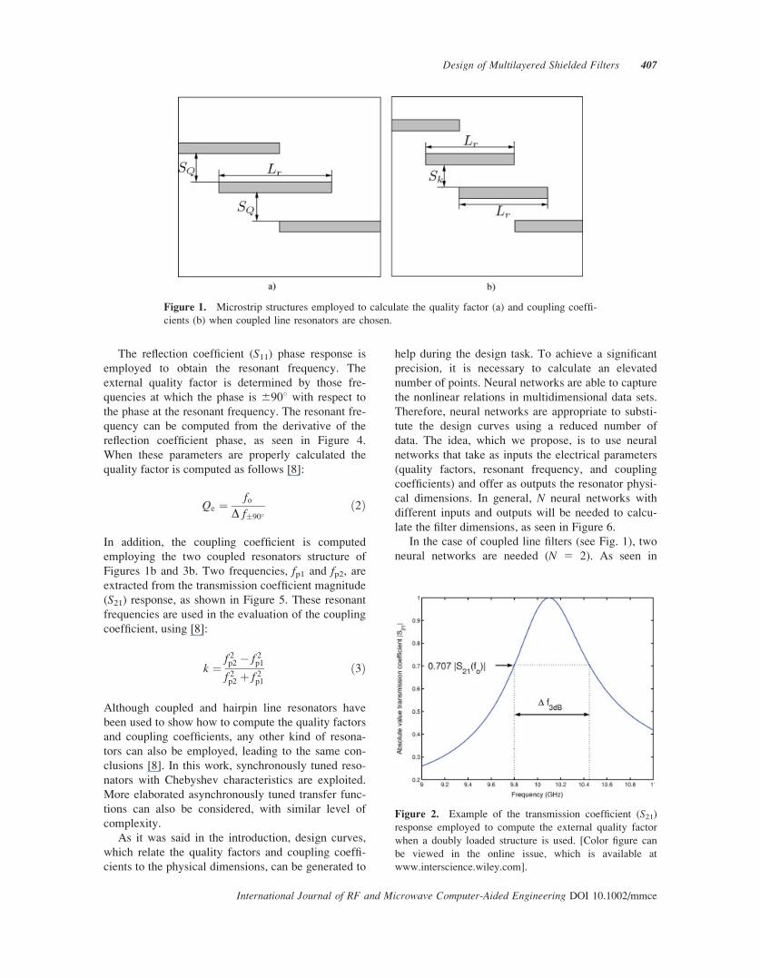
This structure posses a transmission (S21) parame-

ter response (see Fig. 2), which permits the computa-

tion of the resonant frequency and 3 dB bandwidth.

Using these parameters the quality factor is calcu-

lated as follows [8]:

Qe ¼2fo

Df3 d B

ð1Þ

For the characterization of hairpin line resonators,

instead, it is more convenient to use a singly loaded

structure, as illustrated in Figure 3a.

406 Garcıa et al.

International Journal of RF and Microwave Computer-Aided Engineering DOI 10.1002/mmce

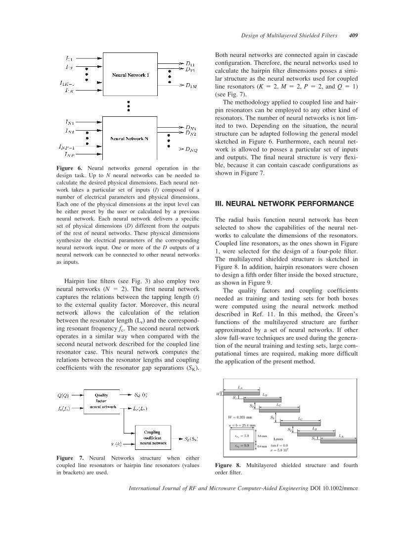
The reflection coefficient (S11) phase response is

employed to obtain the resonant frequency. The

external quality factor is determined by those fre-

quencies at which the phase is 6908 with respect to

the phase at the resonant frequency. The resonant fre-

quency can be computed from the derivative of the

reflection coefficient phase, as seen in Figure 4.

When these parameters are properly calculated the

quality factor is computed as follows [8]:

Qe ¼fo

D f�90�ð2Þ

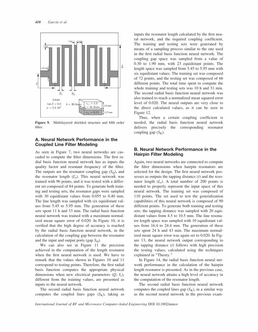
In addition, the coupling coefficient is computed

employing the two coupled resonators structure of

Figures 1b and 3b. Two frequencies, fp1 and fp2, are

extracted from the transmission coefficient magnitude

(S21) response, as shown in Figure 5. These resonant

frequencies are used in the evaluation of the coupling

coefficient, using [8]:

k ¼f 2p2 � f 2

p1

f 2p2 þ f 2

p1

ð3Þ

Although coupled and hairpin line resonators have

been used to show how to compute the quality factors

and coupling coefficients, any other kind of resona-

tors can also be employed, leading to the same con-

clusions [8]. In this work, synchronously tuned reso-

nators with Chebyshev characteristics are exploited.

More elaborated asynchronously tuned transfer func-

tions can also be considered, with similar level of

complexity.

As it was said in the introduction, design curves,

which relate the quality factors and coupling coeffi-

cients to the physical dimensions, can be generated to

help during the design task. To achieve a significant

precision, it is necessary to calculate an elevated

number of points. Neural networks are able to capture

the nonlinear relations in multidimensional data sets.

Therefore, neural networks are appropriate to substi-

tute the design curves using a reduced number of

data. The idea, which we propose, is to use neural

networks that take as inputs the electrical parameters

(quality factors, resonant frequency, and coupling

coefficients) and offer as outputs the resonator physi-

cal dimensions. In general, N neural networks with

different inputs and outputs will be needed to calcu-

late the filter dimensions, as seen in Figure 6.

In the case of coupled line filters (see Fig. 1), two

neural networks are needed (N 5 2). As seen in

Figure 2. Example of the transmission coefficient (S21)

response employed to compute the external quality factor

when a doubly loaded structure is used. [Color figure can

be viewed in the online issue, which is available at

www.interscience.wiley.com].

Figure 1. Microstrip structures employed to calculate the quality factor (a) and coupling coeffi-

cients (b) when coupled line resonators are chosen.

Design of Multilayered Shielded Filters 407

International Journal of RF and Microwave Computer-Aided Engineering DOI 10.1002/mmce

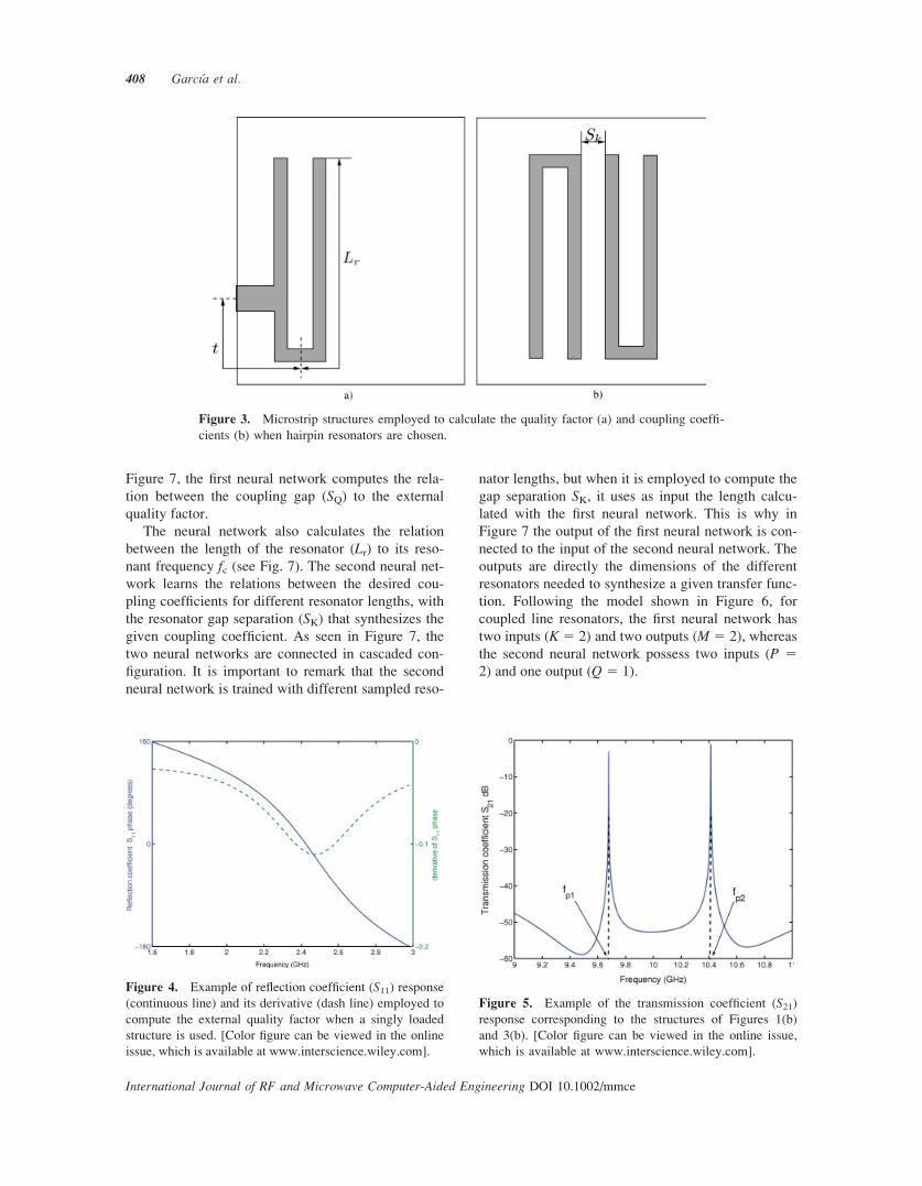
Figure 7, the first neural network computes the rela-

tion between the coupling gap (SQ) to the external

quality factor.

The neural network also calculates the relation

between the length of the resonator (Lr) to its reso-

nant frequency fc (see Fig. 7). The second neural net-

work learns the relations between the desired cou-

pling coefficients for different resonator lengths, with

the resonator gap separation (SK) that synthesizes the

given coupling coefficient. As seen in Figure 7, the

two neural networks are connected in cascaded con-

figuration. It is important to remark that the second

neural network is trained with different sampled reso-

nator lengths, but when it is employed to compute the

gap separation SK, it uses as input the length calcu-

lated with the first neural network. This is why in

Figure 7 the output of the first neural network is con-

nected to the input of the second neural network. The

outputs are directly the dimensions of the different

resonators needed to synthesize a given transfer func-

tion. Following the model shown in Figure 6, for

coupled line resonators, the first neural network has

two inputs (K 5 2) and two outputs (M 5 2), whereas

the second neural network possess two inputs (P 5

2) and one output (Q 5 1).

Figure 3. Microstrip structures employed to calculate the quality factor (a) and coupling coeffi-

cients (b) when hairpin resonators are chosen.

Figure 4. Example of reflection coefficient (S11) response

(continuous line) and its derivative (dash line) employed to

compute the external quality factor when a singly loaded

structure is used. [Color figure can be viewed in the online

issue, which is available at www.interscience.wiley.com].

Figure 5. Example of the transmission coefficient (S21)

response corresponding to the structures of Figures 1(b)

and 3(b). [Color figure can be viewed in the online issue,

which is available at www.interscience.wiley.com].

408 Garcıa et al.

International Journal of RF and Microwave Computer-Aided Engineering DOI 10.1002/mmce

Hairpin line filters (see Fig. 3) also employ two

neural networks (N 5 2). The first neural network

captures the relations between the tapping length (t)to the external quality factor. Moreover, this neural

network allows the calculation of the relation

between the resonator length (Lr) and the correspond-

ing resonant frequency fc. The second neural network

operates in a similar way when compared with the

second neural network described for the coupled line

resonator case. This neural network computes the

relations between the resonator lengths and coupling

coefficients with the resonator gap separations (SK).

Both neural networks are connected again in cascade

configuration. Therefore, the neural networks used to

calculate the hairpin filter dimensions posses a simi-

lar structure as the neural networks used for coupled

line resonators (K 5 2, M 5 2, P 5 2, and Q 5 1)

(see Fig. 7).

The methodology applied to coupled line and hair-

pin resonators can be employed to any other kind of

resonators. The number of neural networks is not lim-

ited to two. Depending on the situation, the neural

structure can be adapted following the general model

sketched in Figure 6. Furthermore, each neural net-

work is allowed to posses a particular set of inputs

and outputs. The final neural structure is very flexi-

ble, because it can contain cascade configurations as

shown in Figure 7.

III. NEURAL NETWORK PERFORMANCE

The radial basis function neural network has been

selected to show the capabilities of the neural net-

works to calculate the dimensions of the resonators.

Coupled line resonators, as the ones shown in Figure

1, were selected for the design of a four-pole filter.

The multilayered shielded structure is sketched in

Figure 8. In addition, hairpin resonators were chosen

to design a fifth order filter inside the boxed structure,

as shown in Figure 9.

The quality factors and coupling coefficients

needed as training and testing sets for both boxes

were computed using the neural network method

described in Ref. 11. In this method, the Green’s

functions of the multilayered structure are further

approximated by a set of neural networks. If other

slow full-wave techniques are used during the genera-

tion of the neural training and testing sets, large com-

putational times are required, making more difficult

the application of the present method.

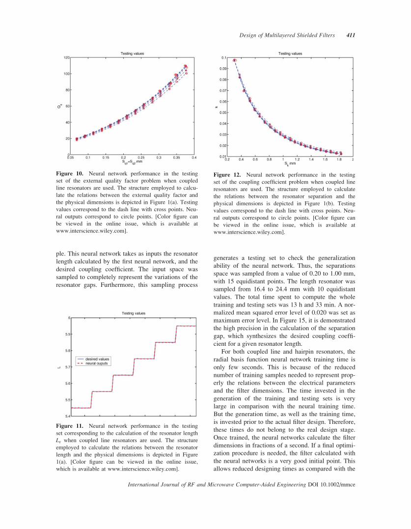
Figure 6. Neural networks general operation in the

design task. Up to N neural networks can be needed to

calculate the desired physical dimensions. Each neural net-

work takes a particular set of inputs (I) composed of a

number of electrical parameters and physical dimensions.

Each one of the physical dimensions at the input level can

be either preset by the user or calculated by a previous

neural network. Each neural network delivers a specific

set of physical dimensions (D) different from the outputs

of the rest of neural networks. These physical dimensions

synthesize the electrical parameters of the corresponding

neural network input. One or more of the D outputs of a

neural network can be connected to other neural networks

as inputs.

Figure 7. Neural Networks structure when either

coupled line resonators or hairpin line resonators (values

in brackets) are used.

Figure 8. Multilayered shielded structure and fourth

order filter.

Design of Multilayered Shielded Filters 409

International Journal of RF and Microwave Computer-Aided Engineering DOI 10.1002/mmce

A. Neural Network Performance in theCoupled Line Filter Modeling

As seen in Figure 7, two neural networks are cas-

caded to compute the filter dimensions. The first ra-

dial basis function neural network has as inputs the

quality factor and resonant frequency of the filter.

The outputs are the resonator coupling gap (SQ), and

the resonator length (Lr). This neural network was

trained with 96 points, and it was tested with a differ-

ent set composed of 84 points. To generate both train-

ing and testing sets, the resonator gaps were sampled

with 30 equidistant values from 0.055 to 0.40 mm.

The line length was sampled with six equidistant val-

ues from 5.45 to 5.95 mm. The generation of these

sets spent 11 h and 33 min. The radial basis function

neural network was trained with a maximum normal-

ized mean square error of 0.020. In Figure 10, it is

verified that the high degree of accuracy is reached

by the radial basis function neural network, in the

calculation of the coupling gap between the resonator

and the input and output ports (gap SQ).

We can also see in Figure 11 the precision

achieved in the computation of the length resonator

when the first neural network is used. We have to

remark that the values shown in Figures 10 and 11

correspond to testing points. Therefore, the first radial

basis function computes the appropriate physical

dimensions when new electrical parameters (Q, fc),

different from the training values, are presented as

inputs to the neural network.

The second radial basis function neural network

computes the coupled lines gaps (SK), taking as

inputs the resonator length calculated by the first neu-

ral network, and the required coupling coefficient.

The training and testing sets were generated by

means of a sampling process similar to the one used

in the first radial basis function neural network. The

coupling gap space was sampled from a value of

0.30 to 1.90 mm, with 23 equidistant points. The

length space was sampled from 5.45 to 5.95 mm with

six equidistant values. The training set was composed

of 72 points, and the testing set was composed of 66

different points. The total time spent to compute the

whole training and testing sets was 10 h and 31 min.

The second radial basis function neural network was

also trained to reach a normalized mean squared error

level of 0.020. The neural outputs are very close to

the direct calculated values, as it can be seen in

Figure 12.

Thus, when a certain coupling coefficient is

needed, the radial basis function neural network

delivers precisely the corresponding resonator

coupling gap (SK).

B. Neural Network Performance in theHairpin Filter Modeling

Again, two neural networks are connected to compute

the filter dimensions when hairpin resonators are

selected for the design. The first neural network pos-

sesses as outputs the tapping distance (t) and the reso-

nator length (Lr). A total number of 200 points is

needed to properly represent the input space of this

neural network. The training set was composed of

110 points. The set used to test the generalization

capabilities of this neural network is composed of 90

different points. To generate both training and testing

sets, the tapping distance was sampled with 20 equi-

distant values from 4.5 to 10.5 mm. The line resona-

tor length space was sampled with 10 equidistant val-

ues from 16.4 to 24.4 mm. The generation of these

sets spent 24 h and 43 min. The maximum normal-

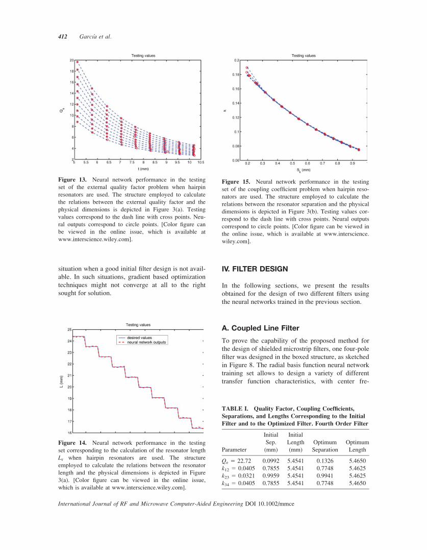
ized mean square error was again set to 0.020. In Fig-

ure 13, the neural network output corresponding to

the tapping distance (t) follows with high precision

the testing values, calculated using the techniques

explained in ‘‘Theory.’’

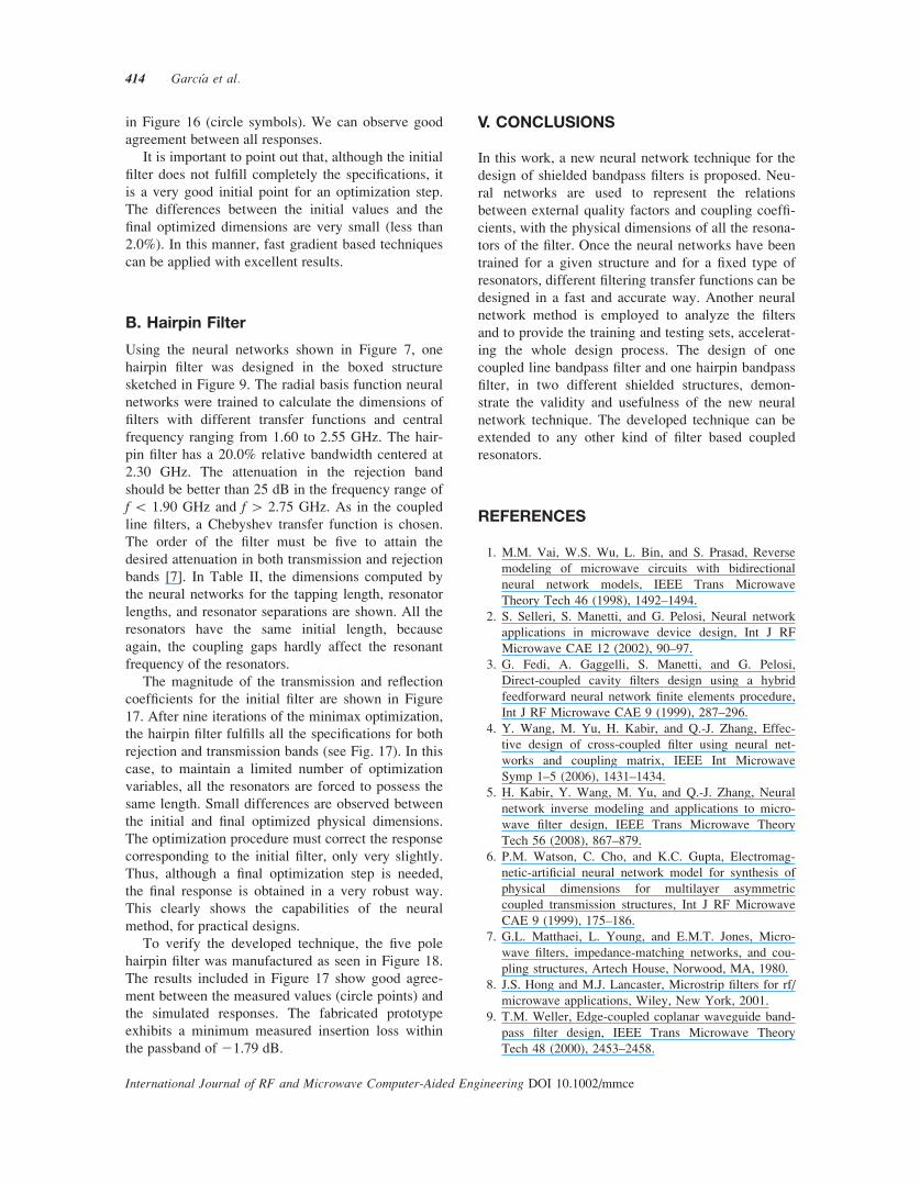
In Figure 14, the radial basis function neural net-

work performance in the calculation of the hairpin

length resonator is presented. As in the previous case,

the neural network attains a high level of accuracy in

the computation of the resonator length.

The second radial basis function neural network

computes the coupled lines gap (SK), in a similar way

as the second neural network in the previous exam-

Figure 9. Multilayered shielded structure and fifth order

filter.

410 Garcıa et al.

International Journal of RF and Microwave Computer-Aided Engineering DOI 10.1002/mmce

ple. This neural network takes as inputs the resonator

length calculated by the first neural network, and the

desired coupling coefficient. The input space was

sampled to completely represent the variations of the

resonator gaps. Furthermore, this sampling process

generates a testing set to check the generalization

ability of the neural network. Thus, the separations

space was sampled from a value of 0.20 to 1.00 mm,

with 15 equidistant points. The length resonator was

sampled from 16.4 to 24.4 mm with 10 equidistant

values. The total time spent to compute the whole

training and testing sets was 13 h and 33 min. A nor-

malized mean squared error level of 0.020 was set as

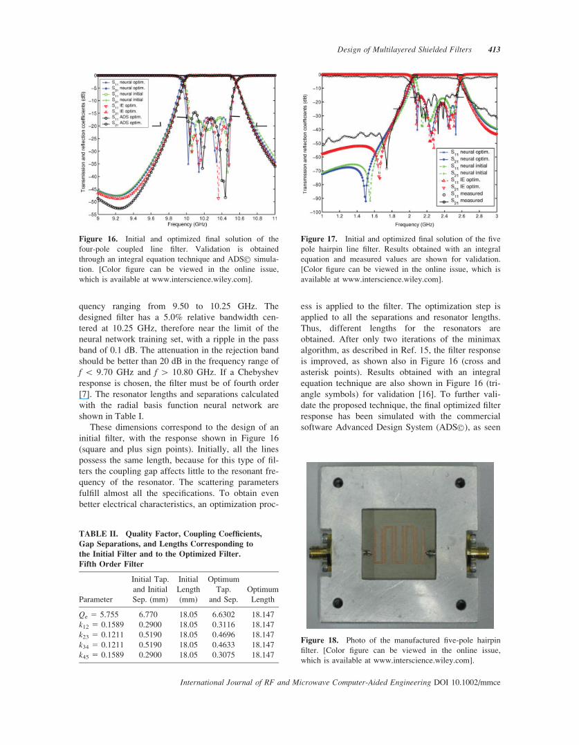
maximum error level. In Figure 15, it is demonstrated

the high precision in the calculation of the separation

gap, which synthesizes the desired coupling coeffi-

cient for a given resonator length.

For both coupled line and hairpin resonators, the

radial basis function neural network training time is

only few seconds. This is because of the reduced

number of training samples needed to represent prop-

erly the relations between the electrical parameters

and the filter dimensions. The time invested in the

generation of the training and testing sets is very

large in comparison with the neural training time.

But the generation time, as well as the training time,

is invested prior to the actual filter design. Therefore,

these times do not belong to the real design stage.

Once trained, the neural networks calculate the filter

dimensions in fractions of a second. If a final optimi-

zation procedure is needed, the filter calculated with

the neural networks is a very good initial point. This

allows reduced designing times as compared with the

Figure 12. Neural network performance in the testing

set of the coupling coefficient problem when coupled line

resonators are used. The structure employed to calculate

the relations between the resonator separation and the

physical dimensions is depicted in Figure 1(b). Testing

values correspond to the dash line with cross points. Neu-

ral outputs correspond to circle points. [Color figure can

be viewed in the online issue, which is available at

www.interscience.wiley.com].

Figure 10. Neural network performance in the testing

set of the external quality factor problem when coupled

line resonators are used. The structure employed to calcu-

late the relations between the external quality factor and

the physical dimensions is depicted in Figure 1(a). Testing

values correspond to the dash line with cross points. Neu-

ral outputs correspond to circle points. [Color figure can

be viewed in the online issue, which is available at

www.interscience.wiley.com].

Figure 11. Neural network performance in the testing

set corresponding to the calculation of the resonator length

Lr when coupled line resonators are used. The structure

employed to calculate the relations between the resonator

length and the physical dimensions is depicted in Figure

1(a). [Color figure can be viewed in the online issue,

which is available at www.interscience.wiley.com].

Design of Multilayered Shielded Filters 411

International Journal of RF and Microwave Computer-Aided Engineering DOI 10.1002/mmce

situation when a good initial filter design is not avail-

able. In such situations, gradient based optimization

techniques might not converge at all to the right

sought for solution.

IV. FILTER DESIGN

In the following sections, we present the results

obtained for the design of two different filters using

the neural networks trained in the previous section.

A. Coupled Line Filter

To prove the capability of the proposed method for

the design of shielded microstrip filters, one four-pole

filter was designed in the boxed structure, as sketched

in Figure 8. The radial basis function neural network

training set allows to design a variety of different

transfer function characteristics, with center fre-

Figure 14. Neural network performance in the testing

set corresponding to the calculation of the resonator length

Lr when hairpin resonators are used. The structure

employed to calculate the relations between the resonator

length and the physical dimensions is depicted in Figure

3(a). [Color figure can be viewed in the online issue,

which is available at www.interscience.wiley.com].

Figure 15. Neural network performance in the testing

set of the coupling coefficient problem when hairpin reso-

nators are used. The structure employed to calculate the

relations between the resonator separation and the physical

dimensions is depicted in Figure 3(b). Testing values cor-

respond to the dash line with cross points. Neural outputs

correspond to circle points. [Color figure can be viewed in

the online issue, which is available at www.interscience.

wiley.com].

Figure 13. Neural network performance in the testing

set of the external quality factor problem when hairpin

resonators are used. The structure employed to calculate

the relations between the external quality factor and the

physical dimensions is depicted in Figure 3(a). Testing

values correspond to the dash line with cross points. Neu-

ral outputs correspond to circle points. [Color figure can

be viewed in the online issue, which is available at

www.interscience.wiley.com].

TABLE I. Quality Factor, Coupling Coefficients,

Separations, and Lengths Corresponding to the Initial

Filter and to the Optimized Filter. Fourth Order Filter

Parameter

Initial

Sep.

(mm)

Initial

Length

(mm)

Optimum

Separation

Optimum

Length

Qe 5 22.72 0.0992 5.4541 0.1326 5.4650

k12 5 0.0405 0.7855 5.4541 0.7748 5.4625

k23 5 0.0321 0.9959 5.4541 0.9941 5.4625

k34 5 0.0405 0.7855 5.4541 0.7748 5.4650

412 Garcıa et al.

International Journal of RF and Microwave Computer-Aided Engineering DOI 10.1002/mmce

quency ranging from 9.50 to 10.25 GHz. The

designed filter has a 5.0% relative bandwidth cen-

tered at 10.25 GHz, therefore near the limit of the

neural network training set, with a ripple in the pass

band of 0.1 dB. The attenuation in the rejection band

should be better than 20 dB in the frequency range of

f \ 9.70 GHz and f [ 10.80 GHz. If a Chebyshev

response is chosen, the filter must be of fourth order

[7]. The resonator lengths and separations calculated

with the radial basis function neural network are

shown in Table I.

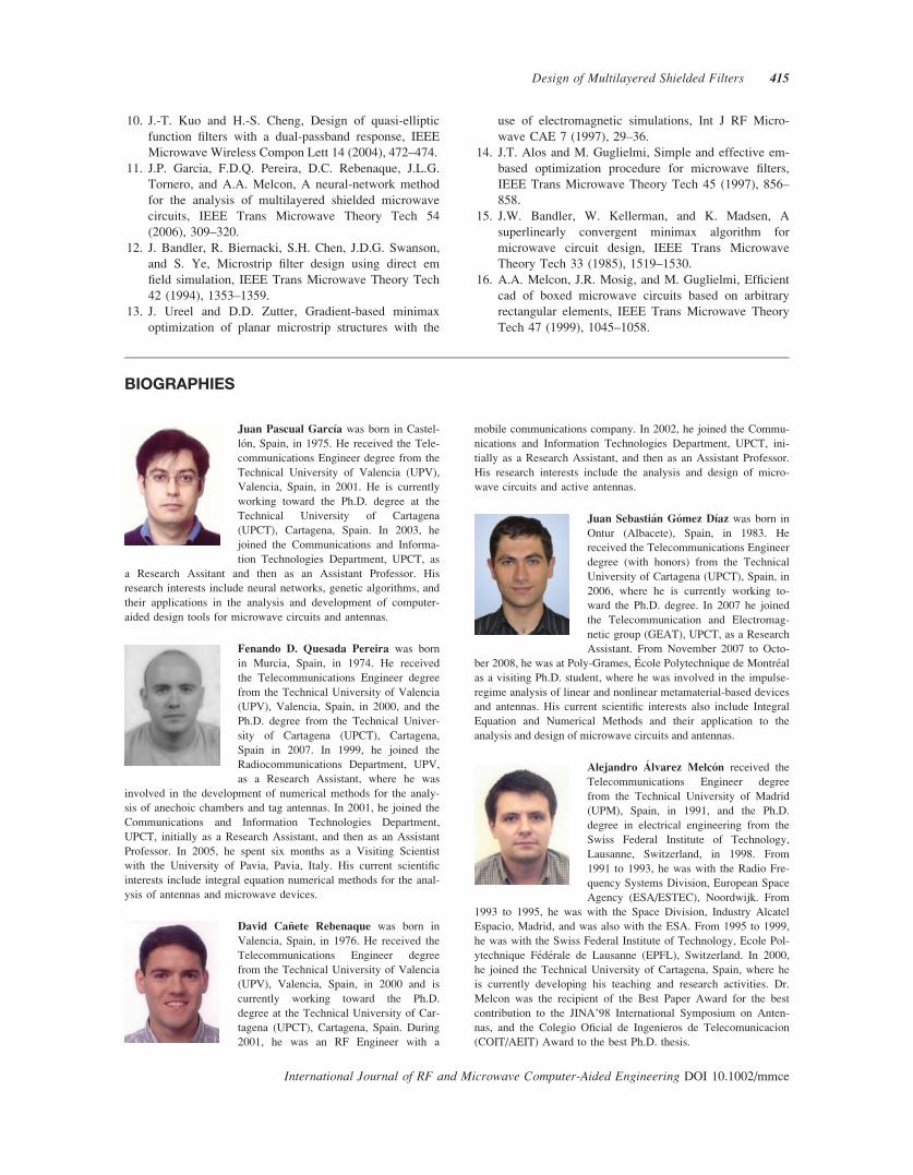
These dimensions correspond to the design of an

initial filter, with the response shown in Figure 16

(square and plus sign points). Initially, all the lines

possess the same length, because for this type of fil-

ters the coupling gap affects little to the resonant fre-

quency of the resonator. The scattering parameters

fulfill almost all the specifications. To obtain even

better electrical characteristics, an optimization proc-

ess is applied to the filter. The optimization step is

applied to all the separations and resonator lengths.

Thus, different lengths for the resonators are

obtained. After only two iterations of the minimax

algorithm, as described in Ref. 15, the filter response

is improved, as shown also in Figure 16 (cross and

asterisk points). Results obtained with an integral

equation technique are also shown in Figure 16 (tri-

angle symbols) for validation [16]. To further vali-

date the proposed technique, the final optimized filter

response has been simulated with the commercial

software Advanced Design System (ADS�), as seen

Figure 16. Initial and optimized final solution of the

four-pole coupled line filter. Validation is obtained

through an integral equation technique and ADS� simula-

tion. [Color figure can be viewed in the online issue,

which is available at www.interscience.wiley.com].

TABLE II. Quality Factor, Coupling Coefficients,

Gap Separations, and Lengths Corresponding to

the Initial Filter and to the Optimized Filter.

Fifth Order Filter

Parameter

Initial Tap.

and Initial

Sep. (mm)

Initial

Length

(mm)

Optimum

Tap.

and Sep.

Optimum

Length

Qe 5 5.755 6.770 18.05 6.6302 18.147

k12 5 0.1589 0.2900 18.05 0.3116 18.147

k23 5 0.1211 0.5190 18.05 0.4696 18.147

k34 5 0.1211 0.5190 18.05 0.4633 18.147

k45 5 0.1589 0.2900 18.05 0.3075 18.147

Figure 17. Initial and optimized final solution of the five

pole hairpin line filter. Results obtained with an integral

equation and measured values are shown for validation.

[Color figure can be viewed in the online issue, which is

available at www.interscience.wiley.com].

Figure 18. Photo of the manufactured five-pole hairpin

filter. [Color figure can be viewed in the online issue,

which is available at www.interscience.wiley.com].

Design of Multilayered Shielded Filters 413

International Journal of RF and Microwave Computer-Aided Engineering DOI 10.1002/mmce

in Figure 16 (circle symbols). We can observe good

agreement between all responses.

It is important to point out that, although the initial

filter does not fulfill completely the specifications, it

is a very good initial point for an optimization step.

The differences between the initial values and the

final optimized dimensions are very small (less than

2.0%). In this manner, fast gradient based techniques

can be applied with excellent results.

B. Hairpin Filter

Using the neural networks shown in Figure 7, one

hairpin filter was designed in the boxed structure

sketched in Figure 9. The radial basis function neural

networks were trained to calculate the dimensions of

filters with different transfer functions and central

frequency ranging from 1.60 to 2.55 GHz. The hair-

pin filter has a 20.0% relative bandwidth centered at

2.30 GHz. The attenuation in the rejection band

should be better than 25 dB in the frequency range of

f \ 1.90 GHz and f [ 2.75 GHz. As in the coupled

line filters, a Chebyshev transfer function is chosen.

The order of the filter must be five to attain the

desired attenuation in both transmission and rejection

bands [7]. In Table II, the dimensions computed by

the neural networks for the tapping length, resonator

lengths, and resonator separations are shown. All the

resonators have the same initial length, because

again, the coupling gaps hardly affect the resonant

frequency of the resonators.

The magnitude of the transmission and reflection

coefficients for the initial filter are shown in Figure

17. After nine iterations of the minimax optimization,

the hairpin filter fulfills all the specifications for both

rejection and transmission bands (see Fig. 17). In this

case, to maintain a limited number of optimization

variables, all the resonators are forced to possess the

same length. Small differences are observed between

the initial and final optimized physical dimensions.

The optimization procedure must correct the response

corresponding to the initial filter, only very slightly.

Thus, although a final optimization step is needed,

the final response is obtained in a very robust way.

This clearly shows the capabilities of the neural

method, for practical designs.

To verify the developed technique, the five pole

hairpin filter was manufactured as seen in Figure 18.

The results included in Figure 17 show good agree-

ment between the measured values (circle points) and

the simulated responses. The fabricated prototype

exhibits a minimum measured insertion loss within

the passband of 21.79 dB.

V. CONCLUSIONS

In this work, a new neural network technique for the

design of shielded bandpass filters is proposed. Neu-

ral networks are used to represent the relations

between external quality factors and coupling coeffi-

cients, with the physical dimensions of all the resona-

tors of the filter. Once the neural networks have been

trained for a given structure and for a fixed type of

resonators, different filtering transfer functions can be

designed in a fast and accurate way. Another neural

network method is employed to analyze the filters

and to provide the training and testing sets, accelerat-

ing the whole design process. The design of one

coupled line bandpass filter and one hairpin bandpass

filter, in two different shielded structures, demon-

strate the validity and usefulness of the new neural

network technique. The developed technique can be

extended to any other kind of filter based coupled

resonators.

REFERENCES

1. M.M. Vai, W.S. Wu, L. Bin, and S. Prasad, Reverse

modeling of microwave circuits with bidirectional

neural network models, IEEE Trans Microwave

Theory Tech 46 (1998), 1492–1494.

2. S. Selleri, S. Manetti, and G. Pelosi, Neural network

applications in microwave device design, Int J RF

Microwave CAE 12 (2002), 90–97.

3. G. Fedi, A. Gaggelli, S. Manetti, and G. Pelosi,

Direct-coupled cavity filters design using a hybrid

feedforward neural network finite elements procedure,

Int J RF Microwave CAE 9 (1999), 287–296.

4. Y. Wang, M. Yu, H. Kabir, and Q.-J. Zhang, Effec-

tive design of cross-coupled filter using neural net-

works and coupling matrix, IEEE Int Microwave

Symp 1–5 (2006), 1431–1434.

5. H. Kabir, Y. Wang, M. Yu, and Q.-J. Zhang, Neural

network inverse modeling and applications to micro-

wave filter design, IEEE Trans Microwave Theory

Tech 56 (2008), 867–879.

6. P.M. Watson, C. Cho, and K.C. Gupta, Electromag-

netic-artificial neural network model for synthesis of

physical dimensions for multilayer asymmetric

coupled transmission structures, Int J RF Microwave

CAE 9 (1999), 175–186.

7. G.L. Matthaei, L. Young, and E.M.T. Jones, Micro-

wave filters, impedance-matching networks, and cou-

pling structures, Artech House, Norwood, MA, 1980.

8. J.S. Hong and M.J. Lancaster, Microstrip filters for rf/

microwave applications, Wiley, New York, 2001.

9. T.M. Weller, Edge-coupled coplanar waveguide band-

pass filter design, IEEE Trans Microwave Theory

Tech 48 (2000), 2453–2458.

414 Garcıa et al.

International Journal of RF and Microwave Computer-Aided Engineering DOI 10.1002/mmce

10. J.-T. Kuo and H.-S. Cheng, Design of quasi-elliptic

function filters with a dual-passband response, IEEE

Microwave Wireless Compon Lett 14 (2004), 472–474.

11. J.P. Garcia, F.D.Q. Pereira, D.C. Rebenaque, J.L.G.

Tornero, and A.A. Melcon, A neural-network method

for the analysis of multilayered shielded microwave

circuits, IEEE Trans Microwave Theory Tech 54

(2006), 309–320.

12. J. Bandler, R. Biernacki, S.H. Chen, J.D.G. Swanson,

and S. Ye, Microstrip filter design using direct em

field simulation, IEEE Trans Microwave Theory Tech

42 (1994), 1353–1359.

13. J. Ureel and D.D. Zutter, Gradient-based minimax

optimization of planar microstrip structures with the

use of electromagnetic simulations, Int J RF Micro-

wave CAE 7 (1997), 29–36.

14. J.T. Alos and M. Guglielmi, Simple and effective em-

based optimization procedure for microwave filters,

IEEE Trans Microwave Theory Tech 45 (1997), 856–

858.

15. J.W. Bandler, W. Kellerman, and K. Madsen, A

superlinearly convergent minimax algorithm for

microwave circuit design, IEEE Trans Microwave

Theory Tech 33 (1985), 1519–1530.

16. A.A. Melcon, J.R. Mosig, and M. Guglielmi, Efficient

cad of boxed microwave circuits based on arbitrary

rectangular elements, IEEE Trans Microwave Theory

Tech 47 (1999), 1045–1058.

BIOGRAPHIES

Juan Pascual Garcıa was born in Castel-

lon, Spain, in 1975. He received the Tele-

communications Engineer degree from the

Technical University of Valencia (UPV),

Valencia, Spain, in 2001. He is currently

working toward the Ph.D. degree at the

Technical University of Cartagena

(UPCT), Cartagena, Spain. In 2003, he

joined the Communications and Informa-

tion Technologies Department, UPCT, as

a Research Assitant and then as an Assistant Professor. His

research interests include neural networks, genetic algorithms, and

their applications in the analysis and development of computer-

aided design tools for microwave circuits and antennas.

Fenando D. Quesada Pereira was born

in Murcia, Spain, in 1974. He received

the Telecommunications Engineer degree

from the Technical University of Valencia

(UPV), Valencia, Spain, in 2000, and the

Ph.D. degree from the Technical Univer-

sity of Cartagena (UPCT), Cartagena,

Spain in 2007. In 1999, he joined the

Radiocommunications Department, UPV,

as a Research Assistant, where he was

involved in the development of numerical methods for the analy-

sis of anechoic chambers and tag antennas. In 2001, he joined the

Communications and Information Technologies Department,

UPCT, initially as a Research Assistant, and then as an Assistant

Professor. In 2005, he spent six months as a Visiting Scientist

with the University of Pavia, Pavia, Italy. His current scientific

interests include integral equation numerical methods for the anal-

ysis of antennas and microwave devices.

David Canete Rebenaque was born in

Valencia, Spain, in 1976. He received the

Telecommunications Engineer degree

from the Technical University of Valencia

(UPV), Valencia, Spain, in 2000 and is

currently working toward the Ph.D.

degree at the Technical University of Car-

tagena (UPCT), Cartagena, Spain. During

2001, he was an RF Engineer with a

mobile communications company. In 2002, he joined the Commu-

nications and Information Technologies Department, UPCT, ini-

tially as a Research Assistant, and then as an Assistant Professor.

His research interests include the analysis and design of micro-

wave circuits and active antennas.

Juan Sebastian Gomez Dıaz was born in

Ontur (Albacete), Spain, in 1983. He

received the Telecommunications Engineer

degree (with honors) from the Technical

University of Cartagena (UPCT), Spain, in

2006, where he is currently working to-

ward the Ph.D. degree. In 2007 he joined

the Telecommunication and Electromag-

netic group (GEAT), UPCT, as a Research

Assistant. From November 2007 to Octo-

ber 2008, he was at Poly-Grames, Ecole Polytechnique de Montreal

as a visiting Ph.D. student, where he was involved in the impulse-

regime analysis of linear and nonlinear metamaterial-based devices

and antennas. His current scientific interests also include Integral

Equation and Numerical Methods and their application to the

analysis and design of microwave circuits and antennas.

Alejandro Alvarez Melcon received the

Telecommunications Engineer degree

from the Technical University of Madrid

(UPM), Spain, in 1991, and the Ph.D.

degree in electrical engineering from the

Swiss Federal Institute of Technology,

Lausanne, Switzerland, in 1998. From

1991 to 1993, he was with the Radio Fre-

quency Systems Division, European Space

Agency (ESA/ESTEC), Noordwijk. From

1993 to 1995, he was with the Space Division, Industry Alcatel

Espacio, Madrid, and was also with the ESA. From 1995 to 1999,

he was with the Swiss Federal Institute of Technology, Ecole Pol-

ytechnique Federale de Lausanne (EPFL), Switzerland. In 2000,

he joined the Technical University of Cartagena, Spain, where he

is currently developing his teaching and research activities. Dr.

Melcon was the recipient of the Best Paper Award for the best

contribution to the JINA’98 International Symposium on Anten-

nas, and the Colegio Oficial de Ingenieros de Telecomunicacion

(COIT/AEIT) Award to the best Ph.D. thesis.

Design of Multilayered Shielded Filters 415

International Journal of RF and Microwave Computer-Aided Engineering DOI 10.1002/mmce