A new moving average approach to predict the direction of ...

Journal of New Results in Science 11(1) (2022) 13-25

A new moving average approach to predict the direction of stock

movements in algorithmic trading

Üzeyir Aycel1 , Yunus Santur2

Keywords:

Algorithmic trading,

Financial forecasting,

Stock market,

Technical analysis

Abstract − Moving averages and indicators derived from these averages are used to predict the

future direction the stocks will move. In manual and algorithmic trading, moving averages play

a decisive role in decision making. In this study, a new hybrid approach has been developed

that can be used as an alternative to moving averages such as SMA, WMA and EMA used in the

literature. In BIST30 stocks in Turkey, the proposed method performs better than widely used

indicators such as MACD, Stochastic and RSI, commonly used in the literature.

Subject Classification (2020): 62P05, 91G15.

1. Introduction

Trading transactions in financial markets are carried out autonomously through robots called manual

or algorithmic systems [1]. Real investors decide according to basic expectations, trend analysis,

formations, and indicators in manual transactions. Past experiences could affect these decisions either

positively or negatively [2]. Autonomous systems, devoid of emotions and making much faster

decisions, open trades using these indicator data. Autonomous systems can open high-frequency

transactions for much shorter periods. Investors use these systems to avoid negative factors such as

following screens, making fast and correct decisions in variable conditions, and under stress in sudden

price changes. In recent years, a significant part of the market transaction volumes has been generated

by these autonomous systems [3].

Nowadays, the number of systems using computational intelligence, such as deep learning, is

increasing day by day [4]. These systems, which are much more complex, aim to identify trend

patterns formed by time series and predict price movements based on artificial intelligence by

developing models that learn from indicator data [5]. The disadvantage of these systems is that they

have to work in real-time, and the hardware costs of the models are relatively high. On the other hand,

indicators derived from moving averages consist of simple but effective mathematical models using

statistical methods. In this way, they are easier to calculate in real-time, and since buy/sell strategies

are rule-based, they can be programmed more easily. Moreover, it is easier and faster to perform tasks

[email protected] (Corresponding Author); [email protected] 1,2Department of Software Engineering, Faculty of Technology, Fırat University, Elazığ, Turkey Article History: Received: 06 Aug 2021 — Accepted: 02 Feb 2022 — Published: 30 Apr 2022

Journal of New Results in Science

https://dergipark.org.tr/en/pub/jnrs

Research Article

Open Access

E-ISSN:1304-7981 https://doi.org/10.54187/jnrs.979836

VOLUME 11:

NUMBER 1:

YEAR 2022:

http://dergipark.gov.tr/jnrs

[email protected]

14

Aycel and Santur / JNRS / 11(1) (2022) 13-25

such as Backtest used to test the strategy created and optimise for selecting the best parameters to

maximise portfolio earnings [6].

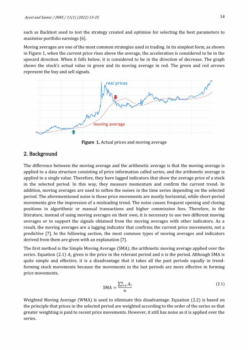
Moving averages are one of the most common strategies used in trading. In its simplest form, as shown

in Figure 1, when the current price rises above the average, the acceleration is considered to be in the

upward direction. When it falls below, it is considered to be in the direction of decrease. The graph

shows the stock’s actual value in green and its moving average in red. The green and red arrows

represent the buy and sell signals.

Figure 1. Actual prices and moving average

2. Background

The difference between the moving average and the arithmetic average is that the moving average is

applied to a data structure consisting of price information called series, and the arithmetic average is

applied to a single value. Therefore, they have lagged indicators that show the average price of a stock

in the selected period. In this way, they measure momentum and confirm the current trend. In

addition, moving averages are used to soften the noises in the time series depending on the selected

period. The aforementioned noise is those price movements are mostly horizontal, while short-period

movements give the impression of a misleading trend. The noise causes frequent opening and closing

positions in algorithmic or manual transactions and higher commission fees. Therefore, in the

literature, instead of using moving averages on their own, it is necessary to use two different moving

averages or to support the signals obtained from the moving averages with other indicators. As a

result, the moving averages are a lagging indicator that confirms the current price movements, not a

predictive [7]. In the following section, the most common types of moving averages and indicators

derived from them are given with an explanation [7].

The first method is the Simple Moving Average (SMA), the arithmetic moving average applied over the

series. Equation (2.1) 𝐴𝑖 given is the price in the relevant period and n is the period. Although SMA is

quite simple and effective, it is a disadvantage that it takes all the past periods equally in trend-

forming stock movements because the movements in the last periods are more effective in forming

price movements.

SMA =∑ 𝐴𝑖

𝑛𝑖=1

𝑛

(2.1)

Weighted Moving Average (WMA) is used to eliminate this disadvantage. Equation (2.2) is based on

the principle that prices in the selected period are weighted according to the order of the series so that

greater weighting is paid to recent price movements. However, it still has noise as it is applied over the

series.

15

Aycel and Santur / JNRS / 11(1) (2022) 13-25

WMA =∑ 𝐴𝑖(𝑛 − 𝑖)1

𝑖=𝑛

𝑛(𝑛 + 1) 2⁄ (2.2)

Exponential Moving Average (EMA) reduces the noise and expresses the latest price movements more

heavily. Since the EMA is calculated recursively based on the previous period, it provides a good

smoothing in which the noise decreases more. Since the recursion is calculated as Equation (2.3), the

previous day’s EMA value is needed, so SMA is used instead of the first EMA value.

EMA𝑡 = 𝐴𝑡 (2

𝑛 + 1) + EMA𝑡−1 (1 −

2

𝑛 + 1)

(2.3)

The three different MA formula commonly used in the literature is given above. In fact, EMA is a

special form of WMA, and the principle of all moving averages is how to choose their weights.

However, double or triple EMA is commonly used for more softening, as in Equation (2.4) and

Equation (2.5).

DEMA = 2EMA − EMA(EMA) (2.4)

TEMA = 3EMA − 3EMA(EMA) + EMA(EMA(EMA)) (2.5)

As a general acceptance, it is more appropriate to choose WMA and EMA for periods of 20 or less and

SMA for periods of 60 or longer since the final prices are more important. Because as the period grows,

the weights selected according to the WMA and EMA principle converge to the SMA. The shorter the

selected period, the higher the possibility of noise and false signals will cause a delay. This delay will

typically result in an uptrend entering the position late (after prices have risen) and late exit (after

prices have fallen). This situation is shown in Figure 1; when the actual prices fall below the moving

average, the profitable position is exited with some loss.

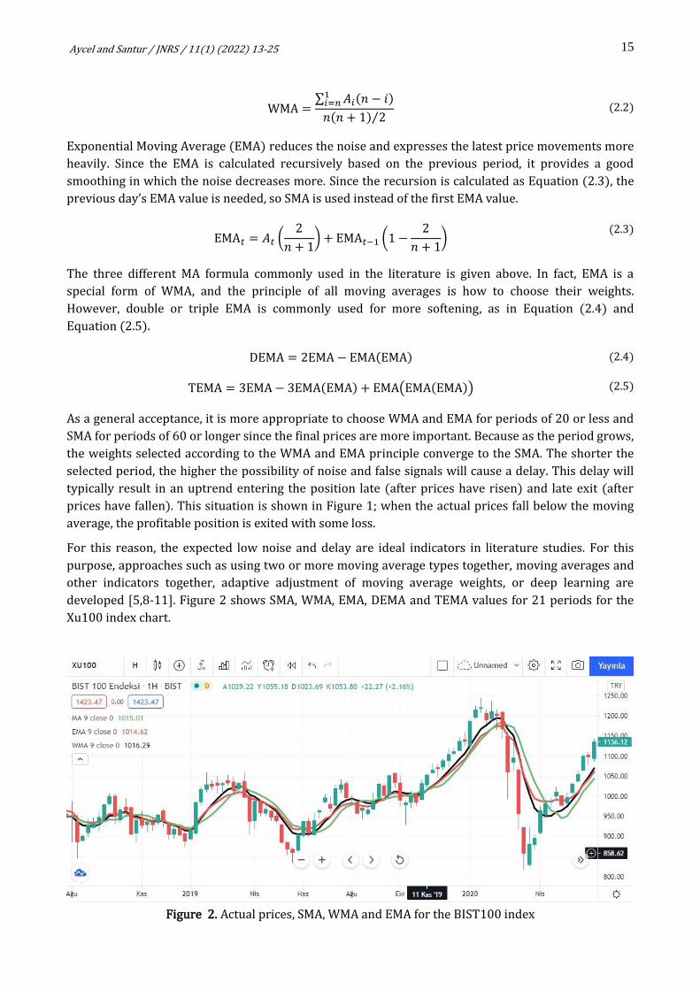
For this reason, the expected low noise and delay are ideal indicators in literature studies. For this

purpose, approaches such as using two or more moving average types together, moving averages and

other indicators together, adaptive adjustment of moving average weights, or deep learning are

developed [5,8-11]. Figure 2 shows SMA, WMA, EMA, DEMA and TEMA values for 21 periods for the

Xu100 index chart.

Figure 2. Actual prices, SMA, WMA and EMA for the BIST100 index

16

Aycel and Santur / JNRS / 11(1) (2022) 13-25

Moving Average Convergence Divergence (MACD) indicator, one of the most popular indicators used

today, is based on the two-period EMA and their softening principle. In Equation (2.6), C denotes the

price closing value. MACDline is the 12 and 26-day EMA difference, respectively, Signalline is a 9-

period smoothing. Histogram shows the difference between these. Accordingly, the MACD strategy is

as follows: If MACDline Signallinecrosses up, it is a “Buy” signal; if it crosses down, it is a “Sell” signal.

Similarly, having the Histogram value below or above 0 is also a strategy. When the upper intersection

is below the Histogram, it is “Weak Buy”; if it is above, it is “Strong Buy”, while the lower intersection is

above the Histogram is “Weak Sell”, and below the Histogram is a “Strong Sell” signal. MACD, which

was successfully applied to Japanese markets in the years it was developed, is still one of the most

widely used and reliable indicators in manual and autonomous systems.

MACDline = EMA(C, 12) − EMA(C, 26)

Signalline = EMA(MACDline, 9)

Histogram = MACDline − Signalline

(2.6)

Another widely used indicator is Bollinger Bands (BB), which consists of three trend lines and takes its

name from the surname of its developer. The middle line is the 20 periods SMA. The upper and lower

bands are obtained by adding and subtracting twice the standard deviation value given in Equation

(2.7) to this middle band. The BB indicator acts with the assumption that the price movements will

move within this band, and the price will return into the band in case of out-of-band.

𝜎 =∑ (𝐴𝑖 − SMA)2𝑛

𝑖=1

𝑛

UpperBand = SMA + 2𝜎

LowerBand = SMA − 2𝜎

(2.7)

Another widely used and compared indicator herein is Relative Strength Index (RSI). In fact, RSI is

used to confirm price extremisms by the indicator in a certain period. In addition, it is normalised to

the 0-100 range and below 30 is considered “Oversold”, and over 70 is considered “Overbought”. In

this case, the indicator is considered to cross over the oversold zone from bottom to top as “Buy”, and

to cross under the overbought zone from top to bottom is regarded as a “Sell” signal. Eq. It is calculated

as in Equation (2.8) and normalised to the 0-100 range. To calculate the RSI value, the RS value is

calculated first. The RS value is obtained by dividing the average of higher closings over the period by

the average of lower closes. As general acceptance, the period value is chosen as 14.

RSI = 100 −100

1 + RS

RS = SMA (U) SMA⁄ (D)

(2.8)

The RSI indicator is one of the most widely used indicators today. However, the aforesaid signals occur

infrequently. Another strategy to be developed using RSI is to compare the current value with its

average. Stochastik RSI (Stoch) works on this principle. The 𝐾% value given in Equation (2.9) is

obtained by normalising the RSI to the 0-1 interval and multiplying it by 100. D% is its 3-day simple

average of the K%. Using Stochastik RSI, when the 𝐾% value crosses over the 𝐷% value up, “Buy” and

when it crosses under down, the “Sell” signal is obtained.

Stoch(K%) = (RSI − min (RSI)) (max(RSI) − min (RSI))⁄

D% = SMA(K%) (2.9)

17

Aycel and Santur / JNRS / 11(1) (2022) 13-25

The last indicator examined in the study is the Parabolic Stop and Reversal (PSAR) indicator. It is used

to catch price and trend changes. Equation (2.10) 𝐶 is the closing price EPT multiplied by the highest

and lowest value of the day for the up and down PSAR, while the AF constant is the constant of 0.2

multiplied by the number of bottoms and peaks of 0.02. As an interpretation, if the current price is

lower than PSAR, it is considered a “Buy”; if it is higher, it is regarded as a “Sell” signal.

PSAR = C + AF(EPT − C) (2.10)

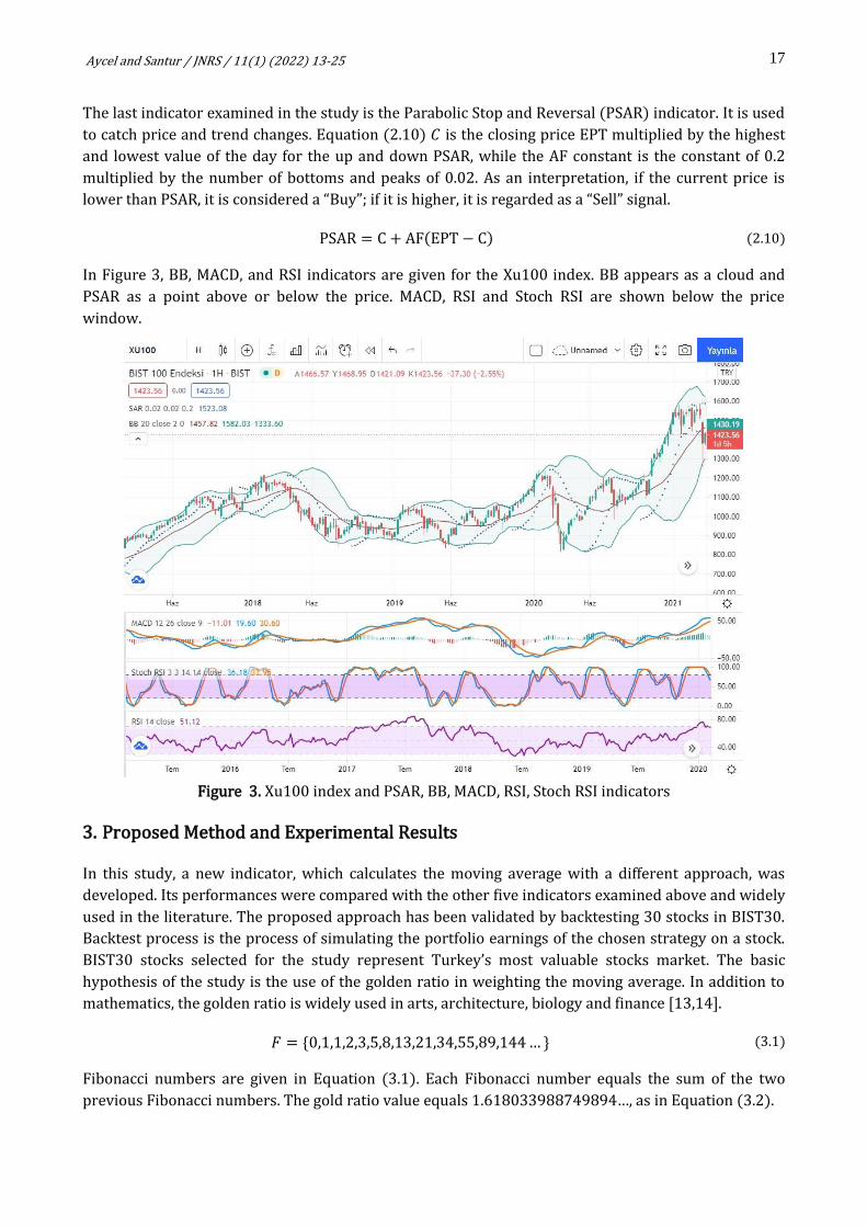
In Figure 3, BB, MACD, and RSI indicators are given for the Xu100 index. BB appears as a cloud and

PSAR as a point above or below the price. MACD, RSI and Stoch RSI are shown below the price

window.

Figure 3. Xu100 index and PSAR, BB, MACD, RSI, Stoch RSI indicators

3. Proposed Method and Experimental Results

In this study, a new indicator, which calculates the moving average with a different approach, was

developed. Its performances were compared with the other five indicators examined above and widely

used in the literature. The proposed approach has been validated by backtesting 30 stocks in BIST30.

Backtest process is the process of simulating the portfolio earnings of the chosen strategy on a stock.

BIST30 stocks selected for the study represent Turkey’s most valuable stocks market. The basic

hypothesis of the study is the use of the golden ratio in weighting the moving average. In addition to

mathematics, the golden ratio is widely used in arts, architecture, biology and finance [13,14].

𝐹 = {0,1,1,2,3,5,8,13,21,34,55,89,144 … } (3.1)

Fibonacci numbers are given in Equation (3.1). Each Fibonacci number equals the sum of the two

previous Fibonacci numbers. The gold ratio value equals 1.618033988749894…, as in Equation (3.2).

18

Aycel and Santur / JNRS / 11(1) (2022) 13-25

𝜙 =1 + √5

2

(3.2)

Dividing two consecutive numbers in the Fibonacci series gives this golden ratio in Equation (3.3).

𝜙 =𝐹𝑛

𝐹𝑛−1 (3.3)

The use of Fibonacci numbers in finance is not an entirely new issue. They are used in price reversals

in changing trends, determining possible support/resistance levels after the horizontal market or

predicting trend periods, fib retracement, trend-based Fibonacci fib time, trend-based fib extension,

fib circles, fib spiral and fib channel [15].

In this study, two different moving averages are calculated using SMA, WMA and EMA by fixing their

weights with the golden ratio. A developed strategy produces buy/sell signals according to the

intersection of these two averages with the price. The work mainly focuses on obtaining a WMA that

uses SMA with gold ratios weights, softening this series with EMA, and optimising it to select the most

suitable parameters for the tested BIST30 stocks. The study was developed using the Pine script

language on the tradingview online platform [16,17]. The value of Fibonacci numbers grows as the

index increases, so multiplying the series by a large number is an issue. Therefore, the first two values

of the W series that make up the weights of the moving average as a constant as in Equation (3.4).

W−1 =1 − √5

2= 0.61803

W0 = 𝜙 − W−1 = 1

W𝑛 = 𝜙𝑛, if 𝑛 > 1

(3.4)

After all, this indicator, experimentally called Trend Follower (TF), is calculated as in Equation (3.5)

and divided by the sum of these preselected weights. Then, the TF value is added to the bias value for

noise reduction.

TF =∑ 𝐴𝑖W𝑖

1𝑖=𝑛

∑ W𝑖

TF = TF(100 + bias) 100⁄

(3.5)

TFsmooth is the 9-period EMA value of the TF value. Similarly, for the noise reduction process. The bias

value is subtracted as in Equation (3.6). As a working principle, as in other indicators, when the TF

value crosses over the value of TFsmooth. A “Buy” signal is generated, and a “Sell” signal is generated

when it crosses down. According to optimisation tests, the W period depth was chosen as 10, the

smoothing value as 9, and bias 0.3.

TFsmooth = EMA(TF, Smooth)

TFsmooth = TFsmooth(100 − bias) 100⁄ (3.6)

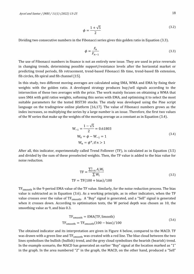
The obtained indicator and its interpretation are given in Figure 4 below, compared to the MACD. TF

was drawn with a green line and TFsmooth was created with a red line. The blue cloud between the two

lines symbolises the bullish (bullish) trend, and the grey cloud symbolises the bearish (bearish) trend.

In the example scenario, the MACD has generated an earlier “Buy” signal at the location marked as “1”

in the graph. In the area numbered “2” in the graph, the MACD, on the other hand, produced a “Sell”

19

Aycel and Santur / JNRS / 11(1) (2022) 13-25

signal that can be regarded as noise but showed that the trend continued in the developed approach,

thereby maintaining the current position. In the place numbered “3” in the graph, an “Buy” signal was

generated earlier than the MACD.

The pseudo-code for the proposed approach’s moving average calculation and backtest phase is as

follows:

Pseudo-code of the proposed approach

train dataset=read (stock, close, high, low, volume, date)

W−1 ⇐ 0.618

W0 ⇐ 1 Depth ⇐ 9 Smooth ⇐ 3 Bias ⇐ 0.3

TF ⇐ 0 Wsum ⇐ 0

while i ≤ Depth do

Wn = ϕn

end while

TF = TF *(100 + bias100 * Wsum)

TFsmooth= EMA(TF)

TFsmooth=TFsmooth (1−bias/100)

#Backtest stage:

i ⇐ 0 while stockdate ≤ Today do

if crossover(Closei, TFsmooth) then

Buy()

end if if crossunder(Closei, TFsmooth) then

Sell()

end if

end while

#Evalutaion portfolio metrics:

PF,GrossProfit,GrossLoss = Backtest()

Figure 4. The indicator, obtained proposed approach in this study, and MACD indicator

Since each stock fluctuates in financial markets, no indicator works ideally. For this reason, to verify

the study, the five indicators and the developed approach were compared for 30 stocks in BIST30 with

the strategy created by coding the pine script language on the tradingview online platform. The

strategy mentioned here involves a portfolio simulating the created Buy / Sell signals to past charts

with an initial default capital. As a result of the simulation, metric values such as net profit obtained

20

Aycel and Santur / JNRS / 11(1) (2022) 13-25

with 100,000 starting capitals in the local currency of the share, profit percentage, number of traded

positions, number of positions closed with profit, and profit coefficient are obtained. The number of

profitable positions and per cent profitable can be quite misleading because short-term positions

frequently opened in the horizontal market have low profits. At the same time, large losses can result

in total portfolio losses. The most optimal comparison is Profit Factor (PF), obtained by dividing gross

profit by gross loss. If this value is less than 1, it indicates that the relevant strategy portfolio is closed

with a loss; if it is greater than 1, it shows that it is closed with profit. Eq. How much the value shown

in Equation (3.7) is greater than 1 varies in proportion to the portfolio gain.

PF =∑ Gross profits

∑ Gross loses (3.7)

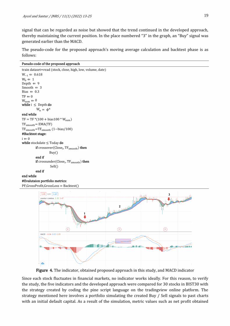
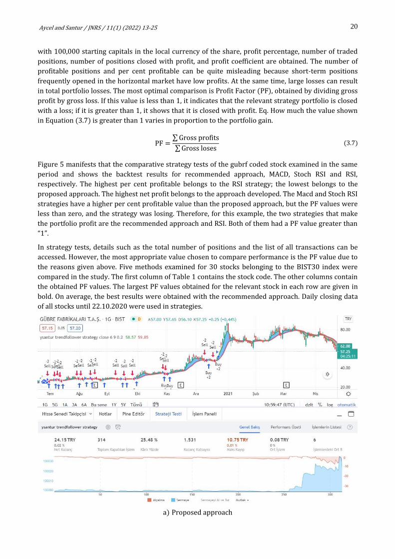
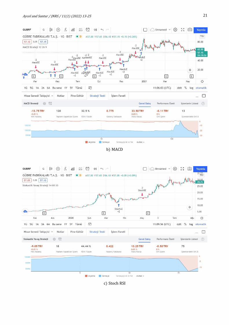
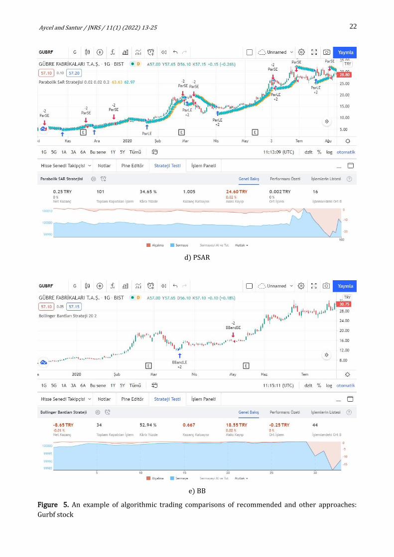
Figure 5 manifests that the comparative strategy tests of the gubrf coded stock examined in the same

period and shows the backtest results for recommended approach, MACD, Stoch RSI and RSI,

respectively. The highest per cent profitable belongs to the RSI strategy; the lowest belongs to the

proposed approach. The highest net profit belongs to the approach developed. The Macd and Stoch RSI

strategies have a higher per cent profitable value than the proposed approach, but the PF values were

less than zero, and the strategy was losing. Therefore, for this example, the two strategies that make

the portfolio profit are the recommended approach and RSI. Both of them had a PF value greater than

“1”.

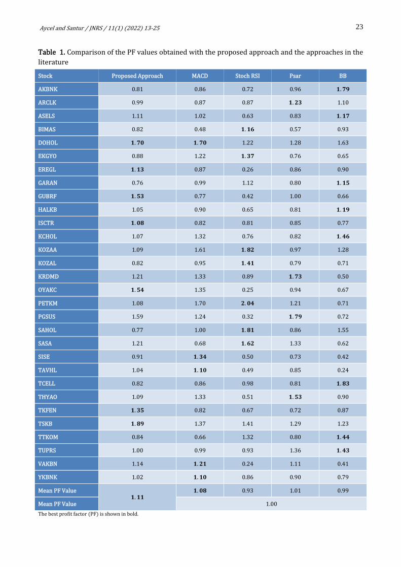
In strategy tests, details such as the total number of positions and the list of all transactions can be

accessed. However, the most appropriate value chosen to compare performance is the PF value due to

the reasons given above. Five methods examined for 30 stocks belonging to the BIST30 index were

compared in the study. The first column of Table 1 contains the stock code. The other columns contain

the obtained PF values. The largest PF values obtained for the relevant stock in each row are given in

bold. On average, the best results were obtained with the recommended approach. Daily closing data

of all stocks until 22.10.2020 were used in strategies.

a) Proposed approach

21

Aycel and Santur / JNRS / 11(1) (2022) 13-25

b) MACD

c) Stoch RSI

22

Aycel and Santur / JNRS / 11(1) (2022) 13-25

d) PSAR

e) BB

Figure 5. An example of algorithmic trading comparisons of recommended and other approaches:

Gurbf stock

23

Aycel and Santur / JNRS / 11(1) (2022) 13-25

Table 1. Comparison of the PF values obtained with the proposed approach and the approaches in the

literature

Stock Proposed Approach MACD Stoch RSI Psar BB

AKBNK 0.81 0.86 0.72 0.96 𝟏. 𝟕𝟗

ARCLK 0.99 0.87 0.87 𝟏. 𝟐𝟑 1.10

ASELS 1.11 1.02 0.63 0.83 𝟏. 𝟏𝟕

BIMAS 0.82 0.48 𝟏. 𝟏𝟔 0.57 0.93

DOHOL 𝟏. 𝟕𝟎 𝟏. 𝟕𝟎 1.22 1.28 1.63

EKGYO 0.88 1.22 𝟏. 𝟑𝟕 0.76 0.65

EREGL 𝟏. 𝟏𝟑 0.87 0.26 0.86 0.90

GARAN 0.76 0.99 1.12 0.80 𝟏. 𝟏𝟓

GUBRF 𝟏. 𝟓𝟑 0.77 0.42 1.00 0.66

HALKB 1.05 0.90 0.65 0.81 𝟏. 𝟏𝟗

ISCTR 𝟏. 𝟎𝟖 0.82 0.81 0.85 0.77

KCHOL 1.07 1.32 0.76 0.82 𝟏. 𝟒𝟔

KOZAA 1.09 1.61 𝟏. 𝟖𝟐 0.97 1.28

KOZAL 0.82 0.95 𝟏. 𝟒𝟏 0.79 0.71

KRDMD 1.21 1.33 0.89 𝟏. 𝟕𝟑 0.50

OYAKC 𝟏. 𝟓𝟒 1.35 0.25 0.94 0.67

PETKM 1.08 1.70 𝟐. 𝟎𝟒 1.21 0.71

PGSUS 1.59 1.24 0.32 𝟏. 𝟕𝟗 0.72

SAHOL 0.77 1.00 𝟏. 𝟖𝟏 0.86 1.55

SASA 1.21 0.68 𝟏. 𝟔𝟐 1.33 0.62

SISE 0.91 𝟏. 𝟑𝟒 0.50 0.73 0.42

TAVHL 1.04 𝟏. 𝟏𝟎 0.49 0.85 0.24

TCELL 0.82 0.86 0.98 0.81 𝟏. 𝟖𝟑

THYAO 1.09 1.33 0.51 𝟏. 𝟓𝟑 0.90

TKFEN 𝟏. 𝟑𝟓 0.82 0.67 0.72 0.87

TSKB 𝟏. 𝟖𝟗 1.37 1.41 1.29 1.23

TTKOM 0.84 0.66 1.32 0.80 𝟏. 𝟒𝟒

TUPRS 1.00 0.99 0.93 1.36 𝟏. 𝟒𝟑

VAKBN 1.14 𝟏. 𝟐𝟏 0.24 1.11 0.41

YKBNK 1.02 𝟏. 𝟏𝟎 0.86 0.90 0.79

Mean PF Value 𝟏. 𝟏𝟏

𝟏. 𝟎𝟖 0.93 1.01 0.99

Mean PF Value 1.00

The best profit factor (PF) is shown in bold.

24

Aycel and Santur / JNRS / 11(1) (2022) 13-25

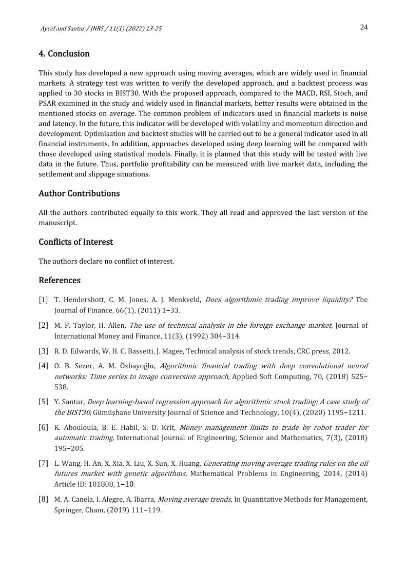
4. Conclusion

This study has developed a new approach using moving averages, which are widely used in financial

markets. A strategy test was written to verify the developed approach, and a backtest process was

applied to 30 stocks in BIST30. With the proposed approach, compared to the MACD, RSI, Stoch, and

PSAR examined in the study and widely used in financial markets, better results were obtained in the

mentioned stocks on average. The common problem of indicators used in financial markets is noise

and latency. In the future, this indicator will be developed with volatility and momentum direction and

development. Optimisation and backtest studies will be carried out to be a general indicator used in all

financial instruments. In addition, approaches developed using deep learning will be compared with

those developed using statistical models. Finally, it is planned that this study will be tested with live

data in the future. Thus, portfolio profitability can be measured with live market data, including the

settlement and slippage situations.

Author Contributions

All the authors contributed equally to this work. They all read and approved the last version of the

manuscript.

Conflicts of Interest

The authors declare no conflict of interest.

References

[1] T. Hendershott, C. M. Jones, A. J. Menkveld, Does algorithmic trading improve liquidity? The

Journal of Finance, 66(1), (2011) 1–33.

[2] M. P. Taylor, H. Allen, The use of technical analysis in the foreign exchange market, Journal of

International Money and Finance, 11(3), (1992) 304–314.

[3] R. D. Edwards, W. H. C. Bassetti, J. Magee, Technical analysis of stock trends, CRC press, 2012.

[4] O. B. Sezer, A. M. Özbayoğlu, Algorithmic financial trading with deep convolutional neural

networks: Time series to image conversion approach, Applied Soft Computing, 70, (2018) 525–

538.

[5] Y. Santur, Deep learning-based regression approach for algorithmic stock trading: A case study of

the BIST30, Gümüşhane University Journal of Science and Technology, 10(4), (2020) 1195–1211.

[6] K. Abouloula, B. E. Habil, S. D. Krit, Money management limits to trade by robot trader for

automatic trading, International Journal of Engineering, Science and Mathematics, 7(3), (2018)

195–205.

[7] L. Wang, H. An, X. Xia, X. Liu, X. Sun, X. Huang, Generating moving average trading rules on the oil

futures market with genetic algorithms, Mathematical Problems in Engineering, 2014, (2014)

Article ID: 101808, 1–10.

[8] M. A. Canela, I. Alegre, A. Ibarra, Moving average trends, In Quantitative Methods for Management,

Springer, Cham, (2019) 111–119.

25

Aycel and Santur / JNRS / 11(1) (2022) 13-25

[9] O. B. Sezer, M. U. Güdelek, A. M. Özbayoğlu, Financial time series forecasting with deep learning: A

systematic literature review: 2005–2019, Applied Soft Computing, 90, (2020) 106181.

[10] A. M. Ozbayoglu, M. U. Gudelek, O. B. Sezer, Deep learning for financial applications: A survey,

Applied Soft Computing, 93, (2020) 106384, 1–29.

[11] E. León-Castro, E. Avilés-Ochoa, J. M. Merigó, A. M. Gil-Lafuente, Heavy moving averages and their

application in econometric forecasting, Cybernetics and Systems, 49(1), (2018) 26–43.

[12] S. Siami-Namini, N. Tavakoli, A. S. Namin, A comparative analysis of forecasting financial time

series using ARIMA, LSTM, and BILSTM, arXiv preprint arXiv:1911.09512, (2019).

[13] R. J. Bauer, J. R. Dahlquist, Technical Markets Indicators: Analysis & Performance (Vol. 64), John

Wiley & Sons, 1998.

[14] N. Gabdrakhmanova, V. Fedin, B. Matsuta, M. Pilgun, The modeling of forecasting new situations in

the dynamics of the economic system on the example of several financial indicators, Procedia

Computer Science, 186, (2021) 512–520.

[15] L. Lusindah, E. Sumirat, Implementation of Fibonacci Retracements and Exponential Moving

Average (EMA) Trading Strategy in Indonesia Stock Exchange, European Journal of Business and

Management Research, 6(4), (2021) 402–408.

[16] TradingView, Web services for traders, is the most popular technical analysis support platform,

(2021), https://www.tradingview.com

[17] TradingView pine script 4 user manuel, (2021), https://www.tradingview.com/pine-script-

docs/en/v4/index.html