A New Monte Carlo Approach for Conservation Laws and Relaxation Systems

A New Monte Carlo Approach for ConservationLaws and Relaxation Systems

Lorenzo Pareschi1 and Mohammed Seaıd2

1 Department of Mathematics, University of Ferrara, 44100 [email protected]

2 Fachbereich Mathematik AG8, TU Darmstadt, 64289 Darmstadt, [email protected]

Abstract. We present a Monte Carlo method for approximating thesolution of conservation laws. A relaxation method is used to transformthe conservation law to a kinetic form that can be interpreted in a prob-abilistic manner. A Monte Carlo algorithm is then used to simulate thekinetic approximation. The method we present in this paper is simpleto formulate and to implement, and can be straightforwardly extendedto higher dimensional conservation laws. Numerical experiments are car-ried out using Burgers equation subject to both smooth and nonsmoothinitial data.

1 Introduction

Monte Carlo methods have been always very popular in scientific computing.This is mainly due to the ability to deal efficiently with very large (multiscale)structures without many meshing problems and to their simplicity in keepingthe fundamental physical properties of the problems. In particular Monte Carlomethods have been widely used for numerical simulations in rarefied gas dynam-ics described by the Boltzmann equation [1, 5]. More recently these methodshave been extended to treat regimes close to continuum situations described bythe Euler or Navier-Stokes equations [7–9, 2]. The common idea in these approx-imations is to take advantage of the knowledge of the equilibrium state of theequation to build a scheme with the correct behavior close to the fluid-limit. Forexample, for the Boltzmann equation close to fluid regimes particles are sampleddirectly from a Maxwellian distribution as in Pullin’s method [10]. In this arti-cle, inspired by these methods, we use a relaxation approximation to transforma conservation law into a semilinear system which has the structure of a discretevelocity model of the Boltzmann equation. This kinetic form leads naturally to aprobabilistic representation. Therefore, the main ideas used in [7–9] can be usedto simulate the limiting conservation law. More precisely advection of particlesis made according to the characteristic speeds of the relaxation system, andthe projection into the local equilibrium is performed with a suitable samplingstrategy.

2 Lorenzo Pareschi et al.

Let consider the scalar conservation law

ut + ϕ(u)x = 0, (x, t) ∈ R× R+,(1)

u(x, t = 0) = u0(x), x ∈ R,

where u ∈ R and the flux function ϕ(u) : R → R is nonlinear. As in [3], wereplace the scalar Cauchy problem (1) by the semilinear relaxation system

ut + vx = 0,

vt + aux = −1ε

(v − ϕ(u)) , (2)

u(x, 0) = u0(x), v(x, 0) = ϕ (u0(x)) ,

where v ∈ R, a is positive constant, and ε is the relaxation rate. When ε −→ 0,solution of the relaxation system (2) approaches solution of the original equation(1) by the local equilibrium v = ϕ(u). A necessary condition for such convergenceis that the subcharacteristic condition [3, 6]

−a ≤ ϕ′(u) ≤ a, ∀ u, (3)

is satisfied in (2). The main advantage in considering the relaxation method liesessentially on the semilinear structure of the system (2), which has two linearcharacteristic variables (given by v ± √au), and consequently it can be solvednumerically without using Riemann solvers (see [3] and the references therein).

Our purpose in the present paper is to construct a Monte Carlo approachfor the conservation law (1) using the fact that, for the relaxation system (2)a kinetic formulation can be easily derived. The organization of the paper is asfollows. Section 2 is devoted to the probabilistic formulation for the relaxationsystem (2). In section 3 we discuss a Monte Carlo algorithm for the relaxationmodel. Section 4 illustrates the performance of the approach through experi-ments with the Burgers equation. In the last section some concluding remarksand future developments are listed.

2 Probabilistic Interpretation

In order to develop a probabilistic formulation for the relaxation system (2) weintroduce the kinetic variables f and g as

u = f + g and v = a(f − g). (4)

The relaxation system can be rewritten in a diagonal form as

ft +√

afx =1ε

(g − f

2+

ϕ(f + g)2√

a

),

(5)

gt −√

agx =1ε

(f − g

2− ϕ(f + g)

2√

a

).

A Monte Carlo Relaxation Approach 3

To solve numerically the equations (5) we split the problem into two steps:(i) The transport stage

ft +√

afx = 0,(6)

gt −√

agx = 0.

(ii) The relaxation stage

ft =1ε

(g − f

2+

ϕ(f + g)2√

a

),

(7)

gt =1ε

(f − g

2− ϕ(f + g)

2√

a

).

Note that this splitting is first order accurate. A second order splitting for moder-ately stiff relaxation stages can be derived analogously using the Strang method[11]. For simplicity first we will describe the relaxation problem (7), and thenwe show how to combine it with the stage (6) for the full problem.

We assume, without loss of generality, that for a fixed x

f ≥ 0, g ≥ 0, u = f + g = 1.

Furthermore, we assume that the flux function in (1) satisfies

ϕ′(u) < 1, 0 ≤ ϕ(u) ≤ u. (8)

Although problem (7) can be solved exactly we consider its time discretization

fn+1 = fn +∆t

ε

(gn+1 − fn+1

2+

ϕ(fn+1 + gn+1)2

),

(9)

gn+1 = gn +∆t

ε

(fn+1 − gn+1

2− ϕ(fn+1 + gn+1)

2

).

Since fn+1 + gn+1 = fn + gn we can write

fn+1 = fn +∆t

ε

(ε

ε + ∆t

gn+1 − fn+1

2+

ε

ε + ∆t

ϕ(fn+1 + gn+1)2

),

gn+1 = gn +∆t

ε

(ε

ε + ∆t

fn+1 − gn+1

2− ε

ε + ∆t

ϕ(fn+1 + gn+1)2

).

Or equivalently

fn+1 = (1− λ)fn + λ

(gn+1 − fn+1

2+

ϕ(fn+1 + gn+1)2

),

(10)

gn+1 = (1− λ)gn + λ

(fn+1 − gn+1

2− ϕ(fn+1 + gn+1)

2

),

4 Lorenzo Pareschi et al.

with λ =ε

ε + ∆t. Now let us define the probability density

Pn(ξ) =

fn, if ξ = +√

a,

gn, if ξ = −√a,

0, elsewhere.

Note that 0 ≤ Pn(ξ) ≤ 1 and∑

ξ Pn(ξ) = 1. Moreover

∑

ξ

Pn+1(ξ) =∑

ξ

Pn(ξ) = 1.

The system (10) can be seen as the evolution of the probability function Pn(ξ)according with

Pn+1(ξ) =

(1− λ)fn + λEf (un), if ξ = +√

a,

(1− λ)gn + λEg(un), if ξ = −√a,

0, elsewhere,(11)

where Ef (u) =u + ϕ(u)

2and Eg(u) =

u− ϕ(u)2

.

We remark that, since ε > 0, the condition 0 ≤ λ ≤ 1 is satisfied. Obviously,(11) represents a convex combination of two probability densities. In fact, thanksto (8), we have Ef (u) ≥ 0, Eg(u) ≥ 0 and Ef (u) + Eg(u) = 1.

3 Monte Carlo Algorithm

In order to develop a Monte Carlo game to approach the solution to the kineticsystem (5), in addition to a good random number generator, we need a wayto sample particles from an initial data and some other basic tools which aredescribed with details in the lecture notes [9]. Thus, we consider two families ofparticles that defines samples of our probability density Pn(ξ).

Let us define with {ξ1, ξ2, . . . , ξN} the particle samples, we know that ξj =+√

a or ξj = −√a with probability fn or gn respectively. We have the relation

Pn+1(ξ) = (1− λ)Pn(ξ) + λEn(ξ), (12)

where En(ξ) is defined as: En(ξ) =

u + ϕ(u)2

, if ξ = +√

a,

u− ϕ(u)2

, if ξ = −√a,

0, elsewhere.Hence, the relaxation stage (7) can be solved in the following way:

• Given a particle sample ξ the evolution of the sample during the time inte-gration process is performed according to :◦ with probability (1− λ) the sample is unchanged

A Monte Carlo Relaxation Approach 5

◦ with probability λ the sample is replaced with a sample from En(ξ)• To sample a particle from En(ξ) we proceed as follows:

◦ with probabilityu + ϕ(u)

2take ξ = +

√a

◦ with probabilityu− ϕ(u)

2take ξ = −√a

Note that the relaxation stage is well defined for any value of ε. In particular asε → 0 we have λ → 1 and thus particles are all sampled from the local equilib-rium En(ξ). To generate particles the spatial domain is first divided into cells[xi− 1

2, xi+ 1

2] with stepsize ∆x and centered in xi. Then particles are generated

from a given piecewise initial data in each cell and are randomly distributedaround the cell center xi.

Once the particle distribution is updated by the above steps, the transportstage (6) of the splitting is realized by advecting the position of the particlesaccording to their speeds. Thus, given a sample of N particles at positionsx1, x2, · · · , xN and speeds ξ1, ξ2, · · · , ξN (equal either to +

√a or −√a) the new

position of the particle sample {xi, ξi} is simply

xnewi = xold

i + ∆tξi, i = 1, . . . , N,

where xnewi and xold

i are respectively, the new and old positions of the sampleξi, and ∆t is the time stepsize.

Remark 1 The Monte Carlo method presented in this paper applies also if u > 0and u 6= 1. For this case

Pn(ξ) =

fn

un, if ξ = +

√a,

gn

un, if ξ = −√a,

0, elsewhere.

and En(ξ) =

u + ϕ(u)2u

, if ξ = +√

a,

u− ϕ(u)2u

, if ξ = −√a,

0, elsewhere.

It is easy to verify that in this case, Pn defines a probability (i.e., 0 ≤ Pn(ξ) ≤ 1and

∑ξ Pn(ξ) = 1).

4 Numerical Results

In what follows we present numerical results obtained for some tests on Burgersequation given by the equation (1) with the flux function defined as ϕ(u) = u2

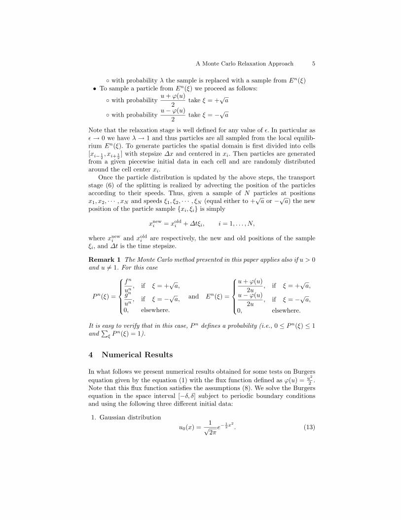
2 .Note that this flux function satisfies the assumptions (8). We solve the Burgersequation in the space interval [−δ, δ] subject to periodic boundary conditionsand using the following three different initial data:

1. Gaussian distributionu0(x) =

1√2π

e−12 x2

. (13)

6 Lorenzo Pareschi et al.

2. Box distribution

u0(x) =

2δ, if |x| ≤ δ

4,

0, elsewhere.(14)

3. Cone distribution

u0(x) =

−4|x|

δ2+

2δ, if |x| ≤ δ

2,

0, elsewhere.(15)

Note that the total mass in these initial data is equal to unity,∫R u0(x)dx = 1.

In all our computations we used δ = 5, the spatial interval is discretized intoM = 100 gridpoints uniformly spaced. The number of particles N is set to 104

which is large enough to decrease the effect of the fluctuations in the computedsolutions. Here we present only results for the relaxed case (i.e. ε = 0). Resultsfor the relaxing case (i.e. ε 6= 0) can be done analogously. The time step ∆t ischosen such a way the CFL = 1 and the computation have been performed witha single run for different time t ∈ [0, 10].

02

46

810

−5 −4 −3 −2 −1 0 1 2 3 4 5

0

0.05

0.1

0.15

0.2

0.25

0.3

0.35

0.4

0.45

0.5

xt

u

02

46

810

−5 −4 −3 −2 −1 0 1 2 3 4 5

0

0.05

0.1

0.15

0.2

0.25

0.3

0.35

0.4

0.45

0.5

xt

u

02

46

810

−5 −4 −3 −2 −1 0 1 2 3 4 5

0

0.05

0.1

0.15

0.2

0.25

0.3

0.35

0.4

0.45

0.5

xt

u

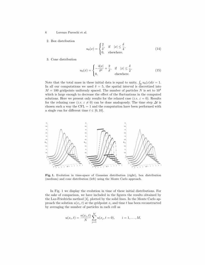
Fig. 1. Evolution in time-space of Gaussian distribution (right), box distribution(medium) and cone distribution (left) using the Monte Carlo approach.

In Fig. 1 we display the evolution in time of these initial distributions. Forthe sake of comparison, we have included in the figures the results obtained bythe Lax-Friedrichs method [4], plotted by the solid lines. In the Monte Carlo ap-proach the solution u(xi, t) at the gridpoint xi and time t has been reconstructedby averaging the number of particles in each cell as

u(xi, t) =n(xi, t)

N

M∑

j=1

u(xj , t = 0), i = 1, . . . , M,

A Monte Carlo Relaxation Approach 7

where n(xi, t) denotes the number of the particles localized in the cell [xi− 12, xi+ 1

2]

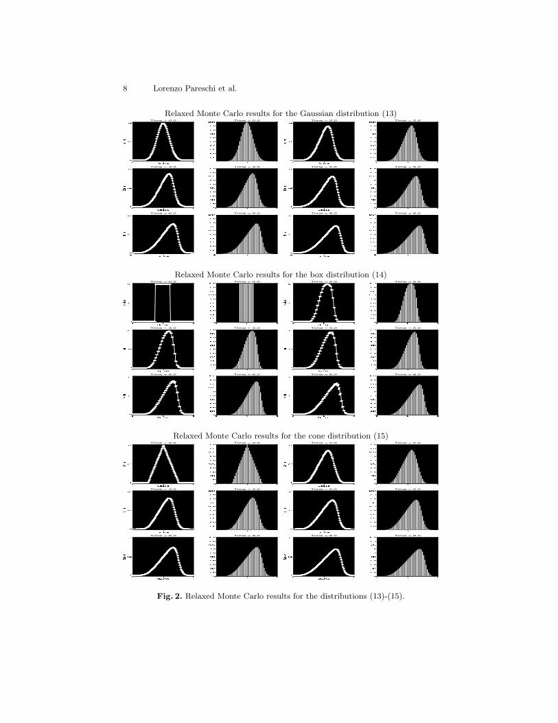
at time t. As can be seen the shock is well captured by the Monte Carlo method.Fig. 2 shows again the results for the initial data (13)-(15) along with the evo-lution of particle distribution in the space interval for six different times. TheMonte Carlo approach preserves the positivity of the solution as well as theconservation of mass

∫

Ru(x, t)dx =

∫

Ru0(x)dx = 1, ∀ t > 0.

We would like to mention that the new Monte Carlo approach can approximateconservation laws with diffusive source terms, for example viscous Burgers equa-tions. The diffusion stage in the algorithm can be treated, for example, by thewell-known Random walk method.

5 Concluding Remarks

We have presented a simple Monte Carlo algorithm for the numerical solutionof conservation laws and relaxation systems. The algorithm takes advantage ofthe relaxation model associated to the equation under consideration which canbe regarded as the evolution in time of a probability distribution. Although wehave restricted our numerical computations to the case of one-dimensional scalarproblems, the most important implication of our research concerns the use ofeffective Monte Carlo procedures for multi-dimensional systems of conservationlaws with relaxation terms similarly to the Broadwell system and the BGK modelin rarefied gas dynamics. Our current effort is therefore to extend this approachto systems of conservation laws in higher space dimensions. Another extensionwill be to couple the Monte Carlo method at the large ε scale with a deterministicmethod at the reduced small ε scale as in [2] for a general relaxation system.Finally we remark that the Monte Carlo approach proposed in this paper isrestricted to first order accuracy. A second order method it is actually understudy.

Acknowledgements. The work of the second author was done during a visitat Ferrara university. The author thanks the department of mathematics for thehospitality and for technical and financial support. Support by the Europeannetwork HYKE, funded by the EC as contract HPRN-CT-2002-00282, is alsoacknowledged.

References

1. Bird G.A.: Molecular Gas Dynamics. Oxford University Press, London, (1976)2. Caflisch R.E., Pareschi L.: An implicit Monte Carlo Method for Rarefied Gas Dy-

namics I: The Space Homogeneous Case. J. Comp. Physics 154 (1999) 90–1163. Jin S., Xin, Z.: The Relaxation Schemes for Systems of Conservation Laws in

Arbitrary Space Dimensions. Comm. Pure Appl. Math. 48 (1995) 235–276

8 Lorenzo Pareschi et al.

Relaxed Monte Carlo results for the Gaussian distribution (13)

Relaxed Monte Carlo results for the box distribution (14)

Relaxed Monte Carlo results for the cone distribution (15)

Fig. 2. Relaxed Monte Carlo results for the distributions (13)-(15).

A Monte Carlo Relaxation Approach 9

4. LeVeque Randall J.: Numerical Methods for Conservation Laws. Lectures in Math-ematics ETH Zurich, (1992)

5. Nanbu K.: Direct Simulation Scheme Derived from the Boltzmann Equation. J.Phys. Soc. Japan, 49 (1980) 2042–2049

6. Natalini, R.: Convergence to Equilibrium for Relaxation Approximations of Con-servation Laws. Comm. Pure Appl. Math. 49 (1996) 795–823

7. Pareschi L., Wennberg B.: A Recursive Monte Carlo Algorithm for the BoltzmannEquation in the Maxwellian Case. Monte Carlo Methods and Applications 7 (2001)349–357

8. Pareschi L., Russo G.: Time Relaxed Monte Carlo Methods for the BoltzmannEquation. SIAM J. Sci. Comput. 23 (2001) 1253–1273

9. Pareschi L., Russo G.: An Introduction to Monte Carlo Methods for the BoltzmannEquation. ESAIM: Proceedings 10 (2001) 35–75

10. Pullin D.I.: Generation of Normal Variates with Given Sample. J. Statist. Comput.Simulation 9 (1979) 303–309

11. Strang, G.: On the Construction and the Comparison of Difference Schemes. SIAMJ. Numer. Anal. 5 (1968) 506–517