A New Method for Analyzing Sequential Processes: Dynamic Multilevel Analysis

http://sgr.sagepub.comSmall Group Research

DOI: 10.1177/1046496405279309 2005; 36; 600 Small Group Research

Ming Ming Chiu and Lawrence Khoo A New Method for Analyzing Sequential Processes: Dynamic Multilevel Analysis

http://sgr.sagepub.com/cgi/content/abstract/36/5/600 The online version of this article can be found at:

Published by:

http://www.sagepublications.com

can be found at:Small Group Research Additional services and information for

http://sgr.sagepub.com/cgi/alerts Email Alerts:

http://sgr.sagepub.com/subscriptions Subscriptions:

http://www.sagepub.com/journalsReprints.navReprints:

http://www.sagepub.com/journalsPermissions.navPermissions:

http://sgr.sagepub.com/cgi/content/refs/36/5/600 Citations

at CHINESE UNIV HONG KONG LIB on June 19, 2009 http://sgr.sagepub.comDownloaded from

http://sgr.sagepub.com/cgi/alerts

http://sgr.sagepub.com/subscriptions

http://www.sagepub.com/journalsReprints.nav

http://www.sagepub.com/journalsPermissions.nav

http://sgr.sagepub.com/cgi/content/refs/36/5/600

http://sgr.sagepub.com

10.1177/1046496405279309SMALL GROUP RESEARCH / October 2005Chiu, Khoo / ANALYZING SEQUENTIAL PROCESSES

A NEW METHOD FOR ANALYZINGSEQUENTIAL PROCESSES:

Dynamic Multilevel Analysis

MING MING CHIUChinese University of Hong Kong

LAWRENCE KHOOCity University of Hong Kong

Researchers studying sequential processes (e.g., marital conflicts, teacher-student interac-tions, etc.) often try to model how recent events affect current events. A researcher doing sofaces several difficulties: the threat of combinatorial explosion due to comprehensive coding,continuous and discrete variables, and differences across time (nonstationarity) and acrossgroups (group heterogeneity). The authors discuss three often-used methods of analyzingtime-series data (conditional probabilities, sequential analysis, and Logit with lag vari-ables) and the problems inherent in them. The authors then introduce a new method thataddresses the above problems: dynamic multilevel analysis. To highlight the similarities anddifferences between these methods, the authors apply them to data from student group prob-lem-solving sessions in an algebra class. The authors use the various methods to show howlikelihood of agreement was affected by other recent speakers’ correct ideas, mathematicsstatus, agreement, and rudeness.

Keywords: social interaction; sequential analysis; time-series analysis

Many phenomena are inherently sequential. When analyzingseries of sequential events (or time-series data), researchers oftenmodel how events are affected by recent events within a series.Examples include student interactions with other students or with

600

AUTHORS’ NOTE: This research was partially funded by a National Academy of Educa-tion/Spencer Foundation postdoctoral fellowship, a Spencer Foundation research grant, anda Chinese University of Hong Kong direct grant. We appreciate Choi Yik Ting’s researchassistance. An earlier version of this article was presented at the annual meeting of the Amer-ican Educational Research Association in New Orleans, Louisiana, in 2002.

SMALL GROUP RESEARCH, Vol. 36 No. 5, October 2005 600-631DOI: 10.1177/1046496405279309© 2005 Sage Publications



Karolina Lisiecka

Karolina Lisiecka

Karolina Lisiecka

Karolina Lisiecka

teachers (Chiu, 2004; Chiu & Khoo, 2003), marital conflict(Gottman et al., 2003), and preschoolers’ play (Farran & Son-Yarbrough, 2001). Consider a group of people discussing how tosolve a problem. Each person’s action might affect later actions byother group members. For example, a person who states a correctidea likely raises the probability that the next person agrees. Thisexample is a special case of the general phenomenon of a series ofinteractions among two or more entities (people, animals, coun-tries, etc.).

In this article, we consider the general class of phenomena ofcurrent events being affected by recent past events (and also bynon-time-dependent characteristics). We examine the difficultiesinvolved in modeling time-series data and several methods fordoing so. To concretize the methodological issues, we introduce aspecific set of hypotheses and a data set. Then we consider threetypes of difficulties in analyzing time-series data: coding difficul-ties, lack of independence among the observations, and heteroge-neity in the data set. Next, we review past methods used to modeltime-series data: conditional probabilities, sequential analysis, andLogit. We then introduce a new method that we call dynamic multi-level analysis (DMA, based in part on Chiu, 2000) and discuss howit mitigates these difficulties. To illustrate the differences amongthese methods, we use all of them on one data set to test severalresearch hypotheses. We then conclude with a comparison of thevarious methods.

Before we proceed further, we wish to introduce some terminol-ogy. The sequential processes we discuss can involve groups,dyads, or individuals. To avoid confusion, we refer to the objectunder study (group, dyad, or individual) as the sampling unit. Asampling unit can be observed on one or more occasions; we referto each such occasion as a session. If warranted, we can furtherdivide each session into time periods. During a session, we observea stream of sequential behavior. Before analysis, coders parse thisstream of sequential behavior into discrete behaviors. We refer toeach such discrete behavior as a turn. Often, coders further assigneach discrete behavior to one of a set of categories, categorizing thenature of each turn.

Chiu, Khoo / ANALYZING SEQUENTIAL PROCESSES 601



EXAMPLE OFTIME-SERIES DATA AND HYPOTHESES

We begin with a specific set of data and hypotheses drawn fromChiu and Khoo (2003) to contextualize the methodological issuesinvolved. Later, we test these hypotheses by applying all of the vari-ous methods to this data.

DATA

The data consist of 80 middle school students’ grades and tran-scribed videotapes. These students worked on an algebra wordproblem in 20 groups of 4 students each. The sampling unit for thisstudy is the group. Each group was videotaped for one session. Thesmallest unit of analysis is a speaker’s turn in a group’s conversa-tion. The transcribed videotapes included 3,104 speaker turns ofconversation. Distinct time periods might exist within each session,forming an intermediate level of analysis.

Two research assistants who were unaware of the researchhypotheses coded each speaker turn for the following: correctness,speaker’s mathematics status, and evaluation of the previousspeaker. A speaker’s mathematics status was computed as his or hermathematics grade minus his or her group’s mean mathematicsgrade. Evaluations included agreement, polite disagreement,impolite disagreement, neutral actions, and an ignoring of the pre-vious speaker. So the analysis included discrete variables—correct,agree, rudely disagree, and ignore—and a continuous variable,math status. We used Cohen’s (1960) kappa to test for interraterreliability.

HYPOTHESES

In an ideal world, a person agrees when the previous speakerstates a correct idea and disagrees otherwise. However, other fac-tors such as status, politeness, and recent agreements might alsoaffect agreement. Controlling for correctness, the previousspeaker’s past achievements relative to those of other group mem-

602 SMALL GROUP RESEARCH / October 2005



bers (achievement status) may also affect others’evaluations of hisor her idea. Thus, past mathematics grades might bias agreementwhen a group works on a mathematics problem. Also, rude actionssuch as ignoring the previous speaker and disagreeing rudely mightcause other group members to become defensive and hence lesslikely to agree with the rude person. Finally, agreement in recentturns may also predict future agreement because previous agree-ments are likely to build a common knowledge base for agreementin the following turns.

We predict the outcome variable of agree with both turn-levelvariables and individual-level variables. All turn-level explanatoryvariables occur before the turn of the outcome variable. Therefore,time constrains the direction of causality. Restating these hypothe-ses in terms of the variables, we have the following (time lags are inparentheses; –1 indicates the previous turn):

• Previous speaker’s correctness predicts agreement: Correct(–1 . . . –4; up to four turns ago), correctness of the previous speaker,positively predicts agree (0), agreement by the current speaker.

• Previous speaker’s achievement status predicts agreement: Mathstatus (–1 . . . –4) positively predicts agree (0).

• Previous speakers’ rude disagreements negatively predict agree-ment: Rudely disagree (–1 . . . –4) negatively predicts agree (0).

• Being ignored negatively predicts agreement: Ignore (–1 . . . –4)negatively predicts agree (0).

• Agreement in recent turns predicts agreement: Agree (–1 . . . –4)positively predicts agree (0).

DIFFICULTIES INANALYZING TIME-SERIES DATA

Methods for analyzing time-series data must address at leastthree types of difficulties: coding difficulties, lack of independenceamong the observations, and heterogeneity. First, sophisticatedhypotheses often require intricate coding of behaviors that threatenconsistency and reliability. Second, time-series data observed fromdifferent individuals or groups usually violate the independenceassumption of many statistics methods. Last, the effect of the




explanatory variables on the outcome variable can differ acrossgroups (group heterogeneity) or change over time (time period het-erogeneity or nonstationarity).

CODING DIFFICULTIES

The usefulness of any statistical analysis depends, in part, on thequality of the coding scheme. Ideally, a coding framework for sta-tistical analyses has mutually exclusive and exhaustive categories.Furthermore, these categories should be sufficiently comprehen-sive to test one’s hypotheses.

However, a complex coding scheme with mutually exclusiveand exhaustive categories often includes many codes (e.g., Chiu,2000). As the number and complexity of the hypotheses rise, thenumber of codes also rises. This increases the complexity of thecoding schemes, the training time for coders, the coding time, andcoding conflicts. Thus, complex coding schemes can reduce inter-nal consistency and intercoder reliability.

Moreover, coding schemes with a large number of categoriescan be statistically problematic. Models with many variables canreduce the available degrees of freedom and the precision of param-eter estimates.

NONINDEPENDENT OBSERVATIONS

Researchers studying sequential processes often find that theirdata violate the assumptions required by traditional statistical mod-els. Methods such as ordinary least squares assume that the modelerrors are independent between observations (Judge, Griffiths,Hill, Lutkepohl, & Lee, 1985). This assumption is violated by thenature of sequential (or time-series) data, because observations areusually affected by other recent observations. This assumption isalso violated when sequential observations are drawn from differ-ent sampling units. Observations within a sampling unit can resem-ble one another substantially and differ from those in other groupsin unobserved ways. Ignoring the nonindependence of the observa-




tions can lead to inefficient effect-size estimates and biased esti-mates of the significance of the explanatory variables.

GROUP HETEROGENEITY AND NONSTATIONARITY

Traditional models also assume that explanatory variable effectsare stable over the entire data set. However, this assumption is oftenviolated, because explanatory variable effects can differ acrosssampling units (also known as group heterogeneity; Goodman,Ravlin, & Schminke, 1987) and also across time (nonstationarity);Dabbs & Ruback, 1987; Goodman et al., 1987). Consider data withmultiple sampling units, specifically pairs of students. The inter-actions between one pair of students can differ substantially fromthose of other pairs of students. To model these interactions accu-rately, we need different parameter estimates for each samplingunit.

The effect of an explanatory variable might also change overtime. For example, people may agree more often at the end of aproblem-solving session than at the beginning of one. They mightdisagree regularly until they find a correct method (a critical “breakpoint” in the session) and then generally agree afterwards. Tomodel these changes accurately, we need different parameter esti-mates for each time period.

Also, we might not know the start and end of different time peri-ods (break points). Then, we must identify the break points thatdivide the sessions into distinct time periods. Specifically, we mustestimate the number and locations of break points in the time-seriesdata.

METHODS FOR ANALYZING TIME-SERIES DATA

Researchers have used several methods for analyzing time-series data, including (a) conditional probabilities, (b) sequentialanalysis, and (c) Logit. In this section, we discuss and apply eachmethod. We then introduce and apply our new method, DMA. Last,we compare these four methods.




CONDITIONAL PROBABILITIES

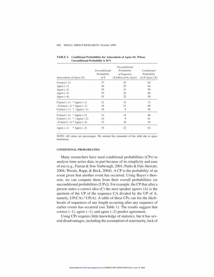
Many researchers have used conditional probabilities (CPs) toanalyze time-series data, in part because of its simplicity and easeof use (e.g., Farran & Son-Yarbrough, 2001; Parks & Fals-Stewart,2004; Woods, Rapp, & Beck, 2004). A CP is the probability of anevent given that another event has occurred. Using Bayes’s theo-rem, we can compute them from their overall probabilities (orunconditional probabilities [UPs]). For example, the CP that after aperson states a correct idea (C) the next speaker agrees (A) is thequotient of the UP of the sequence CA divided by the UP of A,namely, UP(CA) / UP(A). A table of these CPs can list the likeli-hoods of sequences of any length occurring after any sequence ofearlier events has occurred (see Table 1). The results suggest thatcorrect (–1), agree (–1), and agree (–2) predict agreement.

Using CPs requires little knowledge of statistics, but it has sev-eral disadvantages, including the assumption of stationarity, lack of


TABLE 1: Conditional Probabilities for Antecedents of Agree (0), WhoseUnconditional Probability is 56%

UnconditionalUnconditional Probability Conditional

Probability of Sequence ProbabilityAntecedents of Agree (X) of X (X followed by Agree) of (X Agree X)

Correct (–1) 37 24 65Agree (–1) 56 35 64Agree (–2) 55 33 59Agree (–3) 55 34 60Agree (–4) 55 32 59

Correct (–1) * Agree (–1) 21 15 71!Correct (–1) * Agree (–1) 34 21 60Correct (–1) * ~Agree (–1) 16 9 56

Correct (–1) * Agree (–2) 23 15 68Correct (–1) * ~Agree (–2) 14 9 61~Correct (–1) * Agree (–2) 33 18 54

Agree (–1) * Agree (–2) 35 22 63…NOTE: All values are percentages. We omitted the remainder of this table due to spacelimitations.



significance tests, discrete variable requirement, and combinatorialexplosion. Without a method to identify time periods, a researcherusing CPs assumes stationarity. As a crude test, a person using CPsmight arbitrarily create time periods and test if the CPs are similarin each time period. Without significance tests, researchers mustrely on subjective, human judgment to decide if CPs differ signif-icantly. Also, CPs cannot be computed for continuous variables.Thus, one must accept a loss of precision by dividing a continuousvariable into several ranges to create discrete variables. More vari-ables increase the precision but also increase the complexity of theresults.

Last, CP results can explode combinatorially due to continuousvariables, extra explanatory variables, testing of different samplingunits, or testing of time periods. Table 1 shows the potential com-plexity of the results. For example, a researcher must computemany CPs to determine if an explanatory variable such as correct(–1) has a substantial independent effect or whether its effect stemsfrom a correlation with another explanatory variable. Creatingmultiple discrete variables from a continuous variable exacerbatesthis problem. Last, testing for heterogeneity of sampling units ornonstationarity sharply raises the complexity of the results becausethey require replication of the full set of computations for eachsampling unit or each time period.

In short, CP might be sufficient for exploratory analysis. How-ever, its shortcomings render it inadequate for rigorous testing ofnontrivial models.

SEQUENTIAL ANALYSIS

Sequential analysis (SA; described in detail in Gottman & Roy,1990) can be viewed as an advanced version of CP, often used byresearchers in various fields (e.g., Han, 2004; Koester, 2004;Lavelli & Fogel, 2005). As with CPs, SA assumes that currentactions are probabilistically determined by recent actions. Specifi-cally, SA views sequential phenomena as a discrete Markov pro-cess that can take on any one of a finite number of predefined states.The current state determines the probability of the phenomenon




being in a given state in the next period (Papoulis, 1984). SA esti-mates the transition probabilities between the predefined states. SAalso aims to explain asymmetries in these probabilities with amodel of explanatory variables.

Unlike CP, SA includes tests of significant differences, effectsizes, and log-linear explanatory models. To test the significance ofdifferences in probabilities, SA compares how much the CP of theconsequent behavior, given the antecedant behavior, deviates fromthe simple UP of the consequent behavior by using the z score(Allison & Liker, 1982; Bakeman & Gottman, 1986). Bakemanand Quera (1995) showed that the z score is similar to an adjustedcell residual from a two-way contingency table of the relationshipbetween each behavior and its immediate antecedent. Probit orLogit betas provide an estimate of the effect size of each anteced-ent (Gottman & Roy, 1990). Last, one can test whether adding aexplanatory variable improves the fit of the model by using likeli-hood ratio chi-square tests (LR"2; Anderson & Goodman, 1957).

Consider the following application of SA to our data andhypotheses. SA proceeds through the following steps: (a) samplesize, (b) coding reliability, (c) order, (d) group heterogeneity, (e)nonstationarity, and (f) log-linear explanatory models.

Sample Size and Coding Reliability

For s states and k possible lags (or a k order Markov chain), thereare sk + 1 cells. The sample size of each subject should exceed 5 timesthe number of cells, 5 # sk + 1, and 80% of the cells should have anexpected probability greater than 5 (Bakeman & Quera, 1995;Tabachnick & Fidell, 1989). Consider the above example withthree variables (correctness, evaluation, and speaker status). Cor-rectness has two possible states, right or wrong. Evaluation has fourpossible states (agree, polite disagree, rude disagree, and ignore).Mathematics status has 33 possible states, but let us simplify theminto two states, high and low. Even with this simplification, we have2 # 4 # 2 = 16 states and four possible lags, so the sample sizeshould exceed 5,242,880 (5 # 16(4+1) = 5 # 165), far more than the3,104 data points in the above study. Thus, four possible lags are




not feasible. If the groups are heterogeneous, the suggested samplesize applies to each group. As will be shown below, the groups wereheterogeneous. The group with the fewest data had 93 data points.So we must reduce the hypotheses to the following first orderMarkov chain model with only one lag:

• Correct (–1) predicts agree (0).• Agree (–1) predicts agree (0).

This Correct/Not Correct # Agree/Not Agree model has 4 states, 16cells (42), and a suggested sample size of more than 80 (5 # 16).Still, 5 of the 20 groups did not satisfy the heuristic of 80% of thecells having expected probabilities greater than 5. So our analysesproceeded with only 15 groups (new total turns = 2,577). Cohen’s(1960) kappa showed high coding reliability for agree (k = .97, z =50.6, p < .001).

Tests of Markov Chain Order,Group Heterogeneity, and Nonstationarity

We tested if the order of the Markov chain of each subject wask using likelihood ratio chi-square tests (LR"2; Anderson &Goodman, 1957). The remaining 15 groups each showed a signifi-cant link between the current state and earlier states. This resultsuggests at least a first order (t – 1) Markov chain: mean LR"2 =40.2, degrees of freedom (df) = 9, p < .001. As shown above, thelimited sample size did not allow a second order test to be run withconfidence. (All groups failed to meet the minimum sample size of320 = 5 # 43.) Running the second order LR"2 anyway questions theassumption that a first order Markov chain could fit the data couldwell, because 7 of the 15 groups showed significant second order(t – 2) links (mean for these 7 groups: LR"2 = 191.6, df = 36, p <.001).

Next, we test for group heterogeneity and nonstationarity. Theresults also showed that the groups’data were significantly hetero-geneous for a first order Markov chain, LR"2 = 313, df= 168, p <.001. So the groups could not be pooled into one data set. When




we divided each group into two equal time periods (assuming afirst order Markov chain), 9 of the 15 groups showed significantnonstationarity. The mean for these 9 groups were as follows:LR"2 = 76.4, df = 48, p < .01. So these nine groups required divi-sion into multiple homogeneous time periods for further SA.

The SA results thus far show that the data require further divi-sion into smaller data subsets because of multiple Markov chainorders, group heterogeneity, and nonstationarity. We could com-bine data from homogeneous groups with homogeneous time peri-ods together. The resultant pools of data might be sufficiently largeto fit a second order Markov chain (or higher). However, the ninegroups with nonstationarity raise a difficult problem. SA does notprovide a means for identifying homogeneous time periods. With-out identifiable time periods, the data cannot be easily analyzed.

Explanatory Model and Results

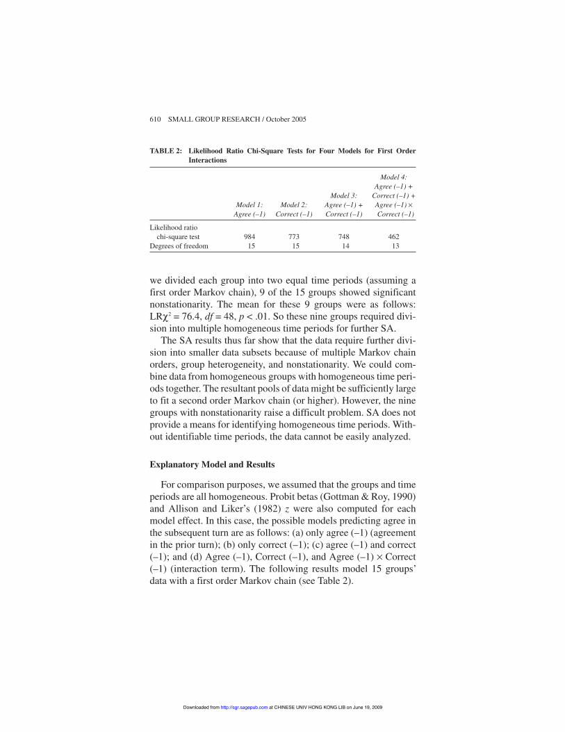
For comparison purposes, we assumed that the groups and timeperiods are all homogeneous. Probit betas (Gottman & Roy, 1990)and Allison and Liker’s (1982) z were also computed for eachmodel effect. In this case, the possible models predicting agree inthe subsequent turn are as follows: (a) only agree (–1) (agreementin the prior turn); (b) only correct (–1); (c) agree (–1) and correct(–1); and (d) Agree (–1), Correct (–1), and Agree (–1) # Correct(–1) (interaction term). The following results model 15 groups’data with a first order Markov chain (see Table 2).


TABLE 2: Likelihood Ratio Chi-Square Tests for Four Models for First OrderInteractions

Model 4:Agree (–1) +

Model 3: Correct (–1) +Model 1: Model 2: Agree (–1) + Agree (–1)

Agree (–1) Correct (–1) Correct (–1) Correct (–1)

Likelihood ratiochi-square test 984 773 748 462

Degrees of freedom 15 15 14 13



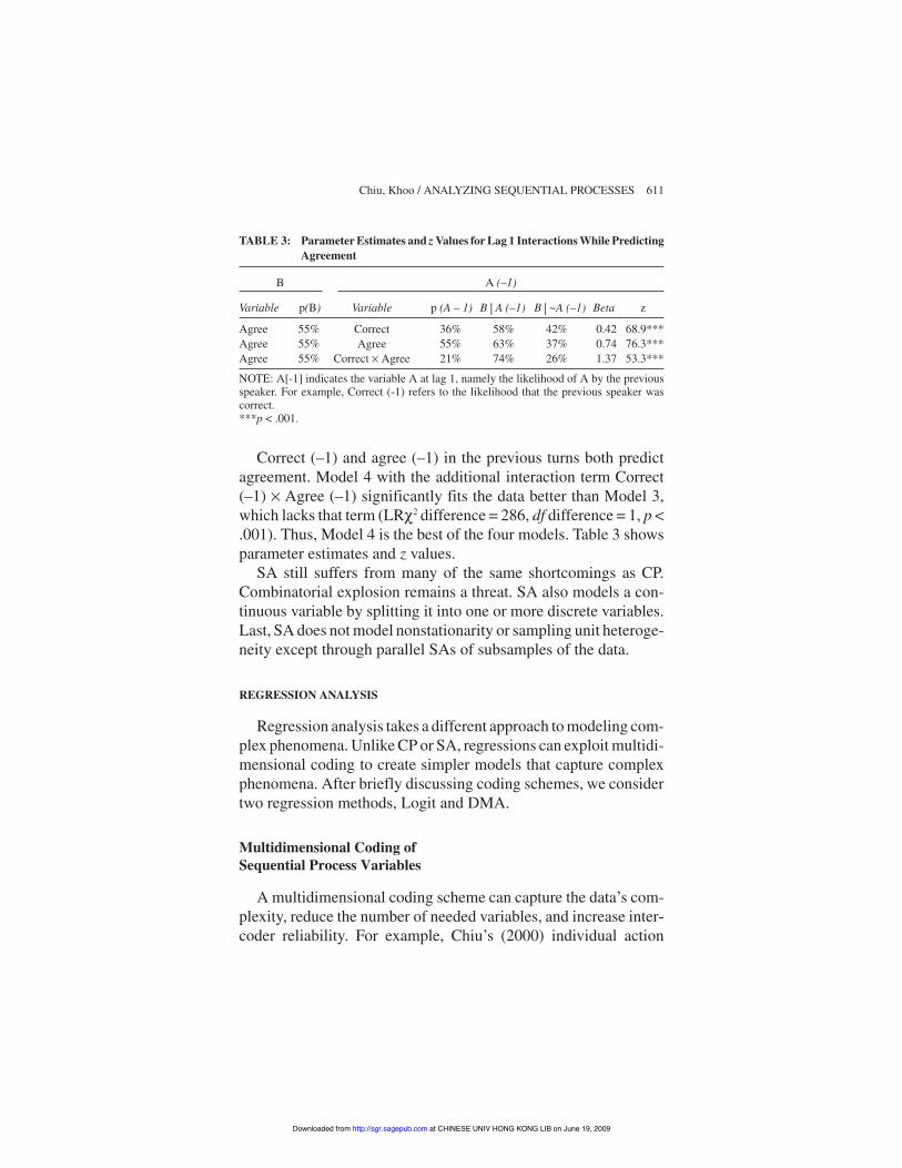
Correct (–1) and agree (–1) in the previous turns both predictagreement. Model 4 with the additional interaction term Correct(–1) # Agree (–1) significantly fits the data better than Model 3,which lacks that term (LR"2 difference = 286, df difference = 1, p <.001). Thus, Model 4 is the best of the four models. Table 3 showsparameter estimates and z values.

SA still suffers from many of the same shortcomings as CP.Combinatorial explosion remains a threat. SA also models a con-tinuous variable by splitting it into one or more discrete variables.Last, SA does not model nonstationarity or sampling unit heteroge-neity except through parallel SAs of subsamples of the data.

REGRESSION ANALYSIS

Regression analysis takes a different approach to modeling com-plex phenomena. Unlike CP or SA, regressions can exploit multidi-mensional coding to create simpler models that capture complexphenomena. After briefly discussing coding schemes, we considertwo regression methods, Logit and DMA.

Multidimensional Coding ofSequential Process Variables

A multidimensional coding scheme can capture the data’s com-plexity, reduce the number of needed variables, and increase inter-coder reliability. For example, Chiu’s (2000) individual action


TABLE 3: Parameter Estimates and z Values for Lag 1 Interactions While PredictingAgreement

B A (–1)

Variable p(B) Variable p (A – 1) B A (–1) B ~A (–1) Beta z

Agree 55% Correct 36% 58% 42% 0.42 68.9***Agree 55% Agree 55% 63% 37% 0.74 76.3***Agree 55% Correct # Agree 21% 74% 26% 1.37 53.3***

NOTE: A[-1] indicates the variable A at lag 1, namely the likelihood of A by the previousspeaker. For example, Correct (-1) refers to the likelihood that the previous speaker wascorrect.***p < .001.



framework has three dimensions. Because each dimension hasthree categories, this framework can capture 27 different types ofaction.

By coding one dimension at a time, a coder chooses among onlythree possible codes (instead of 27). Thus, training and coding timeis shorter. Intercoder reliability is also likely to improve. Further-more, by coding along different dimensions, we do not need statevariables. The smaller number of variables facilitates the use oflinear explanatory models and methods similar to ordinary leastsquares (OLS). In short, using multiple dimensions retains thecomplexity of the categories, likely improves internal consistencyand intercoder reliability, and facilitates the use of linear models.

Logit

Many sequential analyses have discrete outcome variables (e.g.,agree or not agree). When the outcome variable is discrete insteadof continuous, simple regression methods such as OLS are not suit-able, because OLS is inefficient and yields biased results.Researchers have used Logit instead to analyze time-series datawith discrete outcome variables (Gupta, 1988; Pevalin & Ermisch,2004; Silverstein & Parker, 2002). Logit is used to estimate how theprobability of observing an event (e.g., agree or not agree) is relatedto various continuous or discrete explanatory variables (for details,see Greene, 1997). In our example, the probability of current agree-ment might depend on mathematics status (–1), correct (–1), oragree (–1).

A Logit model assumes that there is a continuous, unobserved,outcome variable, y* that is linearly related to various explanatoryvariables. The unobserved variable, y*, is in turn linked to theobserved discrete outcome variable, y, by a link function. This linkfunction describes the probability that the observed outcome vari-able takes on a particular value, given the value of the unobservedvariable. A simple, often-used link function is the Logit link func-tion. To ensure that the results do not depend on the particular dis-tribution of the Logit link function, researchers often also use other




link functions with different distributions (e.g., Probit, Gompit,etc.) as tests of robustness.

Logit description. The unobserved variable in the Logit modelcan be described as

yi* = $0 + $1xi + ei (1)

To model lag effects, we can enter lag variables as explanatory vari-ables, such as correct (–1).

yi* = $0 + $1xi **Correcti – 1 + ei (2)

Let ij be the probability that an event (e.g., agreement) is observedfor at time i. It is determined by the expected value of the unob-served variable and the Logit link function:

i = p(yi = 1%xi,$0, $1 = F($0 + $1xi) (3)

=+ & +

1

1 0 1e x i( )$ $ (4)

After estimating the regression results, we facilitate their interpre-tation by converting the coefficients into percentage change in theprobability of the outcome variable. For Logit,

lnp

p1&'()

*+, = b0 + b1x1 + b2x2 + . . . + bnxn (5)

We take the antilogs and solve for p1 – p0 (p1 and p0 are the probabili-ties of the outcome variable when x1 = 1 and 0, respectively) toobtain

p pe eb b x b x b b b x b xn n n n

1 0

1

1

1

10 2 2 0 1 2 2& =

+&

++ + + + + + +( ) ( )… … (6)




Likewise for a continuous variable, the percentage change in theprobability of the outcome variable for each unit of the explanatoryvariable is

dpdx

b e

e

b b x b x b x

b b x b x b

n n

1

10 1 1 2 2

0 1 1 2 21=

+

+ + + +

+ + + +

( )

(

…

…[ ]n nx ) 2(7)

For simplicity, we discuss only binary outcome variable regres-sions. See Greene (1997) for a discussion of multinomial and or-dered outcome variables.

Applying Logit. To do an analysis, we check the sample sizerequirement, test the intercoder reliability, specify the explanatoryvariables for the Logit regression, and repeat the analyses withProbit and Gompit. The sample size requirement for regressions ismuch smaller than that for SA. Green (1991) proposed the fol-lowing heuristic sample size, N, for a multiple regression with Mexplanatory variables and an expected effect size of R2:

N > 8 (1 – R2) / R2 + M – 1

To test our hypotheses, our model requires five variables with upto four lags, or 20 (5 # 4) variables. So the model requires 811 datapoints if the expected effect size is very small; for R2 = .01 and M =20, N = 8(0.99)/0.01 + 20 – 1 = 811. Hence, the actual data set of3,104 is sufficient. (If the expected effect size is larger, the samplesize can be smaller. If the expected R2 = .05, the suggested samplesize is only 171.)

Intercoder reliability was acceptable. Evaluations included 54%agreements, 0.3% neutral, 16% ignore/unresponsive turns, 18%polite disagreements, and 9% rude disagreements (Cohen’skappa = .93, z = 49.5, p < .001).

Next, we add sets of explanatory variables to the model, priori-tized by theoretical importance and time. Correct (–1) is likely tohave the strongest effect, so we enter it first. Because the morerecent explanatory variables likely have the strongest effects, weenter the most recent remaining explanatory variables, at Lag 1,




mathematics status (–1), agree (–1), ignore (–1), and rudely dis-agree (–1). Next, we add all the explanatory variables at Lag 2, thenat Lag 3, and finally at Lag 4. Last, we test for interaction effectsamong the significant explanatory variables.

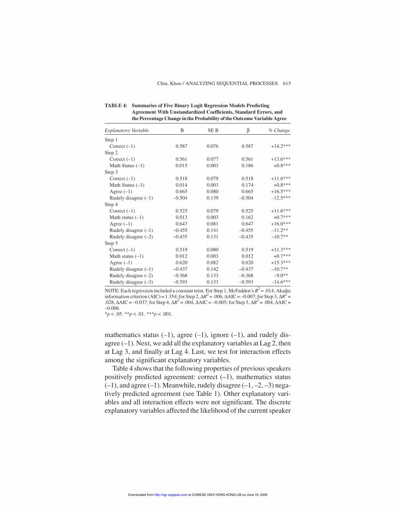
Table 4 shows that the following properties of previous speakerspositively predicted agreement: correct (–1), mathematics status(–1), and agree (–1). Meanwhile, rudely disagree (–1, –2, –3) nega-tively predicted agreement (see Table 1). Other explanatory vari-ables and all interaction effects were not significant. The discreteexplanatory variables affected the likelihood of the current speaker


TABLE 4: Summaries of Five Binary Logit Regression Models PredictingAgreement With Unstandardized Coefficients, Standard Errors, andthe Percentage Change in the Probability of the Outcome Variable Agree

Explanatory Variable B SE B % Change

Step 1Correct (–1) 0.587 0.076 0.587 +14.2***

Step 2Correct (–1) 0.561 0.077 0.561 +13.6***Math Status (–1) 0.015 0.003 0.186 +0.8***

Step 3Correct (–1) 0.518 0.079 0.518 +11.6***Math Status (–1) 0.014 0.003 0.174 +0.8***Agree (–1) 0.665 0.080 0.665 +16.5***Rudely disagree (–1) –0.504 0.139 –0.504 –12.5***

Step 4Correct (–1) 0.525 0.079 0.525 +11.6***Math status (–1) 0.013 0.003 0.162 +0.7***Agree (–1) 0.647 0.081 0.647 +16.0***Rudely disagree (–1) –0.455 0.141 –0.455 –11.2**Rudely disagree (–2) –0.435 0.131 –0.435 –10.7**

Step 5Correct (–1) 0.519 0.080 0.519 +11.3***Math status (–1) 0.012 0.003 0.012 +0.7***Agree (–1) 0.620 0.082 0.620 +15.3***Rudely disagree (–1) –0.437 0.142 –0.437 –10.7**Rudely disagree (–2) –0.368 0.133 –0.368 –9.0**Rudely disagree (–3) –0.593 0.133 –0.593 –14.6***

NOTE: Each regression included a constant term. For Step 1, McFadden’s R2 = .014, Akaikeinformation criterion (AIC) = 1.354; for Step 2, -R2 = .006, -AIC = –0.007; for Step 3, -R2 =.028, -AIC = –0.037; for Step 4, -R2 = .004, -AIC = –0.005; for Step 5, -R2 = .004, -AIC =–0.006.*p < .05. **p < .01. ***p < .001.



agreeing substantially, ranging from –14.6% (rudely disagree, –3)to +15.3% (agree, –1). Meanwhile, each 1 point increase in the pre-vious speaker’s mathematics status raised the likelihood of agree-ment by the current speaker by 0.8%.

Rudely disagree showed the strongest and longest lasting ef-fects. The coefficients for rudely disagree (–1, –2, and –3) cumula-tively exceeded correct (–1). Rudely disagree also affected the like-lihood of agree three turns later, whereas the other effects lastedonly one turn. The Probit and Gompit analyses yielded similarresults, showing that these results did not stem from the distributionassumptions (results are not shown due to space considerations;results are available from authors upon request).

Similar to SA, Logit yields estimates of effect sizes and degreeof model fit to the data. Unlike SA, Logit can test complex sets ofhypotheses with relatively small data sets, and it can model contin-uous explanatory variables. Applying Logit to subsamples of thedata serves as crude tests of nonstationarity or heterogeneity, but itdoes not model them. Logit also assumes a linear explanatorymodel and independent and identically distributed errors.

DYNAMIC MULTILEVEL ANALYSIS

Similar to Logit, DMA is based on regression analysis. It pro-ceeds through three steps: (a) identification of time periods viabreak points, (b) multilevel Logit, and (c) testing for serial correla-tion and modeling it if necessary. Although the components in thistechnique are not new, combining them in this fashion addressesshortcomings of the previous methods.

Estimating Break Points to Identify Time Periods

Suppose variable effects do not remain stable over time (non-stationary). We can model time period differences by dividing thedata into different distinct time periods and applying multilevelanalysis. First, we must identify the number and locations of breakpoints that divide a session into different time periods. Maddalaand Kim (1998) viewed the estimation of an unknown number of




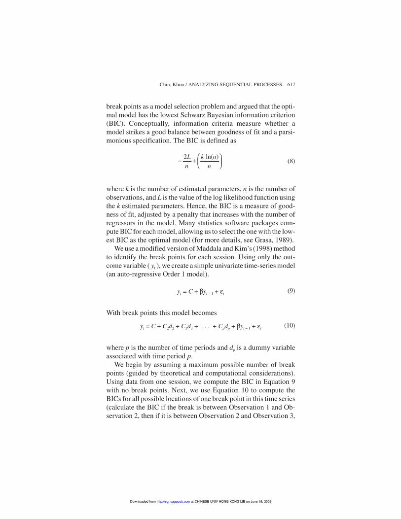
break points as a model selection problem and argued that the opti-mal model has the lowest Schwarz Bayesian information criterion(BIC). Conceptually, information criteria measure whether amodel strikes a good balance between goodness of fit and a parsi-monious specification. The BIC is defined as

& + '()

*+,

2Ln

k nn

ln( )(8)

where k is the number of estimated parameters, n is the number ofobservations, and L is the value of the log likelihood function usingthe k estimated parameters. Hence, the BIC is a measure of good-ness of fit, adjusted by a penalty that increases with the number ofregressors in the model. Many statistics software packages com-pute BIC for each model, allowing us to select the one with the low-est BIC as the optimal model (for more details, see Grasa, 1989).

We use a modified version of Maddala and Kim’s (1998) methodto identify the break points for each session. Using only the out-come variable ( yt ), we create a simple univariate time-series model(an auto-regressive Order 1 model).

yt = C + $yt – 1 + .t (9)

With break points this model becomes

yt = C + C2d2 + C3d3 + . . . + Cpdp + $yt – 1 + .t (10)

where p is the number of time periods and dp is a dummy variableassociated with time period p.

We begin by assuming a maximum possible number of breakpoints (guided by theoretical and computational considerations).Using data from one session, we compute the BIC in Equation 9with no break points. Next, we use Equation 10 to compute theBICs for all possible locations of one break point in this time series(calculate the BIC if the break is between Observation 1 and Ob-servation 2, then if it is between Observation 2 and Observation 3,




etc.) Then, we compute the BICs for all possible combinations oftwo break points, all possible combinations of three break points,and so on until we have done so for the maximum number of breakpoints.

The model with the lowest BIC has the optimal number andposition(s) of the break point(s). Repeating this procedure for eachsession identifies the number and locations of the break points in allsessions.

Researchers may have a priori information on break points. Ifthe break points are known, researchers can proceed directly to themultilevel analysis below. If they have specific candidates, they cancompare them with the break points estimated by this procedure,choose appropriate break points, and proceed with the multilevelanalysis.

Multilevel Analysis

We can model the differences across groups and across timeperiods by using multilevel analysis (Goldstein, 1995; also knownas hierarchical linear modeling, Bryk & Raudenbush, 1992). Spe-cifically, we can use it to address sampling unit–specific, session-specific, and time-period-specific effects. A multilevel model esti-mates the relationship between an outcome variable and sets ofexplanatory variables defined at different levels of analysis.

In our data, the sampling unit is the group. Each group is ob-served for only one session, so session is not a separate level ofanalysis. A speaker turn occurs within a specific time period, whichoccurs within a particular group, showing a nested hierarchicalstructure. Hence, there are three levels of analysis, speaker turn atthe lowest level, followed by time period at the next level and groupat the highest level.

A basic two-level model. The following illustrates the structureof multilevel models using a simple two-level example—speakerturns collected from different groups, with no time periods. Speakerturn variables are at Level 1. Group variables are at Level 2.




For the moment, let us use only continuous variables. Let theoutcome variable be the speaker’s fluency score for that turn (yi).Let the explanatory variable be the number of words in that turn(xi). The simple regression relationship between outcome and ex-planatory variables for each speaker turn is

yi = $0 + $1xi + ei (11)

The subscript i takes values from 1 to nj, where nj is the number ofspeaker turns in a group.

Because there are multiple groups, we allow the relationshipsto differ among the groups. We can express the multiple relation-ships as

yij = $0j + $1jxij + eij (12)

The subscript j takes a different value for each group.In multilevel analysis, the observed Level 2 groups are viewed

as a random sample of all possible groups. The parameters in eachgroup ($0j and $1j) deviate from the global parameters of all groups($0 and $1 ) by the random residuals (u0j and u1j ). So, the full multi-level model is

yij = ($0 + u0j) + ($1 + u1j)xij + eij (13)

or

yij = $0 + $1xij + u0 j+u1j x i j + e ij (14)

This equation can be divided into fixed components ($0 and $1)and random components (u0j, u1j, and eij). The random parametersall have means of zero. We assume that these random variables arenot correlated with one another and that they follow a normal distri-bution. So, it is sufficient to estimate their variances, /2

u0, /2u1, and

/2e, respectively. We can estimate the parameters of a multilevel




model (such as in the above model, $0, $1, 2u 0, /u1, and /2

e) usingmaximum likelihood methods (see Goldstein, 1995).

A three-level model for heterogeneous groups and time periods.If the data differ across groups and across time periods, we need athree-level model. The lowest level is the speaker turn. The secondlevel is the time period, and the third level is the group.

A full three-level, multilevel model with a single explanatoryvariable becomes

yijk = ($0 + u0jk + v0k) + ($1 + u1jk + v1k)xijk + eijk

or

(15)

yijk = $0 + $1xijk + u0jk + u1jkxijk + v0k + v1kxijk + eijk (16)

The subscripts, i, j, and k, refer to speaker turn i in the jth timeperiod from kth group. The subscript i takes values from 1 to njk,where njk is the number of speaker turns (Level 1) in the jth timeperiod of the kth group. The subscript j takes values from 1 to nk,where nk is the number of time periods (Level 2) in the kth group.And last, the subscript k takes a different value for each group(Level 3).

Practical considerations. Modeling data from different timeperiods, groups, and/or sessions does not always require multi-level analysis (Goldstein, 1995). The time periods, groups, or ses-sions could be homogenous. We can test for heterogeneity by run-ning a model with only a constant term and random terms for eachlevel of analysis (time period u0jkl, group v0kl, and session w0l; i.e., avariance components model):

y u v w eijkl jkl kl l ijkl= + + + +$ 0 0 0 0 (17)

If none of the random terms are statistically significant, there is noevidence for significant time period, group, or session differences.Then, a multilevel model is not needed and OLS or Logit would




suffice. If any of the random terms are significant, a multilevel anal-ysis is needed to adequately model the data.

The power issues are complicated, but the following can serve asrules of thumb (Goldstein, 1995). The sample size at the highestlevel (in this case, the group level) should be as large as possible, atleast 20. Moreover, each lower level should average at least 5 timesmore data points than the level above it (although ratios as small as3 have been successful; Chiu & Khoo, 2003). At the lowest level ofa multilevel analysis, however, the number of data points for a spe-cific group or time period can be very small, even just one (Braun,Jones, Rubin, & Thayer, 1983).

Logit and multilevel models. For discrete outcome variables, wecombine a Logit type model with multilevel analysis. The resultingmultilevel Logit models can be estimated using quasi-maximumlikelihood techniques (see Goldstein & Rasbash, 1996). Conceptu-ally, a multilevel Logit model can be divided into its multilevel partand its Logit part. Consider a basic two-level model with an unob-served variable, y ij

0 at turn i of group j, a single explanatory vari-able, xij, and a Logit link function:

y ij0 = $0 + $xij + uj + eij (18)

The probability (1ij ) that an event (e.g., agreement) occurs atturn i of group j is determined by the expected value of the unob-served variable and the Logit link function:

1ij = p(yij = 1 | xij, $0, $1 = F($0 + $1xij + µj) (19)

=+ & + +

1

1 0 1e x uij j( )$ $ (20)

The Level 2 variation parameter uj represents the deviation ofgroup j from the population norm. The Level 1 variation, eij, doesnot contribute to the fixed components and is a random variable




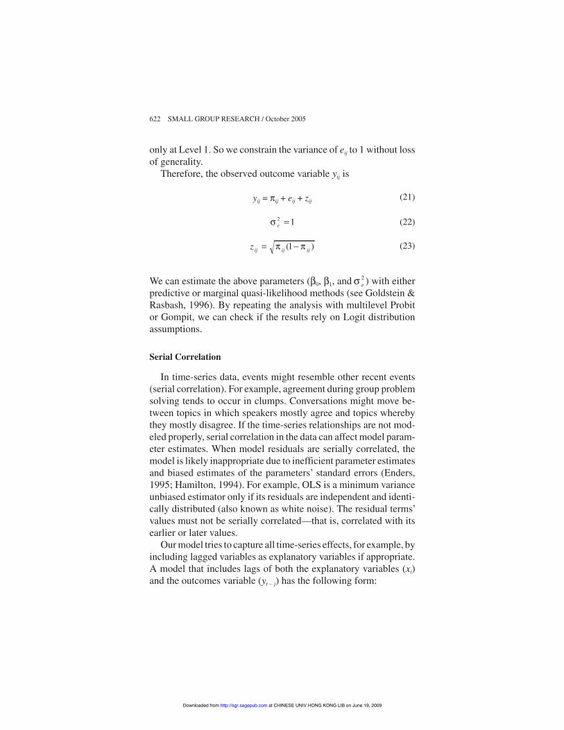
only at Level 1. So we constrain the variance of eij to 1 without lossof generality.

Therefore, the observed outcome variable yij is

yij = 1ij + eij + zij (21)

/ e2 1= (22)

z ij ij ij= &1 1( )1 (23)

We can estimate the above parameters ($0, $1, and / e2 ) with either

predictive or marginal quasi-likelihood methods (see Goldstein &Rasbash, 1996). By repeating the analysis with multilevel Probitor Gompit, we can check if the results rely on Logit distributionassumptions.

Serial Correlation

In time-series data, events might resemble other recent events(serial correlation). For example, agreement during group problemsolving tends to occur in clumps. Conversations might move be-tween topics in which speakers mostly agree and topics wherebythey mostly disagree. If the time-series relationships are not mod-eled properly, serial correlation in the data can affect model param-eter estimates. When model residuals are serially correlated, themodel is likely inappropriate due to inefficient parameter estimatesand biased estimates of the parameters’ standard errors (Enders,1995; Hamilton, 1994). For example, OLS is a minimum varianceunbiased estimator only if its residuals are independent and identi-cally distributed (also known as white noise). The residual terms’values must not be serially correlated—that is, correlated with itsearlier or later values.

Our model tries to capture all time-series effects, for example, byincluding lagged variables as explanatory variables if appropriate.A model that includes lags of both the explanatory variables (xi)and the outcomes variable (yt – j) has the following form:




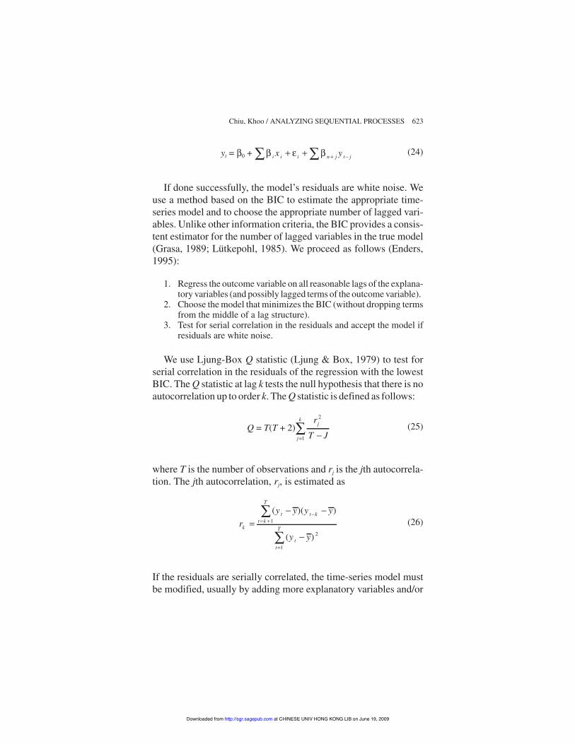
yt = $0 + $ . $i i i n j t jx y2 2+ + + & (24)

If done successfully, the model’s residuals are white noise. Weuse a method based on the BIC to estimate the appropriate time-series model and to choose the appropriate number of lagged vari-ables. Unlike other information criteria, the BIC provides a consis-tent estimator for the number of lagged variables in the true model(Grasa, 1989; Lütkepohl, 1985). We proceed as follows (Enders,1995):

1. Regress the outcome variable on all reasonable lags of the explana-tory variables (and possibly lagged terms of the outcome variable).

2. Choose the model that minimizes the BIC (without dropping termsfrom the middle of a lag structure).

3. Test for serial correlation in the residuals and accept the model ifresiduals are white noise.

We use Ljung-Box Q statistic (Ljung & Box, 1979) to test forserial correlation in the residuals of the regression with the lowestBIC. The Q statistic at lag k tests the null hypothesis that there is noautocorrelation up to order k. The Q statistic is defined as follows:

Q = T(T + 2)r

T Jj

j

k 2

1 &=2 (25)

where T is the number of observations and rj is the jth autocorrela-tion. The jth autocorrelation, rj, is estimated as

ry y y y

y yk

t t kt k

T

tt

T=

& &

&

&= +

=

2

2

( )( )

( )

1

2

1

(26)

If the residuals are serially correlated, the time-series model mustbe modified, usually by adding more explanatory variables and/or




longer lags of the explanatory variables already in the model. The Qstatistic for the final model should not reject the hypothesis thatthe residuals are not serially correlated. If the residuals are not seri-ally correlated, the time-series model is likely suitable and esti-mates are likely unbiased. This also applies to Logit and Probitmodels (Robinson, 1982).

Applying DMA

The analysis proceeded in the order described above. After com-puting the minimum sample size and intercoder reliability as withLogit, we identified the time periods and break points. Then, wetested for heterogeneity across groups and across time periods witha three-level Logit variance components model using the softwareMLn (Rasbash & Woodhouse, 1995).1 After the result showed sig-nificant variance at all three levels, we added explanatory variablesto a three-level Logit model in the same manner as the simple Logitmodel but allowing for coefficients to differ across groups andacross time periods (random effects). Third, we tested for residualserial correlation with Q statistics. If we found serial correlation,we would have modified the model to eliminate the serial correla-tion. In this specific study, there was no serial correlation in theproposed model.

As with Logit, we facilitated interpretation of the results by con-verting the coefficients into percentage of change in the probabilityof the outcome variable. To ensure that the results did not dependon the Logit distribution assumptions, the entire analysis was re-peated with multilevel Probit. (Due to space considerations, we didnot include these results, but they are available upon request.)

As noted above in the Logit regression, the sample size andintercoder reliability were adequate. The estimation of break pointsyielded one to four break points for each group, resulting in twoto five different time periods. Thus, the tendency to agree differedacross time periods within each session.

The variance components model showed significant variation ofagree at both the group level (0.14, SE = 0.05) and the time periodlevel (0.06, SE = 0.02). So the groups and the time periods were




both heterogeneous with respect to agree. Thus, a three-level multi-level model with groups, time periods, and speaker turns was suit-able. Of the total agree variance, 12% occurred at the group level,and 5% occurred at the time period level.

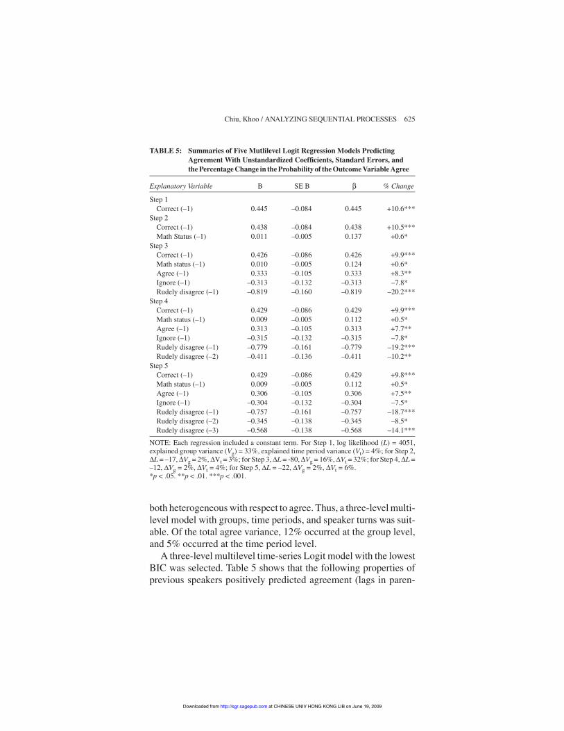
A three-level multilevel time-series Logit model with the lowestBIC was selected. Table 5 shows that the following properties ofprevious speakers positively predicted agreement (lags in paren-


TABLE 5: Summaries of Five Mutlilevel Logit Regression Models PredictingAgreement With Unstandardized Coefficients, Standard Errors, andthe Percentage Change in the Probability of the Outcome Variable Agree

Explanatory Variable B SE B % Change

Step 1Correct (–1) 0.445 –0.084 0.445 +10.6***

Step 2Correct (–1) 0.438 –0.084 0.438 +10.5***Math Status (–1) 0.011 –0.005 0.137 +0.6*

Step 3Correct (–1) 0.426 –0.086 0.426 +9.9***Math status (–1) 0.010 –0.005 0.124 +0.6*Agree (–1) 0.333 –0.105 0.333 +8.3**Ignore (–1) –0.313 –0.132 –0.313 –7.8*Rudely disagree (–1) –0.819 –0.160 –0.819 –20.2***

Step 4Correct (–1) 0.429 –0.086 0.429 +9.9***Math status (–1) 0.009 –0.005 0.112 +0.5*Agree (–1) 0.313 –0.105 0.313 +7.7**Ignore (–1) –0.315 –0.132 –0.315 –7.8*Rudely disagree (–1) –0.779 –0.161 –0.779 –19.2***Rudely disagree (–2) –0.411 –0.136 –0.411 –10.2**

Step 5Correct (–1) 0.429 –0.086 0.429 +9.8***Math status (–1) 0.009 –0.005 0.112 +0.5*Agree (–1) 0.306 –0.105 0.306 +7.5**Ignore (–1) –0.304 –0.132 –0.304 –7.5*Rudely disagree (–1) –0.757 –0.161 –0.757 –18.7***Rudely disagree (–2) –0.345 –0.138 –0.345 –8.5*Rudely disagree (–3) –0.568 –0.138 –0.568 –14.1***

NOTE: Each regression included a constant term. For Step 1, log likelihood (L) = 4051,explained group variance (Vg) = 33%, explained time period variance (Vt) = 4%; for Step 2,-L = –17, -Vg = 2%, -Vt = 3%; for Step 3, -L = -80, -Vg = 16%, -Vt = 32%; for Step 4, -L =–12, -Vg = 2%, -Vt = 4%; for Step 5, -L = –22, -Vg = 2%, -Vt = 6%.*p < .05. **p < .01. ***p < .001.



theses): correct (–1), math status (–1), and agree (–1). Meanwhile,ignore (–1) and rudely disagree (–1, –2, –3) negatively predictedagreement. All other predictors and all interaction effects were notsignificant. As with Logit, the discrete explanatory variablesaffected the likelihood of the current speaker agreeing substan-tially, ranging from –18.7% (rudely disagree, –1) to +9.8% (cor-rect, –1). Also, each 1 point increase in the previous speaker’smathematics status raised the likelihood of agreement by the cur-rent speaker by 0.5%.

Rudely disagree showed the strongest and longest lasting ef-fects. The coefficients for rudely disagree (–1 and –3) were thelargest, exceeding even correct (–1). Rudely disagree also affectedthe likelihood of agree three turns later, whereas the other effectslasted only one turn.

None of the variances of the explanatory variables’ coefficientswere significant at either the group or time period level. This resultsuggests that the explanatory variables’ effects on agreement aregeneral across both groups and time periods. After testing nestedhypotheses of successive deletions of nonsignificant explanatoryvariables (with Wald tests; see Davidson & MacKinnon, 1993), thesame significant explanatory variables remain. The Q statistics ofthe final model showed no significant serial correlation of residualsin any of the 20 groups. So the time-series model is likely appropri-ate. Repeating the analysis with multilevel Probit showed similarresults.

The results show that as expected, students are more likely toagree with a correct idea than an incorrect one. However, mathe-matical status, recent agreement, and rudeness all distorted theirevaluations of one another’s ideas. The effect of rudeness on agree-ment was larger and longer lasting than that of correctness.

COMPARISON OF THE DIFFERENT METHODS

Comparison of Results

The results from using the four methods showed some consis-tencies but several inconsistencies. They all showed that both cor-




rectness and agreement by the previous speaker raised the likeli-hood of agreement by the current speaker. Because of the sheernumber of conditional probabilities, comparing the effects of mul-tiple explanatory variables was difficult. Meanwhile, SA assump-tions were not valid for more complex models because they re-quired substantially more data. Also, the Correct (–1) # Agree (–1)interaction term was significant in SA but not in Logit or DMA.The Logit results resembled the DMA results with some excep-tions. First, Logit did not find a significant effect for ignore (–1), aresult that was evident from DMA. Also, the effect sizes differedsubstantially. For example, Logit underestimated the effects ofrudely disagree, as found in DMA.

CP, SA, and Logit do not properly test for nonstationarity. Assuggested by the results from the break point estimation, a LR"2

test on two equal time periods does not adequately test for non-stationarity. According to the SA’s LR"2 test results, only 6 of the15 groups had stationarity. However, the break point methoddivided each group into at least two different time periods, showingthat all groups had heterogeneous time periods.

Suitability of Each Method

Retaining some basic regression assumptions, DMA addressesseveral major difficulties involved in modeling the effects of recentevents on subsequent events within a series (see comparison Table6). Similar to other regressions analyses, DMA assumes a linearexplanatory model and independent and identically distributederrors. With the proper theoretical framework and coding, how-ever, DMA addresses the following difficulties: (a) the threat ofcombinatorial explosion, (b) modeling both continuous and dis-crete variables, and (c) modeling differences across time (nonsta-tionarity) and across groups (group heterogeneity).

When testing complex models, combinatorial explosion of pos-sible states threatens CP and SA but not simple regressions orDMA. As a result, SA can require prohibitively large sample sizesto yield suitable estimates of effect size and model fit. (Because CPdoes not produce these estimates, it does not require large sample




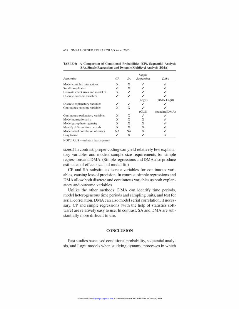
sizes.) In contrast, proper coding can yield relatively few explana-tory variables and modest sample size requirements for simpleregressions and DMA. (Simple regressions and DMA also produceestimates of effect size and model fit.)

CP and SA substitute discrete variables for continuous vari-ables, causing loss of precision. In contrast, simple regressions andDMA allow both discrete and continuous variables as both explan-atory and outcome variables.

Unlike the other methods, DMA can identify time periods,model heterogeneous time periods and sampling units, and test forserial correlation. DMA can also model serial correlation, if neces-sary. CP and simple regressions (with the help of statistics soft-ware) are relatively easy to use. In contrast, SA and DMA are sub-stantially more difficult to use.

CONCLUSION

Past studies have used conditional probability, sequential analy-sis, and Logit models when studying dynamic processes in which


TABLE 6: A Comparison of Conditional Probabilities (CP), Sequential Analysis(SA), Simple Regressions and Dynamic Multilevel Analysis (DMA)

SimpleProperties CP SA Regression DMA

Model complex interactions X X ! !Small sample size ! X ! !Estimate effect sizes and model fit X ! ! !Discrete outcome variables ! ! ! !

(Logit) (DMA-Logit)Discrete explanatory variables ! ! ! !Continuous outcome variables X X ! !

(OLS) (standard DMA)Continuous explanatory variables X X ! !Model nonstationarity X X X !Model group heterogeneity X X X !Identify different time periods X X X !Model serial correlation of errors NA NA X !Easy to use ! X ! X

NOTE: OLS = ordinary least squares.



events in a series are affected by recent past events. Coding difficul-ties and modeling of only discrete explanatory variables limit theapplicability of the conditional probability and sequential analysismethods, enabling them to model only simple phenomena. Fur-thermore, all three methods fail to address heterogeneity acrosstime or across groups.

We introduced and applied a method that addresses all of theseproblems: DMA. Given a small data set, multidimensional codingallows models with more explanatory variables, especially thosewith longer lags (from earlier turns). DMA allows both discreteand continuous variables as both outcome and explanatory vari-ables. Using break point estimation and multilevel techniques,DMA also models the heterogeneity across time periods, groups,and sessions.

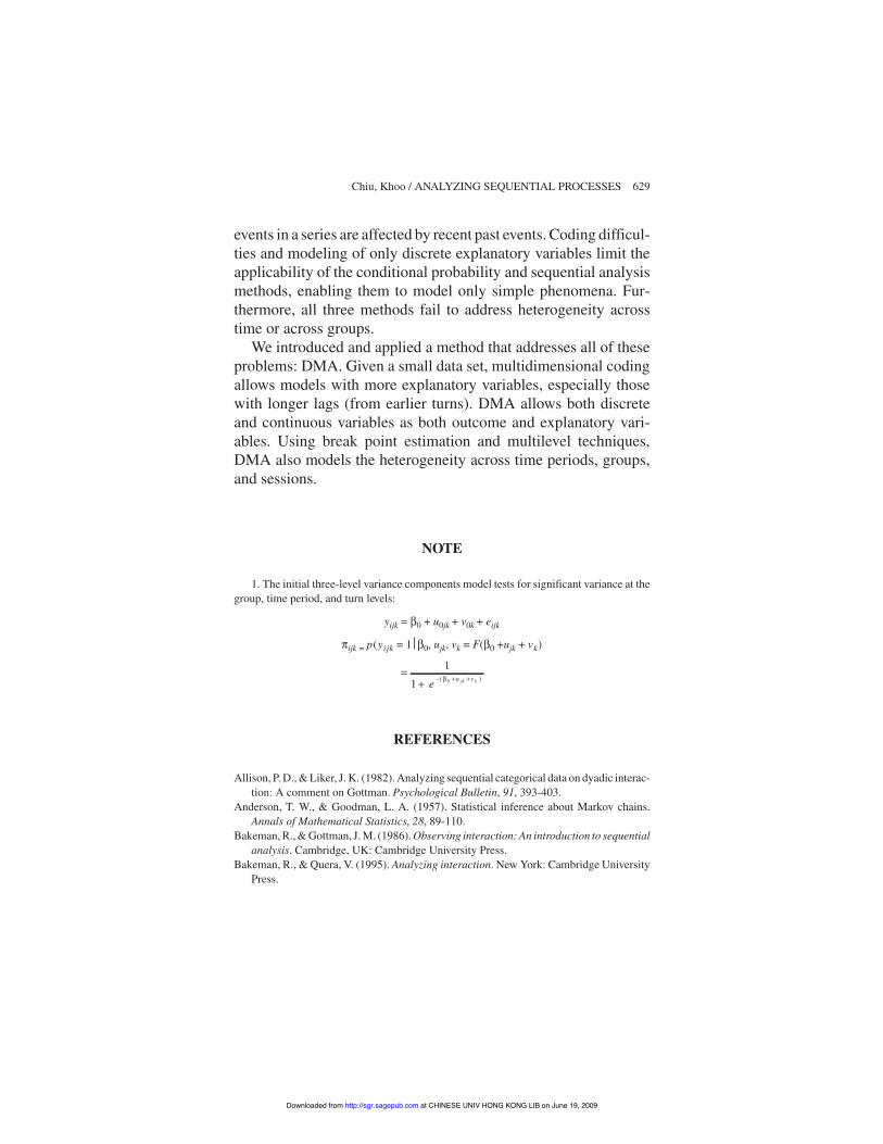
NOTE

1. The initial three-level variance components model tests for significant variance at thegroup, time period, and turn levels:

yijk = $0 + u0jk + v0k + eijk

1ijk = p(yijk = 1%$0, ujk, vk = F($0 +ujk + vk)

=+ & + +

1

1 0eu vjk k( )$

REFERENCES

Allison, P. D., & Liker, J. K. (1982). Analyzing sequential categorical data on dyadic interac-tion: A comment on Gottman. Psychological Bulletin, 91, 393-403.

Anderson, T. W., & Goodman, L. A. (1957). Statistical inference about Markov chains.Annals of Mathematical Statistics, 28, 89-110.

Bakeman, R., & Gottman, J. M. (1986). Observing interaction: An introduction to sequentialanalysis. Cambridge, UK: Cambridge University Press.

Bakeman, R., & Quera, V. (1995). Analyzing interaction. New York: Cambridge UniversityPress.




Braun, H. I., Jones, D. H., Rubin, D. B., & Thayer, D. T. (1983). Empirical Bayes estimationof coefficients in the general linear model from data of deficient rank. Psychometrika,489(2), 171-181.

Bryk, A. S., & Raudenbush, S. W. (1992). Hierarchical linear models. London: Sage.Chiu, M. M. (2000). Group problem solving processes: Social interactions and individual

actions. Journal for the Theory of Social Behavior, 30(1), 27-50.Chiu, M. M. (2004). Adapting teacher interventions to student needs during cooperative

learning: How to improve student problem solving and time-on-task. American Educa-tional Research Journal, 41, 365-399.

Chiu, M. M., & Khoo, L. (2003). Rudeness and status effects during group problem solving:Do they bias evaluations and reduce the likelihood of correct solutions? Journal of Edu-cational Psychology, 95, 506-523.

Cohen, J. (1960). A coefficient of agreement for nominal scales. Educational and Psycholog-ical Measurement, 20, 37-46.

Dabbs, J. M., Jr., & Ruback, R. B. (1987). Dimensions of group process: Amount and struc-ture of vocal interaction. In L. Berkowitz (Ed.), Advances in experimental social psychol-ogy (Vol. 20, pp. 123-169). San Diego, CA: Academic Press.

Davidson, R., & MacKinnon, J. G. (1993). Estimation and inference in econometrics.Oxford, UK: Oxford University Press.

Enders, W. (1995). Applied econometric time series. New York: John Wiley.Farran, D. C., & Son-Yarbrough, W. (2001). Title I funded preschools as a developmental

context for children’s play and verbal behaviors. Early Childhood Research Quarterly,16(2), 245-262.

Goldstein, H. (1995). Multi-level statistical models. Sydney, Australia: Edward Arnold.Goldstein, H., & Rasbash, J. (1996). Improved approximations for multi-level models with

binary responses. Journal of the Royal Statistical Society, 159, 505-13.Goodman, P. S., Ravlin, E., & Schminke, M. (1987). Understanding groups in organizations.

Research in Organizational Behavior, 9, 121-173.Gottman, J. M., Levenson, R. W., Swanson, C., Swanson, K., Tyson, R., & Yoshimoto, D.

(2003). Observing gay, lesbian and heterosexual couples’ relationships: Mathematicalmodeling of conflict interaction. Journal of Homosexuality, 45(1), 65-91.

Gottman, J. M., & Roy, A. K. (1990). Sequential analysis: A guide for behavioral research-ers. New York: Cambridge University Press.

Grasa, A. A. (1989). Econometric model selection: A new approach. Dordrecht, the Nether-lands: Kluwer.

Green, S. B. (1991). How many subjects does it take to do a regression analysis? MultivariateBehavioral Research, 26, 499-510.

Greene, W. H. (1997). Econometric analysis (3rd ed.). New York: Prentice Hall.Gupta, S. (1988). Impact of sales promotions on when, what, and how much to buy. Journal

of Marketing Research, 25(4), 342-355.Hamilton, J. D. (1994). Time series analysis. Princeton, NJ: Princeton University Press.Han, G. (2004). Analysis of change experience in group counseling. Constructivism in the

Human Sciences, 9, 77-94.Judge, G. G., Griffiths, W. E., Hill, R. C., Lutkepohl, H., & Lee, T. C. (1985). The theory and

practice of econometrics (2nd ed.). New York: John Wiley.Koester, A. J. (2004). Relational sequences in workplace genres. Journal of Pragmatics, 36,

1405-1428.




Lavelli, M., & Fogel, A. (2005). Developmental changes in the relationship between theinfant’s attention and emotion during early face-to-face communication: The 2-monthtransition. Developmental Psychology, 41, 265-280.

Ljung, G., & Box, G. (1979). On a measure of lack of fit in time series models. Biometrika,66, 265-270.

Lütkepohl, H. (1985). Comparison of criteria for estimating the order of a vector auto-regressive process. Journal of Time Series Analysis, 6, 35-52.

Maddala, G. S., & Kim, I. M. (1998). Unit roots, cointegration and structural change. NewYork: Cambridge University Press.

Papoulis, A. (1984). Brownian movement and markoff processes. In A. Papoulis (Ed.), Prob-ability, random variables, and stochastic processes (2nd ed., pp. 515-553). New York:McGraw-Hill.

Parks, K. A., & Fals-Stewart, W. (2004). The temporal relationship between collegewomen’s alcohol consumption and victimization experiences. Alcoholism: Clinical andExperimental Research, 28(4), 625-629.

Pevalin, D. J., & Ermisch, J. (2004). Cohabiting unions, repartnering and mental health. Psy-chological Medicine, 34(8), 1553-1559.

Rasbash, J., & Woodhouse, G. (1995). MLn command reference. London: Institute of Educa-tion, Multilevel Models Project.

Robinson, P. M. (1982). On the asymptotic properties of estimators with limited dependentvariables. Econometrica, 50, 27-42.

Silverstein, M., & Parker, M. G. (2002). Leisure activities and quality of life among the oldestold in Sweden. Research on Aging, 24(5), 528-547.

Tabachnick, B. G., & Fidell, L. S. (1989). Using multivariate statistics (2nd ed.). New York:Harper & Row.

Woods, D. L., Rapp, C. G., & Beck, C. (2004). Escalation/de-escalation patterns of behav-ioral symptoms of persons with dementia. Aging and Mental Health, 8(2), 126-132.

Ming Ming Chiu (Ph.D., University of California, Berkeley, 1996) is an associateprofessor of educational psychology at the Chinese University of Hong Kong. Heexamines classroom interactions and designs statistical analyses of complex data.Recently, he published several articles on students’ interactions during group prob-lem solving and on the academic achievement of 193,076students from 41 countries.

Lawrence Khoo (Ph.D., Harvard, 1996) is a lecturer of economics at City Universityof Hong Kong. He does research on statistical methods, fertility, and resource distri-bution. Recently, he examined the effects of status and politeness on group problemsolving, developed an overlapping-generations model for changes in women’s fertil-ity, and examined cross-country differences among students using large-scale inter-national studies.




A New Method for Analyzing Sequential Processes: Dynamic Multilevel Analysis

Documents