A New Mapping Algorithm for Vehicle CAN BUS Mapping ...

A New Mapping Algorithm for Vehicle CAN BUS Mapping Based on Correlation Method

by

Feng Han

A thesis submitted in partial fulfillmentof the requirements for the degree of

Master of Science(Computer and Information Science)

in the University of Michigan-Dearborn2022

Master’s Thesis Committee:

Professor Di Ma, ChairAssociate Professor Jinhua GuoAssistant Professor Zheng Song

Acknowledgements

I would like to thank those people who have provided precious assistance on my master thesis.

My deepest gratitude goes foremost to Professor Di Ma, my supervisor, who has led me through

all the processes of the writing of this thesis. Her accurate comments, constant encouragement, and

guidance have greatly encouraged me in my academic pursuit. She helped me with every detail

in my thesis content and writing. Without her consistent and illuminating instruction, this thesis

could not have reached this level.

Secondly, I would like to express my heartfelt thanks to the committee members, Professor

Jinhua Guo and Professor Zheng Song, who give me a chance to share my research about my

favorite subject: vehicle communication. And could give me priceless comments about the thesis

when pursuing the Master’s Degree in Computer and Information Science of UM-Dearborn.

I also greatly appreciate the assistance offered by our team members, Dr. Weixing Zhou, and

Dr. Linxi Zhang. Our project could be completed to this stage is the effort from everyone in this

team. Problems become easier under our joint work. Without a team like this, my thesis would not

have been finished.

Last, I am deeply indebted to my beloved parents and friends, who always supported me, will-

ingly discussed with me, and offered valuable insights. Their help and support have accompanied

me through the difficult course of the thesis and moments of my life.

ii

Table of Contents

Acknowledgements . . . . . . . . . . . . . . . . . . . . . . . . . . . . . . . . . . . . . . ii

List of Tables . . . . . . . . . . . . . . . . . . . . . . . . . . . . . . . . . . . . . . . . . vi

List of Figures . . . . . . . . . . . . . . . . . . . . . . . . . . . . . . . . . . . . . . . . vii

Abstract . . . . . . . . . . . . . . . . . . . . . . . . . . . . . . . . . . . . . . . . . . . . ix

Chapter 1 Introduction . . . . . . . . . . . . . . . . . . . . . . . . . . . . . . . . . . 1

1.1 Vehicle Network and CAN bus . . . . . . . . . . . . . . . . . . . . . . . . . . . . 1

1.2 CAN Message Mapper . . . . . . . . . . . . . . . . . . . . . . . . . . . . . . . . 2

1.2.1 Needs for a CAN Message Mapper . . . . . . . . . . . . . . . . . . . . . 2

1.2.2 CANvas Source Mapper and its Issues . . . . . . . . . . . . . . . . . . . . 4

1.2.3 Our Innovation . . . . . . . . . . . . . . . . . . . . . . . . . . . . . . . . 6

1.3 Contribution . . . . . . . . . . . . . . . . . . . . . . . . . . . . . . . . . . . . . . 7

1.4 Thesis structure . . . . . . . . . . . . . . . . . . . . . . . . . . . . . . . . . . . . 8

Chapter 2 Background . . . . . . . . . . . . . . . . . . . . . . . . . . . . . . . . . . . 9

2.1 Vehicle Network . . . . . . . . . . . . . . . . . . . . . . . . . . . . . . . . . . . 9

2.1.1 CAN Bus . . . . . . . . . . . . . . . . . . . . . . . . . . . . . . . . . . . 10

2.1.2 Other Networks . . . . . . . . . . . . . . . . . . . . . . . . . . . . . . . . 19

2.2 Security Solution . . . . . . . . . . . . . . . . . . . . . . . . . . . . . . . . . . . 20

Chapter 3 System Requirements . . . . . . . . . . . . . . . . . . . . . . . . . . . . . 23

3.1 Choose A Mapper Algorithm Type . . . . . . . . . . . . . . . . . . . . . . . . . . 23

3.2 Time complexity and Space complexity requirement . . . . . . . . . . . . . . . . 24

3.3 Mapping tool structure . . . . . . . . . . . . . . . . . . . . . . . . . . . . . . . . 25

iii

3.3.1 Data Format . . . . . . . . . . . . . . . . . . . . . . . . . . . . . . . . . 25

3.3.2 Data Extraction . . . . . . . . . . . . . . . . . . . . . . . . . . . . . . . . 26

3.3.3 Data Classification . . . . . . . . . . . . . . . . . . . . . . . . . . . . . . 29

3.3.4 Tracker . . . . . . . . . . . . . . . . . . . . . . . . . . . . . . . . . . . . 29

3.3.5 Enumeration . . . . . . . . . . . . . . . . . . . . . . . . . . . . . . . . . 30

3.3.6 End . . . . . . . . . . . . . . . . . . . . . . . . . . . . . . . . . . . . . . 30

Chapter 4 Source Mapper Design and Improvements . . . . . . . . . . . . . . . . . . 32

4.1 CANvas+ . . . . . . . . . . . . . . . . . . . . . . . . . . . . . . . . . . . . . . . 32

4.1.1 CANvas Algorithm . . . . . . . . . . . . . . . . . . . . . . . . . . . . . . 32

4.1.2 CANvas+ Algorithm . . . . . . . . . . . . . . . . . . . . . . . . . . . . . 33

4.2 Machine Learning Based Source Mapping . . . . . . . . . . . . . . . . . . . . . . 35

4.3 Covariance . . . . . . . . . . . . . . . . . . . . . . . . . . . . . . . . . . . . . . 36

4.3.1 Covariance Algorithm . . . . . . . . . . . . . . . . . . . . . . . . . . . . 36

4.3.2 Relevant Parameters Definition . . . . . . . . . . . . . . . . . . . . . . . . 38

4.3.3 Covariance Improvement . . . . . . . . . . . . . . . . . . . . . . . . . . . 42

Chapter 5 Data Collection . . . . . . . . . . . . . . . . . . . . . . . . . . . . . . . . . 48

5.1 Data Collection Tool . . . . . . . . . . . . . . . . . . . . . . . . . . . . . . . . . 48

5.1.1 ELM327 . . . . . . . . . . . . . . . . . . . . . . . . . . . . . . . . . . . 49

5.1.2 ZLG Canalyst . . . . . . . . . . . . . . . . . . . . . . . . . . . . . . . . . 50

5.1.3 Vector Canalyzer . . . . . . . . . . . . . . . . . . . . . . . . . . . . . . . 51

5.1.4 Intrepid . . . . . . . . . . . . . . . . . . . . . . . . . . . . . . . . . . . . 51

5.2 Data source . . . . . . . . . . . . . . . . . . . . . . . . . . . . . . . . . . . . . . 52

5.2.1 BUSMASTER Data . . . . . . . . . . . . . . . . . . . . . . . . . . . . . 53

5.2.2 Black Box Data . . . . . . . . . . . . . . . . . . . . . . . . . . . . . . . . 53

5.2.3 Arduino Data . . . . . . . . . . . . . . . . . . . . . . . . . . . . . . . . . 55

5.2.4 Bench Data . . . . . . . . . . . . . . . . . . . . . . . . . . . . . . . . . . 55

iv

5.2.5 Vehicle Data . . . . . . . . . . . . . . . . . . . . . . . . . . . . . . . . . 57

5.3 Summary . . . . . . . . . . . . . . . . . . . . . . . . . . . . . . . . . . . . . . . 59

Chapter 6 Vehicle Information Database . . . . . . . . . . . . . . . . . . . . . . . . . 62

6.1 Database Platform . . . . . . . . . . . . . . . . . . . . . . . . . . . . . . . . . . . 62

6.1.1 Postgre Database Platform . . . . . . . . . . . . . . . . . . . . . . . . . . 63

6.1.2 Google Cloud SQL . . . . . . . . . . . . . . . . . . . . . . . . . . . . . . 63

6.2 Database Design . . . . . . . . . . . . . . . . . . . . . . . . . . . . . . . . . . . 64

6.2.1 Requirement Analysis . . . . . . . . . . . . . . . . . . . . . . . . . . . . 64

6.2.2 Design Analysis . . . . . . . . . . . . . . . . . . . . . . . . . . . . . . . 66

6.2.3 Database Exhibition . . . . . . . . . . . . . . . . . . . . . . . . . . . . . 67

Chapter 7 Result Analysis . . . . . . . . . . . . . . . . . . . . . . . . . . . . . . . . . 68

7.1 CANvas+ Analysis . . . . . . . . . . . . . . . . . . . . . . . . . . . . . . . . . . 68

7.2 Covariance Analysis . . . . . . . . . . . . . . . . . . . . . . . . . . . . . . . . . 68

Chapter 8 Conclusion and Future Work . . . . . . . . . . . . . . . . . . . . . . . . . 74

8.1 Conclusion . . . . . . . . . . . . . . . . . . . . . . . . . . . . . . . . . . . . . . 74

8.2 Future Work . . . . . . . . . . . . . . . . . . . . . . . . . . . . . . . . . . . . . . 74

References . . . . . . . . . . . . . . . . . . . . . . . . . . . . . . . . . . . . . . . . . . 76

v

List of Tables

1.1 Summary about vehicle security situation from Kim et.al [9] . . . . . . . . . . . . 4

2.1 Different structure of in-vehicle network . . . . . . . . . . . . . . . . . . . . . . . 20

3.1 Normal boards flash memory from ST company . . . . . . . . . . . . . . . . . . . 25

3.2 Collected data format . . . . . . . . . . . . . . . . . . . . . . . . . . . . . . . . . 26

4.1 Notation Table . . . . . . . . . . . . . . . . . . . . . . . . . . . . . . . . . . . . . 39

4.2 Normalized average time value from messages generated by the same module . . . 45

5.1 4 different CAN sniffing tools comparison . . . . . . . . . . . . . . . . . . . . . . 49

5.2 CAN message builder in BUSMASTER . . . . . . . . . . . . . . . . . . . . . . . 53

5.3 Black box grouped ground truth . . . . . . . . . . . . . . . . . . . . . . . . . . . 54

5.4 Vehicles used for data collection . . . . . . . . . . . . . . . . . . . . . . . . . . . 59

5.5 Data collection summary . . . . . . . . . . . . . . . . . . . . . . . . . . . . . . . 61

7.1 Standard result for Black box emulator . . . . . . . . . . . . . . . . . . . . . . . . 69

7.2 Covariance dashboard emulator result . . . . . . . . . . . . . . . . . . . . . . . . 70

7.3 Comparison between CANvas(LCM) and Covariance on number of the ECU . . . 73

vi

List of Figures

1.1 ECU mapper schematic diagram . . . . . . . . . . . . . . . . . . . . . . . . . . . 5

2.1 Demonstration of the in-vehicle network . . . . . . . . . . . . . . . . . . . . . . . 12

2.2 The high speed CAN electric signal on bus . . . . . . . . . . . . . . . . . . . . . . 12

2.3 The low speed CAN electric signal on bus . . . . . . . . . . . . . . . . . . . . . . 13

2.4 Demonstration of CAN frame . . . . . . . . . . . . . . . . . . . . . . . . . . . . 15

2.5 Demonstration of arbitration on CAN bus . . . . . . . . . . . . . . . . . . . . . . 16

2.6 Vehicle network of a passenger vehicle . . . . . . . . . . . . . . . . . . . . . . . . 18

2.7 Security Gateway Module in vehicle network structure . . . . . . . . . . . . . . . 21

3.1 The flow chart of the mapper tool . . . . . . . . . . . . . . . . . . . . . . . . . . . 25

3.2 Sample of collected data . . . . . . . . . . . . . . . . . . . . . . . . . . . . . . . 27

3.3 Data extraction of offline data . . . . . . . . . . . . . . . . . . . . . . . . . . . . 27

3.4 Data extraction of real time data . . . . . . . . . . . . . . . . . . . . . . . . . . . 28

3.5 Calculate the data period . . . . . . . . . . . . . . . . . . . . . . . . . . . . . . . 29

3.6 Judgment of the data period . . . . . . . . . . . . . . . . . . . . . . . . . . . . . . 31

4.1 Example of the Covariance method . . . . . . . . . . . . . . . . . . . . . . . . . . 37

4.2 Covariance method group method . . . . . . . . . . . . . . . . . . . . . . . . . . 40

4.3 The flowchart of implementing the Covariance using C++ . . . . . . . . . . . . . . 41

4.4 Average time from different message IDs that are from same ECU . . . . . . . . . 44

4.5 Three conditions for the similar function hardware characteristic test . . . . . . . . 45

4.6 Initial data influence covariance value . . . . . . . . . . . . . . . . . . . . . . . . 46

5.1 ELM327 data collection tool and Android analyze software . . . . . . . . . . . . . 50

vii

5.2 Data collection process using Canalyst and user interface for the Canalyst CAN tool 50

5.3 Vector VA5610A CAN tool for Vector CANalyzer . . . . . . . . . . . . . . . . . . 51

5.4 Intrepid CAN tool for vehicle CAN data collection . . . . . . . . . . . . . . . . . 52

5.5 BUSMASTER virtual CAN bus data collection . . . . . . . . . . . . . . . . . . . 54

5.6 Black box data collection . . . . . . . . . . . . . . . . . . . . . . . . . . . . . . . 55

5.7 Bench data collecting example . . . . . . . . . . . . . . . . . . . . . . . . . . . . 56

5.8 2018 Chrysler Pacifica L under testing . . . . . . . . . . . . . . . . . . . . . . . . 57

5.9 SGW . . . . . . . . . . . . . . . . . . . . . . . . . . . . . . . . . . . . . . . . . 58

5.10 Test vehicle 2021 Dodge Durango GT . . . . . . . . . . . . . . . . . . . . . . . . 60

5.11 Test vehicle 2020 RAM 3500 Laramie Longhorn . . . . . . . . . . . . . . . . . . 61

6.1 PgAdmin4 software screenshot shows vehicle ECU data . . . . . . . . . . . . . . 63

6.2 Google Cloud . . . . . . . . . . . . . . . . . . . . . . . . . . . . . . . . . . . . . 64

6.3 E-R diagram for the vehicle information database . . . . . . . . . . . . . . . . . . 65

6.4 A sample for the ECU database table . . . . . . . . . . . . . . . . . . . . . . . . . 66

6.5 A sample for the Message database table . . . . . . . . . . . . . . . . . . . . . . . 67

6.6 A sample for the Vehicle database table . . . . . . . . . . . . . . . . . . . . . . . 67

7.1 Data processed rate for emulator data on the CANvas algorithm . . . . . . . . . . 69

7.2 Number of data grouped by CANvas algorithm and Covariance algorithm . . . . . 72

7.3 CANvas algorithm result . . . . . . . . . . . . . . . . . . . . . . . . . . . . . . . 72

7.4 Covariance algorithm result . . . . . . . . . . . . . . . . . . . . . . . . . . . . . 73

viii

Abstract

Nowadays, advanced control systems help significantly improve the performance of vehicles

from many perspectives such as safety, reliability, comfort, and so on. And those features require

sophisticated controllers known as Electronic Control Unit (ECU). ECUs will electrically guaran-

tee critical on-vehicle systems working correctly by communicating through different in-vehicle

networks. Control Area Network (CAN) is the most popular in-vehicle network. A CAN mapper,

which maps CAN messages with their corresponding source/destination ECUs, is considered as a

useful tool for in-vechicle networks to help attack detection and aftermarket vehicle improvement,

similar to Nmap for modern IP networks. The major challenge in developing such a tool is the

broadcast nature of the CAN network where CAN messages have no transmitter information by

design. Existing CAN mapper performs poorly when it is used for message source mapping over

complex CANs due to the limitation of their hardware characteristic-based algorithm. Our goal

is to develop a source mapper tool to organize CAN network messages by their control area with

improved mapping accuracy in complicated network environment. Toward this goal, we propose

Covariance, a new mapper algorithm which uses correlation information among CAN message

timestamps to map in-vehicle networks. The covariance algorithm maps messages to source ECUs

based not only on hardware characteristics but also on network function characteristics. That is

why it will work better in a more complicated network environment than the previous Canvas

source mapping algorithm which is only based hardware characteristics. We implement Covari-

ance and test it over data collected from the Arduino emulator, dashboard emulator, manufacturing

development bench, and testing vehicles by six data logging tools. Our new Covariance mapper

tool could reach an average of 77.8% accuracy based on our testing results compared with an aver-

ix

age of 51.9% of existing mappers. In addition to mapper algorithm design and development, this

thesis also contributes to the setup of ECU information database, including message information

and vehicle information affiliated, from some current Stellantis model vehicles.

x

Chapter 1

Introduction

1.1 Vehicle Network and CAN bus

Modern vehicles are becoming smart by providing driver assistant functionalities, e.g., adaptive

cruise control, line departure detection, automatic braking, automatic parking. Implementing these

functionalities requires joint computing, sensing, and controlling efforts from multiple in-vehicle

sub-systems. For example, the motion of a vehicle is controlled by all powertrain parts, including

engine, transmission, etc.

These in-vehicle sub-systems have been electrified in modern vehicles and are now controlled

by ECUs (Electrical Control Units). To complete one operation, the ECUs of different sub-systems

need to communicate a lot with each other via in-vehicle networks. For example, the transmission

ECU needs information from the engine ECU to decide the timing of changing gear, while the

engine ECU communicates with the transmission ECU to determine the gas consumption.

A modern vehicle typically has more than forty ECUs operating simultaneously, transmitting

at least 125kb of data per second [1]. The data needs to be transmitted reliably for the safety of

vehicles. Hence, a high-speed and reliable in-vehicle network is required.

CAN (Controller Area Network) bus is the state-of-the-practice standard for the in-vehicle net-

work. A CAN bus connects all ECUs in a vehicle and provides an average transmission speed

of 300 kbps to 500 kbps, which meets the speed requirement. Also, some design details of the

CAN bus communication protocol, like the message arbitration and the message validation, help

the CAN bus meets the reliability requirement.

CAN bus follows a broadcast-based communication protocol to transmit messages between

1

ECU nodes. A node broadcasts its messages on the CAN bus, and those messages are received

by multiple other nodes. A unique ID is attached to each message, to guarantee it is received by

the right receivers. The transmitted information is embedded in the data field of CAN messages.

For each CAN frame, a timestamp is attached to record the exact time the message is sent onto the

CAN bus.

1.2 CAN Message Mapper

Being able to identify the transmitting ECU and the receiving ECU for each message is im-

portant, as it provides the precondition vehicle network structure information, helps developers to

prevent the vehicle cyber-attacks, and to develop aftermarket tools. Although all messages sent

over a CAN bus can be captured, it is impossible to directly identify the sender and receivers for

each message simply by the information contained in each message (i.e., message ID, data, and

timestamp). Hence, this research aims to develop a mapper tool, similar to the Nmap[2] tool of IP

network, to identify the transmitting ECU and receiving ECUs for each CAN message.

1.2.1 Needs for a CAN Message Mapper

Cyber-attacks Detection

The rapid increase of ECU mounted on vehicles not only provides new functionalities but also

provides more attack surfaces. All modules, from the cellular network to a tiny TPM sensor [3]

which monitors the tire pressure, could be the victim and the process of vehicle hacking. Among

them, the most vulnerable parts are those modules that communicate with the external environment

outside the vehicle (e.g., WiFi, Bluetooth, and FOTA( Firmware over the air)). Attacks aiming at

those modules never stop and could cause millions of losses. Charlie Miller et al. [4] executed an

attack that can control vital functions (including throttle and brake) by injecting the virus through

the infotainment system remotely and successfully killed a 2015 Jeep Cherokee on the highway.

Moreover, they can fully control the vehicle even if the driver inside the car is trying to operate the

2

vehicle mechanically.

We observe that a typical cyber-attack on the vehicle CAN network starts from one vulnerable

ECU (which can be the infotainment unit or the TPM sensor, replacing which is accessible and

not suspicious). The attack will expand from the compromised ECU to all ECUs connected to the

CAN bus, thereby impacting more crucial functions, like brake control. To detect such attacks, a

mapper tool is needed, which can get all structures of the CAN network and track the first infected

ECU. With such a tool, the security technicians could avoid the expansion of the virus by manually

shutting off the originally infected ECU as soon as possible.

Aftermarket Tool Development

Technology companies also release software for improving existing driver assistance to achieve

autonomous driving functions. For example, Openpilot [5] can provide self-driving functionality

for Toyota or Honda vehicles. Openpilot will influence the existing in-vehicle network environ-

ment and trigger the existing intrusion detection system (IDS)[6]–[8]. To adapt to a variety of

application environments, technology companies need to know vehicle networks in-depth. There

are mapper tools available for vehicle development use: like manufactures’ .dbc files and some

manufacture developer tools, like CDA in FCA. But aftermarket tools developing companies are

not authorized to utilize those official tools. Therefore, the development of products requires an-

other solution to map out the in-vehicle network, which is a source mapper.

Also, vehicle security tool developers need the CAN mapper tool as well. Miller also did a

complete survey of how many vehicles on sale are under danger, and the result is astonishing. Ky-

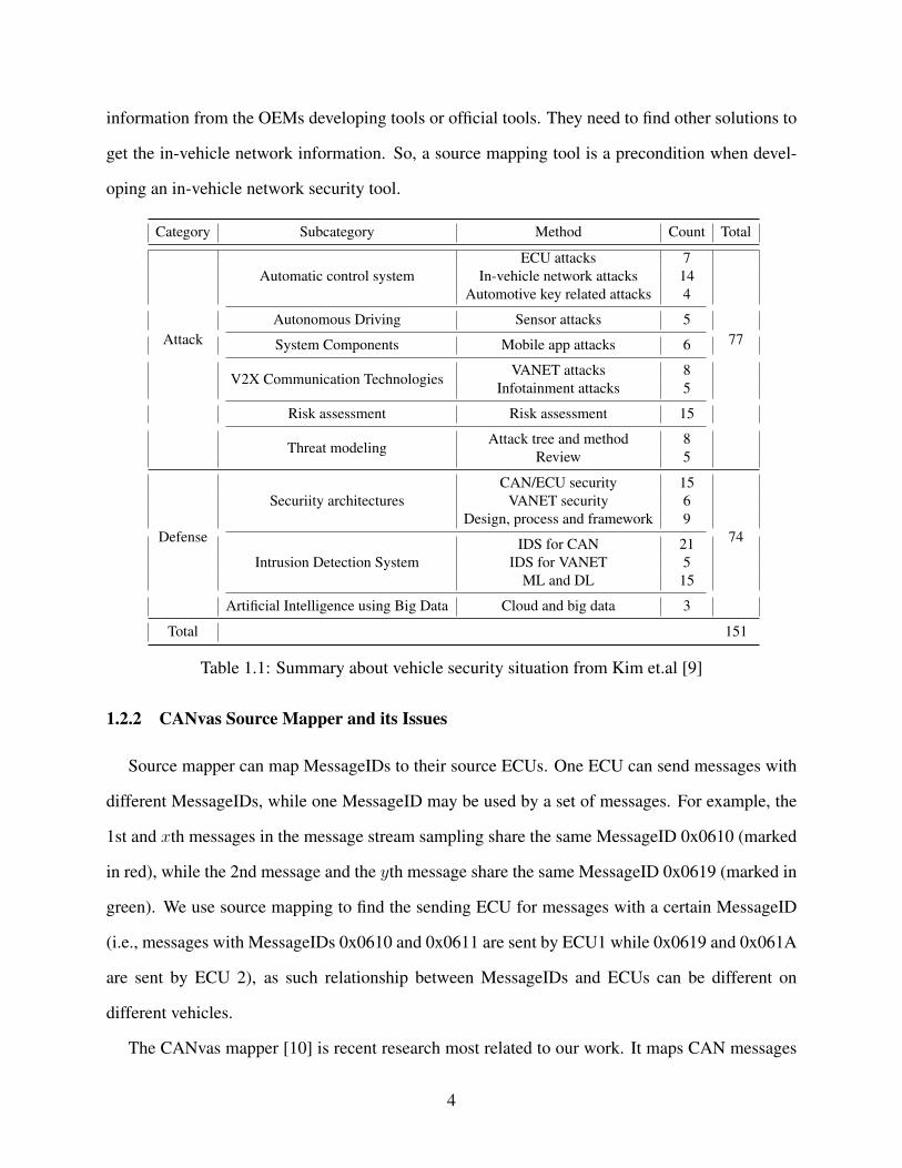
ounggon Kim et.al[9] summarizes 151 papers, as the table 1.1 shows, about cybersecurity attacks

and defenses of automotive from 2008 to 2019, and this paper includes vehicles from almost all

major vehicle brands on the US market. The security problem could happen to every vehicle, may

include the one on your driveway. Under that situation, vehicle security demands high-level secu-

rity tools. For security tool developers, they need to thoroughly understand the vehicle network

structure first. As the reason mentioned before, they hardly can gather vehicle network structure

3

information from the OEMs developing tools or official tools. They need to find other solutions to

get the in-vehicle network information. So, a source mapping tool is a precondition when devel-

oping an in-vehicle network security tool.

Category Subcategory Method Count Total

Attack

Automatic control systemECU attacks 7

77

In-vehicle network attacks 14Automotive key related attacks 4

Autonomous Driving Sensor attacks 5

System Components Mobile app attacks 6

V2X Communication TechnologiesVANET attacks 8

Infotainment attacks 5

Risk assessment Risk assessment 15

Threat modelingAttack tree and method 8

Review 5

Defense

Securiity architecturesCAN/ECU security 15

74

VANET security 6Design, process and framework 9

Intrusion Detection SystemIDS for CAN 21

IDS for VANET 5ML and DL 15

Artificial Intelligence using Big Data Cloud and big data 3

Total 151

Table 1.1: Summary about vehicle security situation from Kim et.al [9]

1.2.2 CANvas Source Mapper and its Issues

Source mapper can map MessageIDs to their source ECUs. One ECU can send messages with

different MessageIDs, while one MessageID may be used by a set of messages. For example, the

1st and xth messages in the message stream sampling share the same MessageID 0x0610 (marked

in red), while the 2nd message and the yth message share the same MessageID 0x0619 (marked in

green). We use source mapping to find the sending ECU for messages with a certain MessageID

(i.e., messages with MessageIDs 0x0610 and 0x0611 are sent by ECU1 while 0x0619 and 0x061A

are sent by ECU 2), as such relationship between MessageIDs and ECUs can be different on

different vehicles.

The CANvas mapper [10] is recent research most related to our work. It maps CAN messages

4

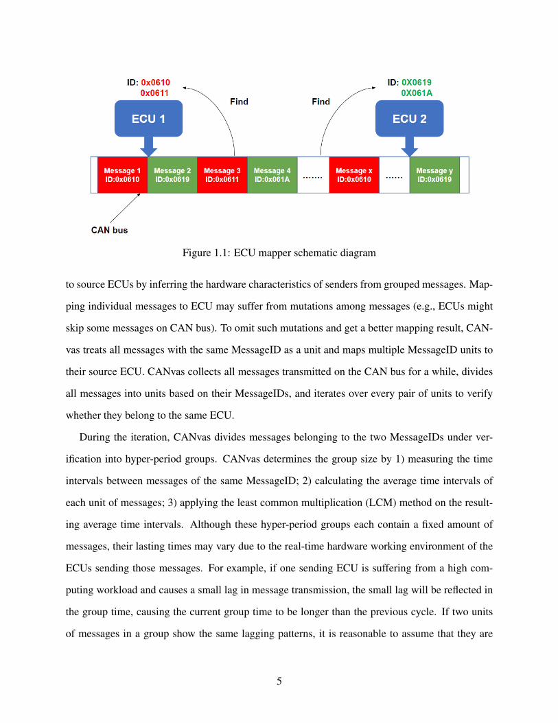
Figure 1.1: ECU mapper schematic diagram

to source ECUs by inferring the hardware characteristics of senders from grouped messages. Map-

ping individual messages to ECU may suffer from mutations among messages (e.g., ECUs might

skip some messages on CAN bus). To omit such mutations and get a better mapping result, CAN-

vas treats all messages with the same MessageID as a unit and maps multiple MessageID units to

their source ECU. CANvas collects all messages transmitted on the CAN bus for a while, divides

all messages into units based on their MessageIDs, and iterates over every pair of units to verify

whether they belong to the same ECU.

During the iteration, CANvas divides messages belonging to the two MessageIDs under ver-

ification into hyper-period groups. CANvas determines the group size by 1) measuring the time

intervals between messages of the same MessageID; 2) calculating the average time intervals of

each unit of messages; 3) applying the least common multiplication (LCM) method on the result-

ing average time intervals. Although these hyper-period groups each contain a fixed amount of

messages, their lasting times may vary due to the real-time hardware working environment of the

ECUs sending those messages. For example, if one sending ECU is suffering from a high com-

puting workload and causes a small lag in message transmission, the small lag will be reflected in

the group time, causing the current group time to be longer than the previous cycle. If two units

of messages in a group show the same lagging patterns, it is reasonable to assume that they are

5

sent by the same ECU. Therefore, CANvas observes ten hyper-periods and compares their lagging

patterns, to ascertain whether the two MessageIDs were sent by the same ECU.

The problems of the CANvas algorithm lie in its adaptability and accuracy. First, the group

size calculated by the LCM method may exceed the overall message collection time, rendering the

algorithm inapplicable. For example, for two units of messages with time intervals of 3.7s and

6.3s, the group size calculated by the LCM method is 2331s, which makes it impossible for the

CANvas algorithm to compare ten groups of messages by data collected within 20 minutes. As

a result, CANvas may fail to work stably in modern vehicle CAN systems, which feature more

ECUs and have a higher chance of generating a large LCM value.

Besides, CANvas suffers from low mapping accuracy, as it only relies on message lagging

caused by ECU hardware characteristics. Some ECU-controlled sensors can send individual mes-

sages, and these messages should be mapped to the master ECU. However, the lagging patterns

of the sensor and the ECU may be different, resulting in the sensors’ messages being incorrectly

mapped. We observe that the master ECU provides bridge connections to the sensors, rendering

their network transmission bandwidth and network latencies to be identical. The timestamps of

messages provide not only the hardware characteristics but also the network characteristics of its

sending devices, which should be fully utilized to optimize the accuracy of the mapper.

1.2.3 Our Innovation

To improve the accuracy and adaptability of the CANvas source mapper, we come up with a

novel source mapping algorithm and redesign the source mapping system. The key innovation

behind our work is that a timestamp associated with CAN messages can reveal not only the CPU’s

hardware characteristic but also its network function characteristic. We combine both character-

istics to reflect the overall ECU nodes features, then use those features to summarize the vehicle

network structure. Besides, we set a fixed value for the group time, which could help apply more

data to the algorithm.

6

1.3 Contribution

Our main contribution lies in the design and development of the Covariance source mapper

system. The system implements our new mapper algorithm, which improves the accuracy and

adaptability of the CANvas source mapper. We evaluate the effectiveness of our tool on various

testbeds, including emulators, manufacturing development bench, and testing vehicles of different

brands, and confirm that our tool achieves higher mapping accuracy than CANvas. We further

release the ground truth mapping of MessageIDs, ECUs, and vehicle models we collected from real

vehicles as an open-access database, to help other mapping algorithm researchers. In particular,

this thesis makes the following contributions:

Data Collection Methodology Study

There are multiple available sources and tools for collecting CAN messages, each featuring

unique strengths and weaknesses. Before designing our mapping system and algorithm, we first

conduct an experiential study on the data collection methodologies. In particular, we 1) build three

different kinds of testbeds (emulator, bench, and real vehicle) for data collection. The emulator is

less costly and can be used for pilot testing and parameter tuning. The bench features real sensors

and provides results similar to real cars. The real car is most costly but offers the most accurate

evaluation results; 2) compare four data collection tools popular on the market and find some tools

that may skip CAN messages which leads to lower mapping accuracy. We choose some as the

primary tools for this study as they provide the most complete results.

Design and Implement Covariance Source Mapper Tool

To map CAN bus messages to source ECUs, we build a Covariance mapper system with 2k

lines of code. The system can either capture data from the CAN bus or import data from CAN

message data files pre-captured by various third-party tools. The input data is normalized to a uni-

versal format, with various data cleaning methods filtering out unusable data. After pre-processing,

our system applies a Covariance mapping algorithm to generate the final mapping result. Our Co-

7

variance mapping algorithm utilizes the hardware and network characteristics of sending ECUs

implied in messages to improve accuracy and stability. We also make the algorithm more inclusive

and efficient by replacing the LCM-based group size with a fixed value learned from emulator data.

Evaluation

We evaluate our result based on three main testbeds: emulator, bench, and actual vehicles.

Emulator data are mainly used for tuning the group size and the Covariance parameters, while

the other two testbeds are used to verify our mapper system. The mapping ground truth data are

collected from Stellantis dbc files. To quantitatively evaluate our tool, we also implement the

CANvas mapper and conduct comparison studies on a 2021 Dodge Durango and a 2018 Chrysler

Pacifica. Our evaluation results show our system improves the mapping accuracy of CANvas from

51.9% to 77.8, thereby achieving a much better mapping result.

Open-Access Database

We release our collected ground truth data as an open-access database to benefit the research

community. Our database contains two types of data: 1) the mapping between ECUs and vehicle

models; and 2) the mapping between MessageIDs and ECUs.

1.4 Thesis structure

The rest of this thesis is arranged as follows. Chapter 2 introduces background knowledge about

CAN and other in-vehicle networks along with their security mechanisms. Chapter 3 specifies the

requirements on a mapper tool and explains how to design a source mapper system. Chapter 4

introduces our source mapper algorithms. Data collection methodology and CAN data capturing

tools comparison are discussed in chapter 5. The ground truth database is explained in chapter 6.

Chapter 7 introduces our results analysis. Last but not least, chapter 8 discusses the limitation of

our work and points out a few future directions.

8

Chapter 2

Background

The transportation ecosystem is going through a revolutionary transformation with automation

and connectivity as its main drivers. These services increase mobility and promise to virtually

eliminate crashes and fatalities which are a chronic problem to the current landscape of the au-

tomotive world. In order to deliver these promising services, automotive manufacturers have to

first eliminate malicious actors in such ecosystem and minimize their impact. The automotive

cybsersecurity is a significant problem in today’s industry. Securing vehicles includes securing in-

vehicle networks which connect various Electric Control Units (ECU) for different subsystems in

the vehicle. One of such networks is the Controller Area Network (CAN). CAN is one of the most

predominant in-vehicle bus communication protocols. This protocol was designed from Bosch in

1985 with goals of efficiency and reliability, but security was not its primary objective. [11]

2.1 Vehicle Network

Nowadays, vehicle functionalities, such as adaptive cruise control systems and lane-keep sys-

tems, will depend more on the safety, reliability, and security function [12]. Fatal accidents might

result from those malfunction from those advanced electrical systems. Moreover, the discussion

between the safety of the autonomous driving vehicle and the manually driving vehicle never

stopped. [13]–[15] Multiple reasons could cause those autonomous technologies accidents that

happened on the road. Except for the "human error," caused by the intervention of driving assist

advanced system, that often set to be the first place of the reason, "designer error" is also one of

the critical factors.[16] One profound reason beyond the "designer error" that caused those severe

9

accidents is the miscommunication between the electric control units in the vehicle network. So

vehicles need a reliable, fast, and cheap way to take the responsibility of communication in vehicles

- CAN bus.

2.1.1 CAN Bus

Control Area Network

CAN (Control Area Network) messages communication and distributed real-time control, mak-

ing it the most widely used in-vehicle network structure. CAN bus is a typical message-based pro-

tocol, so the count number of electrical modules or the priority of the electrical modules is not an

essential part of the bus network. CAN bus, as the name shows, follows the rule of the bus network,

which nodes connect directly to a common half-duplex link. [17] The host of the bus network is

called station, but no station exists in a vehicle network. So the CAN bus we currently used in the

vehicle network is a no-host version of the bus, and all the modules connected inside the network

are nodes. For all the nodes’ content networks, the CAN bus mainly follows ISO 11898-2 and ISO

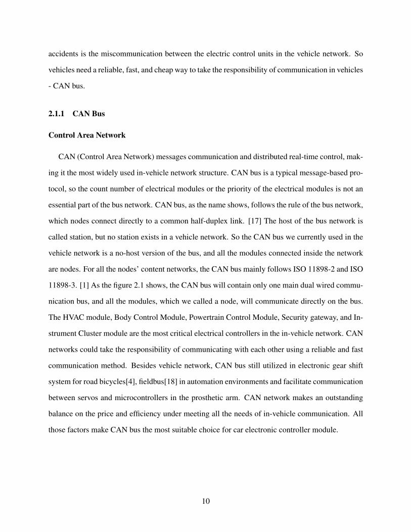
11898-3. [1] As the figure 2.1 shows, the CAN bus will contain only one main dual wired commu-

nication bus, and all the modules, which we called a node, will communicate directly on the bus.

The HVAC module, Body Control Module, Powertrain Control Module, Security gateway, and In-

strument Cluster module are the most critical electrical controllers in the in-vehicle network. CAN

networks could take the responsibility of communicating with each other using a reliable and fast

communication method. Besides vehicle network, CAN bus still utilized in electronic gear shift

system for road bicycles[4], fieldbus[18] in automation environments and facilitate communication

between servos and microcontrollers in the prosthetic arm. CAN network makes an outstanding

balance on the price and efficiency under meeting all the needs of in-vehicle communication. All

those factors make CAN bus the most suitable choice for car electronic controller module.

10

CAN principle

CAN is working based on the voltage difference between two CAN lines to guarantee the cor-

rectness of those transmitted messages. When CAN messages depart from one node, they have hex

format and could be converted directly to a digital signal. Every node on the CAN bus has a Tx

port and an Rx port. After messages going out from the node, the CAN transceiver mounted on the

controller module will help the digital signal sent from the node converted to the CAN bus format

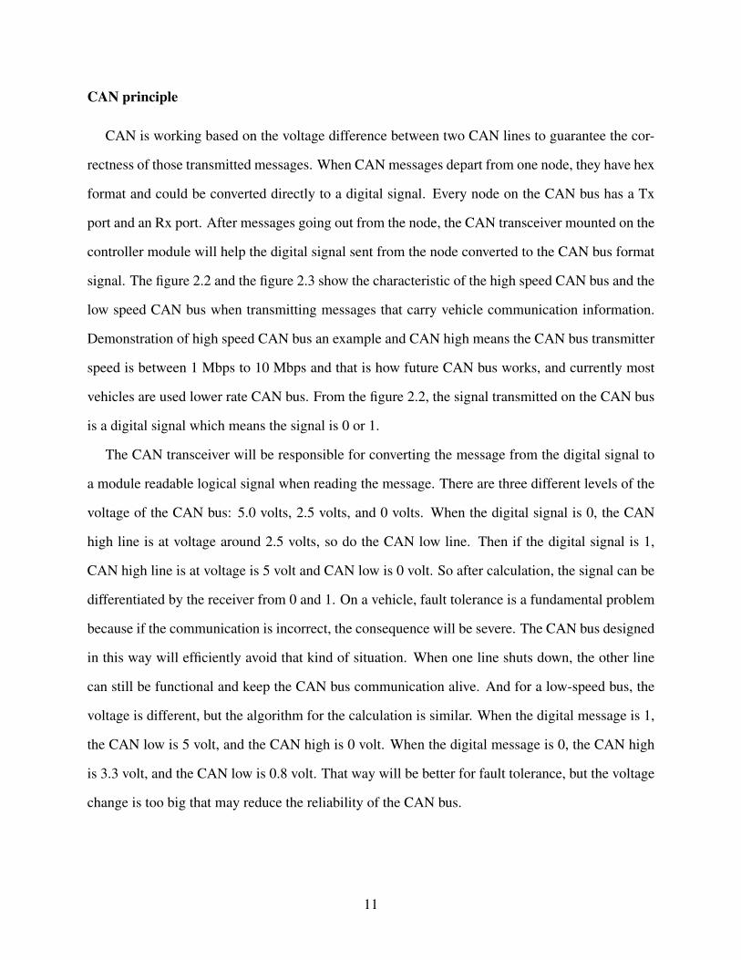
signal. The figure 2.2 and the figure 2.3 show the characteristic of the high speed CAN bus and the

low speed CAN bus when transmitting messages that carry vehicle communication information.

Demonstration of high speed CAN bus an example and CAN high means the CAN bus transmitter

speed is between 1 Mbps to 10 Mbps and that is how future CAN bus works, and currently most

vehicles are used lower rate CAN bus. From the figure 2.2, the signal transmitted on the CAN bus

is a digital signal which means the signal is 0 or 1.

The CAN transceiver will be responsible for converting the message from the digital signal to

a module readable logical signal when reading the message. There are three different levels of the

voltage of the CAN bus: 5.0 volts, 2.5 volts, and 0 volts. When the digital signal is 0, the CAN

high line is at voltage around 2.5 volts, so do the CAN low line. Then if the digital signal is 1,

CAN high line is at voltage is 5 volt and CAN low is 0 volt. So after calculation, the signal can be

differentiated by the receiver from 0 and 1. On a vehicle, fault tolerance is a fundamental problem

because if the communication is incorrect, the consequence will be severe. The CAN bus designed

in this way will efficiently avoid that kind of situation. When one line shuts down, the other line

can still be functional and keep the CAN bus communication alive. And for a low-speed bus, the

voltage is different, but the algorithm for the calculation is similar. When the digital message is 1,

the CAN low is 5 volt, and the CAN high is 0 volt. When the digital message is 0, the CAN high

is 3.3 volt, and the CAN low is 0.8 volt. That way will be better for fault tolerance, but the voltage

change is too big that may reduce the reliability of the CAN bus.

11

Figure 2.1: Demonstration of the in-vehicle network

Figure 2.2: The high speed CAN electric signal on bus

CAN frame format

Vehicles normally are using two different kinds of CAN buses for communication: high-speed

buses and low-speed buses. And on both buses, messages transmitted must follow the principle

of CAN frame [19] to connect on the vehicle network properly. CAN messages transferred in the

vehicle are manifested by a particular type of data frame for 11-bits CAN bus as shown in figure

2.4. The format of the CAN frame contains start-of-frame (SOF), remote transfer request (RTR),

ID, reserved block, data, CRC, data length code (DLC), acknowledgment (ACK) slot, and the end-

of-frame (EOF). Note that the time stamp parameter is not in the CAN data frame, which requires

a specific tool to collect the time information outside the frame.

12

Figure 2.3: The low speed CAN electric signal on bus

Start-of-frame(SOF) denotes the beginning of the transmission session. When other ECUs

detect a specific order of the SOF bits, ECUs will turn on the listen to function to read the rest of

the data. A remote transfer request (RTR) is for checking whether the data frame is a remote data

frame or not. No data lot is defined in a remote frame, which means it carries no data from the

vehicle network, and that kind of frame does not affect the overall information gathering. So, in

this thesis, no remote frame is under consideration for applying the mapping algorithm. ID is one

of the most critical parts of a single CAN frame. After all the ECUs recognize SOF lot, they need

to acknowledge that a specific CAN message under demand by identifying the frame’s ID part.

ECU will switch to "on" mode and obtain the information from the message frame if the message

ID matches the built inside the database. Reserved block is mainly for the personalized setup for

different manufactures. Data length code (DLC) informs the data length in advance and advises the

ECU about the data length. Then data block contains the information the message carries. For 11-

bits CAN frame, data length should be 2 to 8 bytes, and the data length is fixed and predefined in the

database for traditional CAN bus like high speed CAN and low speed CAN. But unchangeable data

length will limit the CAN performance and CAN communication channel. CAN-FD is invented

to solve this problem by flexing the data length. At the same time, the CAN channel could be

expanded and allow the data to transmit much faster. Cyclic redundancy check (CRC) is to detect

the error inside the CAN frame. Network error may change data, so the process of ensuring all the

data are correct in the frame is indispensable. End of frame is to inform the ECU this CAN frame

is over, and the ECU goes back to the waiting status. The process of transmitting CAN messages

13

is cyclic, and the quality of the ECU connection depends on the messages communicating via the

vehicle CAN network. So, the standard of CAN bus must adhere to every single CAN message

and ECU, or the message will not be recognized.

CAN characteristic

All CAN bus messages are cyclic when first designed. However, sometimes some modules

may not be activated, and no message being sent by that module. At that time, the message will

disappear from the CAN bus and may not look cyclic. But if we keep the module working all

the time, messages will be transmitted on the CAN bus with a briefly same time gap. There are

several kinds of different messages transporting on the CAN bus. They share the same bus without

affecting each other except when messages flood and require arbitration. Since we aim to design

an ECU mapping tool by the source of ECU, differentiation between message sources could be

demonstrated first. Source messages could be divided into four kinds based on the type of trans-

mitter: module source, sensor source, external tool source, and gateway source for some models.

Module source messages are mainly some control messages and communication messages. Their

aim is primarily to keep everything runs well. For example, network management messages are

to tell the central controller this module is alive. Also, messages of that kind should communicate

between different modules to send commands and feedback about the current condition of com-

pleting the command. Those messages contained network management messages, vehicle speed

messages on low-speed buses, engine information messages on low-speed bus and so on. Sensor

source messages are sent by the sensors all over the vehicle that collects data from each part under

monitoring. Those messages carry information about the operational status of the core parts of

a car, and some sensors may only send one message onto the CAN bus. Sensor-based messages

include MAF (mass airflow) message, and tire pressure sensor message, etc.

Another characteristic of CAN messages transmitted on the CAN bus is same ID message will

only have one single transmitter. But this message, at the same time, may have multiple receivers

for different kinds of utilization. For example, the vehicle speed message sent by the ESP module

14

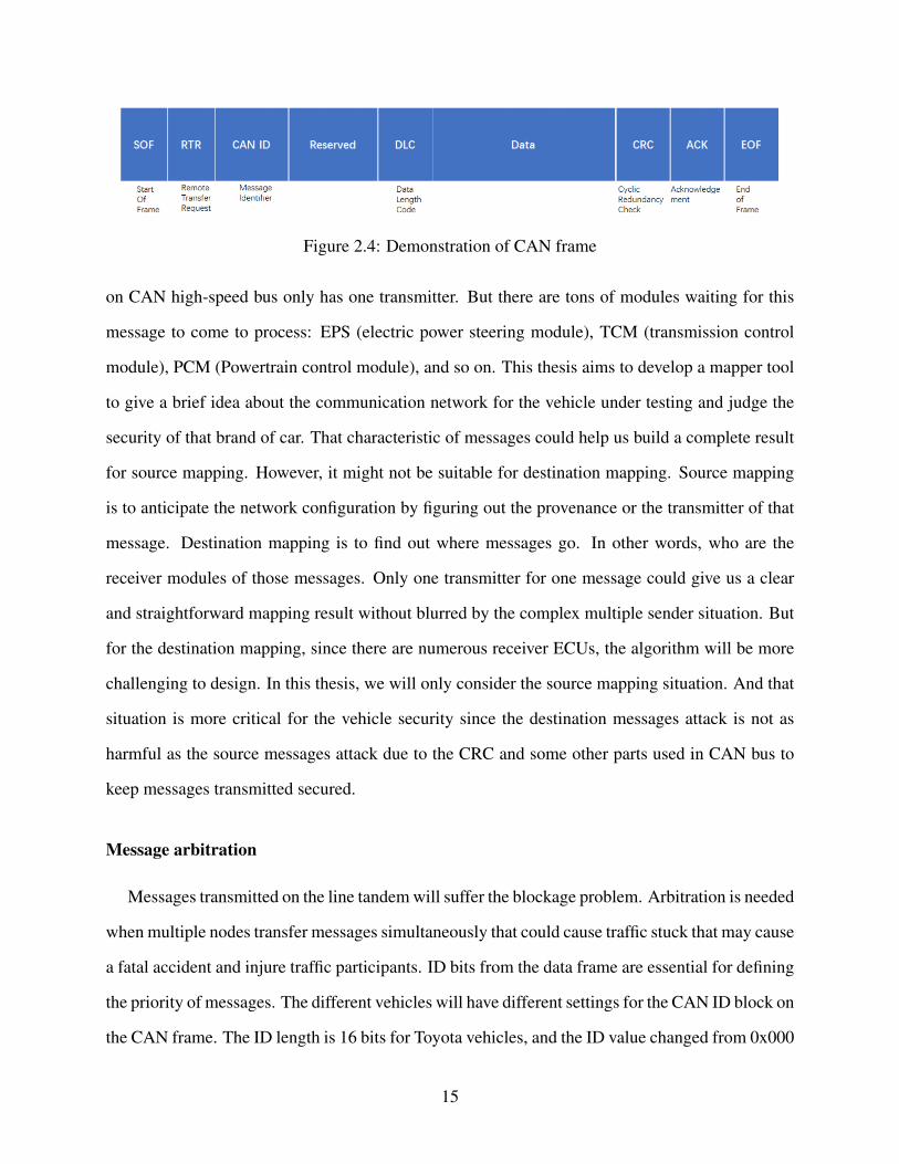
Figure 2.4: Demonstration of CAN frame

on CAN high-speed bus only has one transmitter. But there are tons of modules waiting for this

message to come to process: EPS (electric power steering module), TCM (transmission control

module), PCM (Powertrain control module), and so on. This thesis aims to develop a mapper tool

to give a brief idea about the communication network for the vehicle under testing and judge the

security of that brand of car. That characteristic of messages could help us build a complete result

for source mapping. However, it might not be suitable for destination mapping. Source mapping

is to anticipate the network configuration by figuring out the provenance or the transmitter of that

message. Destination mapping is to find out where messages go. In other words, who are the

receiver modules of those messages. Only one transmitter for one message could give us a clear

and straightforward mapping result without blurred by the complex multiple sender situation. But

for the destination mapping, since there are numerous receiver ECUs, the algorithm will be more

challenging to design. In this thesis, we will only consider the source mapping situation. And that

situation is more critical for the vehicle security since the destination messages attack is not as

harmful as the source messages attack due to the CRC and some other parts used in CAN bus to

keep messages transmitted secured.

Message arbitration

Messages transmitted on the line tandem will suffer the blockage problem. Arbitration is needed

when multiple nodes transfer messages simultaneously that could cause traffic stuck that may cause

a fatal accident and injure traffic participants. ID bits from the data frame are essential for defining

the priority of messages. The different vehicles will have different settings for the CAN ID block on

the CAN frame. The ID length is 16 bits for Toyota vehicles, and the ID value changed from 0x000

15

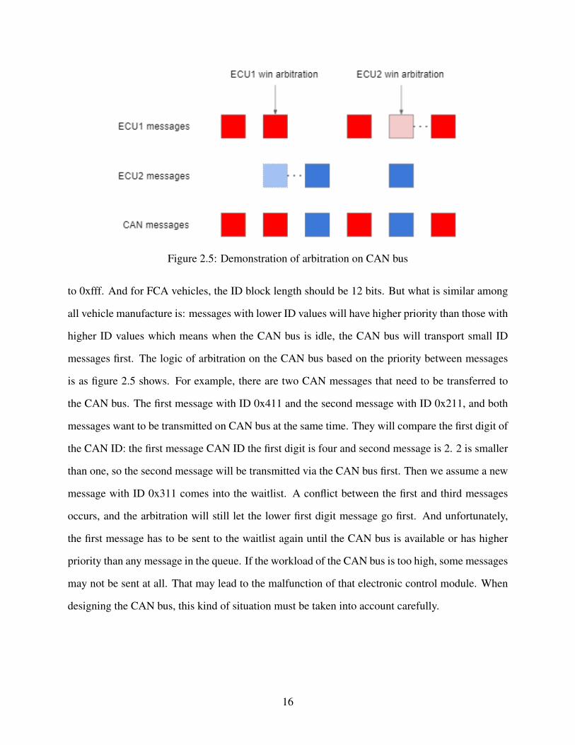
Figure 2.5: Demonstration of arbitration on CAN bus

to 0xfff. And for FCA vehicles, the ID block length should be 12 bits. But what is similar among

all vehicle manufacture is: messages with lower ID values will have higher priority than those with

higher ID values which means when the CAN bus is idle, the CAN bus will transport small ID

messages first. The logic of arbitration on the CAN bus based on the priority between messages

is as figure 2.5 shows. For example, there are two CAN messages that need to be transferred to

the CAN bus. The first message with ID 0x411 and the second message with ID 0x211, and both

messages want to be transmitted on CAN bus at the same time. They will compare the first digit of

the CAN ID: the first message CAN ID the first digit is four and second message is 2. 2 is smaller

than one, so the second message will be transmitted via the CAN bus first. Then we assume a new

message with ID 0x311 comes into the waitlist. A conflict between the first and third messages

occurs, and the arbitration will still let the lower first digit message go first. And unfortunately,

the first message has to be sent to the waitlist again until the CAN bus is available or has higher

priority than any message in the queue. If the workload of the CAN bus is too high, some messages

may not be sent at all. That may lead to the malfunction of that electronic control module. When

designing the CAN bus, this kind of situation must be taken into account carefully.

16

Modern design

CAN bus is required in all vehicles because all vehicles built since 1996 have OBD-II (On

Board Diagnostic) system to diagnose the electric failure and pass the emission control test under

the transportation process in EMIS (Environmental Management Information System) [20]. And

the OBD-II port allows the vehicle to connect with the diagnostic tools to sniff messages from the

CAN bus on a car. And for most vehicle manufacture, allow the diagnostic tools to rewrite the

module through the OBD-II port. And vehicles without OBD-II ports will not be road legal since

those vehicles cannot pass the emission test. OBD-II port built based on CAN communication

which means CAN network on every single vehicle built after 1996 are compulsory. Typically

when designing a vehicle network, there are two kinds of messages transmitted on the CAN bus.

As the figure 2.6 shows, two kinds of CAN bus( black line and red line) are designed in this

passenger car. The difference between those two kinds of the CAN bus is the transmission speed:

one is a relatively high speed, the other is relatively low speed. Different manufactures name the

CAN high-speed bus and CAN low speed bus differently. For example, Stellantis called high-

speed bus from their vehicle CAN-C and low-speed bus CAN-I. And for a newer platform for their

vehicles, they named high-speed bus CAN-FD and low-speed bus CAN-BH.

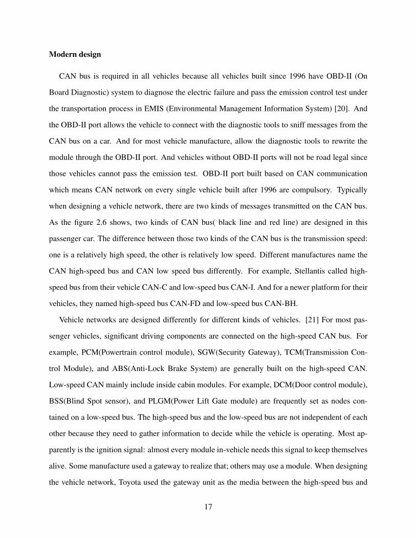
Vehicle networks are designed differently for different kinds of vehicles. [21] For most pas-

senger vehicles, significant driving components are connected on the high-speed CAN bus. For

example, PCM(Powertrain control module), SGW(Security Gateway), TCM(Transmission Con-

trol Module), and ABS(Anti-Lock Brake System) are generally built on the high-speed CAN.

Low-speed CAN mainly include inside cabin modules. For example, DCM(Door control module),

BSS(Blind Spot sensor), and PLGM(Power Lift Gate module) are frequently set as nodes con-

tained on a low-speed bus. The high-speed bus and the low-speed bus are not independent of each

other because they need to gather information to decide while the vehicle is operating. Most ap-

parently is the ignition signal: almost every module in-vehicle needs this signal to keep themselves

alive. Some manufacture used a gateway to realize that; others may use a module. When designing

the vehicle network, Toyota used the gateway unit as the media between the high-speed bus and

17

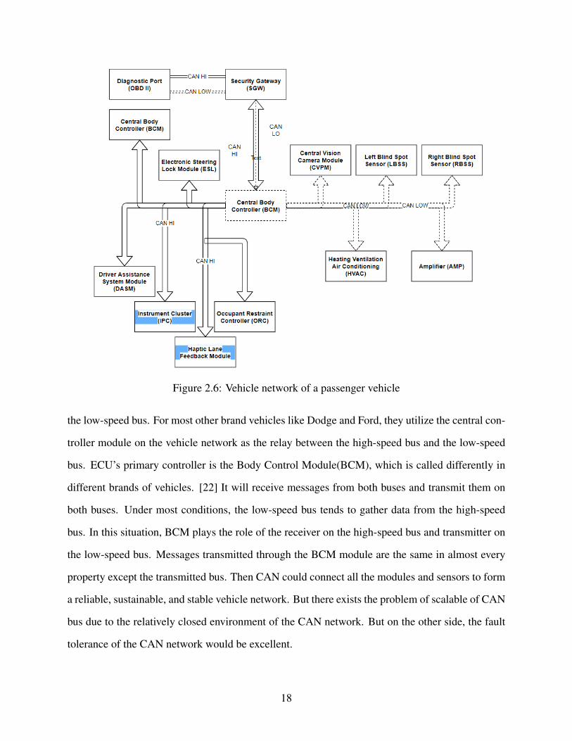
Figure 2.6: Vehicle network of a passenger vehicle

the low-speed bus. For most other brand vehicles like Dodge and Ford, they utilize the central con-

troller module on the vehicle network as the relay between the high-speed bus and the low-speed

bus. ECU’s primary controller is the Body Control Module(BCM), which is called differently in

different brands of vehicles. [22] It will receive messages from both buses and transmit them on

both buses. Under most conditions, the low-speed bus tends to gather data from the high-speed

bus. In this situation, BCM plays the role of the receiver on the high-speed bus and transmitter on

the low-speed bus. Messages transmitted through the BCM module are the same in almost every

property except the transmitted bus. Then CAN could connect all the modules and sensors to form

a reliable, sustainable, and stable vehicle network. But there exists the problem of scalable of CAN

bus due to the relatively closed environment of the CAN network. But on the other side, the fault

tolerance of the CAN network would be excellent.

18

2.1.2 Other Networks

CAN bus set to be the primary communication method for nearly 30 years. As the vehicle be-

ing developed more complex, the communication speed between controllers demands to be rapidly

increased. The traditional CAN bus is not enough to support the explode messages under trans-

mitting. Such as the 2015 RAM 1500, the truck that suffered from the stuck of the communication

traffic on CAN bus due to the limitation of traditional CAN lack communication speed. There are

several new ways to release the pressure of communication: FlexRay, CANFD, and Ethernet [23].

And the 2.1 could tell the advantages and disadvantages of each network type. Mapper algorithms

only include the CAN bus communication method in this thesis.

FlexRay

FlexRay[24] and CANFD[25] are two similar method. Both systems are built based on CAN

bus but have an extended function that can make the data length flexible. In the traditional CAN

bus, all the messages’ data lengths are fixed, and no action could change the rate unless flashing

the module with updated software. But in FlexRay and CANFD allow the same message to send

multiple different lengths of messages. That will make the vehicle network utilized more efficiently

and enormously promote the speed of CAN buses. FlexRay and CANFD could easily support 10

Mbps or more under multiple transmission aisles on the vehicle network. But the disadvantage is

that the price of construct a FlexRay network is compared with the CAN bus is much higher. So,

those two methods are mainly loaded on the high-end trim of the one auto brand.

Ethernet

Ethernet is a customarily used Internet connection method and one of the communication meth-

ods in vehicle networks.[26] That is a new challenge for the automaker as the fault tolerance of

Ethernet is the worst among all the communication methods. But on the vehicle, fault tolerance

is of vital importance because that will directly connect to the safety of traffic participants. So

Ethernet, for now mainly used for the telematic module on vehicles that its primary function is

19

Network Type Construct Cost Fault ToleranceCAN Medium High

FlexRay & CANFD High MediumEthernet Low Low

Table 2.1: Different structure of in-vehicle network

to exchange data from the client vehicle and cloud database. Meanwhile, in this thesis, we did

not contain those technologies in-vehicle network. We only consider traditional CAN bus condi-

tions, and in the future, we will add more information about this new technology since the internal

principle is similar.

LIN

Also, the LIN bus is a kind of vehicular network in modern vehicles.[27] LIN bus is mainly for

extremely low-speed bus use, and that bus is not connectable from outside the vehicle network.

This bus is primarily for the relatively independent module in the vehicle, like the door panel

module and switch. Since the LIN bus is not communicating with other modules in the car, we can

hardly get any information from the LIN bus. And the baud rate of the LIN bus is as low as 20

Kbps, so the algorithm design based on the LIN bus may not be referential. And we skipped the

LIN bus on the vehicle in this thesis.

2.2 Security Solution

Manufacture security solution

To solve the vulnerabilities mentioned above, different vehicle manufacturers provide various

solutions to them. One trending solution for that is to add a module that works as a filter to clean out

unrecognized messages that try to inject into the CAN bus. The gateway module will be set close

to the center module of the vehicle, like BCM or Gateway module, to filter out malicious messages

at the controller spec [28]. From figure 2.7 we can conclude that the security gateway module is

designed to prevent any unauthorized messages go into the CAN network in advance. For Stellan-

20

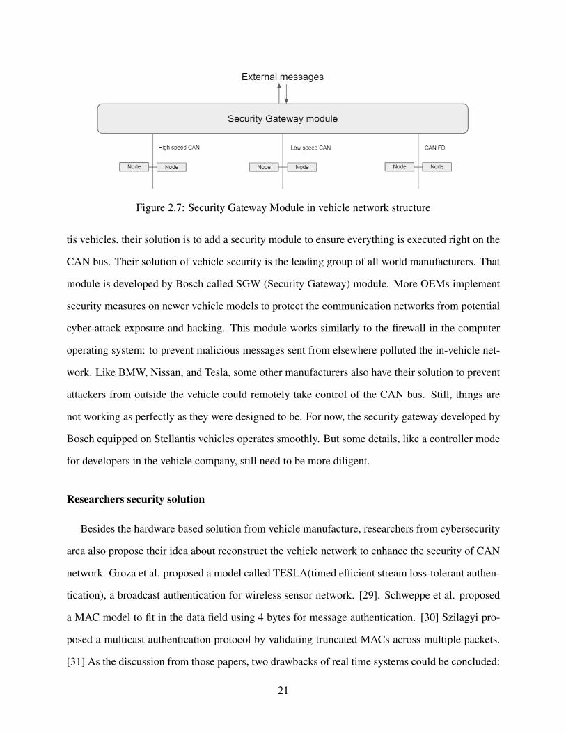
Figure 2.7: Security Gateway Module in vehicle network structure

tis vehicles, their solution is to add a security module to ensure everything is executed right on the

CAN bus. Their solution of vehicle security is the leading group of all world manufacturers. That

module is developed by Bosch called SGW (Security Gateway) module. More OEMs implement

security measures on newer vehicle models to protect the communication networks from potential

cyber-attack exposure and hacking. This module works similarly to the firewall in the computer

operating system: to prevent malicious messages sent from elsewhere polluted the in-vehicle net-

work. Like BMW, Nissan, and Tesla, some other manufacturers also have their solution to prevent

attackers from outside the vehicle could remotely take control of the CAN bus. Still, things are

not working as perfectly as they were designed to be. For now, the security gateway developed by

Bosch equipped on Stellantis vehicles operates smoothly. But some details, like a controller mode

for developers in the vehicle company, still need to be more diligent.

Researchers security solution

Besides the hardware based solution from vehicle manufacture, researchers from cybersecurity

area also propose their idea about reconstruct the vehicle network to enhance the security of CAN

network. Groza et al. proposed a model called TESLA(timed efficient stream loss-tolerant authen-

tication), a broadcast authentication for wireless sensor network. [29]. Schweppe et al. proposed

a MAC model to fit in the data field using 4 bytes for message authentication. [30] Szilagyi pro-

posed a multicast authentication protocol by validating truncated MACs across multiple packets.

[31] As the discussion from those papers, two drawbacks of real time systems could be concluded:

21

1. There is no validation at the beginning of receiving all messages transmitted on the CAN bus.

2. Real time systems could increase the message processing time and that may be the hotbed for

the DoS(deny of service) [32] attack.

22

Chapter 3

System Requirements

To build a complete mapper tool, we need to follow the requirements listed below to make

sure every function meets our aim of the system: an inclusive, stable, and efficient under multi-

platform data collection environment. And this chapter will be divided into the mapper algorithm

type choosing, mapper tool design requirement, and the requirement of time and space complexity.

3.1 Choose A Mapper Algorithm Type

We aim to gather mapping information about the in-vehicle network. Each ECU or function

has its characteristic, and this characteristic could be hardware characteristic, network character-

istic, etc. The mapping tool needs to utilize those characteristics to differentiate ECU function

to recognize the network ECU function. Two kinds of CAN bus features are frequently used as

the grouping algorithm design. The first one is voltage characteristic, and the second one is time

characteristic.

Voltage-based

Different electric signals from the same ECU travel have the same electrical parameters since

those signals originated from the exact location. But for modules from multiple areas, the message

voltage will be different. And also, the ECU wear will cause the electric connection not to be as

good as brand new, and it will impact the signal’s voltage. So, a voltage-based algorithm could be

established based on the hardware characteristic of the electronic nodes.

23

Time-based

The other way to demonstrate the CAN network on a vehicle is to use the time information,

including time skew and deviation. Time skew is the difference between the frequencies of the

predefined and designed clock and the actual clock. Time deviation is the difference between the

real clock and the scheduled time after a certain period. So we can utilize the time information

carried by the CAN message to formulate our mapping tool.

After comparison, the time-based design will be more inclusive (Every CAN will carry the

time information the ECU generates), more fault tolerance (Time will be influenced more minus-

cule than the voltage under different temperature, moisture situations). Voltage-based information

should be more accurate and faster to analyze.

3.2 Time complexity and Space complexity requirement

Space complexity: For asynchronous mapper, there is no particular requirement since all the

Data is processed offline, so the space complexity is O(n). But for the real-time ECU mapper,

although the space complexity is stillO(n), we need to make sure the algorithm meets the hardware

requirement. First, space complexity should allow the algorithm to run on a mainstream micro-

controller board like the table 3.1, which shows the mainstream board flash memory for the ST

board. That storage capacity for the micro-controller will limit the speed of logging and may

influence the result. So, the space complexity needs to match the storage capacity of the micro-

controller to avoid missing the data.

Time complexity: Asynchronous mapper tool should limit time complexity to O(n2). Time

complexity will also be the same for synchronous mapper as asynchronous mapper: O(n2). The

time complexity should meet the need for flashing speed. For ST board like table 3.1, the running

process time should not exceed the time for the micro-controller board collecting the flash memory

amount of data, which is 2MB. If the running time is too long, although that is multi-thread, it

would still influence the processing of sniffing data as the sniffing process is power cost. As the

size data become more significant, it will extend time complexity by squaring. So, the mapper tool

24

should limit the time complexity by limiting the size of processing data.

Peripheral STM32G seiries STM32F series STM32 nucleoMax Flash Memory 2MB 2MB 2MB

Table 3.1: Normal boards flash memory from ST company

3.3 Mapping tool structure

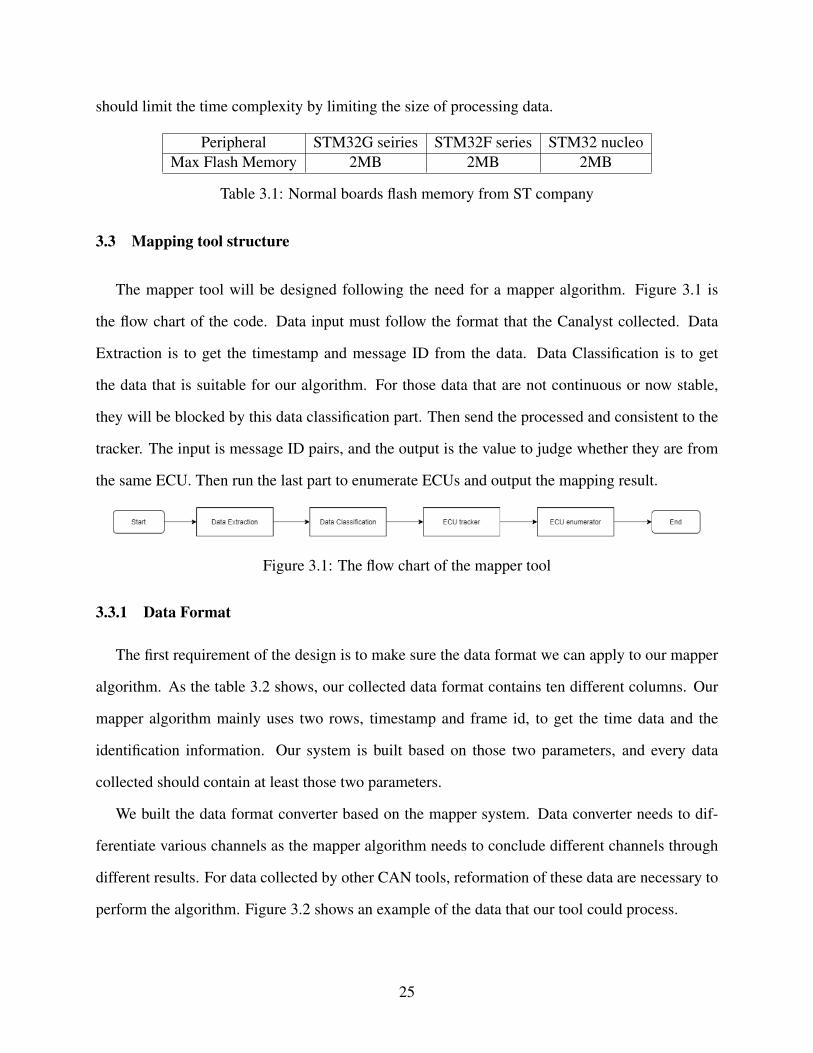
The mapper tool will be designed following the need for a mapper algorithm. Figure 3.1 is

the flow chart of the code. Data input must follow the format that the Canalyst collected. Data

Extraction is to get the timestamp and message ID from the data. Data Classification is to get

the data that is suitable for our algorithm. For those data that are not continuous or now stable,

they will be blocked by this data classification part. Then send the processed and consistent to the

tracker. The input is message ID pairs, and the output is the value to judge whether they are from

the same ECU. Then run the last part to enumerate ECUs and output the mapping result.

Figure 3.1: The flow chart of the mapper tool

3.3.1 Data Format

The first requirement of the design is to make sure the data format we can apply to our mapper

algorithm. As the table 3.2 shows, our collected data format contains ten different columns. Our

mapper algorithm mainly uses two rows, timestamp and frame id, to get the time data and the

identification information. Our system is built based on those two parameters, and every data

collected should contain at least those two parameters.

We built the data format converter based on the mapper system. Data converter needs to dif-

ferentiate various channels as the mapper algorithm needs to conclude different channels through

different results. For data collected by other CAN tools, reformation of these data are necessary to

perform the algorithm. Figure 3.2 shows an example of the data that our tool could process.

25

Column ExplanationIndex The index of the collected data counting from 0System Time Time information generated by the data logging toolTime Stamp Time information included inside the CAN messages frameChannel Shows which channel on the dual channel CAN bus on vehicleDirection Two direction: transmit by the CAN tool or receive by the CAN toolFrame ID CAN message identification numberType The CAN frame type. The type is Data in our data collectionFormat The CAN frame format. Standard CAN bus message is neededDLC The length of the data block inside the CAN frameData Data block in the CAN frame

Table 3.2: Collected data format

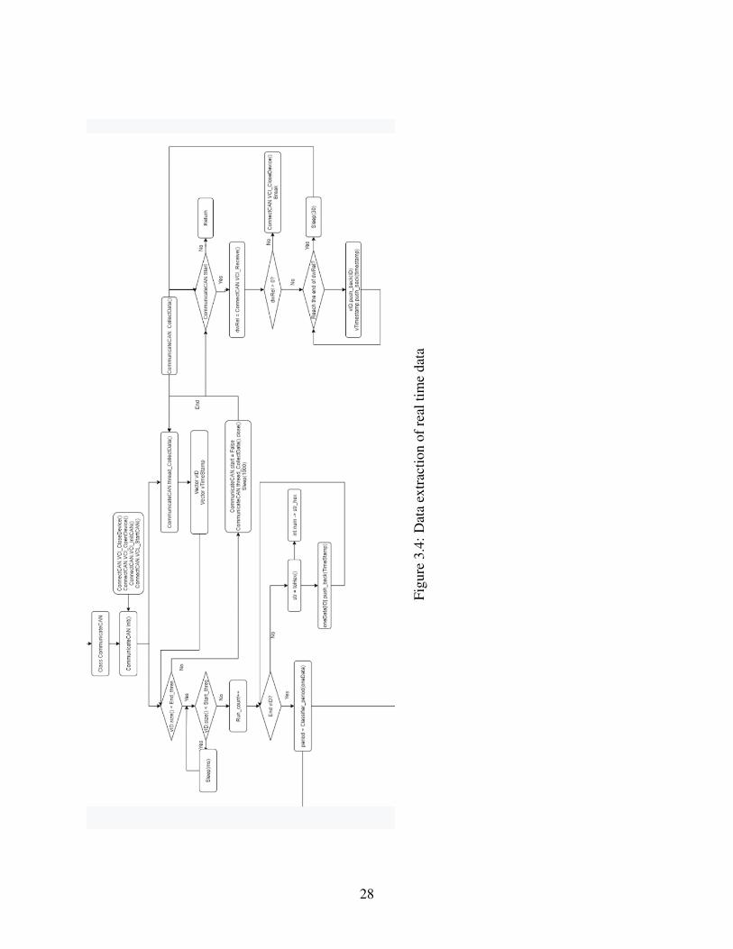
3.3.2 Data Extraction

Data extraction contains read-from-the-file data source and real-time data source using Canalyst

data source. Read-data-from-the-file data is relatively easy, and extraction only needs to realize the

functionality of gathering the information of identification number and time stamp and store them

in the C++ Vector parameter oneData as the flow chart figure 3.3 shows.

We need to call the built-in function in the Canalyst data sniffing tool based on the C++ platform

for real-time data. The flow chart figure 3.4 introduces real-time data processing. The first step

is to establish the communication of the Canalyst tool and the computer by calling the Connect-

CAN.VCI() API is defined in the Canalyst device. First, the processing method and the collecting

method need to run simultaneously, which requires us to set up the multithread function in C++ to

keep two processes running simultaneously. A buffer exists in the CAN sniffing tool that allows us

to store part of the data in the device first then send a pack of data back to the computer to process.

Between each transmission to the computer, sleeping time is set to 30ms to keep the buffer not

overflowing. Each pack will be inserted to the data collection vector and processed.

26

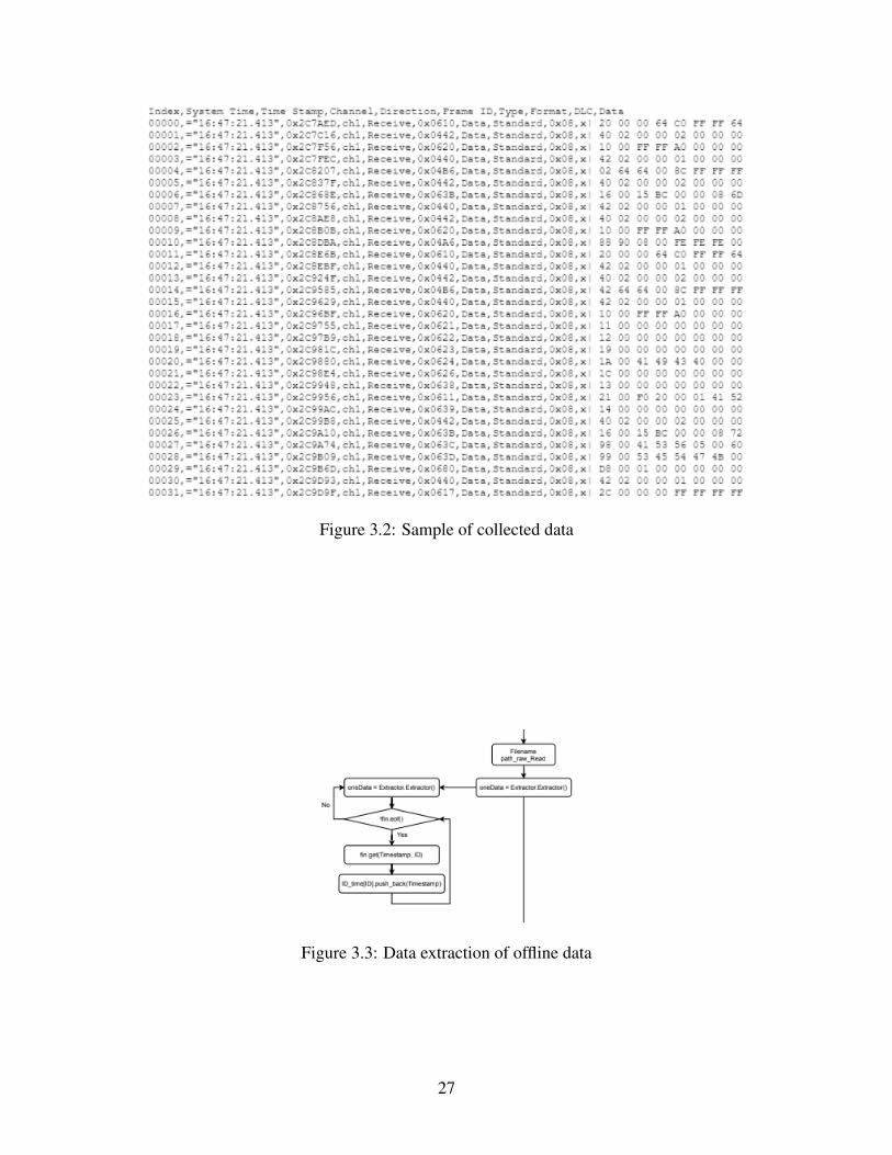
Figure 3.2: Sample of collected data

Figure 3.3: Data extraction of offline data

27

Figu

re3.

4:D

ata

extr

actio

nof

real

time

data

28

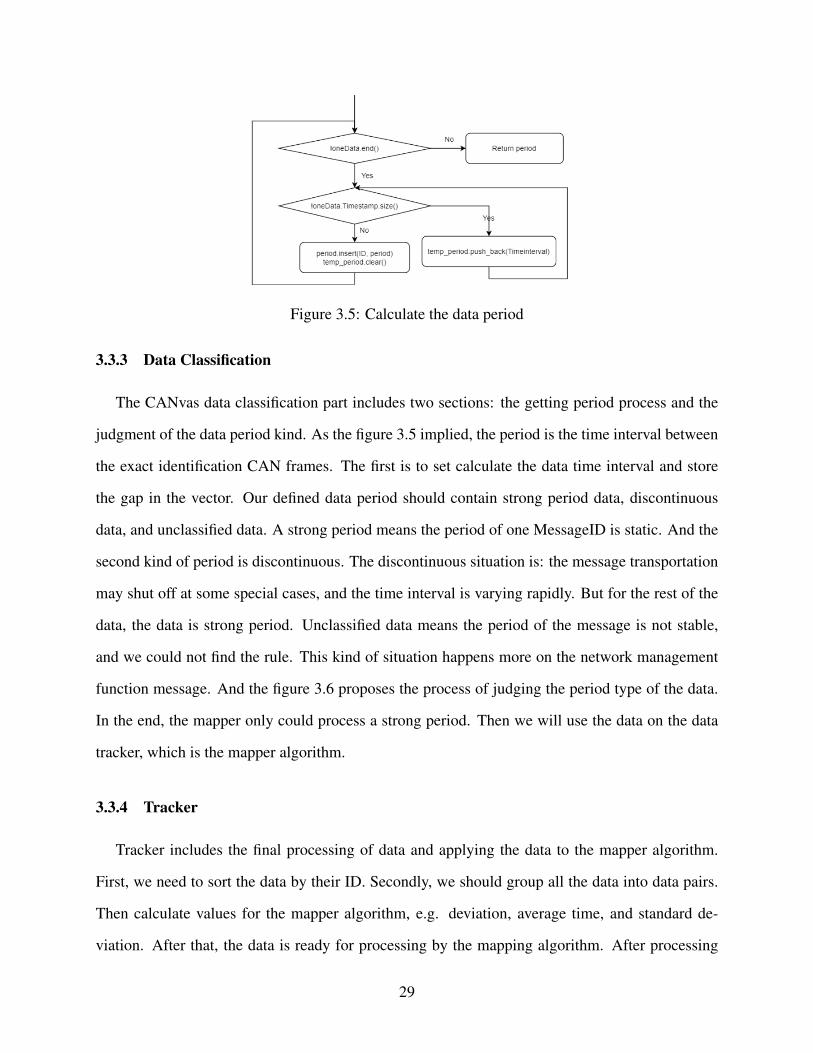
Figure 3.5: Calculate the data period

3.3.3 Data Classification

The CANvas data classification part includes two sections: the getting period process and the

judgment of the data period kind. As the figure 3.5 implied, the period is the time interval between

the exact identification CAN frames. The first is to set calculate the data time interval and store

the gap in the vector. Our defined data period should contain strong period data, discontinuous

data, and unclassified data. A strong period means the period of one MessageID is static. And the

second kind of period is discontinuous. The discontinuous situation is: the message transportation

may shut off at some special cases, and the time interval is varying rapidly. But for the rest of the

data, the data is strong period. Unclassified data means the period of the message is not stable,

and we could not find the rule. This kind of situation happens more on the network management

function message. And the figure 3.6 proposes the process of judging the period type of the data.

In the end, the mapper only could process a strong period. Then we will use the data on the data

tracker, which is the mapper algorithm.

3.3.4 Tracker

Tracker includes the final processing of data and applying the data to the mapper algorithm.

First, we need to sort the data by their ID. Secondly, we should group all the data into data pairs.

Then calculate values for the mapper algorithm, e.g. deviation, average time, and standard de-

viation. After that, the data is ready for processing by the mapping algorithm. After processing

29

by the mapping algorithm, we can apply the mapper algorithm result to the enumeration part to

summarize the result.

3.3.5 Enumeration

The last part of the CANvas is the enumeration. The enumeration aims to gather the output of

the grouping algorithm and enumerate the mapper result. In our mapper algorithm, all output re-

sults are the correlation coefficient of message pairs. Those message pairs may have intersections.

So, we need to extract those intersections and clarify the result.

The process before enumerating is to sort the mapper algorithm by message IDs. During the

enumeration, the first step is to set the aim to enumerate ID1 and find all grouped message pairs

that contain ID1. That is the initial enumeration result of one enumerated result ECU. Then for

each messages pair not enumerated, we follow the same procedure and add new messages in that

group. For new pairs we have not included, add the new messages pair to a new group. Each group

is named ECU 1 to end, but it represents the results of the mapper.

3.3.6 End

After all those steps, we can get the source mapping result.

30

Figure 3.6: Judgment of the data period

31

Chapter 4

Source Mapper Design and Improvements

In this Chapter, we introduce and test three new source mapping algorithm designs: (1) CAN-

vas+, an improved version of CANvas [10]; (2) machine-learning (KNN and DBSCAN) based

grouping; (3) Covariance.

4.1 CANvas+

CANvas is a vehicle network mapper that could meet the requirements of two main outputs

which are source mapping and destination mapping. Source mapping is based on the transmitting

ECU for each unique CAN message and the destination message is based on the set of receiving

ECUs for each unique CAN message. In this paper, We only focus on the transmitting ECU for

each unique CAN message.

4.1.1 CANvas Algorithm

CANvas algorithm is a time based mapper algorithm. In the algorithm, all messages processed

need to be grouped under a certain time window to make the mapping result more accurate. CAN-

vas uses the LCM(Least Common Multiplication) method to generate a proper time window. After

this, we can get the group X: x1, x2...xn and Y : y1, y2...yn. CANvas needs to calculate the group

time deviation DX , DY for each item in X , Y . DX and DY include all the time deviation value

within their groups. For each item Dxi, Dyi in DX , DY , we find the difference value between

Dxi and Dyi. Then store the difference value into data array D. The final step is to calculate the

standard deviation value θ of the array D. If the standard deviation θ below the threshold, CANvas

32

will recognize those two messages from the same ECU. If not, they are not from the same ECU.

4.1.2 CANvas+ Algorithm

The CANvas algorithm has limitation from accuracy and adaptability perspective as we men-

tioned. Due to the limitation of the CANvas, we improve the CANvas method, which we named

CANvas+. This work is initially done by CANvas [10] written in Python. Our work on the LCM

mapper method improves the method by adding more parameters to make the mapper process

more efficient and accurate. For further analysis and adaptability, the LCM method uses c++ code.

C++-based will be quicker and lighter and will contribute a lot to our real-time data collection

and real-time ECU mapping. Since the LCM method is not one main focus, implementing the

algorithm is not contained in this thesis.

We should define several essential parameters first. The divisor value for each group generated

by the LCM method could determine the number of messages in one group. The standard deviation

value for the time offset is the threshold of the grouping method judging whether those messages

are from the same module. By changing those values, we can increase the precious of the mapper

algorithm. Our improvement of the CANvas includes four parts, including divisor value modi-

fication, standard deviation threshold modification, unqualified messages reuse, and similar time

interval message group define.

Divisor value modification

Before calling the LCM algorithm, the function will make sure the divisor number meets the

least qualification. In the paper, (the divisor value is 10), which means we must have ten groups

to call the LCM algorithm. For most data sets, that is an impossible mission. To solve this to get

a more general result, somehow loosen the restriction should work. When the divisor value goes

down, the number of ECU it could map out will be less. Under collective effect on the data result,

we decrease the divisor value to allow more ECU messages under processing.

33

Standard deviation threshold modification

When the algorithm generates the results, the standard deviation threshold will lead to the out-

come. The paper used a threshold of 0.001, and there’s no clue how the author derives this thresh-

old. When the threshold grows more prominent, the result will shake more and contains more

IDs. When the threshold rises to an enormous enough value, like 0.025, the ECU mapping result

won’t change. For example, the dashboard simulator will have at most 5 ECUs. The threshold

author used will be good for the extreme accuracy but not for the general purpose. To balance the

accuracy and generalization, we slightly increase the standard deviation value.

Unqualified messages reuse

For some data thrown out by the divisor, we can reuse it and get it back to the algorithm in a

less accurate way to allow more messages to get in. When the group size is more precise, the group

size will be much more significant. For example, message one average time interval is 0.14578,

and message two average time interval is 0.28444. If we set the effective number to 4, the LCM

of the time interval would be 414.6552. If we are fuzzy the effective number to 3, the LCM of

time interval would be 41.464. So, there will be fewer data needed to get the result. That is good

because when two messages LCM is so huge that some message pairs even need several days of

data to get an unrealistic outcome. Reuse those thrown messages could relieve this situation.

So our solution is to run the algorithm with all the parameters value default and get the first

output set. And for those data that cannot get in the algorithm, rerun the algorithm with modified,

loosen effective number value, and get a new output. Then combine those outputs and get the

result.

Definition of Similar time interval message group

Some similar time interval messages are the breakthrough of the group size difference. When

defining the size of the group of different messages, we can see the influence on the result when

the group size is different. And as the group size grows more significant, the standard deviation

34

will be smaller. Our improvement is to adjust the group size value and proper fit with the standard

deviation threshold value. The influence on the final value is not that large compared with the

parameters mentioned above, but it still could increase the accuracy of the mapper algorithm.

Summary

After all the improvements, the mapping result could meet the need of mapping out the vehicle

network ECUs(factor data result demonstration here). But the algorithm still has two limitations:

1. The CANvas ECU mapping focuses too much on isolating different modules rather than the

responsibility of each module taken. That will lead to the vibration of the result, so we are consid-

ering a more generalized mapper algorithm. 2. LCM method is too approximate, and the threshold

varies heavily for different vehicle environments. In CANvas paper, they got a pretty good result

on a 2008 Toyota Prius. But using the parameters they provide, it is impossible to get a result as

good as they fed. That leads us to test a more generalized, network function-oriented algorithm

mapper algorithm.

4.2 Machine Learning Based Source Mapping

Clustering method - The machine learning method in this thesis is not our primary job. Since the

mapping algorithm shares the same idea with the clustering design in machine learning, we apply

our data to the unsupervised learning clustering algorithm. For now, two trending algorithm, one

is KNN(K nearest neighbors algorithm) [27], [33], [34] and the other is DBSCAN (density-based

spatial clustering) [35], [36]. KNN algorithm finds the nearest number of k points and speculates

those points are from which cluster. Then the new point has more chance to belong to that cluster.

DBSCAN is a clustering algorithm that could reflect the recursion idea: when we first set one point

as cluster number one, we need to write a circle around the first point to find the next point inside

the circle points to the same cluster. We will also write the same size circle around them for all

new points in that circle to find the next points. The same procedure will sustain until no new point

joins in.

35

Implementation - After initial testing, we decide to use the DBSCAN algorithm. Several com-

binations of the time parameters serve as the input of the machine learning algorithm. The first

parameter is the average time deviation, which is the mean value of the time deviation value from

each group. The second parameter is the correlation value and the correlation coefficient calculated

from the Covariance method. Two messages with different IDs are tested each time for parameters

Covariance value and correlation coefficient. Then repeat the same step until covering all mes-

sages. We only finish initial tests on the DBSCAN algorithm, so it does not perform as well as the

Covariance and LCM methods. These prior leads us to do the covariance. Only difference with

CANvas is tracker design.

4.3 Covariance

CANvas inspires us to a new method. We compare messages pairs using the time interval ti

between two messages. The Covariance method is how we calculate the value for identification

whether they are from the same ECU between two messages in one message pair. Moreover, we

develop a new method to deal with the group size replace the LCM method to use fewer data to

generate the result.

4.3.1 Covariance Algorithm

We come up with the method of using the correlation to perform source mapping to improve

the mapping algorithm which we call the Covariance method. The overall idea of this method is:

if messages are from the same ECU, the time interval changing trend of the CAN messages should

be similar, no matter how long the time interval is. The figure 4.1 implies an example about the

messages changing trend from the same ECU. The X-axis is the timeline, and the Y-axis is the

actual time interval value. A is the mean value of the CAN message with a longer time interval,

and K1 is the mean value of the CAN message with a shorter time interval. The dot lines A and

K1 show the mean time interval. Meanwhile, the solid lines are the actual time interval. If two

messages are from the same ECU, their actual time interval changing trend should be similar as the

36

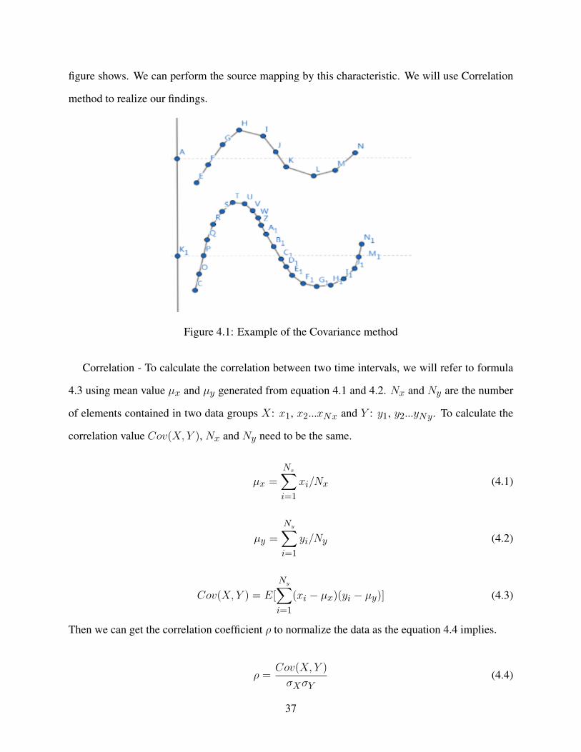
figure shows. We can perform the source mapping by this characteristic. We will use Correlation

method to realize our findings.

Figure 4.1: Example of the Covariance method

Correlation - To calculate the correlation between two time intervals, we will refer to formula

4.3 using mean value µx and µy generated from equation 4.1 and 4.2. Nx and Ny are the number

of elements contained in two data groups X: x1, x2...xNx and Y : y1, y2...yNy. To calculate the

correlation value Cov(X, Y ), Nx and Ny need to be the same.

µx =

Nx∑i=1

xi/Nx (4.1)

µy =

Ny∑i=1

yi/Ny (4.2)

Cov(X, Y ) = E[

Ny∑i=1

(xi − µx)(yi − µy)] (4.3)

Then we can get the correlation coefficient ρ to normalize the data as the equation 4.4 implies.

ρ =Cov(X, Y )

σXσY(4.4)

37

This ρ value reflects the changing trend of the time intervals between two messages. If two mes-

sages are from the same ECU, their ρ value should be close to 1. We cannot determine that when

the ρ value is close to 1, those two messages are from the same ECU. However, we can make sure

those two messages are related to a function block realized on the vehicle’s internal exact location.

Furthermore, it could reflect more on the functional structure of the vehicle. Nevertheless, we

cannot use the time interval of every single message as the ρ value will be too sensitive, and the

system would be inefficient. So, we decided to import the time window to group several messages

together, which the CANvas does the same.

Time window - As we mentioned before, the CANvas mapper used the LCM method, which

disadvantages the group size. So, we decided to set the window size to a fixed value to avoid these

flaws. This value should be adjusted to a specific value to keep the accuracy for general vehicles.

Also, we need some process for handling the edge since the endpoint of the time window may not

be at the time point of the message. The parameter we will use for the Covariance method is the

time interval value of the time window. We will find the changing trend of the time window of two

messages to find whether they are from the same function block.

Then, we can process the enumeration part to get the source mapping result. That is the basic

idea of our algorithm. Then we will discuss details about how we realize our algorithm.

4.3.2 Relevant Parameters Definition

Table 4.1 shows the parameters and their definitions we use for this section.

Group definition - Figure 4.2 shows how to figure out the message groups. Suppose ID1 and ID2

are ID pairs we need to compare. All parameters are defined as Table 4.1 shows. Note that Tx: tx0,

tx1...txn contains the average time interval plus the time deviation accumulated. Sometimes time

deviation values are positive and sometimes are negative. For most cases, M and N parameters

are not integers.

Time window definition - Time window is the difference value between parameter Gis and

Gie. We must deal with data pairs that include long time intervals and short time intervals. The

38

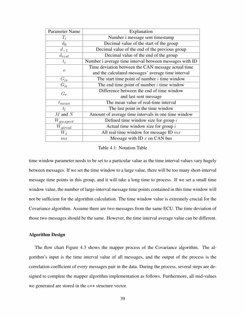
Parameter Name ExplanationTi Number i message sent timestampd0 Decimal value of the start of the groupd−1 Decimal value of the end of the previous groupdrest Decimal value of the end of the groupti Number i average time interval between messages with ID

oTime deviation between the CAN message actual time

and the calculated messages’ average time intervalGis The start time point of number i time windowGie The end time point of number i time window

GrDifference between the end of time window

and last sent messagetmean The mean value of real-time intervaltl The last point in the time window

M and N Amount of average time intervals in one time windowWgiexpect Defined time window size for group iWgireal Actual time window size for group iWx All real time window for message ID mxmx Message with ID x on CAN bus

Table 4.1: Notation Table

time window parameter needs to be set to a particular value as the time interval values vary hugely

between messages. If we set the time window to a large value, there will be too many short-interval

message time points in this group, and it will take a long time to process. If we set a small time

window value, the number of large-interval message time points contained in this time window will

not be sufficient for the algorithm calculation. The time window value is extremely crucial for the

Covariance algorithm. Assume there are two messages from the same ECU. The time deviation of

those two messages should be the same. However, the time interval average value can be different.

Algorithm Design

The flow chart Figure 4.3 shows the mapper process of the Covariance algorithm. The al-

gorithm’s input is the time interval value of all messages, and the output of the process is the

correlation coefficient of every messages pair in the data. During the process, several steps are de-

signed to complete the mapper algorithm implementation as follows. Furthermore, all mid-values

we generated are stored in the c++ structure vector.

39

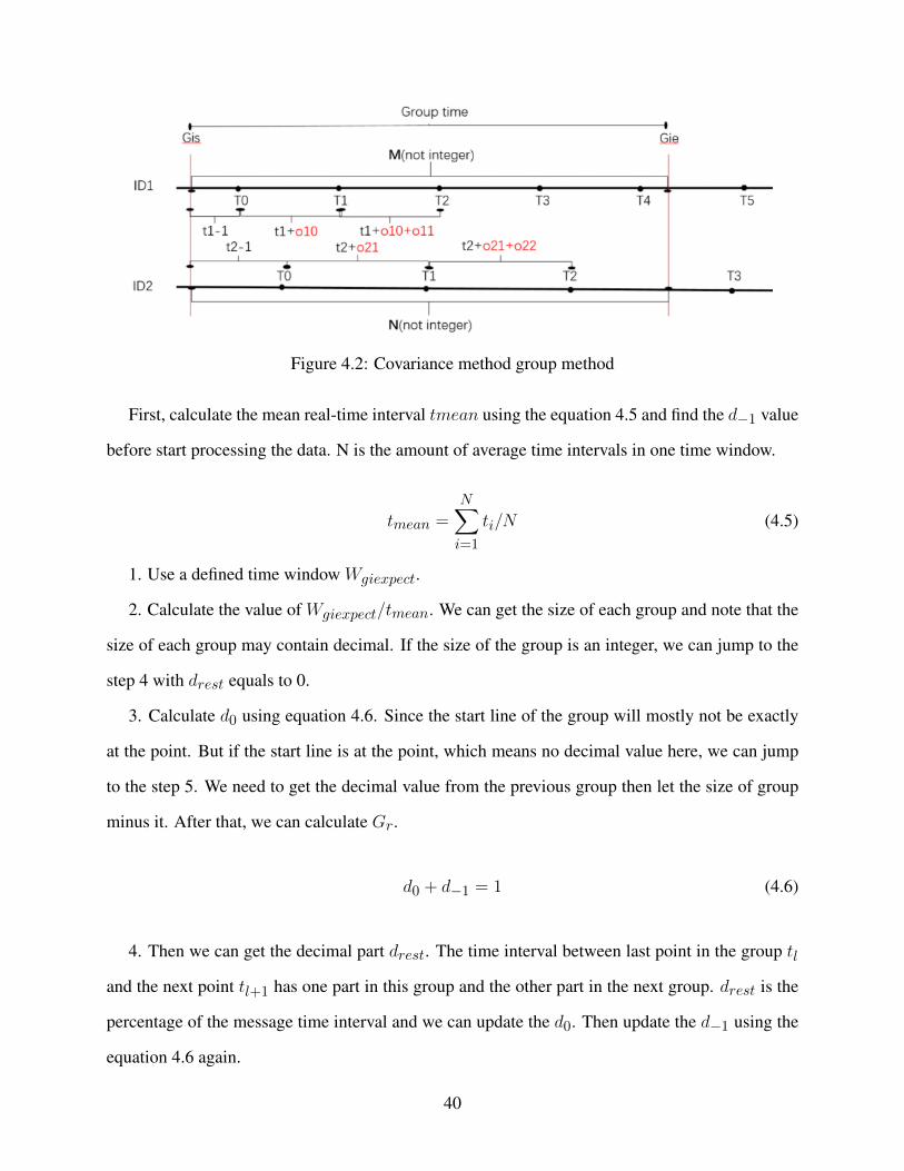
Figure 4.2: Covariance method group method

First, calculate the mean real-time interval tmean using the equation 4.5 and find the d−1 value

before start processing the data. N is the amount of average time intervals in one time window.

tmean =N∑i=1

ti/N (4.5)

1. Use a defined time window Wgiexpect.

2. Calculate the value of Wgiexpect/tmean. We can get the size of each group and note that the

size of each group may contain decimal. If the size of the group is an integer, we can jump to the

step 4 with drest equals to 0.

3. Calculate d0 using equation 4.6. Since the start line of the group will mostly not be exactly

at the point. But if the start line is at the point, which means no decimal value here, we can jump

to the step 5. We need to get the decimal value from the previous group then let the size of group

minus it. After that, we can calculate Gr.

d0 + d−1 = 1 (4.6)

4. Then we can get the decimal part drest. The time interval between last point in the group tl

and the next point tl+1 has one part in this group and the other part in the next group. drest is the

percentage of the message time interval and we can update the d0. Then update the d−1 using the

equation 4.6 again.

40

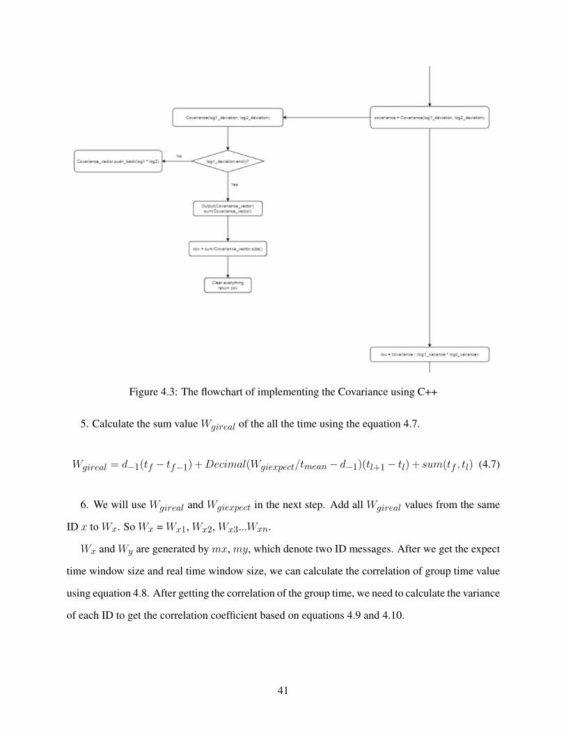
Figure 4.3: The flowchart of implementing the Covariance using C++

5. Calculate the sum value Wgireal of the all the time using the equation 4.7.

Wgireal = d−1(tf − tf−1) +Decimal(Wgiexpect/tmean− d−1)(tl+1− tl) + sum(tf , tl) (4.7)

6. We will use Wgireal and Wgiexpect in the next step. Add all Wgireal values from the same

ID x to Wx. So Wx = Wx1, Wx2, Wx3...Wxn.

Wx and Wy are generated by mx, my, which denote two ID messages. After we get the expect

time window size and real time window size, we can calculate the correlation of group time value

using equation 4.8. After getting the correlation of the group time, we need to calculate the variance

of each ID to get the correlation coefficient based on equations 4.9 and 4.10.

41

Cov(mx,my) =1

n

n∑i=1

(Wxi −Wgiexpect)(Wyi −Wgiexpect) (4.8)

σ2mx =1

n

n∑i=1

(Wxi −Wgiexpect)2 (4.9)

σ2my =1

n

n∑i=1

(Wyi −Wgiexpect)2 (4.10)

Finally we can get the ρ we need for further comparison using equation 4.11.

ρ =cov(mx,my)

σmxσmy(4.11)

We can evaluate the activity of two messages based on the ρ we derived. If two IDs vary in the

same way, the ρ value would be 1. If those two IDs vary differently, the ρ value would be -1, which

would not happen. A threshold needs setting to evaluate whether they are from the same ECUs.

That is our new Covariance algorithm that could increase the accuracy by defining the ρ value.

As the experiment’s group size is defined, we do not need massive data to get an output. That

algorithm could meet the need for accuracy and data size as the requirement analysis introduced

above. After this, we can apply the ensured data pairs to the enumerate method to output the ECU

mapping result.

4.3.3 Covariance Improvement

Mapper tool improvement includes some pre-process improvement before applying Covariance

mapping algorithms and the improvement for the Covariance methods. Pre-process improvement

includes the same module characteristic test and the introduction of normalized average real-time

interval parameter. Although the algorithm meets the requirement, things are different when ap-

plying the Covariance mapper tool to a sophisticated modern vehicle. The in-vehicle network will

be highly complicated designed for multi-function, accuracy, and anti-intrusion. Also, some sim-

42

ilar platform ECU hardware will cause minor deviation to the timestamp, which will confuse our

software. So, some further improvements need to be added to help improve the algorithm.

Normalized Average Real-time Interval

Before applying the Covariance mapping algorithm, the normalized average real-time interval

could work as a new parameter for initial time interval processing. That parameter could give us a

basic idea of the vehicle network’s mapping condition and its functionality.

Average real-time interval - When CAN communication messages transmit in the CAN bus, the

transmission time interval is set to a pre-defined value by the manufacturer. Due to the hardware

characteristic, there will be a time offset between the messages. So, the real-time interval T means

the pre-defined time interval plus the time offset. This value would vary when collecting messages

from different modules, but it will remain relatively stable inside a group. The average real-time

interval Tm is the average value of all the real-time intervals in one dataset. In this file, we set the

precision value to 0.0000001ms.

Normalization - The Normalized average real-time interval – NTm is the average real-time

interval after normalization. This normalization process follows our designed self-normalization

method, which will finally restrict the actual average time to 1 second as a standard to make it

easier for comparison. Most car manufacturers will design the message time intervals to an integer

with multiples of 10, 100 values that will not contain 150ms or 1500ms. So, for the time interval

value, we could find the first number that does not equal 0 and approximate the designed time

interval.

NTm =Tm

Nd ∗ 10f(4.12)

Equation 4.12 is how we calculate the normalized average real-time interval value. NTm is the

normalized average real-time interval. Tm is the average real-time interval. Nd is the design-time

interval we approximate from the real value. f is the number of digits before the first number that

is not equal to zero.

Proof - The figure 4.4 shows clearly the time differences between the message IDs and normal-

43

Figure 4.4: Average time from different message IDs that are from same ECU

ized average time. If we draw a horizontal line for one point, the remaining points should be from

the same ECU. To speculate what the normalized average time value represents, we find every ID

function in the manufacturing engineering handbook. Table 4.2 is part of our result for the BCM

module in a 2019 Chrysler Pacifica. We can see from that form, messages with NTm value equals

1.0181946825 mainly focus on the out-of-vehicle cabin control. However, for messages withNTm

value equals 1.0181948413s, it mainly represents the cabin control system.

Same-Module Condition

Same-Module means testing the difference between similar or even identical control modules.

We took LBSS (Left-side blind spot sensor) module and RBSS (Right-side blind spot sensor)

module as our test objects to test the similarity between similar modules. In the bench data test

environment, we test three different network situations, as the figure 4.5 shows. LBSS and RBSS

have similar functionality but different messages. We find that similar blind spot modules, like

RBSS and LBSS, mapping algorithms can not distinguish between them. So, hardware character-

istics are not very obvious for similar modules mounted on different locations in the same vehicle

network. However, since the functionality of those modules is the same, we can conclude them

into one group by grouping the network function using the Covariance method.

44

Message ID Ntm Function0x2C2

1.0181946825s

Suspension system0x381 Transmission system0x39E Hybrid system0x3B3 Handbrake system0x3B4 Back up camera0x3C2 Tire pressure system0x3F4 Wireless control0x3F5 Brake system0x44C Vehicle inspection system(Brake, door, inhale)0x2C6

1.0181948413s

Heated seat0x38A Steering system0x3EA Back door0x3F2 Sounding system0x3F3 Dashboard0x44A Vehicle inspection system(child lock, seat belt)

Table 4.2: Normalized average time value from messages generated by the same module

Figure 4.5: Three conditions for the similar function hardware characteristic test

Unstable data removal

Many factors could cause data instability. This part focuses on the data initialization instability.

Mapper tools need to get rid of those initial data. As the figure 4.6 shows, after deleting the first

several lines of data, the same ECU messages covariance value is reasonable. We used several

different group-size values for comparison. The classifier function will block another part of the

data. Only certified as strong period could reach the tracker part, and we hope to add the dual-

strong period data in the future work since they also meet the design regulation from manufacture.

45

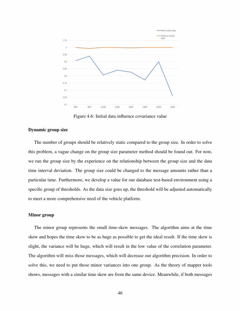
Figure 4.6: Initial data influence covariance value

Dynamic group size

The number of groups should be relatively static compared to the group size. In order to solve

this problem, a vague change on the group size parameter method should be found out. For now,

we run the group size by the experience on the relationship between the group size and the data

time interval deviation. The group size could be changed to the message amounts rather than a

particular time. Furthermore, we develop a value for our database test-based environment using a

specific group of thresholds. As the data size goes up, the threshold will be adjusted automatically

to meet a more comprehensive need of the vehicle platform.

Minor group

The minor group represents the small time-skew messages. The algorithm aims at the time

skew and hopes the time skew to be as huge as possible to get the ideal result. If the time skew is

slight, the variance will be huge, which will result in the low value of the correlation parameter.

The algorithm will miss those messages, which will decrease our algorithm precision. In order to

solve this, we need to put those minor variances into one group. As the theory of mapper tools

shows, messages with a similar time skew are from the same device. Meanwhile, if both messages

46

are close to the expected time, they should also be from the same ECU. There will be a minor

group deviated ECU in our result. That function will make our algorithm more accurate.

47

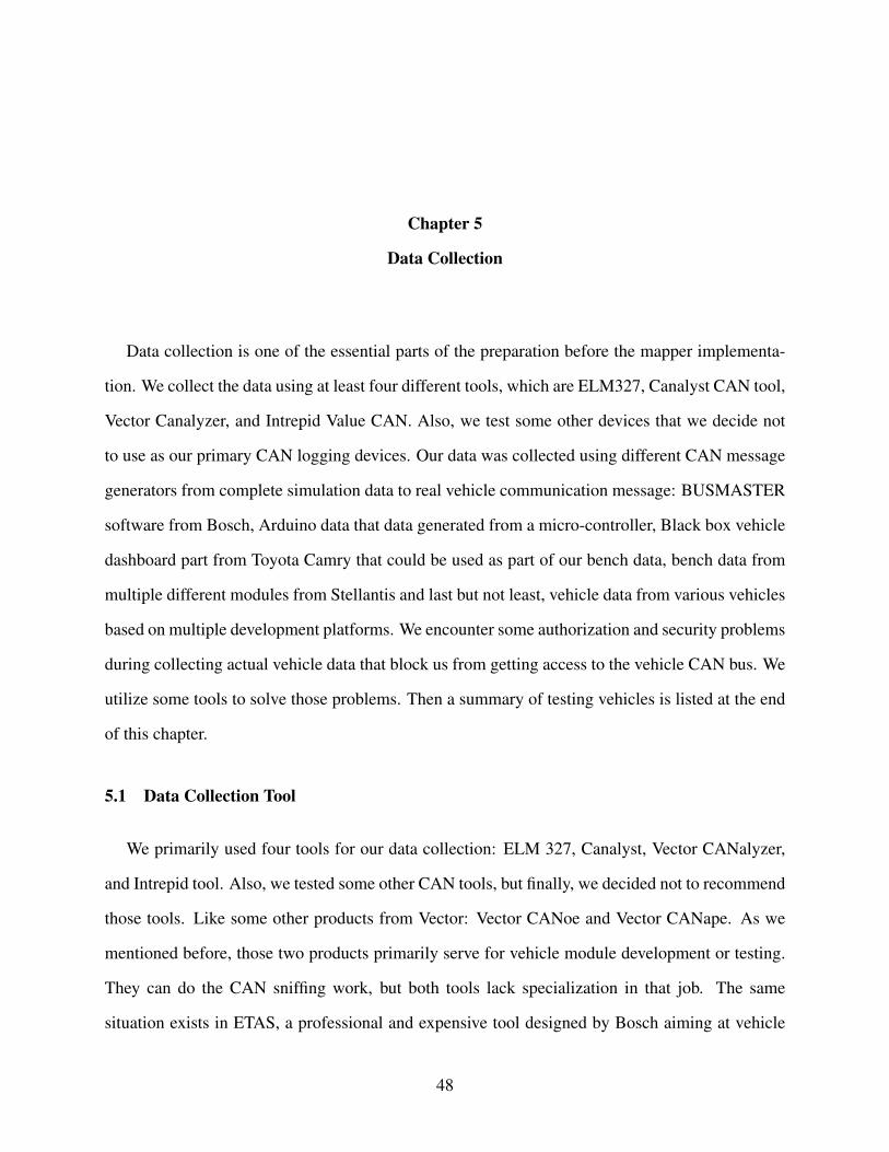
Chapter 5

Data Collection

Data collection is one of the essential parts of the preparation before the mapper implementa-

tion. We collect the data using at least four different tools, which are ELM327, Canalyst CAN tool,

Vector Canalyzer, and Intrepid Value CAN. Also, we test some other devices that we decide not

to use as our primary CAN logging devices. Our data was collected using different CAN message

generators from complete simulation data to real vehicle communication message: BUSMASTER

software from Bosch, Arduino data that data generated from a micro-controller, Black box vehicle

dashboard part from Toyota Camry that could be used as part of our bench data, bench data from

multiple different modules from Stellantis and last but not least, vehicle data from various vehicles

based on multiple development platforms. We encounter some authorization and security problems

during collecting actual vehicle data that block us from getting access to the vehicle CAN bus. We

utilize some tools to solve those problems. Then a summary of testing vehicles is listed at the end

of this chapter.

5.1 Data Collection Tool

We primarily used four tools for our data collection: ELM 327, Canalyst, Vector CANalyzer,

and Intrepid tool. Also, we tested some other CAN tools, but finally, we decided not to recommend

those tools. Like some other products from Vector: Vector CANoe and Vector CANape. As we

mentioned before, those two products primarily serve for vehicle module development or testing.

They can do the CAN sniffing work, but both tools lack specialization in that job. The same

situation exists in ETAS, a professional and expensive tool designed by Bosch aiming at vehicle

48

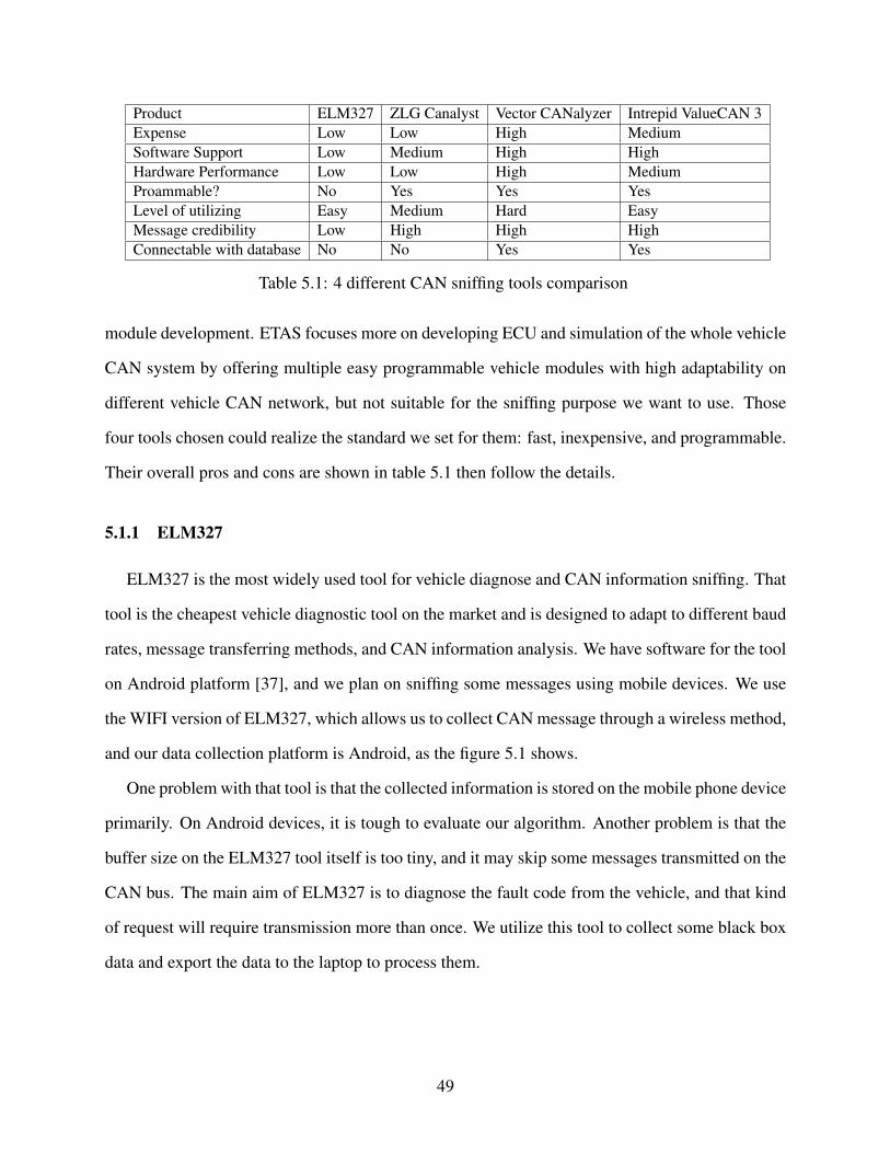
Product ELM327 ZLG Canalyst Vector CANalyzer Intrepid ValueCAN 3Expense Low Low High MediumSoftware Support Low Medium High HighHardware Performance Low Low High MediumProammable? No Yes Yes YesLevel of utilizing Easy Medium Hard EasyMessage credibility Low High High HighConnectable with database No No Yes Yes

Table 5.1: 4 different CAN sniffing tools comparison

module development. ETAS focuses more on developing ECU and simulation of the whole vehicle

CAN system by offering multiple easy programmable vehicle modules with high adaptability on

different vehicle CAN network, but not suitable for the sniffing purpose we want to use. Those

four tools chosen could realize the standard we set for them: fast, inexpensive, and programmable.

Their overall pros and cons are shown in table 5.1 then follow the details.

5.1.1 ELM327

ELM327 is the most widely used tool for vehicle diagnose and CAN information sniffing. That

tool is the cheapest vehicle diagnostic tool on the market and is designed to adapt to different baud

rates, message transferring methods, and CAN information analysis. We have software for the tool

on Android platform [37], and we plan on sniffing some messages using mobile devices. We use

the WIFI version of ELM327, which allows us to collect CAN message through a wireless method,

and our data collection platform is Android, as the figure 5.1 shows.

One problem with that tool is that the collected information is stored on the mobile phone device

primarily. On Android devices, it is tough to evaluate our algorithm. Another problem is that the

buffer size on the ELM327 tool itself is too tiny, and it may skip some messages transmitted on the

CAN bus. The main aim of ELM327 is to diagnose the fault code from the vehicle, and that kind

of request will require transmission more than once. We utilize this tool to collect some black box

data and export the data to the laptop to process them.

49

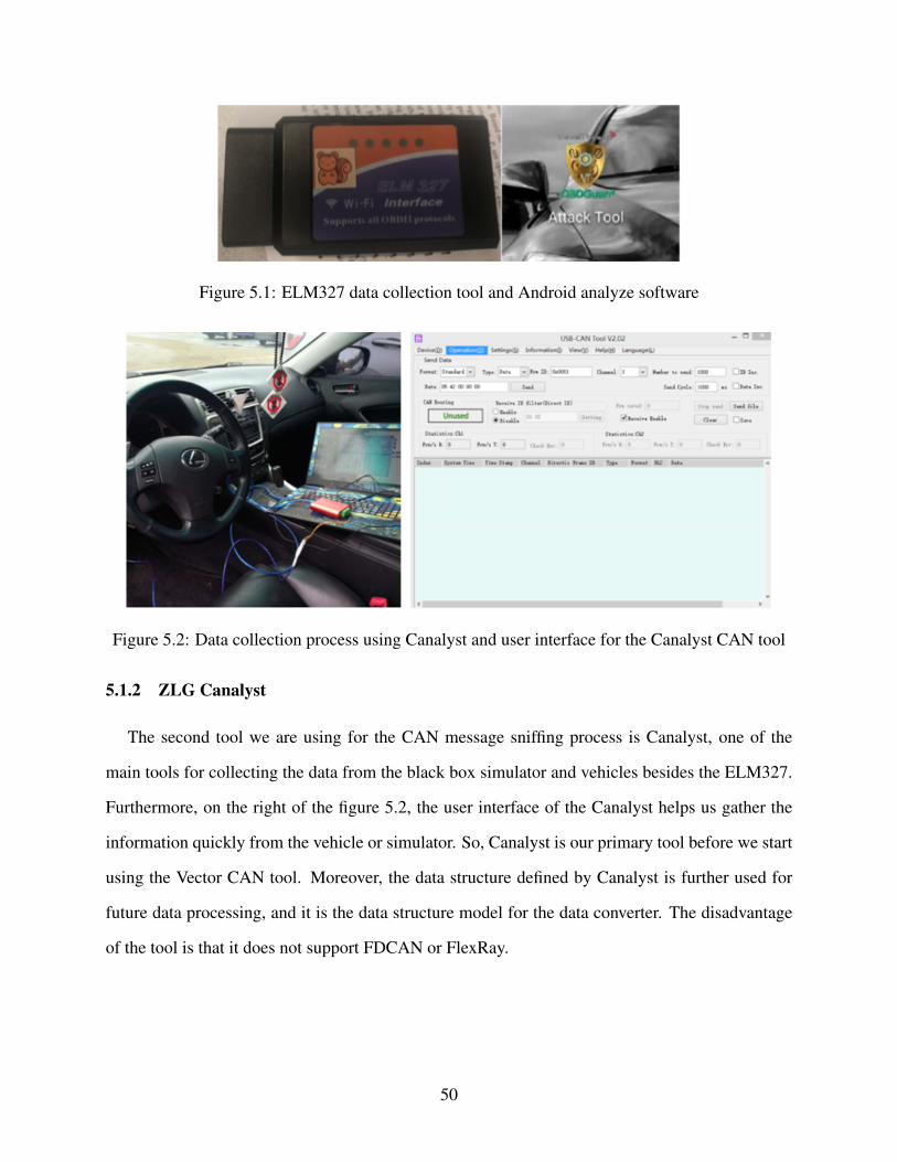
Figure 5.1: ELM327 data collection tool and Android analyze software

Figure 5.2: Data collection process using Canalyst and user interface for the Canalyst CAN tool

5.1.2 ZLG Canalyst

The second tool we are using for the CAN message sniffing process is Canalyst, one of the

main tools for collecting the data from the black box simulator and vehicles besides the ELM327.

Furthermore, on the right of the figure 5.2, the user interface of the Canalyst helps us gather the

information quickly from the vehicle or simulator. So, Canalyst is our primary tool before we start

using the Vector CAN tool. Moreover, the data structure defined by Canalyst is further used for

future data processing, and it is the data structure model for the data converter. The disadvantage

of the tool is that it does not support FDCAN or FlexRay.

50

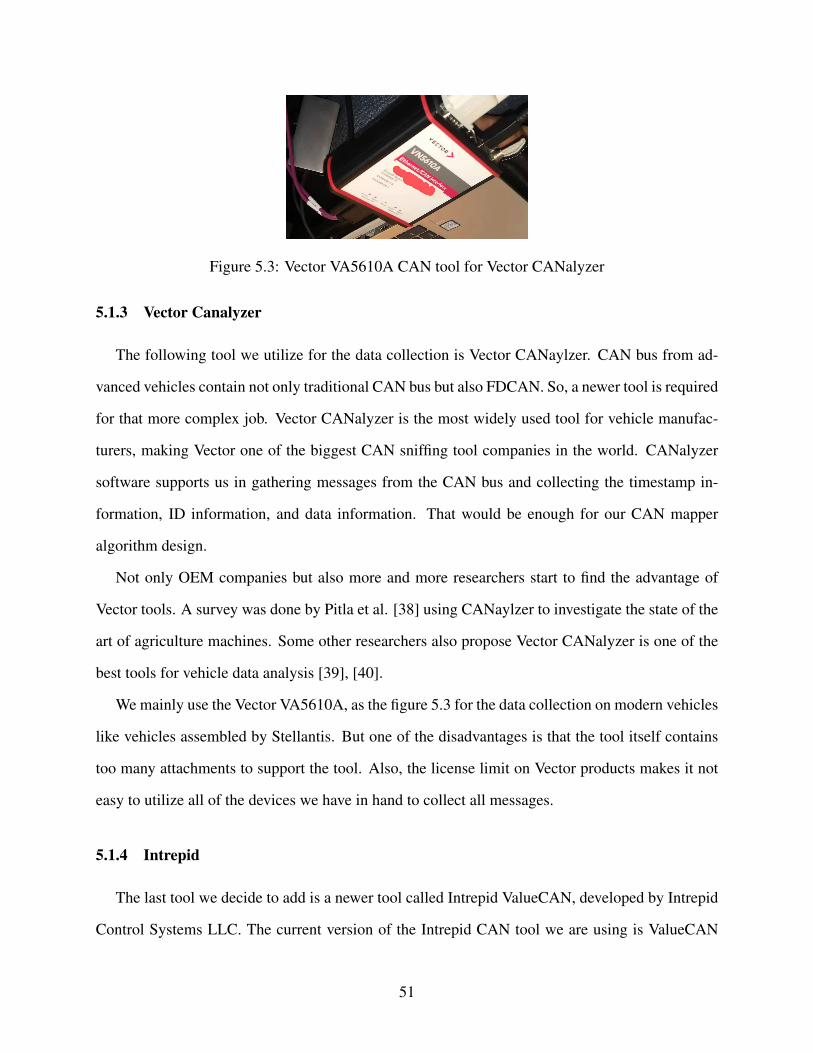
Figure 5.3: Vector VA5610A CAN tool for Vector CANalyzer

5.1.3 Vector Canalyzer

The following tool we utilize for the data collection is Vector CANaylzer. CAN bus from ad-

vanced vehicles contain not only traditional CAN bus but also FDCAN. So, a newer tool is required

for that more complex job. Vector CANalyzer is the most widely used tool for vehicle manufac-

turers, making Vector one of the biggest CAN sniffing tool companies in the world. CANalyzer

software supports us in gathering messages from the CAN bus and collecting the timestamp in-

formation, ID information, and data information. That would be enough for our CAN mapper

algorithm design.

Not only OEM companies but also more and more researchers start to find the advantage of

Vector tools. A survey was done by Pitla et al. [38] using CANaylzer to investigate the state of the

art of agriculture machines. Some other researchers also propose Vector CANalyzer is one of the

best tools for vehicle data analysis [39], [40].

We mainly use the Vector VA5610A, as the figure 5.3 for the data collection on modern vehicles

like vehicles assembled by Stellantis. But one of the disadvantages is that the tool itself contains

too many attachments to support the tool. Also, the license limit on Vector products makes it not

easy to utilize all of the devices we have in hand to collect all messages.

5.1.4 Intrepid

The last tool we decide to add is a newer tool called Intrepid ValueCAN, developed by Intrepid

Control Systems LLC. The current version of the Intrepid CAN tool we are using is ValueCAN

51

Figure 5.4: Intrepid CAN tool for vehicle CAN data collection

3 series, as the figure 5.4 shows. We use the Intrepid CAN tool mainly to collect data from the

bench and the actual vehicle environment. Intrepid also developed a software called Vehicle Spy

to support the ValueCAN tool to monitor the data collection process and store the data in a text

file. The advantage of VauleCAN is the size of the tool itself is relatively tiny and plug-in to use.

The license requirement for that tool is also more friendly for users. The short of the device is

the interface of Vehicle Spy is not very user friendly. In all, that is the perfect tool for our data

collection.

5.2 Data source

We can divide the data source into three different kinds: software-based data, hardware-based

data, and actual vehicle data. Software-based simulation data is to formulate a simulated vehicle

environment in a software or a software-based system to simulate some hardware characteristic.

We mainly use BUSMASTER software from Bosch to gather data like this. And we also use Vector

and ETAS to simulate the in-vehicle environment, but they are not good at mimicking the hardware

characteristic. Then for the hardware-based simulation, we have black box dashboard simulator

data, Arduino microprocessor data, and bench data using modules fitted inside the vehicle. Actual

vehicle data is collected directly through the OBD-II port from vehicles manufactured by Stellantis

and will include Infiniti, Toyota, Nissan, Lexus, and BMW. And the vehicle type will consist of

full-size sedans to heavy-duty trucks, almost every kind of vehicle.

52

Member CAN message identifierisExtended CAN message is extended or notisRtr CAN message is Remote or notdlc Data length in bytescluster Channel on which the frame is receiveddata[64] Message data bytes for CANisCANfd CANFD message or nottimeStamp Frame absolute timestamp

Table 5.2: CAN message builder in BUSMASTER

5.2.1 BUSMASTER Data

BUSMASTER is the software made by Bosch and downloads for free for all users to simulate

the in-vehicle network generally. BUSMASTER allows users to add nodes inside the network and

change that node’s status and function. Multiple functions are pre-defined inside the software.

Table 5.2 shows the parameters specified, like the onBusconnect() function allows users to define

CAN message easily. The figure 5.5 exhibits one of the data we collected, and we can store the

collected data in our computer. Data gathered by BUSMASTER need to be converted to the aim

format.

The disadvantage of the BUSMASTER tool is it can only simulate the hardware characteristic

but could not reflect the actual network condition. Every time deviation of transmitted messages

is following the same pre-defined time cycle. And simulation on the CAN bus’s workload is

unchangeable, making the CAN message time deviation due to the busload eliminated. Second,

BUSMASTER is not open for real-time data processing. But overall, it is good to give us a brief

idea about the algorithm’s feasibility. Data from BUSMASTER will not be our mainly evaluated

object.

5.2.2 Black Box Data

The so-called black box is a vehicle network simulator built based on a 2014 to 2015 Toyota

Camry dashboard. It could simulate almost all the functions an instrument cluster can do. From

figure 5.6, we can see the door lock, radio hub, cluster, and the OBD-II port located inside the

53

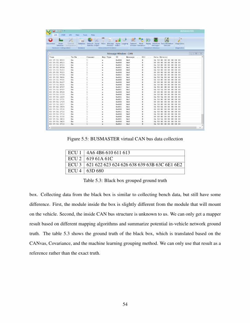
Figure 5.5: BUSMASTER virtual CAN bus data collection

ECU 1 4A6 4B6 610 611 613ECU 2 619 61A 61CECU 3 621 622 623 624 626 638 639 63B 63C 6E1 6E2ECU 4 63D 680

Table 5.3: Black box grouped ground truth

box. Collecting data from the black box is similar to collecting bench data, but still have some

difference. First, the module inside the box is slightly different from the module that will mount

on the vehicle. Second, the inside CAN bus structure is unknown to us. We can only get a mapper

result based on different mapping algorithms and summarize potential in-vehicle network ground

truth. The table 5.3 shows the ground truth of the black box, which is translated based on the

CANvas, Covariance, and the machine learning grouping method. We can only use that result as a

reference rather than the exact truth.

54

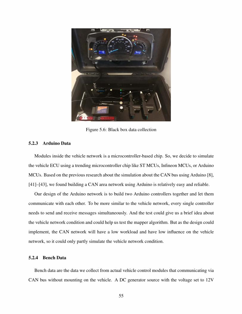
Figure 5.6: Black box data collection

5.2.3 Arduino Data

Modules inside the vehicle network is a microcontroller-based chip. So, we decide to simulate

the vehicle ECU using a trending microcontroller chip like ST MCUs, Infineon MCUs, or Arduino

MCUs. Based on the previous research about the simulation about the CAN bus using Arduino [8],

[41]–[43], we found building a CAN area network using Arduino is relatively easy and reliable.

Our design of the Arduino network is to build two Arduino controllers together and let them

communicate with each other. To be more similar to the vehicle network, every single controller

needs to send and receive messages simultaneously. And the test could give us a brief idea about

the vehicle network condition and could help us test the mapper algorithm. But as the design could

implement, the CAN network will have a low workload and have low influence on the vehicle

network, so it could only partly simulate the vehicle network condition.

5.2.4 Bench Data

Bench data are the data we collect from actual vehicle control modules that communicating via

CAN bus without mounting on the vehicle. A DC generator source with the voltage set to 12V

55

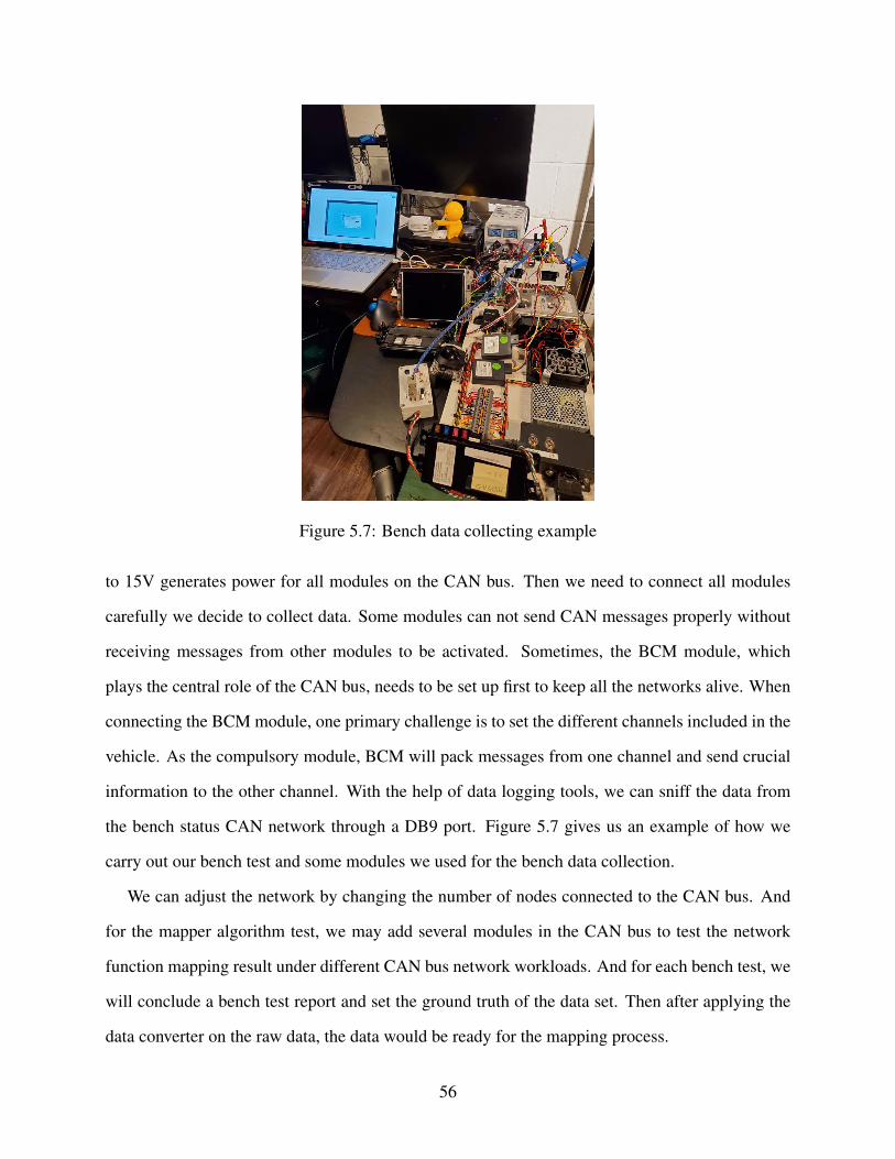
Figure 5.7: Bench data collecting example

to 15V generates power for all modules on the CAN bus. Then we need to connect all modules

carefully we decide to collect data. Some modules can not send CAN messages properly without

receiving messages from other modules to be activated. Sometimes, the BCM module, which

plays the central role of the CAN bus, needs to be set up first to keep all the networks alive. When

connecting the BCM module, one primary challenge is to set the different channels included in the

vehicle. As the compulsory module, BCM will pack messages from one channel and send crucial

information to the other channel. With the help of data logging tools, we can sniff the data from

the bench status CAN network through a DB9 port. Figure 5.7 gives us an example of how we

carry out our bench test and some modules we used for the bench data collection.

We can adjust the network by changing the number of nodes connected to the CAN bus. And

for the mapper algorithm test, we may add several modules in the CAN bus to test the network

function mapping result under different CAN bus network workloads. And for each bench test, we

will conclude a bench test report and set the ground truth of the data set. Then after applying the

data converter on the raw data, the data would be ready for the mapping process.

56

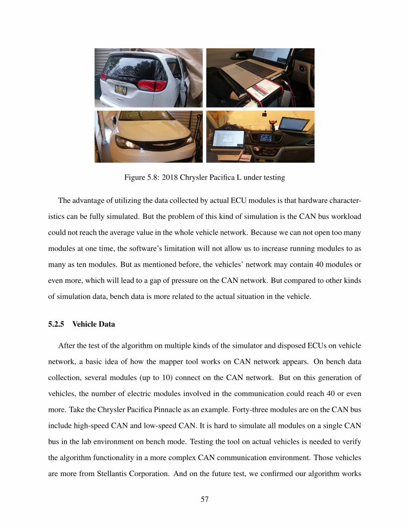
Figure 5.8: 2018 Chrysler Pacifica L under testing

The advantage of utilizing the data collected by actual ECU modules is that hardware character-

istics can be fully simulated. But the problem of this kind of simulation is the CAN bus workload

could not reach the average value in the whole vehicle network. Because we can not open too many

modules at one time, the software’s limitation will not allow us to increase running modules to as

many as ten modules. But as mentioned before, the vehicles’ network may contain 40 modules or

even more, which will lead to a gap of pressure on the CAN network. But compared to other kinds

of simulation data, bench data is more related to the actual situation in the vehicle.

5.2.5 Vehicle Data

After the test of the algorithm on multiple kinds of the simulator and disposed ECUs on vehicle

network, a basic idea of how the mapper tool works on CAN network appears. On bench data

collection, several modules (up to 10) connect on the CAN network. But on this generation of

vehicles, the number of electric modules involved in the communication could reach 40 or even

more. Take the Chrysler Pacifica Pinnacle as an example. Forty-three modules are on the CAN bus

include high-speed CAN and low-speed CAN. It is hard to simulate all modules on a single CAN

bus in the lab environment on bench mode. Testing the tool on actual vehicles is needed to verify

the algorithm functionality in a more complex CAN communication environment. Those vehicles

are more from Stellantis Corporation. And on the future test, we confirmed our algorithm works

57

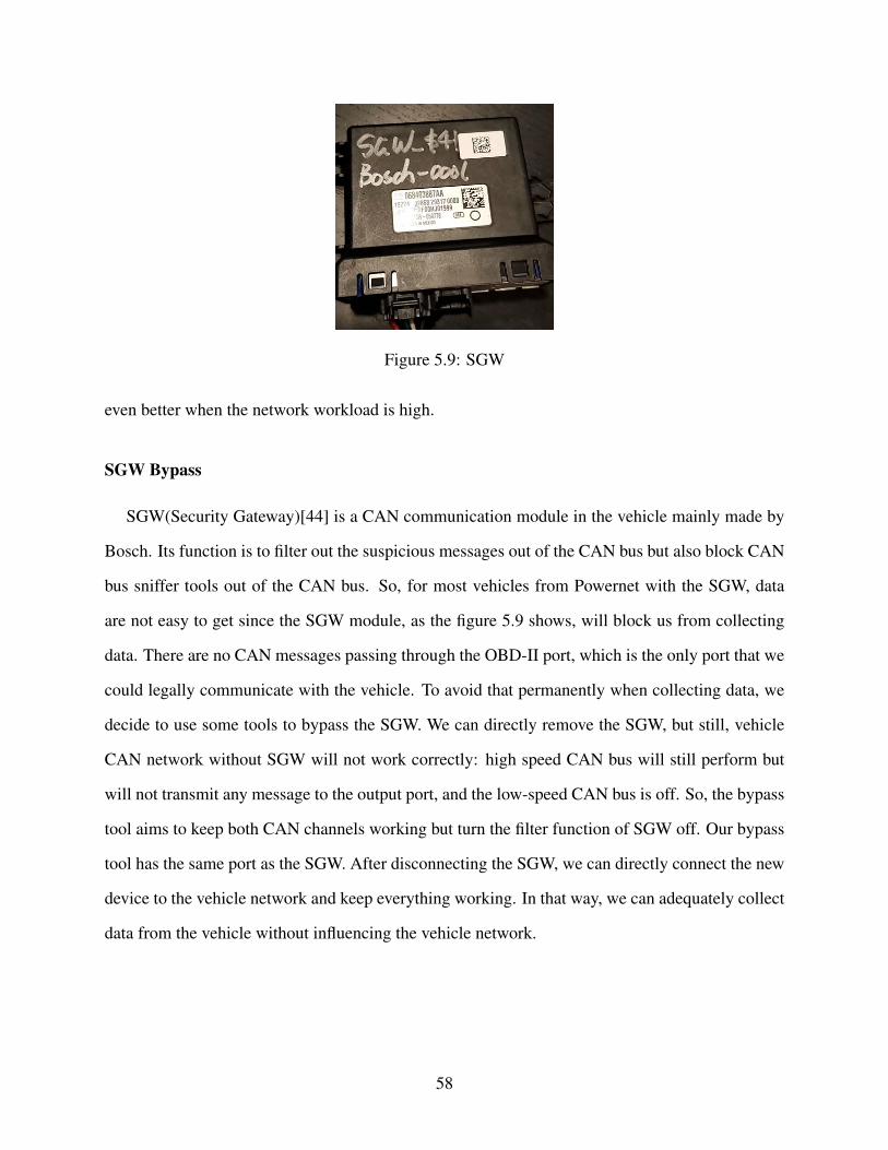
Figure 5.9: SGW

even better when the network workload is high.

SGW Bypass

SGW(Security Gateway)[44] is a CAN communication module in the vehicle mainly made by

Bosch. Its function is to filter out the suspicious messages out of the CAN bus but also block CAN

bus sniffer tools out of the CAN bus. So, for most vehicles from Powernet with the SGW, data

are not easy to get since the SGW module, as the figure 5.9 shows, will block us from collecting

data. There are no CAN messages passing through the OBD-II port, which is the only port that we

could legally communicate with the vehicle. To avoid that permanently when collecting data, we

decide to use some tools to bypass the SGW. We can directly remove the SGW, but still, vehicle

CAN network without SGW will not work correctly: high speed CAN bus will still perform but

will not transmit any message to the output port, and the low-speed CAN bus is off. So, the bypass

tool aims to keep both CAN channels working but turn the filter function of SGW off. Our bypass

tool has the same port as the SGW. After disconnecting the SGW, we can directly connect the new

device to the vehicle network and keep everything working. In that way, we can adequately collect

data from the vehicle without influencing the vehicle network.

58

Test Vehicle

Our test vehicles are mainly from FCA (now called Stellantis) under the Powernet platform.

As mentioned before, the Powernet platform is the most widely used platform among all FCA

vehicles. So, using cars and trucks from Powernet could reflect the state of the art vehicles. The

table 5.4 could tell the vehicles information we are using right now which includes over 12 vehicles

contain all types.

Year Make Model Trim Type2014 Fiat 500 L SUV2020 Chrysler Pacifica [45] Pinnacle Minivan2018 Chrysler Pacifica L Minivan2020 Ram 3500 Laramie Longhorn Truck2008 Lexus IS 350 Sedan2020 Dodge Charger sxt Sedan2019 Infiniti QX80 SUV2021 Dodge Durango GT SUV2010 BMW 135 i Coupe2021 Jeep Grand Wagoneer SUV2022 Jeep Compass TrailHawk SUV2011 Nissan Altima SE Sedan

Table 5.4: Vehicles used for data collection

We can get some data from the vehicle CAN bus for some of the vehicles, but the complete

information from the CAN bus is not collectible. As far as we know, BMW [46] started the new

design of the CAN network as early as 2008, and they encrypted the CAN network since 2009. And

the same situation remains in Infiniti QX80. Although we collect some data from those encrypted

vehicles, the mapper algorithm did not process those data. Still, our primary processed data are

from FCA vehicles, mainly including Dodge SUV figure 5.10, Ram truck figure 5.11, Chrysler

minivan figure 5.8 and a Toyota Sedan.

5.3 Summary

Here is the table 5.5 of all the data we collected. Each dataset should have a period of 15 to

20 minutes under different conditions. Although we collected data from multiple situations, we

59

Figure 5.10: Test vehicle 2021 Dodge Durango GT

only process data while the vehicle is neutral or the vehicle is in switch-on condition. In those

two conditions, the vehicle is in a relatively stable network environment. Every data follows the

format of data collected by the ZLG Canalyst, so there will be several data converters specific to

each dataset.

From the table 5.5, the total size of all kinds of data is over 5GB, except for data we did not

use for the algorithm. The amount of collected data files is 138, containing at least 46 hours of

data collecting time. Based on the size and the number of the data, we can get a relatively reliable

conclusion about our mapper algorithm.

60

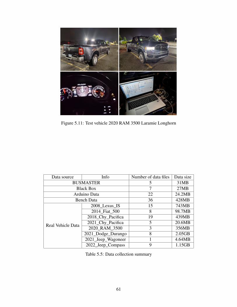
Figure 5.11: Test vehicle 2020 RAM 3500 Laramie Longhorn

Data source Info Number of data files Data sizeBUSMASTER 5 31MB

Black Box 7 27MBArduino Data 22 24.2MBBench Data 36 428MB

Real Vehicle Data

2008_Lexus_IS 15 743MB2014_Fiat_500 8 98.7MB

2018_Chy_Pacifica 19 439MB2021_Chy_Pacifica 5 20.6MB2020_RAM_3500 3 356MB

2021_Dodge_Durango 8 2.05GB2021_Jeep_Wagoneer 1 4.64MB2022_Jeep_Compass 9 1.15GB

Table 5.5: Data collection summary

61

Chapter 6

Vehicle Information Database

It is essential to have a reliable ground truth when verifying the mapper result. Since our

data sources from actual vehicles are mainly from the Powernet platform constructed by FCA,

most of our data files follow similar CAN messages ID and data information. However, they

may use electric modules made by different suppliers. And for vehicles we collect data from,

they may have up to 50 modules contained in the vehicle network and up to nearly 400 message

IDs transmitted on the CAN bus. Building an algorithm to process the data from vehicle ECU

messages automatically is urgent for massive data processing. Besides the need for an automatic

processing algorithm, data collected from different vehicles but the same platforms have multiple

data intersections. Building a database could perfectly solve the problem and make our future

work more straightforward. Then, we create the Vehicle Information Database to store the CAN

bus information about messages information and vehicle information. We build the database using

the Microsoft Postgre platform and keep it in the Google Cloud server that could be loaded using

C++.

6.1 Database Platform

To insert, update and load data from anywhere, we use the Google Cloud SQL server to store

our data. Our database is built based on PostgreSQL 10 and PostgreSQL 13, and pgAdmin4

as our management tools. Google Cloud server could be loaded directly by the pgAdmin4 for

management purposes and by C++ for data processing and application on algorithm purposes.

62

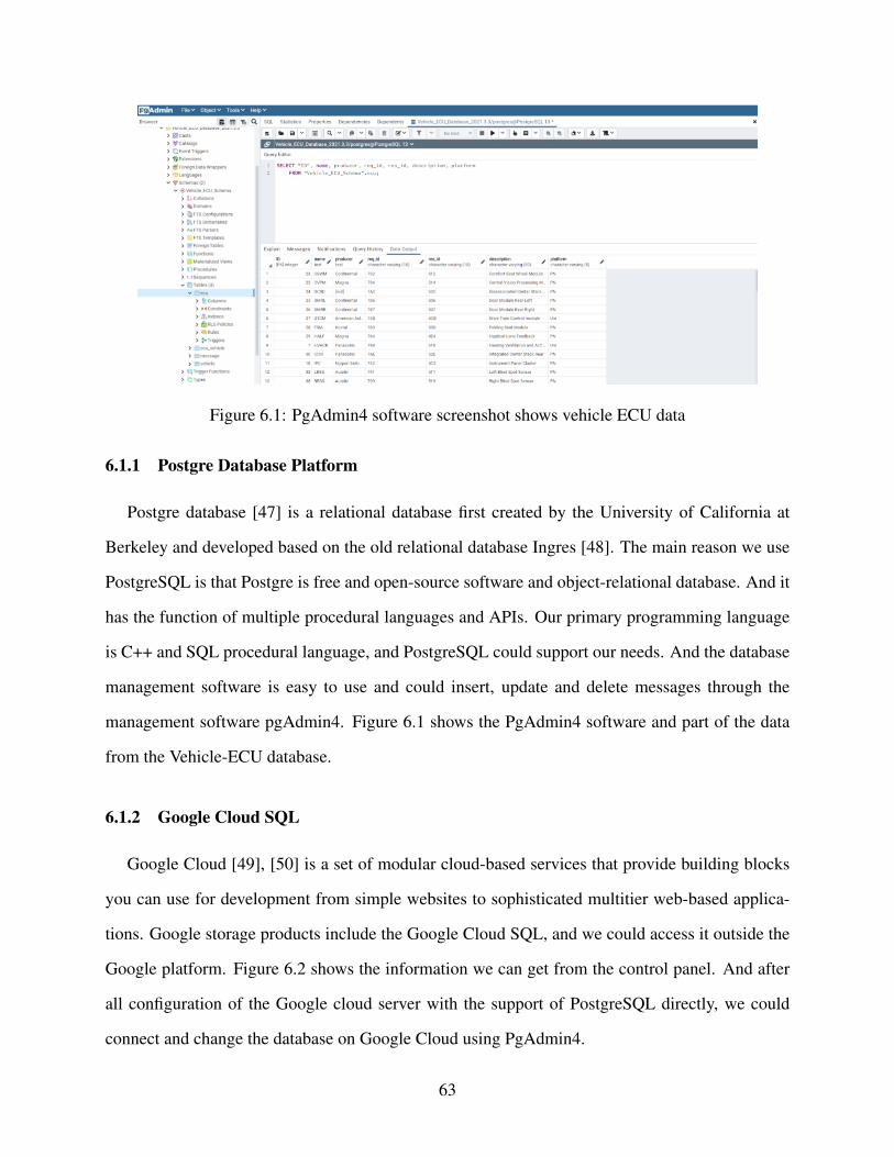
Figure 6.1: PgAdmin4 software screenshot shows vehicle ECU data

6.1.1 Postgre Database Platform

Postgre database [47] is a relational database first created by the University of California at

Berkeley and developed based on the old relational database Ingres [48]. The main reason we use

PostgreSQL is that Postgre is free and open-source software and object-relational database. And it

has the function of multiple procedural languages and APIs. Our primary programming language

is C++ and SQL procedural language, and PostgreSQL could support our needs. And the database

management software is easy to use and could insert, update and delete messages through the

management software pgAdmin4. Figure 6.1 shows the PgAdmin4 software and part of the data

from the Vehicle-ECU database.

6.1.2 Google Cloud SQL

Google Cloud [49], [50] is a set of modular cloud-based services that provide building blocks

you can use for development from simple websites to sophisticated multitier web-based applica-

tions. Google storage products include the Google Cloud SQL, and we could access it outside the

Google platform. Figure 6.2 shows the information we can get from the control panel. And after

all configuration of the Google cloud server with the support of PostgreSQL directly, we could

connect and change the database on Google Cloud using PgAdmin4.

63

Figure 6.2: Google Cloud

6.2 Database Design

The database must meet the information from vehicle and vehicle ECUs we need for the ground

truth ECU. And at the same time, it must keep the efficiency of the database itself and data process-

ing algorithm. All the requirements for the mapper algorithm should include vehicle information,

control module information, and message information. We use essential and unique information

like VIN (vehicle identification number) to connect different data tables. After that, we should

use multiple SQL scripts to help insert, update and delete information in the database. We aim to

improve the efficiency of processing data when executing the mapper algorithm based on the C++

language.

6.2.1 Requirement Analysis

To realize the function we need for our algorithm, we need at least three different tables: vehicle

information table, electronic control module table, and CAN message information table. And we

should connect those three tables. For CAN message database and ECU database, we can realize

the connection using the generated identification number for all ECUs. But to connect the vehicle

information database and the ECU database, we need to create another table to do that job. There

64

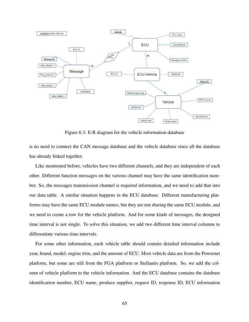
Figure 6.3: E-R diagram for the vehicle information database

is no need to connect the CAN message database and the vehicle database since all the database

has already linked together.

Like mentioned before, vehicles have two different channels, and they are independent of each

other. Different function messages on the various channel may have the same identification num-

ber. So, the messages transmission channel is required information, and we need to add that into

our data table. A similar situation happens in the ECU database. Different manufacturing plat-

forms may have the same ECU module names, but they are not sharing the same ECU module, and

we need to create a row for the vehicle platform. And for some kinds of messages, the designed

time interval is not single. To solve this situation, we add two different time interval columns to

differentiate various time intervals.

For some other information, each vehicle table should contain detailed information include

year, brand, model, engine trim, and the amount of ECU. Most vehicle data are from the Powernet

platform, but some are still from the FGA platform or Stellantis platform. So, we add the col-

umn of vehicle platform to the vehicle information. And the ECU database contains the database

identification number, ECU name, produce supplier, request ID, response ID, ECU information

65

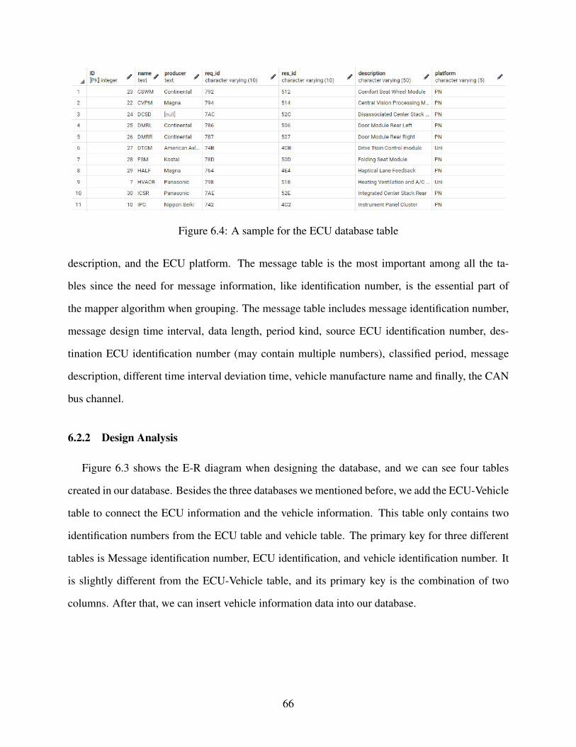
Figure 6.4: A sample for the ECU database table

description, and the ECU platform. The message table is the most important among all the ta-

bles since the need for message information, like identification number, is the essential part of

the mapper algorithm when grouping. The message table includes message identification number,

message design time interval, data length, period kind, source ECU identification number, des-

tination ECU identification number (may contain multiple numbers), classified period, message

description, different time interval deviation time, vehicle manufacture name and finally, the CAN

bus channel.

6.2.2 Design Analysis

Figure 6.3 shows the E-R diagram when designing the database, and we can see four tables

created in our database. Besides the three databases we mentioned before, we add the ECU-Vehicle

table to connect the ECU information and the vehicle information. This table only contains two

identification numbers from the ECU table and vehicle table. The primary key for three different

tables is Message identification number, ECU identification, and vehicle identification number. It

is slightly different from the ECU-Vehicle table, and its primary key is the combination of two

columns. After that, we can insert vehicle information data into our database.

66

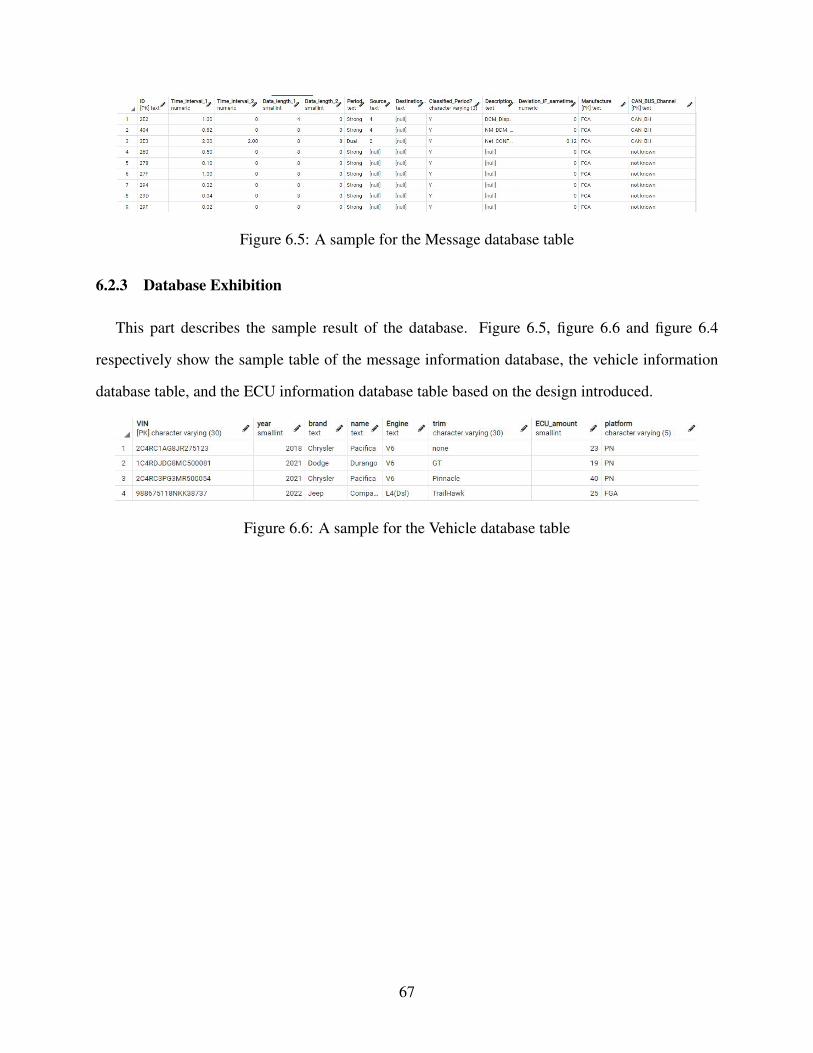
Figure 6.5: A sample for the Message database table

6.2.3 Database Exhibition

This part describes the sample result of the database. Figure 6.5, figure 6.6 and figure 6.4

respectively show the sample table of the message information database, the vehicle information

database table, and the ECU information database table based on the design introduced.

Figure 6.6: A sample for the Vehicle database table

67

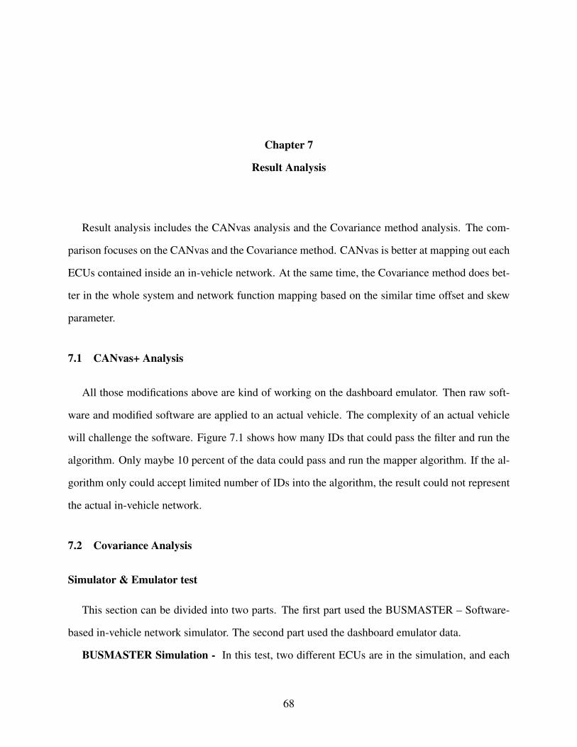
Chapter 7

Result Analysis

Result analysis includes the CANvas analysis and the Covariance method analysis. The com-

parison focuses on the CANvas and the Covariance method. CANvas is better at mapping out each

ECUs contained inside an in-vehicle network. At the same time, the Covariance method does bet-

ter in the whole system and network function mapping based on the similar time offset and skew

parameter.

7.1 CANvas+ Analysis

All those modifications above are kind of working on the dashboard emulator. Then raw soft-

ware and modified software are applied to an actual vehicle. The complexity of an actual vehicle

will challenge the software. Figure 7.1 shows how many IDs that could pass the filter and run the

algorithm. Only maybe 10 percent of the data could pass and run the mapper algorithm. If the al-

gorithm only could accept limited number of IDs into the algorithm, the result could not represent

the actual in-vehicle network.

7.2 Covariance Analysis

Simulator & Emulator test

This section can be divided into two parts. The first part used the BUSMASTER – Software-

based in-vehicle network simulator. The second part used the dashboard emulator data.

BUSMASTER Simulation - In this test, two different ECUs are in the simulation, and each

68

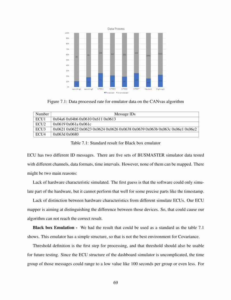
Figure 7.1: Data processed rate for emulator data on the CANvas algorithm

Number Message IDsECU1 0x04a6 0x04b6 0x0610 0x611 0x0613ECU2 0x0619 0x061a 0x061cECU3 0x0621 0x0622 0x0623 0x0624 0x0626 0x0638 0x0639 0x063b 0x063c 0x06e1 0x06e2ECU4 0x063d 0x0680

Table 7.1: Standard result for Black box emulator

ECU has two different ID messages. There are five sets of BUSMASTER simulator data tested

with different channels, data formats, time intervals. However, none of them can be mapped. There

might be two main reasons:

Lack of hardware characteristic simulated. The first guess is that the software could only simu-

late part of the hardware, but it cannot perform that well for some precise parts like the timestamp.

Lack of distinction between hardware characteristics from different simulate ECUs. Our ECU

mapper is aiming at distinguishing the difference between those devices. So, that could cause our

algorithm can not reach the correct result.

Black box Emulation - We had the result that could be used as a standard as the table 7.1

shows. This emulator has a simple structure, so that is not the best environment for Covariance.

Threshold definition is the first step for processing, and that threshold should also be usable

for future testing. Since the ECU structure of the dashboard simulator is uncomplicated, the time

group of those messages could range to a low value like 100 seconds per group or even less. For

69

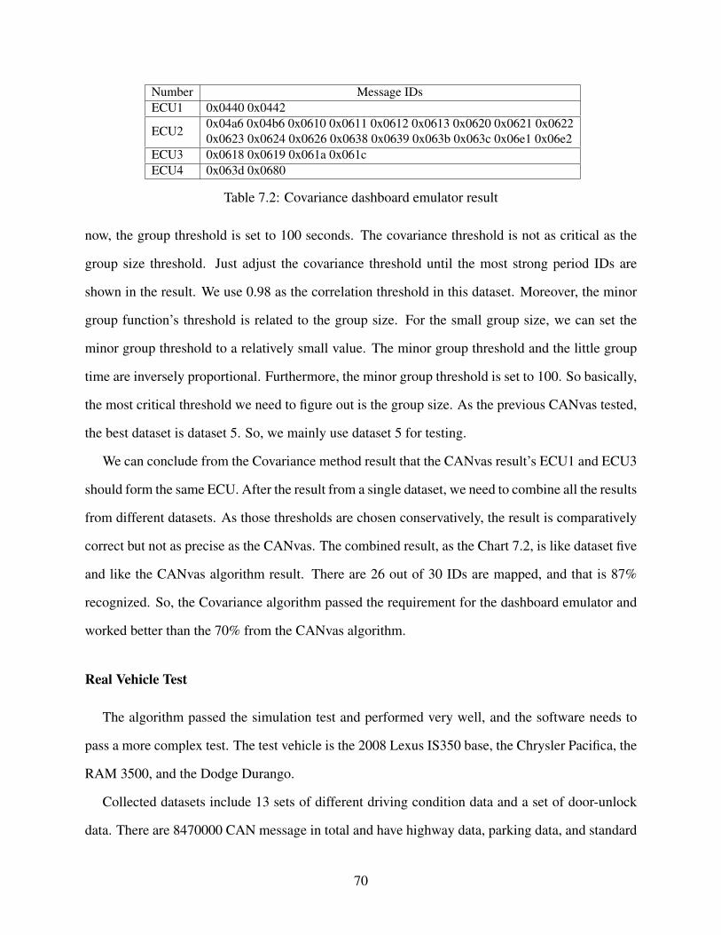
Number Message IDsECU1 0x0440 0x0442

ECU20x04a6 0x04b6 0x0610 0x0611 0x0612 0x0613 0x0620 0x0621 0x06220x0623 0x0624 0x0626 0x0638 0x0639 0x063b 0x063c 0x06e1 0x06e2

ECU3 0x0618 0x0619 0x061a 0x061cECU4 0x063d 0x0680

Table 7.2: Covariance dashboard emulator result

now, the group threshold is set to 100 seconds. The covariance threshold is not as critical as the

group size threshold. Just adjust the covariance threshold until the most strong period IDs are

shown in the result. We use 0.98 as the correlation threshold in this dataset. Moreover, the minor

group function’s threshold is related to the group size. For the small group size, we can set the

minor group threshold to a relatively small value. The minor group threshold and the little group

time are inversely proportional. Furthermore, the minor group threshold is set to 100. So basically,

the most critical threshold we need to figure out is the group size. As the previous CANvas tested,

the best dataset is dataset 5. So, we mainly use dataset 5 for testing.

We can conclude from the Covariance method result that the CANvas result’s ECU1 and ECU3

should form the same ECU. After the result from a single dataset, we need to combine all the results

from different datasets. As those thresholds are chosen conservatively, the result is comparatively

correct but not as precise as the CANvas. The combined result, as the Chart 7.2, is like dataset five

and like the CANvas algorithm result. There are 26 out of 30 IDs are mapped, and that is 87%

recognized. So, the Covariance algorithm passed the requirement for the dashboard emulator and

worked better than the 70% from the CANvas algorithm.

Real Vehicle Test

The algorithm passed the simulation test and performed very well, and the software needs to

pass a more complex test. The test vehicle is the 2008 Lexus IS350 base, the Chrysler Pacifica, the

RAM 3500, and the Dodge Durango.

Collected datasets include 13 sets of different driving condition data and a set of door-unlock

data. There are 8470000 CAN message in total and have highway data, parking data, and standard

70

drive data. When adjusting the Covariance mapper, the parking data is preferred because this kind

of data is stable and easy to get a reliable result. So, we have six sets of data, and that contains two

sets of data that the vehicle engine is not start. If the vehicle is parking with the engine running,

there are 80 messages in the CAN bus. Vehicles at different driving conditions or different modes

may cause the message IDs vary.

The group size threshold and the Covariance threshold need to be adjusted more detail. Each

dataset has 20 minutes of CAN bus data. A more unstable result will be obtained using a low

group size threshold compared to the standard threshold. The standard threshold determined by

The group threshold we are using is 20, and the result is relatively good, as the figure 7.4 shows.

The data might be divided into several different groups, but they are from the same group. If one ID

is altered from one group to another and it’s not stable at all, the primary purpose is to be from the

same ECU. The covariance algorithm needs a good amount of data to depict the mapping result.

If the amount of data is insufficient, all messages will be grouped and cannot separate properly.

That’s short for this algorithm. Obviously, as the figure 7.2 shows, the number of messages in the

result is far more than the CANvas algorithm.

Notice that when the group size is small, the number of ECUs reaches the peak is sooner. If

the data size is limited to a low value and cannot be modified, the group threshold needs to be

relatively lowered to get more ECU results. But at the same time, the group threshold should be

large to eliminate the vibration of the data. Every time we have 40 minutes of data with a large

group size of 30, we can get a stable mapper result. Also, the threshold we are using is 6. The group

size is 30 so that every message that contains time intervals absolute value under five milliseconds

will be grouped. That makes the minor group be the largest in our mapping result. And in the

future, the algorithm on the little group should be optimized.

Figure 7.3 is the combined result from the CANvas algorithm, and figure 7.4 is the combined

result of the Covariance algorithm. Those groups recognized by the CANvas algorithm are from

the same group conducted by the covariance algorithm. It can prove that the algorithm works well,

and it may lead to the complete mapping result of those messages from an actual vehicle.

71

Figure 7.2: Number of data grouped by CANvas algorithm and Covariance algorithm

Figure 7.3: CANvas algorithm result

Advantage and disadvantage over CANvas

There is some comparison with the CANvas while analyzing the Covariance method. This

part compares the CANvas and the Covariance using the bench data and vehicle data collected

from Chrysler Pacifica, RAM 3500, and Dodge Durango. And we will state the advantage of the

Covariance over the CANvas based on those real world condition data.

In an actual vehicle network, especially with a high workload on the vehicle, like the car is driv-

ing or at the neutral condition, the Covariance algorithm will perform better. That is because the

Covariance method could group the vehicle network characteristics rather than the exact hardware

characteristic of each ECU module. Although ECU modules should have similar hardware charac-

teristics, some ECU modules may take multiple responsibilities with multiple hardware mounted,

like gateway module. Those ECU modules are hard to determine the hardware characteristic,

72

Figure 7.4: Covariance algorithm result

Vehicle Name GT ECU GR ECU from the CANvas GR ECU from Covariance2018 Pacifica 14 6 102021 Pacifica 12 6 122020 RAM 3500 19 11 132021 Dodge Durango GT 19 11 16

Table 7.3: Comparison between CANvas(LCM) and Covariance on number of the ECU

which is why the network and hardware characteristics based Covariance method could work bet-

ter. Table 7.3 shows the Covariance method has more advantage in the number of ECUs contained

in the network compared with the CANvas.

Overall, for a simple vehicle network environment with a low workload on the CAN bus, the

CANvas tool using the CANvas performs better than the Covariance. But for CAN networks with

high workloads, like current modern vehicles with 40 or more modules mounted on the CAN

bus, the Covariance grouping method works better than the CANvas. The difference between the

two algorithms is that the CANvas tool with the CANvas aims to map precisely the messages

corresponding with the modules. But the Covariance tool utilizes the network block that may

contain messages from different ECUs. The number of operations has in the vehicle network

should be similar to the number of modules mounted on the CAN bus. So, finally, we can also

reach the point of mapping out the whole vehicle network. That comes to the end of algorithm

improvement and the result analysis of the thesis.

73

Chapter 8

Conclusion and Future Work

8.1 Conclusion

In this thesis, we introduce our design and implement of a novel CAN mapper system. Com-

pared with existing CAN mappers which suffer from their hardware characteristic-based algo-

rithms, our mapper improves mapping accuracy in complicated network environment by using

correlation information among CAN message timestamps that implies not just hardware character-

istics but also network function characteristics of source ECU. We implement Covariance and test

it over data collected from the Arduino emulator, dashboard emulator, manufacturing development

bench, and testing vehicles by six data logging tools. Our new Covariance mapper tool could reach

an average of 77.8% accuracy based on our testing results compared with an average of 51.9%

of existing mappers. In addition to mapper algorithm design and development, this thesis also

contributes to the setup of ECU information database, including message information and vehicle

information affiliated, from some current Stellantis model vehicles.

8.2 Future Work

The performance and applicability of our system can be further improved by advancing the

following directions:

Processing discontinuous messages

As mentioned above, the messages collected from CAN bus can be divided into three cate-

gories: strong period, discontinuous and unclassified. Our system only uses strong period data for

74

processing. As a future work direction, we can add discontinuous data to the mapper algorithm.

Discontinuous data is strong period data with several significant gaps in the time intervals when

sending. Such gaps can reflect the characteristic of the senders. To make use of such discontinuous

messages, our system needs to find a way to connect them.

Applying Machine Learning-based Algorithm

Other than the two main algorithms we mentioned in the thesis, we also tested the machine

learning clustering algorithm. We found that the machine learning algorithm could provide satis-

factory performance in certain experimental settings. As a future direction, we will further explore

machine learning algorithms’ usages in mapping.

Improving Threshold Decision

Our algorithm relies on finding the optimal threshold values for group size and correlation. Our

current threshold decision methodology is to calculate such thresholds by data extracted from test

vehicles. To improve the optimally of such thresholds on new coming vehicles, another future work

direction is to generate these threshold in an adaptive way. The threshold is mainly influenced by

the speed of data transmitted on the CAN bus, the workload of the CAN bus, the total amount of

data contained in the vehicle, and the structure design of the vehicle. One possible solution is to

study the correlation between the optimal thresholds and the vehicle network conditions.

Collecting More Data from Different Contexts

The system is built and tested upon data collected from vehicles at a few selected statuses

(ignition on status, engine running status, and driving status). To further improve our system’s per-

formance in wider usage scenarios, more data can be collected from other vehicle status contexts

(e.g., driving in heavy rain), where more ECU modules are transmitting data and the CAN traffic

workload is heavier.

75

References

[1] S. C. HPL, “Introduction to the controller area network (can),” Application Report SLOA101,pp. 1–17, 2002.

[2] G. F. Lyon, Nmap network scanning: The official Nmap project guide to network discoveryand security scanning. Insecure. Com LLC (US), 2008.

[3] I. Rouf, R. D. Miller, H. A. Mustafa, T. Taylor, S. Oh, W. Xu, M. Gruteser, W. Trappe, andI. Seskar, “Security and privacy vulnerabilities of in-car wireless networks: A tire pressuremonitoring system case study.,” in USENIX Security Symposium, vol. 10, 2010.

[4] E. Hallett, R. Woodward, S. Schultz, and R. Vaidyanathan, “Rapid bicycle gear switchingbased on physiological cues,” in 2015 IEEE International Conference on Automation Sci-ence and Engineering (CASE), IEEE, 2015, pp. 377–382.

[5] J. Norden, M. O’Kelly, and A. Sinha, “Efficient black-box assessment of autonomous vehi-cle safety,” arXiv preprint arXiv:1912.03618, 2019.

[6] H.-J. Liao, C.-H. R. Lin, Y.-C. Lin, and K.-Y. Tung, “Intrusion detection system: A compre-hensive review,” Journal of Network and Computer Applications, vol. 36, no. 1, pp. 16–24,2013.

[7] M. Aloqaily, S. Otoum, I. Al Ridhawi, and Y. Jararweh, “An intrusion detection system forconnected vehicles in smart cities,” Ad Hoc Networks, vol. 90, p. 101 842, 2019.

[8] H. M. Song, H. R. Kim, and H. K. Kim, “Intrusion detection system based on the analysisof time intervals of can messages for in-vehicle network,” in 2016 international conferenceon information networking (ICOIN), IEEE, 2016, pp. 63–68.

[9] K. Kim, J. S. Kim, S. Jeong, J.-H. Park, and H. K. Kim, “Cybersecurity for autonomousvehicles: Review of attacks and defense,” Computers & Security, p. 102 150, 2021.

[10] S. Kulandaivel, T. Goyal, A. K. Agrawal, and V. Sekar, “Canvas: Fast and inexpensive au-tomotive network mapping,” in 28th {USENIX} Security Symposium ({USENIX} Security19), 2019, pp. 389–405.

[11] L. Zhang, L. Shi, N. Kaja, and D. Ma, “A two-stage deep learning approach for can intrusiondetection,” in Proc. Ground Vehicle Syst. Eng. Technol. Symp.(GVSETS), 2018, pp. 1–11.

[12] H. Ueda, R. Kurachi, H. Takada, T. Mizutani, M. Inoue, and S. Horihata, “Security authen-tication system for in-vehicle network,” SEI technical review, vol. 81, pp. 5–9, 2015.

[13] T. H. Pearl, “Fast & furious: The misregulation of driverless cars,” NYU Ann. Surv. Am. L.,vol. 73, p. 19, 2017.

[14] J. Claybrook and S. Kildare, “Autonomous vehicles: No driver. . . no regulation?” Science,vol. 361, no. 6397, pp. 36–37, 2018.

76

[15] I. Yaqoob, L. U. Khan, S. M. A. Kazmi, M. Imran, N. Guizani, and C. S. Hong, “Au-tonomous driving cars in smart cities: Recent advances, requirements, and challenges,” IEEENetwork, vol. 34, no. 1, pp. 174–181, 2020. DOI: 10.1109/MNET.2019.1900120.

[16] V. A. Banks, K. L. Plant, and N. A. Stanton, “Driver error or designer error: Using theperceptual cycle model to explore the circumstances surrounding the fatal tesla crash on 7thmay 2016,” Safety science, vol. 108, pp. 278–285, 2018.

[17] A. Ceder and N. H. Wilson, “Bus network design,” Transportation Research Part B: Method-ological, vol. 20, no. 4, pp. 331–344, 1986.

[18] G. Cena and A. Valenzano, “An improved can fieldbus for industrial applications,” IEEEtransactions on industrial electronics, vol. 44, no. 4, pp. 553–564, 1997.

[19] R. Li, C. Liu, and F. Luo, “A design for automotive can bus monitoring system,” in 2008IEEE vehicle power and propulsion conference, IEEE, 2008, pp. 1–5.

[20] H. Hilpert, L. Thoroe, and M. Schumann, “Real-time data collection for product carbonfootprints in transportation processes based on obd2 and smartphones,” in 2011 44th HawaiiInternational Conference on System Sciences, 2011, pp. 1–10. DOI: 10.1109/HICSS.2011.356.

[21] L. Ran, W. Junfeng, W. Haiying, and L. Gechen, “Design method of can bus network com-munication structure for electric vehicle,” in International Forum on Strategic Technology2010, IEEE, 2010, pp. 326–329.

[22] B. Groza, H.-E. Gurban, and P.-S. Murvay, “Designing security for in-vehicle networks:A body control module (bcm) centered viewpoint,” in 2016 46th Annual IEEE/IFIP In-ternational Conference on Dependable Systems and Networks Workshop (DSN-W), 2016,pp. 176–183. DOI: 10.1109/DSN-W.2016.26.

[23] A. Sawant, S. Lenina, and M. D. Joshi, “Can, flexray, most versus ethernet for vehicularnetworks,” Int. J. Innov. Adv. Comput. Sci. IJIACS, vol. 7, no. 4, 2018.

[24] R. Makowitz and C. Temple, “Flexray-a communication network for automotive controlsystems,” in 2006 IEEE International Workshop on Factory Communication Systems, IEEE,2006, pp. 207–212.

[25] S. Woo, H. J. Jo, I. S. Kim, and D. H. Lee, “A practical security architecture for in-vehiclecan-fd,” IEEE Transactions on Intelligent Transportation Systems, vol. 17, no. 8, pp. 2248–2261, 2016.

[26] P. Hank, S. Müller, O. Vermesan, and J. Van Den Keybus, “Automotive ethernet: In-vehiclenetworking and smart mobility,” in 2013 Design, Automation & Test in Europe Conference& Exhibition (DATE), IEEE, 2013, pp. 1735–1739.

[27] Y. Xu, J. Wang, W. Chen, J. Tao, and Q. Liu, “Application of lin bus in vehicle network,”in 2006 IEEE International Conference on Vehicular Electronics and Safety, IEEE, 2006,pp. 119–123.

[28] J. H. Kim, S.-H. Seo, N.-T. Hai, B. M. Cheon, Y. S. Lee, and J. W. Jeon, “Gateway frame-work for in-vehicle networks based on can, flexray, and ethernet,” IEEE Transactions onVehicular Technology, vol. 64, no. 10, pp. 4472–4486, 2015. DOI: 10.1109/TVT.2014.2371470.

77

[29] B. Groza, S. Murvay, A. Van Herrewege, and I. Verbauwhede, “Libra-can: A lightweightbroadcast authentication protocol for controller area networks,” in International Conferenceon Cryptology and Network Security, Springer, 2012, pp. 185–200.

[30] H. Schweppe, Y. Roudier, B. Weyl, L. Apvrille, and D. Scheuermann, “Car2x communi-cation: Securing the last meter-a cost-effective approach for ensuring trust in car2x ap-plications using in-vehicle symmetric cryptography,” in 2011 IEEE Vehicular TechnologyConference (VTC Fall), IEEE, 2011, pp. 1–5.

[31] C. Szilagyi and P. Koopman, “Low cost multicast authentication via validity voting in time-triggered embedded control networks,” in Proceedings of the 5th Workshop on EmbeddedSystems Security, 2010, pp. 1–10.

[32] P. Gasti, G. Tsudik, E. Uzun, and L. Zhang, “Dos and ddos in named data networking,” in2013 22nd International Conference on Computer Communication and Networks (ICCCN),IEEE, 2013, pp. 1–7.

[33] M.-L. Zhang and Z.-H. Zhou, “Ml-knn: A lazy learning approach to multi-label learning,”Pattern recognition, vol. 40, no. 7, pp. 2038–2048, 2007.

[34] G. Guo, H. Wang, D. Bell, Y. Bi, and K. Greer, “Knn model-based approach in classifica-tion,” in OTM Confederated International Conferences" On the Move to Meaningful InternetSystems", Springer, 2003, pp. 986–996.

[35] E. Schubert, J. Sander, M. Ester, H. P. Kriegel, and X. Xu, “Dbscan revisited, revisited: Whyand how you should (still) use dbscan,” ACM Transactions on Database Systems (TODS),vol. 42, no. 3, pp. 1–21, 2017.

[36] D. Birant and A. Kut, “St-dbscan: An algorithm for clustering spatial–temporal data,” Data& knowledge engineering, vol. 60, no. 1, pp. 208–221, 2007.

[37] A. Tahat, A. Said, F. Jaouni, and W. Qadamani, “Android-based universal vehicle diagnosticand tracking system,” in 2012 IEEE 16th International Symposium on Consumer Electron-ics, IEEE, 2012, pp. 137–143.

[38] S. K. Pitla, J. D. Luck, J. Werner, N. Lin, and S. A. Shearer, “In-field fuel use and loadstates of agricultural field machinery,” Computers and Electronics in Agriculture, vol. 121,pp. 290–300, 2016.

[39] S. E. Marx, J. D. Luck, S. K. Pitla, and R. M. Hoy, “Comparing various hardware/softwaresolutions and conversion methods for controller area network (can) bus data collection,”Computers and Electronics in Agriculture, vol. 128, pp. 141–148, 2016.

[40] H. Kashif, G. Bahig, and S. Hammad, “Can bus analyzer and emulator,” in 2009 4th Inter-national Design and Test Workshop (IDT), IEEE, 2009, pp. 1–4.

[41] Z. Ling, “The design for can bus based on arduino system,” Computer Programming Skills& Maintenance, vol. 2012, p. 20, 2012.

[42] A. S. Siddiqui, Y. Gui, J. Plusquellic, and F. Saqib, “Secure communication over canbus,”in 2017 IEEE 60th International Midwest Symposium on Circuits and Systems (MWSCAS),IEEE, 2017, pp. 1264–1267.

[43] W. Voss, Controller area network prototyping with Arduino. Lulu Press, Inc, 2015.

78

[44] J. H. Kim, S.-H. Seo, N.-T. Hai, B. M. Cheon, Y. S. Lee, and J. W. Jeon, “Gateway frame-work for in-vehicle networks based on can, flexray, and ethernet,” IEEE Transactions onVehicular Technology, vol. 64, no. 10, pp. 4472–4486, 2014.

[45] D. Zetsche, “Chrysler group–disciplined pizzazz: Leveraging the strengths,” Markenman-agement in der Automobilindustrie: Die Erfolgsstrategien internationaler Top-Manager,p. 203, 2005.

[46] R. Shaw and B. Jackman, “An introduction to flexray as an industrial network,” in 2008IEEE International Symposium on Industrial Electronics, IEEE, 2008, pp. 1849–1854.

[47] B. Momjian, PostgreSQL: introduction and concepts. Addison-Wesley New York, 2001,vol. 192.

[48] G. Held, M. Stonebraker, and E. Wong, “Ingres: A relational data base system,” in Proceed-ings of the May 19-22, 1975, national computer conference and exposition, 1975, pp. 409–416.

[49] N. Saravanan, A. Mahendiran, N. V. Subramanian, and N. Sairam, “An implementationof rsa algorithm in google cloud using cloud sql,” Research Journal of Applied Sciences,Engineering and Technology, vol. 4, no. 19, pp. 3574–3579, 2012.

[50] S. Krishnan and J. L. U. Gonzalez, Building your next big thing with google cloud platform:A guide for developers and enterprise architects. Springer, 2015.

79