A NEW ISOSTATIC MODEL FOR THE EAST PACIFIC RISE CREST

JOURNAL OF GEOPHYSICAL RESEARCH, VOL. 89, NO. B12, PAGES 9997-10,015, NOVEMBER 10, 1984

A NEW ISOSTATIC MODEL FOR THE EAST PACIFIC RISE CREST

John A. Madsen

Graduate School of Oceanography, University of Rhode Island, Kingston

Donald W. Forsyth

Department of Geological Sciences, Brown University, Providence, Rhode Island

Robert S. Detrick

Graduate School of Oceanography, University of Rhode Island, Kingston

Abstract. We have developed a new isostatic model for the East Pacific Rise (EPR) that explains the origin of both the axial topographic high and the rise crest gravity anomaly. Our model involves a thin elastic plate, with a constant thickness crust, that is broken at the ridge crest. We assume that a buoyant force

described as an axial horst by Anderson and Noltimier [1973], more closely resembles a narrow, axial "shield volcano" with a summit rift zone

bounded by marginal horst and graben topography [Lonsdale, 1977]. This crestal ridge rises several hundred meters above the surrounding seafloor. Its width is typically 10-20 km or less

beneath the plate bends the free edge of the plate at its base and less than 2 km near the summit. upward at the rise axis forming the topographic high and the rise crest gravity anomaly. We have used this model, and two conventional isostatic models, to examine the isostasy of three segments of the EPR: at 9ø-14•, 6ø-11øS, and 16ø-21øS. Rather than modeling individual profiles we have stacked (summed) the gravity and bathymetry data in each area and computed a single, 200-km-long, mean, mirrored profile for each different ridge segment. These stacked profiles are a remarkable improvement over even the best individual profiles and clearly show both the axial topographic high and its associated free air gravity anomaly. In all three areas the best fitting model parameters are similar and give average compensation depths of about 6-7 km below the seafloor (near the base of the oceanic crust) and an upper limit on the

It is remarkably continuous and linear over considerable distances along-strike and is apparently a steady state feature of intermediate- and fast-spreading ridges [Lonsdale, 1977; CYAMEX Scientific Team and Pastouret, 1981]. The positive free air gravity anomaly associated with this central high is typically small in amplitude (10-20 mGal), about 20-40 km wide, and usually flanked by smaller-amplitude gravity lows [Cochran, 1979].

Several models have been proposed for the origin of the axial topographic high and the rise crest gravity anomaly. Anderson and Noltimier [1973], extending a model of Deffeyes [1970], argued that axial highs are steady state features of ridges spreading fast enough that new material is intruded over a narrower zone than that

flexural rigidity of the plate that increases from required to accelerate the new crust to its full about 1018 N m at the ridge axis to about 3x1019 N spreading velocity. Although this model does not m 5 km from the axis and 1020 N m 25 km or more from the rise crest. These results indicate that

the EPR crest is compensated at much shallower depths than suggested by previous investigators. Our results are consistent with the presence of a small, low-density magma chamber in the lower crust, although at least part of the compensating

explicitly address the mechanism of isostasy, the elevation of the axial high is caused by thicker crust at the ridge axis, presumably providing buoyancy and local (Airy) compensation at the layer 2/layer 3 interface or at the base of the crust. Another model involving local compensation was advocated by Rea [1975], Rosendahl [1976], and

root for the axial high must extend into the upper Sleep and Rosendahl [1979]. In this model the mantle. We interpret the low upper mantle buoyancy needed to elevate the axial region is densities below the rise crest as a zone of provided by an underlying magma chamber. Noting partial melt which accumulates at the base of the geological [e.g., Cann, 1974; Bryan and Moore, oceanic crust between episodic rifting events when 1977; RISE Project Group, 1980] and geophysical the overlying crustal magma chamber is [e.g., Sleep, 1975; Orcutt et al., 1976; Reid et replenished. al., 1977; Herron et al., 1980] evidence for the

presence of a shallow (2-3 km depth) magma chamber Introduction along at least parts of the EPR axis, Sleep and

Rosendahl [1979] assumed that there is a broad, The axes of intermediate and fast-spreading crustal magma chamber underlying the entire axial

mid-ocean ridges, like the East Pacific Rise (EPR) high. Although their complete model includes and the Galapagos spreading center, are characterized by a topographic high or central peak and a shortwavelength, positive free air gravity anomaly. The topographic high, initially

Copyright 1984 by the American Geophysical Union.

Paper number 4B0701. 0148-0227/84/004B-0701505.00

modification of the topography by the strength of the lithosphere, they showed that with reasonable values for the temperature and density of the rise crest they could explain the height of the axial block with local isostatic compensation. Lateral density changes within their model occur primarily within the crust.

Lewis [1982], however, showed that the gravity anomaly associated with the axial high is not

9997

9998 Madsen et al.: Isostatic Model for the East Pacific Rise

consistent with simple Airy compensation by a shallow, low-density magma chamber located entirely within the crust. An Airy model is acceptable but only if the depth of compensation is 10-20 km or more [Cochran, 1979; Lewis, 1982]. Lewis argued that such large compensation depths are physically unreasonable since they preclude the existence of thermally induced density changes above 20 km which are believed to be responsible for both the observed axial topography and heat

density contrast of 0.10-0.25 Mg m -3 is one model that is consistent with the observed data.

Although dynamic support for the axial topography cannot be ruled out, we believe that a satisfactory isostatic model can be constructed.

In this paper we reexamine the isostasy of the EPR by using gravity and topography profiles across three different segments of the rise axis: at 9ø-14øN, 6ø-11øS, and 16ø-21øS. Rather than modeling individual profiles, we have stacked the

flux. Similarly, Lewis [1981] showed that thermal gravity and bathymetry data and computed a single models of the rise crest [Sleep, 1975] with local mean, mirrored profile for each area. We isostasy predict an axial gravity high that is interpret these stacked profiles using much smaller than the observed anomaly, even conventional Airy and elastic plate models as well though these models accurately predict seafloor as a new isostatic model that involves an elastic topography. plate, with a constant thickness crust, that is

Cochran [1979], McNutt [1979], and Lewis [1982] weak at the ridge axis and buoyed up from below. have shown that the topography and gravity This isostatic model is new in the sense that we observed near the axis of the EPR is consistent present, for the first time, an attempt to use a with a regional model of isostasy in which broken plate model in a systematic inversion of topography emplaced on the surface of an elastic topography and gravity data at a spreading center. plate is supported locally by stresses within the Sleep and Rosendahl [1979] previously incorporated plate. Although it is often overlooked, this type a mechanical plate on top of a cooling of model implies that the topography is formed by lithosphere, and Louden and Forsyth [1982] constructional volcanism (as Lonsdale [1977] stressed the importance of loading from below in suggested for at least the central portion of the creating seafloor topography. axial shield volcano) or by some other means of Our results are consistent with the presence of creating topographic relief on top of the plate. a small, low-density magma chamber in the lower The amplitude of the axial free air anomaly crust, although at least part of the compensation [Lewis, 1982] and the admittance function [McNutt, for the axial high must be placed in the upper 1979; Cochran, 1979] appear to require plate thicknesses of the order of 1-6 km if the primary density contrast is at the base of the crust.

There are, however, several physical objections to this model as an explanation for the origin of the axial topographic high. First, if there really is a magma chamber 2-3 km below the seafloor or if existing thermal models are correct, then the effective elastic thickness of the plate is unlikely to be greater than about 2 km at the rise axis. Since the uppermost part of the crust is thought to have little strength, it is unlikely that the plate is strong enough to support the axial topography [Lewis, 1982]. Second, if the plate thickness is small, then the plate model predicts a thickening of the crust toward the rise axis because of the deflection of

the Moho beneath the load of the axial• high [Lewis, 1982]. Multichannel seismic reflection data show no evidence for significant crustal thickening beneath the rise axis [Stoffa et al., 1980]. However, the principal objection is that, in this model the axial high cannot be a steady state feature. Once topography is supported by stresses within the plate, it will be transported laterally away from the rise axis by the moving lithosphere. Thus, if the constructional volcanism that creates the high continues, the axial high will broaden with time until the entire seafloor is shallower and no axial high remains.

mantle near the base of the oceanic crust. These

low upper mantle densities are interpreted as a zone of partial melt in the upper mantle.

Data Sources and Description

Surface ship gravity and bathymetry profiles across three different segments of the EPR were obtained from the National Geophysical and Solar Terrestrial Data Center and Lamont-Doherty

Geological Observatory The three regions 9 o_ o_1 {6o_2 o ' 14•N, 6 løS, and 1 S, were selected for study because there is a large amount of data available in each region and because comparisons of the bathymetry and gravity profiles between these regions allow variations in tectonic processes along the EPR to be investigated.

The data sources and information on

instrumentation and navigation are summarized in Table 1. The overall accuracy of the gravity measurements is dependent on the type of instrumentation and navigation used in the survey. Generally, the accuracy is estimated to be 2-5 mGal for the Gss2 sea gravimeter and the vibrating-string gravimeter when used with satellite navigation. Somewhat larger errors are expected for data collected using a gimbal-mounted gravimeter or celestial navigation.

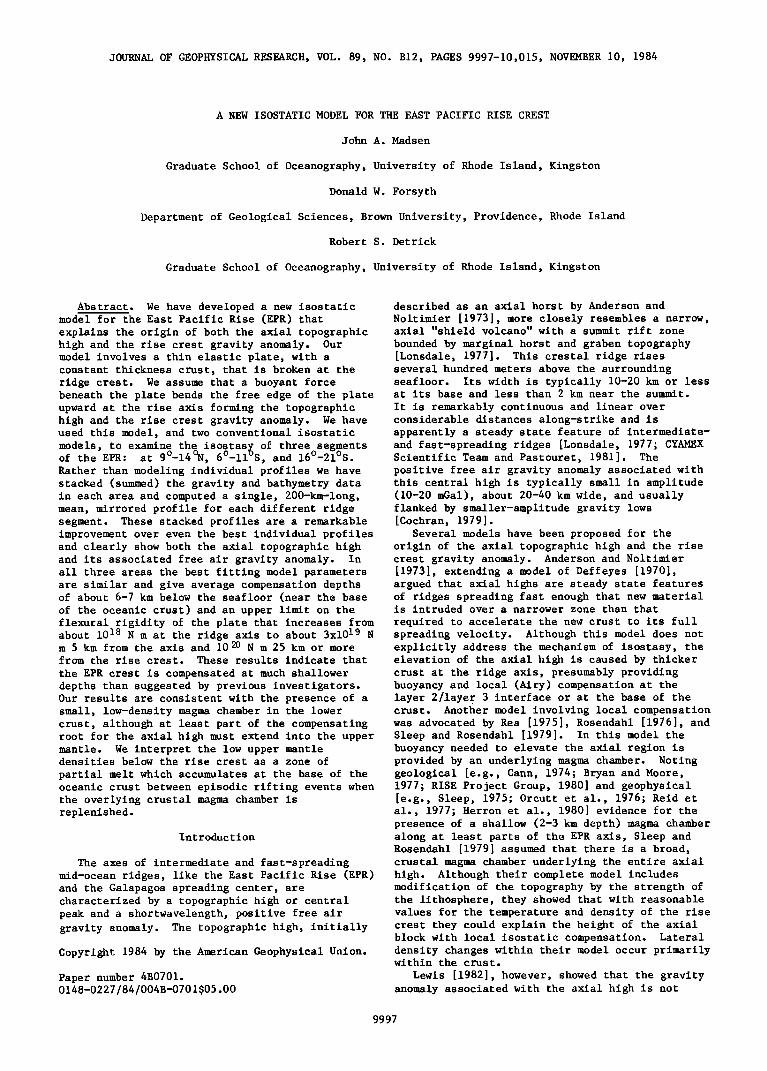
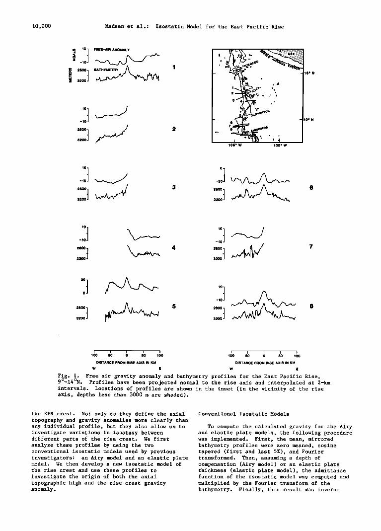
Individual bathymetry and free air gravity profiles were constructed by projecting the

Arguing that neither the Airy nor elastic plate original lines perpendicular to the local strike models provide a satisfactory physical explanation of the ridge and interpola•ting at 2-km intervals. of the topography and gravity at the rise axis, The profiles for the 9ø-14øN area are shown in Lewis [1982, 1983a,b] has suggested that the ridge Figure 1, the 6ø-11øS area in Figure 2, and the crest is dynamically not isostatically supported. 16ø-21øS area in Figure 3. An examination of the He proposes that the positive gravity anomaly at individual bathymetry and gravity profiles in each the rise crest results, in part, from the density region reveals that although they are similar in contrast between the magma chamber and less dense general form, there is considerable variability highly fractured crustal rocks to either side. He from profile to profile. The fact that many of finds that an uncompensated dike-shaped body in these anomalies cannot be correlated between the crust with a width of 2 km and a positive profiles strongly suggests that they are the

Madsen et al.: Isostatic Model for the East Pacific Rise 9999

TABLE 1. Summary of Data Sources

Profile

Cruise and

Ship Year Leg Gr avime t er Stable Platform Navigation

1

2

3,4 5,7 6,8

9-14øN ROBERT D. CONRAD 1966 1011 Graf-Askania Gss2 Anschutz

ROBERT D. CONRAD 1970 1307 Graf-Askania Gss2 Anschutz ROBERT D. CONRAD 1979 2202 Graf-Askania Gss2 Aeroflex

THOMAS WASHINGTON 1976 Deepsonde 2 Graf-Askania Gss2 Anschutz ROBERT D. CONRAD 1976 2002 Graf-Askania Gss2 Aeroflex

6-11øN 1 VEMA 1965 2104

2 , 3 , 4 , 5 , 6 , 8 , 9 OCEANOGRAPHER 1973 4 7 ROBERT D. CONRAD 1967 1111

10 CHAIN 1971 100-11

16-21øS

celestial

satellite

satellite

satellite

satellite

Graf-Askania Gss2 Anschutz celestial

Lacoste-Romberg gimbal mounted satellite Graf-Askania Gss2 Anschutz celestial

VSA Sperry gyrotable satellite

1,3,4,6,7,8,9,10 OCEANOGRAPHER 1973 2 Lacoste-Romberg gimbal mounted satellite 2 VEMA 1963 1905 Graf-Askania Gss2 Alidade celestial

5 OCEANOGRAPHER 1973 3 Lacoste-Romberg gimbal mounted satellite

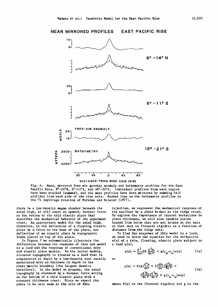
result of local crustal heterogeneity and are not vary in a systematic way between regions. The related to the fundamental structure of the ridge. flanking lows are broad (35 km) and have an In order to minimize this variability and to amplitude of 3-4 mGal at 9ø-14øN, are not present enhance the topographic and gravity signature at 6ø-11øS and are narrow (15 km) with an associated with the rise crest itself, we have amplitude of 3 mGal at 16ø-21øS. These stacked (summed) the bathymetry and gravity data observations suggest that minor variations in the in each area. Stacking was done by summing half isostasy of the crestal region occur along the profiles, each 100 km long, from both sides of the EPR. rise axis. The resulting mean half profiles were then mirrored, eliminating any asymmetries present Isostatic Models in the original data.

The resulting mean, mirrored profiles are shown Two different approaches have previously been in Figure 4 for the 9ø-14øN, 6ø-11øS, and 16ø-21øS used to model the isostasy of the East Pacific regions, respectively. The stacked profiles are a Rise crest. Cochran [1979] used cross-spectral remarkable improvement over even the best techniques to analyze the relationship between individual profiles and clearly show both the gravity and bathymetry on 24 profiles crossing the axial topographic high and the associated free air rise crest between 13øN and 28øS. The cross gravity anomaly. The lack of fit of the /-• spectrum and power spectrum of gravity and depth-age curve [Parsons and Sclater, 1977] to the bathymetry were averaged for all of these profiles topography at the rise crest clearly illustrates and used to calculate a single admittance or that the axial high is not simply a feature response function which was then compared to related to the conductive cooling of the thermal isostatic models based on different compensation lithosphere (the predicted topographic peak at the mechanisms. Since the individual profiles were axis is even less pronounced when a conductive 300 km long, the results reflect the isostasy of cooling model that does not have a singularity in both the crestal region and the ridge flanks; the heat flow at the axis is used [Sleep, 1975]). The compensation of the axial region alone was not free air gravity anomalies are strongly correlated separately investigated. Since a single with the deviations from the depth-age curve. admittance function was determined for all of the

The first-order size and shape of these profiles, along-strike variations in the isostasy anomalies do not appear to vary significantly of the rise crest were averaged out. despite spreading rates that increase by almost Lewis [1982] has directly compared the observed 50% between 14øN (97 mm/y_r full rate [Klitgord and gravity anomalies on three profiles crossing the

9 ø Mammerickx, 1982]) and 21øS (162 mm/yr full rate EPR between N and 12øN with the predicted [Rea, 1978]). There are, however, second-order gravity anomaly calculated assuming different differences in both the rise crest bathymetry and isostatic mechanisms. One advantage of this gravity between the medium fast 9ø-14øN region and approach is that the fit of the data at the rise the fast-spreading 6ø-11øS and 16ø-21øS areas. axis can be directly evaluated. Another potential Both the width and the maximum height of the axial advantage is that the differences between topographic high decrease from 9ø-14øN to individual profiles can be used to investigate

o o 16 -21 S. The width decreases from 20 km at along-strike variations in the isostasy of the 9ø-14øN to 18 km at 6ø-11øS to 15 km at 16ø-21øS, and the maximum height decreases from 400 m at 9ø-14øN to 300 m at 16ø-21øS. The free air anomaly high associated with the rise crest also decreases in width (35-15 km) and amplitude (12-7 mGal) from 9ø-14øN to 16ø-21øS, although the flanking gravity anomaly lows do not appear to

rise crest. Unfortunately, the gravity signal associated with the rise crest is small (~10 mGal), and structural inhomogeneities along individual profiles can mask the fundamental gravity signal associated with the rise crest.

The mean, mirrored profiles we have computed are ideally suited for examining the isostasy of

10,000 Madsen et al.: Isostatic Model for the East Pacific Rise

10 FREE-AIR ANOMALY

-10

2800 BATHYMETR• 3200

,o] I

/

15' N

3 .

_ , ... ..' :•••/•'•'t"' .... -10' N

105' W 100' W

10

3200

5 28oo 8

3200 t

I i i i lOO 50 o •o I ,oo ;o ' lOO lOO

DISTANCE FROM RISE AXIS IN KM DISTANCE FROM RISE AXIS IN KM

W E W E

Fi•g. 1 o. Free air gravity anomaly and bathymetry profiles for the East Pacœf•c Rise, 9u-14 N. Profiles have been projected normal to the rise axis and interpolated at 2-km intervals. Locations of profiles are shown in the •nset (in the vicinity of the rise axis, depths less than 3000 m are shaded).

the EPR crest. Not only do they define the axial topography and gravity anomalies more clearly than any individual profile, but they also allow us to investigate variations in isostasy between different parts of the rise crest. We first analyze these profiles by using the two conventional isostatic models used by previous

Conventional Isostatic Models

To compute the calculated gravity for the Airy and elastic plate models, the following procedure was implemented. First, the mean, mirrored bathymetry profiles were zero meaned, cosine tapered (first and last 5%), and Fourier

investigators: an Airy model and an elastic plate transformed. Then, assuming a depth of model. We then develop a new isostatic model of compensation (Airy model) or an elastic plate the rise crest and use these profiles to thickness (elastic plate model), the admittance investigate the origin of both the axial function of the isostatic model was computed and topographic high and the rise crest gravity multiplied by the Fourier transform of the anomaly. bathymetry. Finally, this result was inverse

Madsen et al.: Isostatic Model for the East Pacific Rise 10,001

20 t FREE-AIR ANOMALY ;o

20 t 3200

I 10" W 105" W

3•00 '•

20 t 3200 -•

2800 • 5 3200 t

2800 • 6 3200 • 2800 • 10 3200 t

i • I 510 0 100 1•o 51o • 50 lOO 1oo DISTANCE FROM RISE AXIS IN KM DISTANCE FROM RISE AXIS IN KM

w E W E

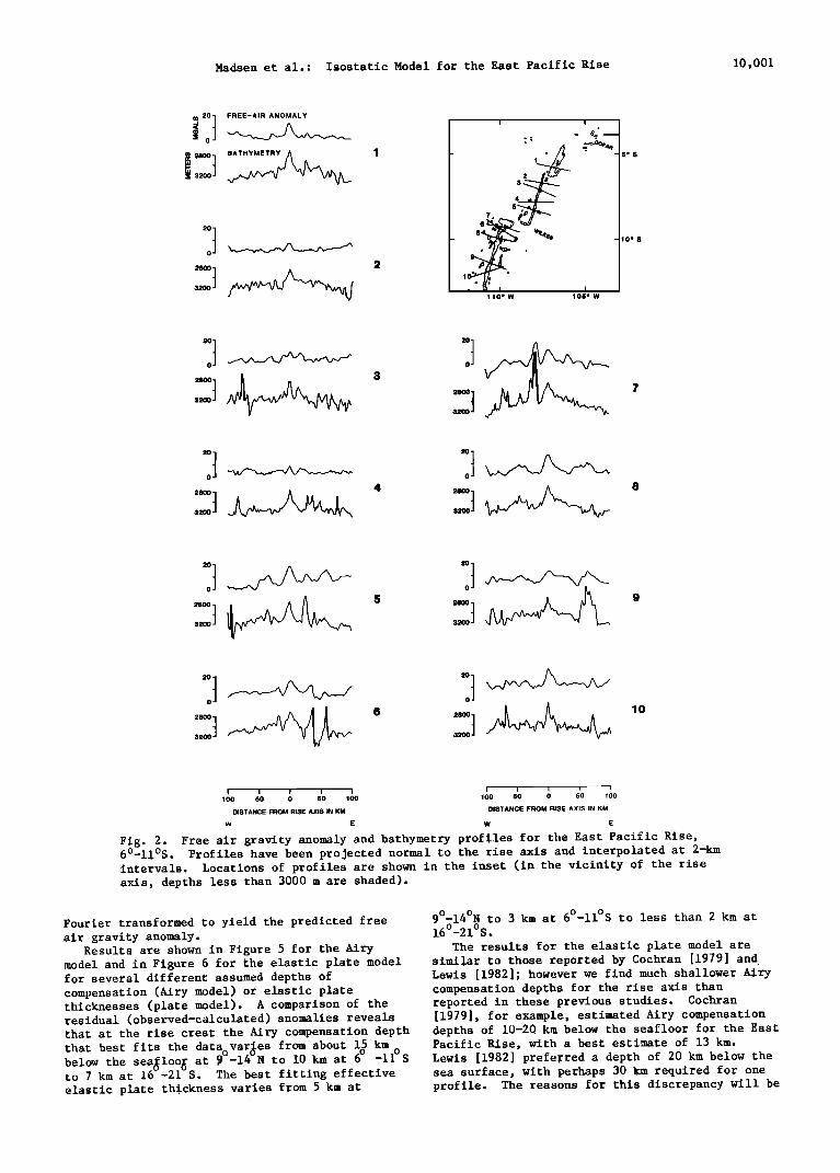
Fig. 2. Free air gravity anomaly and bathymetry profiles for the East Pacific Rise, 6ø-11øS. Profiles have been projected normal to the rise axis and interpolated at 2-km intervals. Locations of profiles are shown in the inset (in the vicinity of the rise axis, depths less than 3000 m are shaded).

Fourier transformed to yield the predicted free air gravity anomaly.

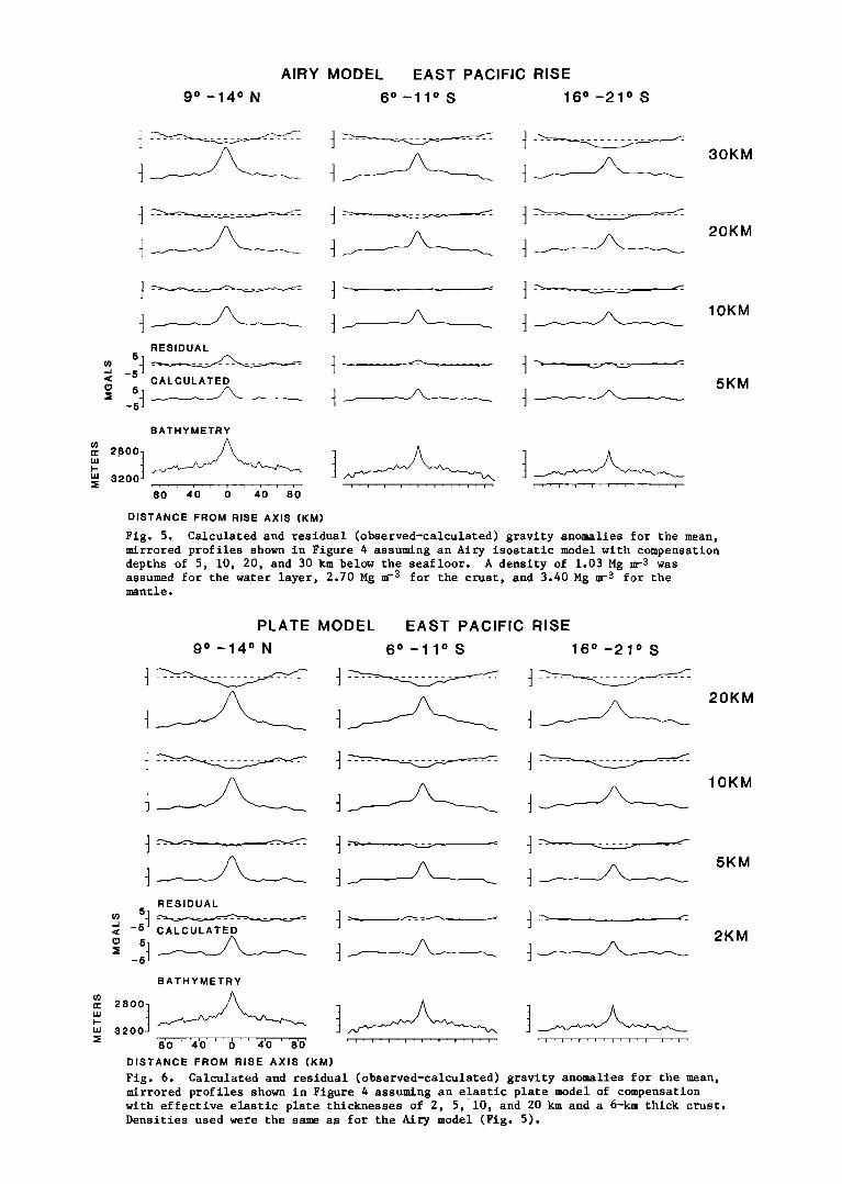
Results are shown in Figure 5 for the Airy model and in Figure 6 for the elasti c plate model for several different assumed depths of compensation (Airy model) or elastic plate thicknesses (plate model). A comparison of the

9ø-14øN to 3 km at 6ø-11øS to less than 2 km at 16ø-21øS.

The results for the elastic plate model are similar to those reported by Cochran [1979] and Lewis [1982]; however we find much shallower Airy compensation depths for the rise axis than reported in these previous studies. Cochran

residual (observed-calculated)anomalies reveals [1979], for example, estimated Airy compensation that at the rise crest the Airy compensation depth depths of 10-20 km below the seafloor for the East that best fits the data varies from about 15 km Pacific Rise, with a best estimate of 13 km. below the sea•1oo• at 9ø-14øN to 10 km at 6 ø -11øS Lewis [1982] preferred a depth of 20 km below the to 7 km at 16 -21 S. The best fitting effective sea surface, with perhaps 30 km required for one elastic plate th.ickness varies from 5 km at profile. The reasons for this discrepancy will be


30 t FREE-AIR ANOMALY 10

2800 .ATHY•ET• 1 3200

3o 2800 3200

ß

o 1

2 3

o • ß o

]o o

I 115 ø W 110 ø W

- 5os

- .•0 ø S

3o 2800 320O

3o t

30 t •o • 4 32OO

3o 2800 3200

3o 2800 3200

3200 3200

lO

I

,oo •'o g •'o ,go ,•o • • •'o ,go DISTANCE FROM RISE AXIS IN KM DISTANCE FROM RISE AXIS IN KM

W E W E

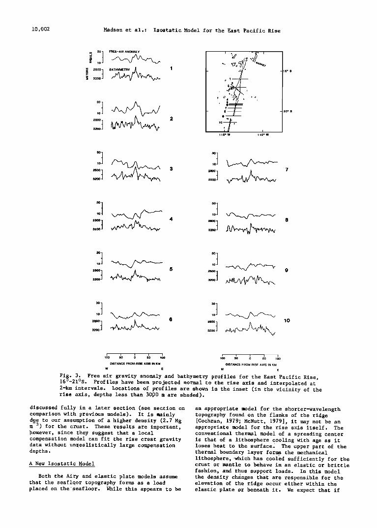
Fig. 3. Free air gravity anomaly and bathymetry profiles for the East Pacific Rise, 16ø-21øS. Profile• have been projected normal to the rise axis and interpolated at 2-km intervals. Locations of profiles are shown in the inset (in the vicinity of the rise axis, depths less than 3000 m are shaded).

discussed fully in a later section (see section on an appropriate model for the shorter-wavelength comparison with previous models). It is mainly topography found on the flanks of the ridge due to our assumption of a higher density (2.7 Mg m -3) for the crust. These results are important, how•ever, since they suggest that a local compensation model can fit the rise crest gravity data without unrealistically large compensation depths.

A New Isostatic Model

Both the Airy and elastic plate models assume that the seaflqor topography forms as a load placed on the •eafioor. While this appears to be

[Cochran, 1979; McNutt, 1979], it may not be an appropriate model for the rise axis itself. The conventional thermal model of a spreading center is that of a lithosphere cooling with age as it loses heat to the surface. The upper part of the thermal boundary layer forms the mechanical

,

lithosphere, 'which has cooled sufficiently for the crust or mantle to behave in an elastic or brittle

fashion, and thus support loads. In this model the density changes that are responsible for the elevation of the ridge occur either within the elastic plate or beneat h it. We expect that if


MEAN MIRRORED PROFILES EAST PACIFIC RISE

9 ø -14 ø N

6ø-11 ø S

FREE-AIR ANOMALY o3 20

o3 2800 :2 3200

16 ø -21 ø S

410 810 8 0 4•0 •) I

DISTANCE FROM RISE AXIS (KM)

Fig. 4. Mean, mirrored free air gravity anomaly and bathymetry profiles for the East Pacific Rise, 9ø-14øN, 6ø-11øS, and 16ø-21øS. Individual profiles from each region have been stacked (summed), and the mean profiles have been mirrored by summing half profiles from each side of the rise axis. Dashed line on the bathymetry profiles is the /t depth-age relation of Parsons and Sclater [1977].

there is a low-density magma chamber beneath the injection, we represent the mechanical response of axial high, it will exert an upward, buoyant force the seafloor by a plate broken at the ridge crest. on the bottom of the thin elastic plate that To explor e the importance of lateral variations in describes the mechanical behavior of the uppermost plate thickness, we will also examine plates crust. An appropriate model for the axial high, loaded from below that are not broken at the axis therefore, is the deflection of a floating elastic or that vary in flexural rigidity as a function of plate by a force on the base of the plate, not distance from the ridge axis. deflection of an elastic plate by topographic To find the response of this model to a load, loads placed on top of the plate. we need to solve the eq.uation for the deflection

In Figure 7 we schematically illustrate the w(x) of a thin, floating, elastic plate subject to differences between the response of this new model a load q(x), to a load and the response of conventional Airy and elastic plate models. In the latter models, elevated topography is treated as a load that is compensated at depth by a low-density root usually or associated with an increase in depth to the crust-mantle boundary (the largest density interface). In the model we propose, the axial topography is elevated by a buoyant force acting on the bottom of a thin elastic plate with a constant thickness crust. Since we expect the plate to •e very weak at the site of dike

d 2 d2w q(x) = •x2(D d-• ) + g(0m-0w)W(X)

, , d•w dD {d q(x) = •x)• + 2(•)•,,•-•, + O•D a•

(d•) (•2) + g(pm-Pw)w(x)

(la)

(lb)

where D(x) is the flexural rigidity and g is the

9 ø -14 ø N

AIRY MODEL EAST PACIFIC RISE

6 ø -11 ø S 16 ø -21 ø S

30KM

20KM

RESIDUAL

• -5 • CALCULATED

-5

10KM

5KM

2800

3200

BATHYMETRY

'8'0' ' '4'0 0 ' '4'0' ' '8'0' ß [ , [ , , , [ , [ , [ . ! . [ , [ . ß i ß [ ß i . i , i ß [ ß i ß i , i ,

DISTANCE FROM RISE AXIS (KM)

Fig. 5. Calculated and residual (observed-calculated) gravity anomalies for the mean, mirrored profiles shown in Figure 4 assuming an Airy isostatic model with compensation depths of 5, 10, 20, and 30 km below the seafloor. A density of 1.03 Mg m-3 was assumed for the water layer, 2.70 Mg m -3 for the crust, and 3.40 Mg m -• for the mantle.

PLATE MODEL EAST PACIFIC RISE

9 ø -14 ø N 6 ø -11 ø S 16 ø -21 ø S

10KM

RESIDUAL

03 ,5• ............ _1 -5 • CALCULATED

:• _5 • BATHYMETRY

n- 28001 m 3200

=" '8'0' ' '4'0'' 'O'' '4'0' ' '8'd DISTANCE FROM RISE AXIS (KM)

' , ß i , i ' i , , , i , i , i , i ,

Fig. 6. Calculated and residual (observed-calculated) gravity anomalies for the mean, mirrored profiles shown in Figure 4 assuming am elastic plate model of compensation with effective elastic plate thicknesses of 2, 5, 10, and 20 km and a 6-km thick crust. Densities used were the same as for the Airy model (Fig. 5).

5KM

2KM


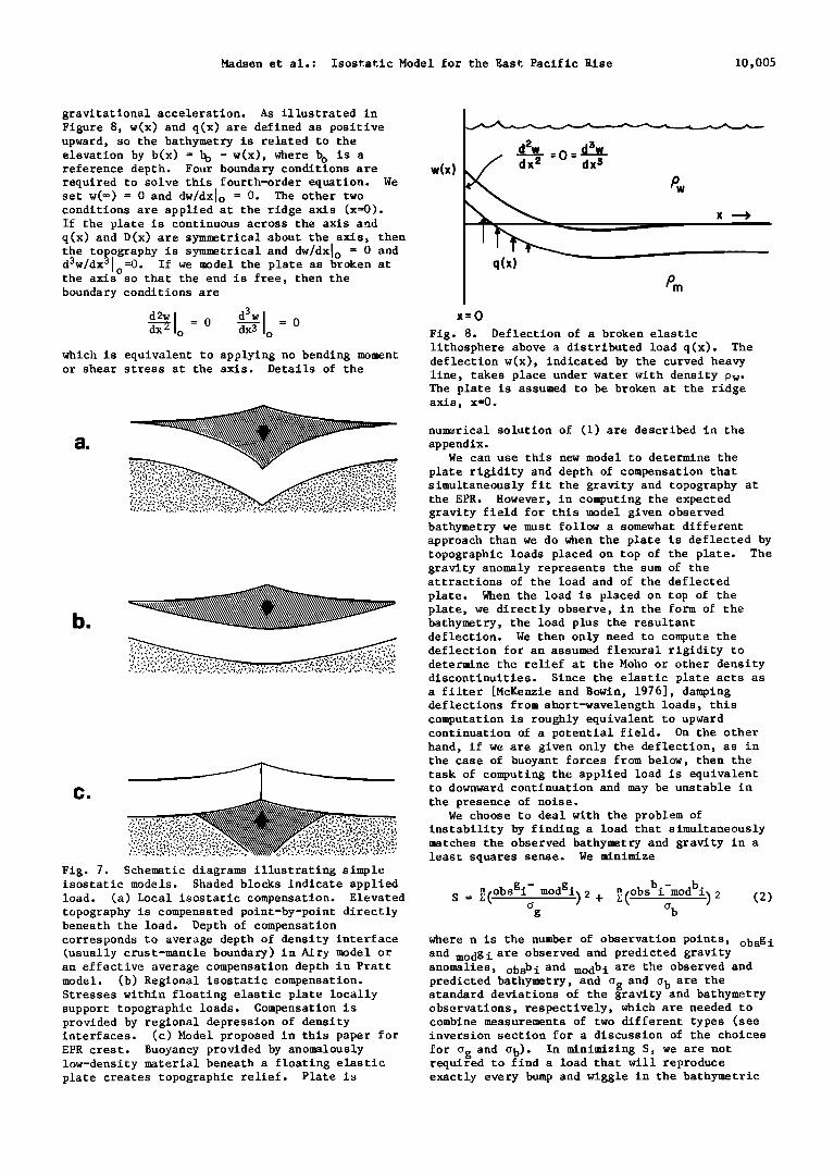
gravitational acceleration. As illustrated in Figure 8, w(x) and q(x) are defined as positive upward, so the bathymetry is related to the elevation by b(x) = b o -w(x), where b o is a reference depth. Four boundary conditions are required to solve this fourth-order equation. We set w(©) = 0 and dw/dxlo = 0. The other two conditions are applied at the ridge axis (x=O). If the plate is continuous across the axis and q(x) and D(x) are symmetrical about the axis, then the topography is symmetrical and dw/dxlo TM 0 and d3w/dxø1o=O. If we model the plate as broken at the axis so that the end is free, then the boundary conditions are

d3w d2w = 0 d-•l = 0 '•x'x •-- Jo o

which is equivalent to applying no bending moment or shear stress at the axis. Details of the

•m

bm

Fig. 7. Schematic diagrams illustrating simple isostatic models. Shaded blocks indicate applied load. (a) Local isostatic compensation. Elevated topography is compensated point-by-point directly beneath the load. Depth of compensation corresponds to average depth of density interface (usually crust-mantle boundary) in Airy model or an effective average compensation depth in Pratt model. (b) Regional isostatic compensation. Stresses within floating elastic plate locally support topographic loads. Compensation is provided by regional depression of density interfaces. (c) Model proposed in this paper for EPR crest. Buoyancy provided by anomalously low-density material beneath a floating elastic plate creates topographic relief. Plate is

w(x)

q(x)

x--O

Fig. 8. Deflection of a broken elastic lithosphere above a distributed load q(x). The deflection w(x), indicated by the curved heavy line, takes place under water with density Pw- The plate is assumed to be broken at the ridge axis, x=O.

numerical solution of (1) are described in the appendix.

We can use this new model to determine the

plate rigidity and depth of compensation that simultaneously fit the gravity and topography at the EPR. However, in computing the expected gravity field for this model given observed bathymetry we must follow a somewhat different approach than we do when the plate is deflected by topographic loads placed on top of the plate. The gravity anomaly represents the sum of the attractions of the load and of the deflected

plate. When the load is placed on top of the plate, we directly observe, in the form of the bathymetry, the load plus the resultant deflection. We then only need to compute the deflection for an assumed flexural rigidity to determine the relief at the Moho or other density discontinuities. Since the elastic plate acts as a filter [McKenzie and Bowin, 1976], damping deflections from short-wavelength loads, this computation is roughly equivalent to upward continuation of a potential field. On the other hand, if we are given only the deflection, as in the case of buoyant forces from below, then the task of computing the applied load is equivalent to downward continuation and may be unstable in the presence of noise.

We choose to deal with the problem of instability by finding a load that simultaneously matches the observed bathymetry and gravity in a least squares sense. We minimize

S = [( 'øbsgi- mødgi) 2 + •.(øbsbi-mødbi) 2 •g •b

(2)

where n is the number of observation points, obsgi and modgi are observed and predicted gravity anomalies, obsbi and modbi are the observed and predicted bathymetry, and o• and gb are the standard deviations of the gravity and bathymetry observations, respectively, which are needed to combine measurements of two different types (see inversion section for a discussion of the choices

for gg and •b)' In minimizing S we are not required to find a load that will reproduce exactly every bump and wiggle in the bathymetric


IO

GRAVITY

9 ø - 14 ø N

2.5 •,•.•,• _ BATHYMETRY ,, 3.0 ' -'-'- - -'-'-

3.5 0 20 40 60 80

DISTANCE FROM CREST km

I00

-3O

GRAVITY

6 ø -II ø S

2.5

r• BATHYMETRY

3.o[---•_-..•: = - : -__•_- L ß ' ' ' ' ' ' 60 80 I00


-3O

2.5

GRAVITY

16 ø- 21 ø S

r,• BATHYMETRY 3.0 ............

35 I , , , ß 0 20 40 610 • I 8•0 ioo

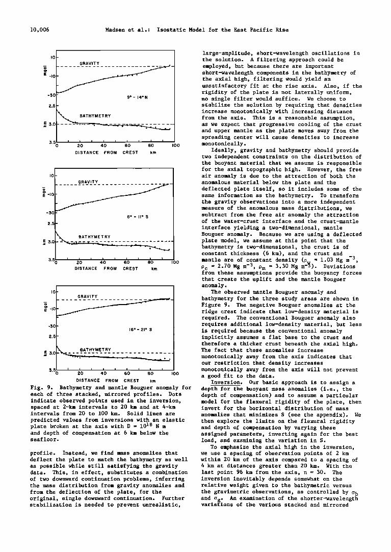
large-amplitude, short-wavelength oscillations in the solution. A filtering approach could be employed, but because there are important short-wavelength components in the bathymetry of the axial high, filtering would yield an unsatisfactory fit at the rise axis. Also, if the rigidity of the plate is not laterally uniform, no single filter would suffice. We choose to stabilize the solution by requiring that densities increase monotonically with increasing distance from the axis. This is a reasonable assumption, as we expect that progressive cooling of the crust and upper mantle as the plate moves away from the spreading center will cause densities to increase monotonically.

Ideally, gravity and bathymetry should provide two independent constraints on the distribution of the buoyant material that we assume is responsible for the axial topographic high. However, the free air anomaly is due to the attraction of both the anomalous material below the plate and the deflected plate itself, so it includes some of the same information as the bathymetry. To transform the gravity observations into a more independent measure of the anomalous mass distributions, we subtract from the free air anomaly the attraction of the water-crust interface and the crust-mantle

interface yielding a two-dimensional, mantle Bouguer anomaly. Because we are using a deflected plate model, we assume at this point that the bathymetry is two-dimensional, the crust is of constant thickness (6 kin), and the crust and mantle are of constant density (p 1.03 Mg m -3 Pc = 2.70 Mg m -3, Pm = 3.30 Mg •-•)7 Deviations' from these assumptions provide the buoyancy forces that create the uplift and the mantle Bouguer anomaly.

The observed mantle Bouguer anomaly and bathymetry for the three study areas are shown in Figure 9. The negative Bouguer anomalies at the ridge crest indicate that low-density material is required. The conventional Bouguer anomaly also requires additional low-density material, but less is required because the conventional anomaly implicitly assumes a flat base to the crust and therefore a thicker crust beneath the axial high. The fact that these anomalies increase

monotonically away from the axis indicates that our restriction that density increases monotonically away from the axis will not prevent a good fit to the data.

DISTANCE FROM CREST km Inversion. Our basic approach is to assign a Fig. 9. Bathymetry and mantle Bouguer anomaly for depth for the buoyant mass anomalies (i.e., the each of three stacked, mirrored profiles. Dots indicate observed points used in the inversion, spaced at 2-km intervals to 20 km and at 4-km intervals from 20 to 100 km. Solid lines are

predicted values from inversions with an elastic plate broken at the axis with D -- 1018 N m and depth of compensation at 6 km below the seafloor.

profile. Instead, we find mass anomalies that

depth of compensation) and to assume a particular model for the flexural rigidity of the plate, then invert for the horizontal distribution of mass

anomalies that minimizes S (see the appendix). We then explore the limits on the flexural rigidity and depth of compensation by varying these assigned parameters, inverting again for the best load, and examining the variation in S.

To emphasize the axial high in the inversion, we use a spacing of observation points of 2 km

deflect the plate to match the bathymetry as well within 20 km of the axis compared to a spacing of as possible while still satisfying the gravity data. This, in effect, substitutes a combination of two downward continuation problems, inferring the mass distribution from gravity anomalies and from the deflection of the plate, for the original, single downward continuation. Further stabilization is needed to prevent unrealistic,

4 km at distances greater than 20 km. With the last point 96 km from the axis, n = 30. The inversion inevitably depends somewhat on the relative weight given to the bathymetric versus the gravimetric observations, as controlled by •b and •g' An examination of the shorter-wavelength varia[ions of the various stacked and mirrored


0 ! .

, 9 ø- 14 ø N 6 ø -II ø S

Iog•oO N rn Iog[oO N rn Iog[oO N rn 18 19 20 17 18 19 20 17 18 19

i ß

I I

16 •- 21 • S

200

ß 12

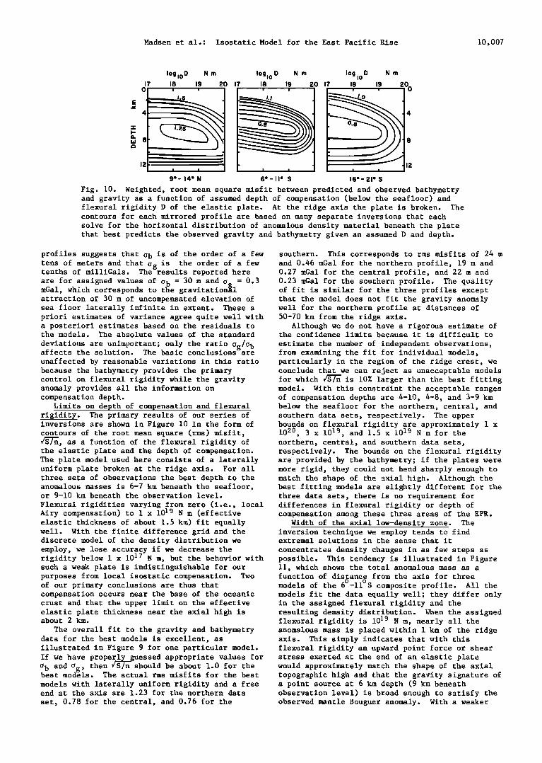
Fig. 10. Weighted, root mean square misfit between predicted and observed bathymetry and gravity as a function of assumed depth of compensation (below the seafloor) and flexural rigidity D of the elastic plate. At the ridge axis the plate is broken. The contours for each mirrored profile are based on many separate inversions that each solve for the horizontal distribution of anomalous density material beneath the plate that best predicts the observed gravity and bathymetry given an assumed D and depth.

profiles suggests that Ob is of the order of a few southern. This corresponds to rms misfits of 24 m tens of meters and that Og is the order of a few and 0.46 mGal for the northern profile, 19 m and tenths of milliGals. The results reported here 0.27 mGal for the central profile, and 22 m and

are for assigned values of o b = 30 m and Og = 0.3 0.23 mGal for the southern profile. The quality mGal, which corresponds to the gravitational of fit is similar for the three profiles except attraction of 30 m of uncompensated elevation of that the model does not fit the gravity anomaly sea floor laterally infinite in extent. These a well for the northern profile at distances of priori estimates of variance agree quite well with 50-70 km from the ridge axis. a posteriori estimates based on the residuals to the models. The absolute values of the standard

deviations are unimportant; only the ratio Og/O b affects the solution. The basic conclusions are

unaffected by reasonable variations in this ratio because the bathymetry provides the primary control on flexural rigidity while the gravity anomaly provides all the information on compensation depth.

Limits on depth of compensation and flexural ri$idity. The primary results of our series of inversions are shown in Figure 10 in the form of contours of the root mean square (rms) misfit, /S/n, as a function of the flexural rigidity of the elastic plate and the depth of compensation. The plate model used here consists of a laterally uniform plate broken at the ridge axis. For all three sets of observations the best depth to the anomalous masses is 6-7 km beneath the seafloor, or 9-10 km beneath the observation level.

Although we do not have a rigorous estimate of the confidence limits because it is difficult to

estimate the number of independent observations, from examining the fit for individual models, particularly in the region of the ridge crest, we conclude that we can reject as unacceptable models for which • is 10% larger than the best fitting model. With this constraint the acceptable ranges of compensation depths are 4-10, 4-8, and 3-9 km below the seafloor for the northern, central, and southern data sets, respectively. The upper bounds on flexural rigidity are approximmtely 1 x 1020, 3 x 1019, and 1.5 x 1019 N m for the northern, central, and southern data sets, respectively. The bounds on the flexural rigidity are provided by the bathymetry; if the plates were more rigid, they could not bend sharply enough to match the shape of the axial high. Although the best fitting models are slightly different for the three data sets, there is no requirement for

Flexural rigidities varying from zero (i.e., local differences in flexural rigidity or depth of Airy compensation) to 1 x 1019 N m (effective compensation among these three areas of the EPR. elastic thickness of about 1.5 km) fit equally Width of the axial low-density zone. The well. With the finite difference grid and the inversion technique we employ tends to find discrete model of the density distribution we extremal solutions in the sense that it employ, we lose accuracy if we decrease the concentrates density changes in as few steps as rigidity below 1 x 1017 N m, but the behavior with possible. This tendency is illustrated in Figure such a weak plate is indistinguishable for our purposes from local isostatic compensation. Two of our primary conclusions are thus that compensation occurs near the base of the oceanic crust and that the upper limit on the effective elastic plate thickness near the axial high is about 2 km.

The overall fit to the gravity and bathymetry data for the best models is excellent, as illustrated in Figure 9 for one particular model.

11, which shows the total anomalous mass as a function of distance from the axis for three

models of the 6ø-11øS composite profile. All the models fit the data equally well; they differ only in the assigned flexural rigidity and the resulting density distribution. When the assigned flexural rigidity is 1019 N m, nearly all the anomalous mmss is placed within 1 km of the ridge axis. This simply indicates that with this flexural rigidity an upward point force or shear

If we have properly guessed appropriate values for stress exerted at the end of an elastic plate o and o_ t e ' / should be about 1.0 for the would approximately match the shape of the axial b •, hn/Sn best models. The actual rms misfits for the best topographic high and that the gravity signature of models with laterally uniform rigidity and a free a point source at 6 km depth (9 km beneath end at the axis are 1.23 for the northern data observation level) is broad enough to satisfy the set, 0.78 for the central, and 0.76 for the observed mantle Bouguer anomaly. With a weaker


I

E 2.O

O.O O

6 ø- II0 S

Depth 6 km

...... I0 •9 N m 18

1017

.................. J ..... ; .... t,tttt--'t .................... i

io 20 $o


results of inversions with depth and rigidity the same for all three regions (Figure 13) suggest that the amplitude of the mass anomaly at the ridge crest may remain roughly constant from one region to the next but that either the width of the anomalous low-density zone is variable or the volume of anomalous material outside the immediate

axis area but still within 15 km of the axis

varies from region to region. Is the plate broken at the ridge axis?

Although our preferred model is a plate that is very weak or broken at the ridge axis, but possessing significant flexural rigidity elsewhere, there is clearly no requirement within our data for the plate to be any different at the ridge crest because a model with zero flexural rigidity everywhere is acceptable. We have explored whether the upper limit on D varies with

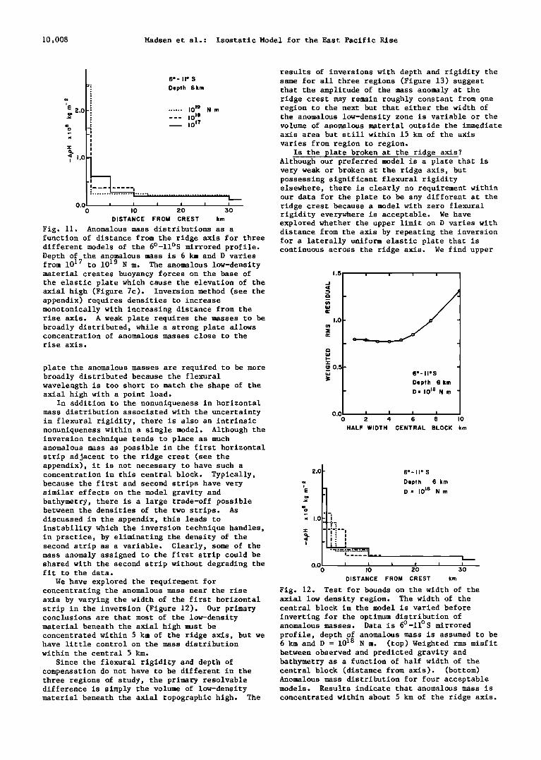
Fig. 11. Anomalous mass distributions as a distance from the axis by repeating the inversion function of distance from the ridge axis for three for a laterally uniform elastic plate that is different models of the 6ø-11øS mirrored profile. continuous across the ridge axis. We find upper Depth of the anomalous mass is 6 km and D varies from 1017 to 1019 N m. The anomalous low-density material creates buoyancy forces on the base of the elastic plate which cause the elevation of the axial high (Figure 7c). Inversion method (see the appendix) requires densities to increase monotonically with increasing distance from the rise axis. A weak plate requires the masses to be broadly distributed, while a strong plate allows concentration of anomalous masses close to the

rise axis.

plate the anomalous masses are required to be more broadly distributed because the flexural wavelength is too short to match the shape of the axial high with a point load.

In addition to the nonuniqueness in horizontal mass distribution associated with the uncertainty in flexural rigidity, there is also an intrinsic nonuniqueness within a single model. Although the inversion technique tends to place as much anomalous mass as possible in the first horizontal strip adjacent to the ridge crest (see the appendix), it is not necessary to have such a concentration in this central block. Typically, because the first and second strips have very similar effects on the model gravity and bathymetry, there is a large trade-off possible between the densities of the two strips. As discussed in the appendix, this leads to instability which the inversion technique handles, in practice, by eliminating the density of the second strip as a variable. Clearly, some of the mass anomaly assigned to the first strip could be shared with the second strip without degrading the fit to the data.

We have explored the requirement for concentrating the anomalous mass near the rise axis by varying the width of the first horizontal strip in the inversion (Figure 12). Our primary conclusions are that most of the low-density material beneath the axial high must be

1.5

hi

•0.5-

0.0. 0

6 ø- II ø S

Depth 6 km

D- I018 N m

i i I i

2 4 6 8 I0

HALF WIDTH CENTRAL BLOCK km

2.ø t 'E J Depth 6 km

• • D = I0 •8 N m : •.o1:.1'i

I: I 0.0

0 I0 20 $0


Fig. 12. Test for bounds on the width of the axial low density region. The width of the central block in the model is varied before

inverting for the optimum distribution of anomalous masses. Data is 6ø-11 ø S mirrored

concentrated within 5 km of the ridge axis, but we profile, depth of anomalous mass is assumed to be have little control on the mass distribution 6 km and D = 1018 N m. (top) Weighted rms misfit within the central 5 km.

Since the flexural rigidity and depth of compensation do not have to be different in the three regions of study, the primary resolvable difference is simply the volume of low-density material beneath the axial topographic high. The

between observed and predicted gravity and bathymetry as a function of half width of the central block (distance from axis). (bottom) Anomalous mass distribution for four acceptable models. Results indicate that anomalous mass is

concentrated within about 5 km of the ridge axis.


limits on flexural rigidity ranging from 1 to 3 x 1018 N m for the three profiles, an order of magnitude or more smaller than the limits for a broken plate. The upper limit on effective elastic thickness, therefore, must be lower near the axis.

We have also performed inversions for models in which the flexural rigidity varies with distance from the ridge axis. This brings into play the second and third terms in equation (lb). Ideally, D and its first and second derivatives should be

analytically continuous, well-behaved functions. In the finite difference formulation, as long as D(x) and dD/dx are analytically continuous and d 2D/dx 2 is estimated by finite differences from D, then the solution is stable and accurate. As a

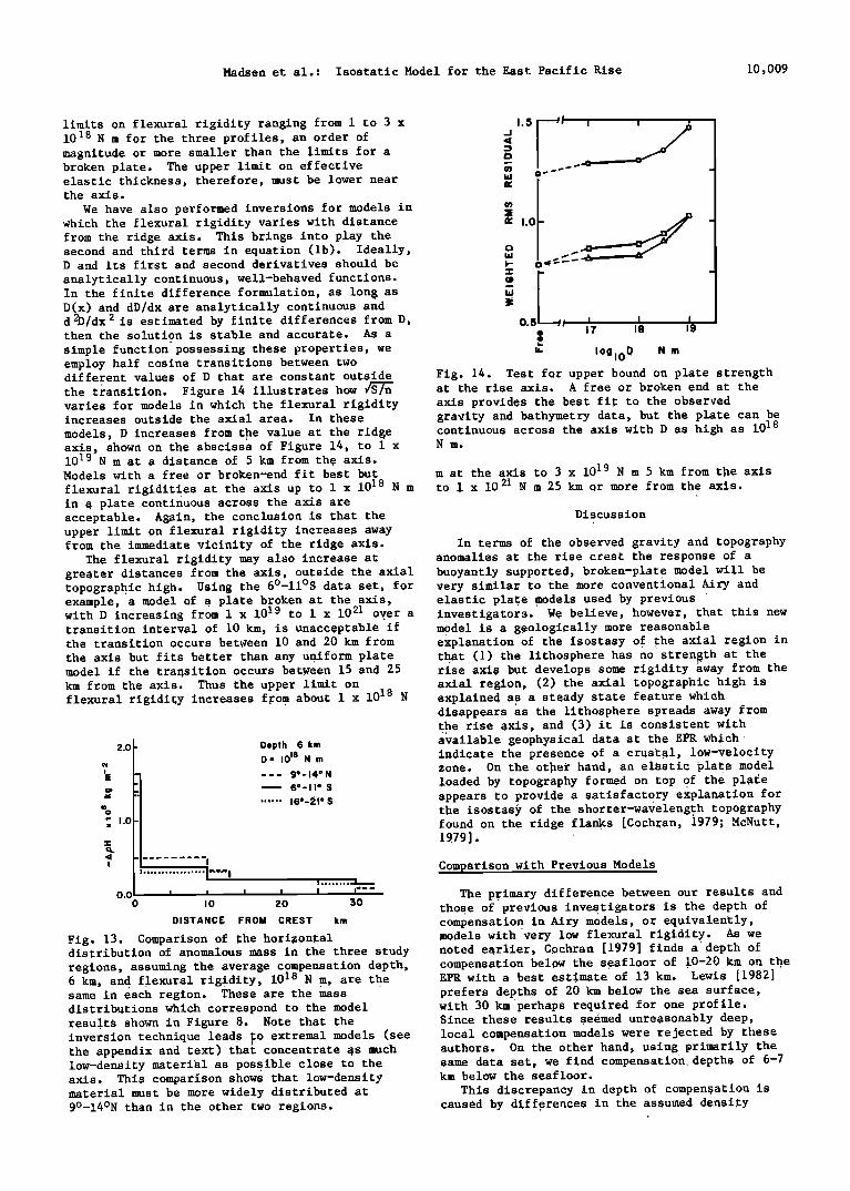
simple function posse•ssing these properties, we employ half cosine transitions between two different values of D that are constant outside the transition. Figure 14 illustrates how • varies for models in which the flexural rigidity increases outside the axial area. In these

models, D increases from t•he value at the ridge axis, shown on the abscissa of Figure 14, to 1 x 1019 N m at a distance. of 5 km from the axis.

0.5 :I I I I _ 17 18 19

u. log i0 D N m Fig. 14. Test for upper bound on plate strength at the rise axis. A free or broken end at the

axis provides the best fit to the observed gravity and bathymetry data, but the plate can be continuous across the axis with D as high as 1018 N m.

Models with a free or broken-end fit best but m at the axis to 3 x 1019 N m 5 km from th e axis flexural rigidities at the axis up to 1 x 1018 N m to 1 x 1021 N m 25 km or more from the axis. in a plate continuous across the axis are acceptable. Again, the conclusion is that the Discussion upper limit on flexural rigidity increases away from the immediate vicinity of the ridge axis. In terms of the observed gravity and topography

The flexural rigidity may also increase at anomalies at the rise crest the response of a greater distances from the axis, outside the axial buoyantly supported, broken-plate model will be topographic high. Using the 6ø-11øS data set, for very similar to the more conventional Airy and example, a model of a plate broken at the axis, elastic plat e models used by previous with D increasing from 1 x 1019 to 1 x 10 21 over a investigators. We believe, however, that this new transition interval of 10 km, is Unacceptable if the transition occurs between 10 and 20 km from the axis but fits better than any un•iform plate model if the transition occurs between 15 and 25 km from the axis. Thus the upper limit on flexural rigidity increases from about 1 x 1018 N

2.0 Depth 6 km

D = I0 i8 N m ___ 9o- 14o N

6ø-II ø S

...... 16ø-21 ø S

o.o , , , , i ";--- o io 20 30


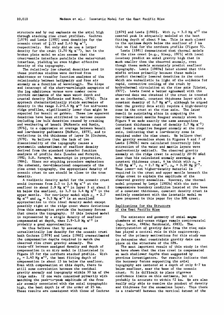
Fig. 13. Comparison of the horizontal distribution of anomalous mass in the three study regions, assuming the average compensation depth, 6 km, and flexural rigidity, 1018 N m, are the same in each region. These are the mass distributions which correspond to the model results shown in Figure 8. Note that the inversion technique leads •o extremal models (see the appendix and text) that concentrate •s much low-density material as possible close to the axis. This comparison shows that low-density material must be more widely distributed at 9ø-14øN than in the other two regions.

model is a geologically more reasonable explanation of the isos•tasy 0•f •he axial region in that (1) the lithosphere has no' strength at the rise axis but develops som e rigidity •way from the axial region, (2) the axial topographic high is explained as a steady state feature which disappears as the lithosphere Spreads away from the rise axis, and (3) it is consistent with available geophysical data at the EPR wh$ch indicate the presence of a crust•al, low-velocity zone. On the oth er hand, an elastic •late model loaded 5Y topography formed on top of the pla•e appears to provide a satisfactory explanation for the isostas• of the shorter-wavelength topography found on the ridge flanks [Cochran, 1979; McNutt, 1979].

Comparison with Previous Models

The primary difference between our results and those of previous investigators is the depth of compensatio n in Airy models, or equivalently, models with very low flexural rigidity. As we noted earlier, Cochran [!979] finds a depth of compensation below the seafloor of .10-20 km o n the EPR with a best estimate of 13 kin. Lewis [1982] prefers depth s of 20 km below the sea surface, with 30 km'perhaps required for one profile. Since these results se•med unreasonably deep,

local compensatio n models were rejected by these authors. On the other hand, using primarily the same data set, we find compensation, depths of 6-7 km below the seafloor.

This discrepancy in depth of compensation is caused by diff•erences in the assumed density


structure and by ou.r• emphasis on the axial high through stacking rise crest profiles. Cochran [1979] and Lewis [1982] used densities fqr the oceanic crust of • 33 and 2.43 Mg m -3 • respectively. Not only did w•e use a larger density for the cru•t (2.70 Mg m-3), but•in the broken plate model we also assume that the crust-mantle interface parallels the water-crust interface, yielding'•an even higher effective density of the topography.

The relatively low.•crustal densities used in these previous studies were derived from admittance or transfer function• analy•es of the relationship between •athymetry and free air

[1979] and Lewis [1982]. With Pc = 3.0 Mg m -3 the central peak is adequately modeled at the best fitting depth of about 9 km. This is much closer to the optimum depth below the seafloor of 7 km that we find fortthe northern profile (Figure 9).

Lewis [1981] demonstrated that thermal models of the .rise crest [e.g., Sleep, 1975] with local isostasy predict an axial gravity high that is much smaller then the observed anomaly, even though these models accurately predict seafloor topography. Lewis [1983b] later showed that this misfit arises primarily because these models predict thermally lowered densities in the crust which are unrealistic in light of the evidence for

anomaly as a function of Wavelength. The •1ope rapid, convec.tive coolin•g of the cru•t by and intercept of th.e short-wavele•gt h asymptote of hydrothermal circulation at the rise axis [Lister, the log admittance versus wave number curve 1977]. Lewis found a better agreemen• with the provide estimates of the mean wate r depth and observed data was obtained if the crust is treated crustal density [McKenzie and Bowin, 1976]. This as an isothermal, constant thickness layer with a approach characteristically yields. estimates of constant density of 2.7 Mg m -•, altho?gh he argued density in the range 2.2-2.4 Mg m -• fo• mid-ocean that the gravity data still require a high-density ridge profiles, significantly lower than might be zone in the crust at the rise axis. The later ex•pected for basalt or gabbro. These low apparent result is surprising since in computing the densities have been attributed to various causes

in•cluding low bul•densities caused by cracking and weathering of basalt [McKenzie and B•wi•n, 1976], to a c•mpromise or average between basalt and low-densit•y •ediments [McNutt, 1979], and to variations in th• thickness of layer 2A [Cochran, 1979]. We believe that the lack of two dimensionality oœ the topography causes a systematic underestimate of seafloor density derived from the standard transfer function

analysis of profile data [Louden and Forsyth, 1982• D.W. Forsyth, manuscript in preparation, 1984]. Since our sta•cking p.rocedure emphasizes the coherent, two-dimensional components of the rise crest topography, the appropriate density of oceanic crust to use should be close to the true

density.

.two-dimensional mantle Bouguer anomaly shown in Figure 9 we made exactly the same assumptions (constant thickness cru•t of density 2.7 Mg m -•) and found a negative Bouguer anomaly at the rise axis, indicating that a low-density zone is required under the rise crest. We believe that the g•ravity anomalies shown in Figures 6 and 7 of Lewis [1983b] were calculated incorrectly (the attraction of the water and .mantle layers were inadvertently omitted). The observed gravity anomaly at the ridge crest is actually 20-30 mGal less than his calculated anomaly assuming a constant thickness crust, 6 km thick with 0w = 1.03 Mg m -•, 0c = 2.7 Mg m -3, Pw = 3.30 Mg •m -•. Thus lower- not higher-density ma•terial is • required in the crust and upper mantle beneath the ridge crest to explain the amplitude of the

A realistic density model for the oceanic crust observed gravity anomalies. However, the thermal would increase from 2.3 to 2.4 Mg m -• at the model proposed by Lew•s [1983b] with the zero seafloor to about 2.9 Mg m -• in layer 3 at about 2 temperature boundary condition located at the base km below the seafloor, to 3.3 to 3.4 Mg m -• in the of a constant thickness, constant density crust is upper mantle. Our two-layer model with 0• = 2.7 entirely consistent with the •sostatic model we

' %.

Mg m -• and 0m = 3.3 Mg m -3 is an excellent have proposed in this pap,er for the EPR crest. approximation to this ideal density model except possibly right at the ridge crest where deviations Implications for the Structure from this assumption provide the buoyancy forces that create the topography. If this layered model is represented by a single density of seafloor compensated at depth, then 2.9-3.0 Mg m -3 is probably a good approximation.

We thus believe that by assuming an unrealistically low density for the oceanic crust

of the East Pacific Rise

The existence and geometry of axial magma chambers at mid-ocean ridges remain controversial [eg., Lewis, 1983a; Macdonald, 1983]. The• interpretation of gravity data from the ris• axis has played a central role in this controversy.

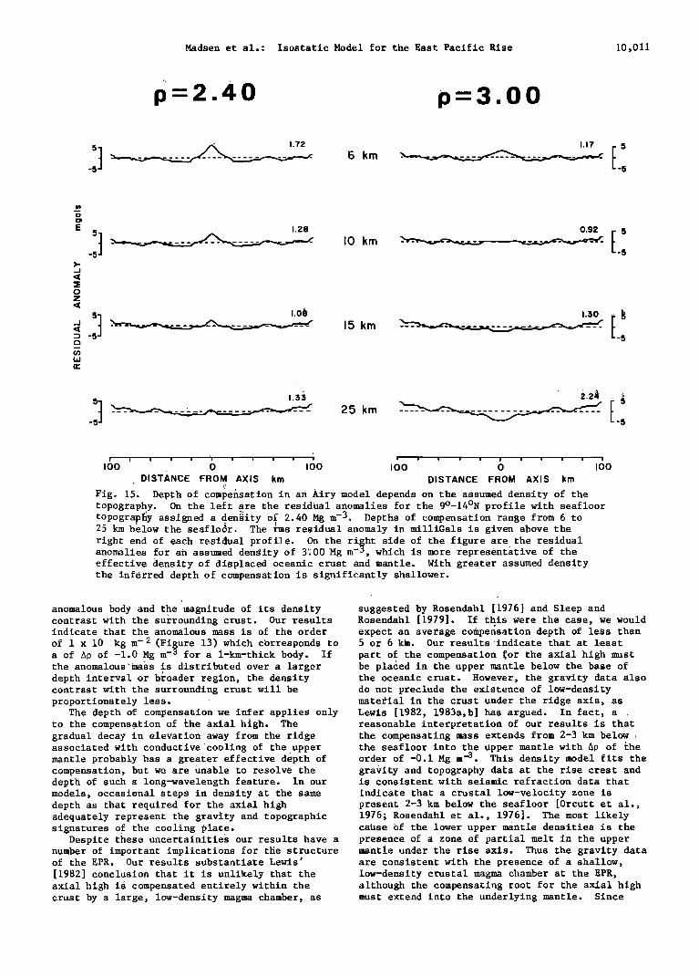
both Cochran [1979] and Lewis [1982] overestimated One of the primary motivations for this stud• was the compensation depths required to match the observed rise crest gravity anomaly. The trade-off between assigned density and depth of compensation in an Airy model is illustrated in Figure 15 for the northern stacked profile. With 0c = 2 40 Mg m -• the best fitting depth of compensation is about 15 km below the s•eafloor. Even with compensation at this depth, there is still some correlation between the residual

to dete.rmine what constraints gravity data can place on the structure of the EPR.

The most important result of ghis study is that we have shown that the rise crest is compensated at much shallower depths than suggested by previous investigators. Our results indicate that the buoyancy forces supporting the axial topography are centered at a depth of only 6-7 km below seafloor, near the base of the oceanic

gravity anomaly and topography within 30 km of the crust. It is difficult to place rigorous ridge axis. If one were concerned primarily with confidence limits on this estimate, put it matching the peak-to-peak amplitude of the free probably is accurate to within ñ2 km. We are also air anomaly associated with the axial topographic really only able to resolve the product of density high, the best depth is of the order of 25 km. and thickness for •h• anomalous layer. Th•s there These results are consistent with those of Cochran is a trade-off between the vertical •xtent of the


p=2.40 p-3.00

1.17

B km ...........

5 1.28

5 •.o•

:;3 -5

0.92

I0 km ..............

15 km

5 I'$•$ ':: 2'2'•"• • ................. 25 km •_.._ -'""•"•"•'•--' • .•.•...•.•.:•_._._ 5

-.5 -,5

i ! ! ! ! • ! ! ! ! ! ! ' ' ' ,oo ,6o '

DISTANCE FROM AXIS km DISTANCE FROM AXIS km '"

Fig. 15. Depth of compensation in an Airy model depends on the assumed density of the topography. On the left are the residual anomalies for the 9ø-14øN profile with seafloor topogra.p•y assigned a •en;•ity• o• 2.40 Mg m -3. Depths of compensation range from 6 to 25 km below the seaflod r. The rms residual anomaly in miliiGals is given above the right end of each residual profile. On the right side of the figure are the residual anomalies for an assumed dengity of 3;•00 Mg m -ø, which is more representative of the effective density of displaced oceanic crust and mantle. With greater assumed density the inferred depth of compensation is significantly shallower.

anomalous body and the magnitude of its density suggested by Rosendahl [1976] and Sleep and contrast with the surrounding crust. Our results Rosendahl [1979]. If this were the case, we would indicate that the anomalous mass is of the' order expect an average compensation depth of less than of 1 x 10 kg m -2 (Figure 13) which corresponds to 5 or 6 k•. Our results •indicate that at least a of AO of -1.0 Mg m '3 for a 1-km-thick body. If part of the compensation •or the axial high must the anomalous • mass is distributed over a larger be placed in the upper mantle below the base of depth interval or b•oader region, the density the oceanic crust. However, the gravity data also contrast with the surrounding crust will be do not preclude the existence of low-density proportionately less. mmteCial in the crust under the ridge axis, as

The depth of compensation we infer applies only Lewis [1982, 1983a,b] has argued. In fact, a to the compensation of the axial high. The gradual decay in elevation away from the ridge associated With conductive cooling of the upper mantle probably has a greater effective depth of compensation, but we are unable to resolve the depth of such a long-wavelength feature. In our models, occasional steps in density at the same depth as that required for the axial high adequately represent the gravity and topographic

reasonable interpretation of our results is that the compensating mass extends from 2-3 km below the seafloor into the Upper mantle with AD of the order of -0.i Mg m -3. This density model fits the gravity and topography data at the rise crest and is consistent with seismic refraction data that

indicate that a crustal low-velocity zone is present 2-3 km below the seafloor [Orcutt et al., 1976; Rosendahl et al., 1976]. The most likely

signatures o• the cooling plate. cabse Of the lower upper mantle densities is the Despite these uncertainitie• our results have a presence of a zone of partial melt in the upper

number of important implications for the structure mantle under the rise axis. Thus the gravity data of the EPR. Our results substantiate Lewis' are consistent with the presence of a shallow, [1982] conclusion that it is unlikely that the low-density crustal magma chamber at the EPR, axial high i s compensated entirely within the although the compensating root for the axial high crust by a large, low-density magma chamber, as must extend into the underlying mantle. Since


DISTANCE FROM RiSE AXIS (KM)

24 t6 8 0 8 16 24 I I I I ! I I I I I I I

O-

2 -

D

E 4-

P

T 6-

H

(KM) 8-

10-

• PARTIAL MELT

" ß ß -•'-"-•'•"-'-*"'•'•*"""•'• ""--'"'•"•:-'7'•--•"'• "•----• EXTRUSIVE BASALTS

IIII IJ , sHEETEO o'KES =i '

• SEISMIC MOHO CUMULATE GABBROS

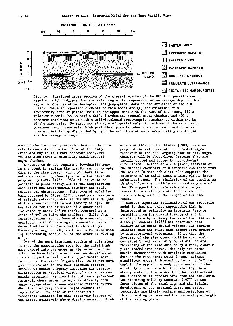
•-• ..... • ;• :•'•'-• ..... '•:•J o oø o .... ':?•'•:•: ............ ;• T E CTO Ni z ED H A R z B u R G I T E S Fig. 16. Idealized cross section of the crestal •ortion of the EPR incorporating our results, which indicate that the axial region is compensated at an average depth of 6-7 km, with other existing geological and geophysical data on the structure of the EPR crest. The most important elements of this model are (1) the existence of a low-density zone oftpartial melt in the' upper mantle at the base of the crust, (2) a relatively small (<4 km half width), low-density crustal magma chamber, and (3) a constant thickness crust with a well-developed crust-mantle boundary to within 2-3 km of the rise axis. We interpret the zone of partial melt at the base of the crust as a permanent magma reservoir which periodically replenishes a short-lived crustal magma chamber that is rapidly cooled by hydrothermal circulation between rifting events (2X vertical exaggeration).

most of the low-density material beneath the rise exists at this depth. Lister [1983] has also axis is concentrated within 5 km of the ridge proposed the existence of a subcrustal magma crest and may be in a much narrower zone, our reservoir at the EPR, arguing that crustal magma results also favor a relatively small crustal chambers will be short-lived features that are magma chamber. rapidly cooled and frozen by hydrothermal

However, we do not require a low-density zone circulation. Elthon et al.'s [1982] analysis of in the crust to explain the gravity and topography the mineral chemistry of uitramafic cumulates from data at the rise c•est. Although there is no the Bay of Islands ophiolite also supports the evidence for a high-density zone in the crust as existence of an axial magma chamber with a large proposed by Lewis [1982, 1983a,b], it would be subcrustal root. The similarity of the results we possible to place nearly all of the compensating obtained from three widely separated segmeats of mass below the crust-mantle boundary and still the EPR suggest that this subcrustal magma satisfy our observations. This type of model has reservoir is a steady state feature which is been proposed by Bibee [1979] based On an analysis present along most of the length of the rise of seismic refraction data at the EPR at 10os (one crest. of the areas included in our gravity study). He Another important implication of our isostatic has argued for the existence of a subcrustal model is that the axial topographic high is low-velocity zone, 2-3 km thick, centered at a interpreted as primarily an isostatic feature depth of 6-7 km below the seafloor. While this resulting from the upward flexure of a thin iaterpretation has not been widely accepted, it is elastic plate by buoyancy forces at the rise axis. consistent with the average compensation depth Although Lonsdale [1977] has described this determined for the rise crest in this study. feature as an axial shield volcano, our results However, a large density contrast is required with indicate that the axial high cannot form entirely the surrounding mantle (A0 of the order of -0.4 Mg by constructional volcanism. If it did, the

-3 m ). isostasy of the rise crest would be adequately One of the most important results of this study described by either an Airy model with crustal

is that the compensating root for the axial high thickening at the rise axis or by a weak, elastic must extend into the upper mantle below the rise plate loaded from above. Not only are these axis. We have interpreted these low densities as models inconsistent with available geophysical a zone of partial melt in the upper mantle near data at the rise crest which do not indicate the base of the crust (Figure 16). We do not have significant crustal thickening, but they fail to good constraints on the melt fraction present explain the apparent steady state nature of the because we cannot uniquely determine the density axial high. In our model the axial high is a distribution or vertical extent of this anomalous steady state feature since the plate will unbend mantle material. We view this body as a permanent and subside as it spreads away from the rise axis. reservoir where magma rising adiabatically from The fissuring noted by Lonsdale [1977] on the below accumulates between episodic rifting events lower slopes of the axial high and the initial when the overlying crustal magma chamber is development of the marginal horst and graben replenished. The base of the crust is a topography are likely surface manifestations of reasonable location for this reservoir because of this unbending process and the increasing strength the large, relatively sharp density contrast which of the cooling plate.


Conclusions

We have presented a new isostatic model for the crestal region of the East Pacific Rise. This model involves a thin, elastic plate, with a constant thickness crust, broken at the ridge crest. A buoyant force beneath the plate bends the free edge of the plate upward at the rise axis, forming a topographic high. Since both the seafloor and the crust-mantle boundary are elevated at the ridge crest a positive free air gravity anomaly is also present. This model is physically reasonable in that we assume that the

DISTANCE FROM AXIS ! !

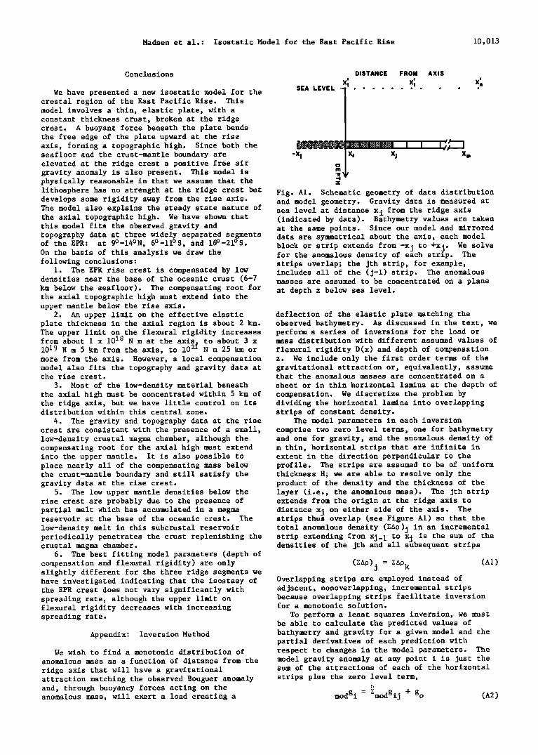
X I X i X• SEA LEVEL ............

Xl X I Xm

lithosphere has no strength at the ridge crest but Fig. A1. Schematic geometry of data distribution develops some rigidity away from the rise axis. and model geometry. Gravity data is measured at The model also explains the steady state nature of sea level at distance x i from the ridge axis the axial topographic high. We have shown that (indicated by data). Bathymetry values are taken this model fits the observed gravity and at the same points. Since our model and mirrored topography data at three widely separated segments data are symmetrical about the axis, each model of the EPR: at 9ø-14øN, 6ø-1•S, and 1•-2•S. block or strip extends from -xj to +xj. We solve On the basis of this analysis we draw the following conclusions:

1. The EPR rise crest is compensated by low densities near the base of the oceanic crust (6-7 km below the seafloor). The compensating root for the axial topographic high must extend into the upper mantle below the rise axis.

2. An upper limit on the effective elastic

for the anomalous density of each strip. The strips overlap; the jth strip, for example, includes all of the (j-l) strip. The anomalous masses are assumed to be concentrated on a plane at depth z below sea level.

deflection of the elastic plate matching the plate thickness in the axial region is about 2 km. observed bathymetry. As discussed in the text, we The upper limit on the flexural rigidity increases perform a series of inversions for the load or from about 1 x 1018 N m at the axis. to about 3 x mass distribution with different assumed values of 1019 N m 5 km from the axis, to 102f N m 25 km or flexural rigidity D(x) and depth of compensation more from the axis. However, a local compensation z. We include only the first order terms of the model also fits the topography and gravity data at gravitational attraction or, equivalently, assume the rise crest. that the anomalous masses are concentrated on a

3. Most of the low-density material beneath sheet or in thin horizontal lamina at the depth of the axial high must be concentrated within 5 km of compensation. We discretize the problem by the ridge axis, but we have little control on its dividing the horizontal lamina into overlapping distribution within this central zone. strips of constant density.

4. The gravity and topography data at the rise The model parameters in each inversion crest are consistent with the presence of a small, comprise two zero level terms, one for bathymetry low-density crustal magma chamber, although the compensating root for the axial high must extend into the upper mantle. It is also possible to place nearly all of the compensating mass below the crust-mantle boundary and still satisfy the gravity data at the rise crest.

5. The low upper mantle densities below the rise crest are probably due to the presence of partial melt which has accumulated in a magma reservoir at the base of the oceanic crest. The

low-density melt in this subcrustal reservoir periodically penetrates the crust replenishing the crustal magma chamber.

6. The best fitting model parameters (depth of compensation and flexural rigidity) are only slightly different for the three ridge segments we have investigated indicating that the isostasy of the EPR crest does not vary significantly with spreading rate, although the upper limit on flexural rigidity decreases with increasing spreading rate.

Appendix: Inversion Method

We wish to find a monotonic distribution of anomalous mass as a function of distance from the

ridge axis that will have a gravitational attraction matching the observed Bouguer anomaly and, through buoyancy forces acting on the anomalous mass, will exert a load creating a

and one for gravity, and the anomalous density of m thin, horizontal strips that are infinite in extent in the direction perpendicular to the profile. The strips are assumed to be of uniform thickness H; we are able to resolve only the product of the density and the thickness of the layer (i.e., the anomalous mass). The jth strip extends from the origin at the ridge axis to

distance xj on either side of the axis. The strips thus overlap (see Figure A1) so that the total anomalous density (ZA0)j in an incremental strip extending from xj_ 1 to xj is the sum of the densities of the jth and all subsequent strips

(ZA0)j = ZA0 k (A1) Overlapping strips are employed instead of adjacent, nonoverlapping, incremental strips because overlapping strips facilitate inversion for a monotonic solution.

To perform a least squares inversion, we must be able to calculate the predicted values of bathymetry and gravity for a given model and the partial derivatives of each prediction with respect to changes in the model parameters. The model gravity anomaly at any point i is just the sum of the attractions of each of the horizontal

strips plus the zero level term,

modgi = Zmodgij + go (A2)


where, as given by Talwani [1973], for example, modbi = b - Zw.. (A6) o

xo+x'. x-x'. We find a monotonic solution through a repeated modgij = 2GA0jH(arctan j 1 + arctan j •) (A3) series of standard least squares inversions. In

z z the first inversion we solve for the full set of

m+2 parameters. If xj_ 1 is not much different The coordinates are defined in Figure A1 and G is from xo, then these two sequential strips will , j the gravitational constant. This expression for have very similar effects on the computed model gravity response is obviously linear with respect bathymetry and gravity, A0j_I and A0j will not be to a change of density. independently resolvable, there will-be large

The load placed on the base of the elastic trade-offs between the values of these two plate by one of the buoyant horizontal strips is parameters, and the solution will tend to assign

large values of anomalous density of opposite sign -gA0.H 0 < x < x.

qj (x) = • - - • 0 X > X.

where we take a positive force to be exerted upward by a negative density anomaly and the resulting deflection to be positive upward.

To find the deflection, we solve equation (lb) using a Lagrangian finite difference approach (see, for example, Fox [1957], p. 31). The seven-point central difference formula we use is accurate to O(h4), where h is the grid spacing. So that we can use a high density of points near the ridge axis yet apply the boundary conditions

to AOj and AOj-1. As we have set up the problem, (A4) if A0,. takes on a positive value, there will be a

decreJse in total anomalous density from the jth to (j+l)th incremental strip rather than the desired increase. We search the initial solution

for the largest positive value of an individual parameter, eliminate that parameter from the problem (i.e., set its value to zero), then repeat the inversion with the reduced set of m+l

parameters. This process is repeated until only nonpositive values remain leaving us with monotonically increasing densities in the solution. Although the approach is somewhat different, the results are very similar io those

far from the axis that are supposedly at infinity, of the nonnegative least squares algorithm of we use a scheme that doubles the grid spacing at set intervals. We begin with a grid spacing of 0.5 km at the axis, increasing eventually to 8 km at distances greater than 112 km from the axis, i.e., outside the range of our data. This grid spacling provides a minimum of at least two points

Lawson and Hanson [1974, p. 161].

Acknowledgments. We thank A.B. Watts for providing Lamont-Doherty Geological Observatory bathymetry and gravity data, Paul J. Fox for discussing the geological implications of our

within every incremental horizontal strip xj to results, and Marc Parmentier for helping with some xj_ 1 . No interpolation for bathymetry is required of the mathematical details. This work was as every observation point coincides with a point supported by Office of Naval Research contract in the finite difference grid. We check the accuracy of our finite difference formulation and the adequacy of grid spacing by comparing the solution to analytical solutions for a uniform plate (D = constant) and by comparing the net weight of the uplifted topography to the total

#N0001481-C-0062 to the University of Rhode Island and by National Science Foundation grant 0CE82-08634 to Brown University.

References

buoyant load provided. Accuracy is better than 1% Anderson, R.N., and H.C. Noltimier, A model for for the worst case of the models discussed in this

paper. In the finite difference formulation the

continuous load q• (x) is represented by a set of point loads at th• grid points, which can be combined into a vector .•j. The finite difference approach reduces the solution of equation (lb) to the solution of a set of simultaneous linear

equations

or

-1 w. = C --j -- qj

where •j contains the deflections at the grid points caused by the jth strip and the matrix C contains the finite difference coefficients, The

nice thing is that C describes the whole system and need to be inverted only once in order to be able to compute the response to amy arbitrary load, There are many more points in each vector

wj than just the points where bathymetry is measured, but if we label the deflection at the

ith observation point as wj , then the model bathymetry is given by

the horst and graben structure of mid-ocean ridge crests based upon spreading velocity and basalt delivery to the oceanic crust, Geophys. J.R. Astron. Soc., 34, 137-147, 1973.

Bibee, L.D., Crustal structure in areas of active crustal accretion, Ph.D. dissertation, 155 p., Univ. of Calif., San Diego, La Jolla, 1977.

Bryan, W.B., and J.G. Moore, Compositional variations of young basalts in the Mid-Atlantic Ridge rift valley near lat. 36ø49'N, Geol. Soc. Am. Bull., 88, 556-570, 1977.

Cann, J.R., A model for oceanic crustal structure

developed, Geoph•s. J.R. Astron. Soc., 39, 169-187, 1974.

(A5) Cochran, J. R., Analysis of isostasy in the world ocean, 2, Mid-ocean ridge crests, J. Geo?h¾s. Res., 84, 4713-4729, 1979.

CYAMEX Scientific Team and L. Pastouret, Submersible structural study of the Tamayo transform fault, East Pacific Rise at 23øN, Mar. Geoph•s. Res., 9, 53-86, 1981.

Deffeyes, K.S., The axial valley: A steady-state feature of the terrain, in Megatectonics of Continents and Oceans, pp.194-222, Rutgers University Press, New Brunswick, N.J., 1970.

Elthon, D., J.F. Casey, and S. Komor, Mineral chemistry of ultramafic cumulates from the North


Arm Mountain Massif of the Bay of Islands ophiolite: Evidence for high-pressure crystal fractionation of oceanic basalts, J. Geophys. Res., 87, 8717-8734, 1982.

Fox L., The numerical solution of two-point boundary problems, in Ordinary Differential Equations, 371 pp., Claredon, Oxford, England, 1957.

Herron, T.J., P.L. Stoffa, and P. Buhl, Magma chambers and mantle reflections: East Pacific

Rise, Geophys. Res. Lett., 7, 989-992, 1980. Klitgord, K.D., and J. Mammerickx, Northern East

Pacific Rise: Magnetic anomaly and bathymetric framework, J. Geo?hys. Res., 87, 6725-6750, 1982.

Lawson, C.L., and R.J. Hanson, Solving Least Squares Problems, Prentice-Hall, Englewood Cliffs, N.J., 1974.

Lewis, B.T.R., Isostasy, magma chambers, and plate driving forces on the East Pacific Rise, J. Geophys. Res., 86, 4868-4880, 1981.

Lewis, B.T.R., Constraints on the structure of the East Pacific Rise from gravity, J. Geophys. Res., 87, 8491-8500, 1982.

Lewis, B.T.R., The process of formation of ocean crust, Science, 220, 151-157, 1983a.

Lewis, B.T.R., The East Pacific Rise and the thermal model, J. Geophys. Res., 88, 3348-3354, 1983b.

Lister, C.R.B., Qualitative models of spreading-center processes, including hydrothermal penetration, Tectonophysics, 37, 203-218, 1977.

Lister, C.R.B., On the intermittency and crystallization mechanisms of sub-seafloor magma chambers, Geo?hys. J. R. Astron. Soc., 73, 351-365, 1983.

Lonsdale, P., Regional shape and tectonics of the equatorial East Pacific Rise, Mar. Geophys. Res., 3, 295-315, 1977.

Louden, K.E., and D.W. Forsyth, Crustal structure and isostatic compensation near the Kane fracture zone from topography and gravity measurements, I, Spectral analysis approach, Geophys. J. R. Astron. Soc., 68, 725-750, 1982.

Macdonald, K.C., Crustal processes at spreading centers, Rev. Geophys. Space Phys., 21, 1441-1454, 1983.

MacKenzie, D.P., and C. Bowin, The relationship between bathymetry and gravity in the Atlantic Ocean, J. Geophys. Res., 81, 1903-1915, 1976.

McNutt, M., Compensation of oceanic topography, an application of the response function technique to the Surveyor area, J. Geo?hys. Res., 84, 7589-7598, 1979.

Orcutt, J.A., B.L.N. Kennett, and L.M. Dotman, Structure of the East Pacific Rise from an ocean

bottom seismometer survey, Geophys. J. R. Astron. Soc.., 45, 305-320, 1976.

Parsons, B., and J.G. Sclater, An analysis of the variation of ocean floor bathymetry and heat flow with age, J. Geophys. Res., 82, 803-827, 1977.

Rea D.K., Model for the formation of the topographic features of the East Pacific Rise crest, Geology, 3, 77-80, 1975.

Rea D.K., Asymmetric sea-floor spreading and a nontransform axis offset: The East Pacific Rise

20øS survey area, Geol. Soc. Am. Bull., 89, 836-844, 1978.

Reid, I., J.A. Orcutt, and W.A. Prothero, Seismic evidence for a narrow zone of partial melting underlying the East Pacific Rise at 21øN, Geol. Soc. Am. Bull.., 88, 678-682, 1977.

RISE Project Group, East Pacific Rise: Hot springs and geophysical experiment, Science, 207, 1421-1433, 1980.

Rosendahl, B.R., Evolution of oceanic crust, 2, Constraints, implications, and inferences, J. Geophys. Res., 81, 5305-5314, 1976.

Rosendahl, B.R., R.W. Raitt, L.M. Dorman, and L.D. Bibee, Evolution of oceanic crust, 1, A physical model of the East Pacific Rise crest derived

from seismic refraction data, J. Geophys. Res., 81, 5294-5304, 1976.

Sleep, N.H., Formation of oceanic crust: Some thermal constraints, J. Geophys. Res., 80, 4037-4042, 1975.

Sleep, N.H., and B.R. Rosendahl, Topography and tectonics of mid-oceanic ridge axes, J. Geophys. Res., 84, 6831-6839, 1979.

Stoffa, P.L., P. Buhl, T.J. Herron, T.K. Kan, and W.J. Ludwig, Mantle reflections beneath the crustal zone of the East Pacific Rise from

multichannel seismic data, Mar. Geol., 35, 83-9 7, 1980.

Talwani, M., Computer usage in the computation of gravity anomalies, in Computational Physics, vol. 13, edited by B. Bolt, pp. 343-389, Academic, New York, 1973.

R.S. Detrick and J.A. Madsen, Graduate School of Oceanography, University of Rhose Island, Kingston, RI 02881.

D.W. Forsyth, Department of Geological Sciences, Brown University, Providence, RI 02912

(Recieved October 6, 1983; revised March 19, 1984; accepted May 8, 1984.)

A NEW ISOSTATIC MODEL FOR THE EAST PACIFIC RISE CREST

Documents