A new image segmentation algorithm with applications to image inpainting

This article appeared in a journal published by Elsevier. The attachedcopy is furnished to the author for internal non-commercial researchand education use, including for instruction at the authors institution

and sharing with colleagues.

Other uses, including reproduction and distribution, or selling orlicensing copies, or posting to personal, institutional or third party

websites are prohibited.

In most cases authors are permitted to post their version of thearticle (e.g. in Word or Tex form) to their personal website orinstitutional repository. Authors requiring further information

regarding Elsevier’s archiving and manuscript policies areencouraged to visit:

http://www.elsevier.com/copyright

Author's personal copy

Computational Statistics and Data Analysis 54 (2010) 2082–2093

Contents lists available at ScienceDirect

Computational Statistics and Data Analysis

journal homepage: www.elsevier.com/locate/csda

A new image segmentation algorithm with applications toimage inpaintingSilvia Ojeda a, Ronny Vallejos b,∗, Oscar Bustos aa Facultad de Matemática, Astronomía y Física, Universidad Nacional de Córdoba, Haya de la Torre y Medina Allende S/N, Código Postal 5000, Córdoba, Argentinab Departamento de Matemática, Universidad Técnica Federico Santa María, Casilla 110-V, Valparaíso, Chile

a r t i c l e i n f o

Article history:Received 24 September 2009Received in revised form 26 March 2010Accepted 27 March 2010Available online 8 April 2010

Keywords:Image segmentationBorder detectionSpatial AR modelsRobust estimatorsImage inpainting

a b s t r a c t

This article describes a new approach to perform image segmentation. First an image islocally modeled using a spatial autoregressive model for the image intensity. Then theresidual autoregressive image is computed. This resulting image possesses interestingtexture features. The borders and edges are highlighted, suggesting that our algorithm canbe used for border detection. Experimental results with real images are provided to verifyhow the algorithmworks in practice. A robust version of our algorithm is also discussed, tobe usedwhen the original image is contaminatedwith additive outliers. A novel applicationin the context of image inpainting is also offered.

© 2010 Elsevier B.V. All rights reserved.

1. Introduction

During the past decades, image segmentation and edge detection have been two important and challenging topics. Themain idea is to produce a partition of an image such that each category or region is homogeneous with respect to somemeasures. The processed image can be useful for posterior image processing treatments.Many techniques have been studiedin this field, from different perspectives, and several different disciplines have been involved. For example, unsupervisedclustering techniques (Jain et al., 1999), andmorphological multifractal estimation for image segmentation (Xia et al., 2006)have been used, among others.Two-dimensional autoregressive (AR-2D) models are one way to represent the image intensity of a given picture by

a small number of parameters. This class of models, pioneered by Whittle (1954), has been studied in several differentdisciplines. Kashyap and Eom (1988) developed an image restoration algorithm based on robust estimation of a two-dimensional autoregressive model. Cariou and Chehdi (2008) used a two-dimensional autoregressive model to performunsupervised texture segmentation. Allende et al. (2001) generalized the algorithm proposed by Kashyap and Eom (1988),using the generalized M estimators to deal with the effect caused by additive contamination. Later on, Ojeda et al.(2002) developed robust autocovariance (RA) estimators for AR-2D processes. Several theoretical contributions have beensuggested in the literature. For example, Baran et al. (2004) investigated asymptotic properties of a nearly unstable sequenceof stationary spatial autoregressive processes. Other contributions and applications of spatial autoregressivemoving average(ARMA) processes can be found in Tjostheim (1978), Guyon (1982), Basu and Reinsel (1993), Martin (1996), Francos andFriedlander (1998), Illig and Truong-Van (2006).In this paper we focus our attention on segmentation and edge detection of texture images. A new image segmentation

algorithm that highlights the edges of an image is described. The algorithm consists in locally fitting a two-dimensional

∗ Corresponding author. Tel.: +56 32 2508169; fax: +56 32 2508322.E-mail address: [email protected] (R. Vallejos).

0167-9473/$ – see front matter© 2010 Elsevier B.V. All rights reserved.doi:10.1016/j.csda.2010.03.021

Author's personal copy

S. Ojeda et al. / Computational Statistics and Data Analysis 54 (2010) 2082–2093 2083

autoregressive model to the original image. That is, the original image is divided into small regions and an AR-2D modelis fitted to each of these regions. A new image is generated, putting together all images generated by fitting the local AR-2D models to the original one. Then the autoregressive residual image is computed. As a result, the original borders arehighlighted and the areas with different textures are noticed. One advantage of our algorithm is its simplicity, since inpractice a large class of images can be well represented by AR-2D models with less than four parameters. The fitted AR-2Dmodel plays an important role in the segmentation process because the quality of the fitted model significantly affects thesegmentation results.Numerical studies with real images are offered to inspect the advantages and limitations of our proposal. Several images

were processed to gain a better insight into the performance of the algorithm. In each case, AR-2D models were used torepresent the original patterns considering least squares estimation for the parameters. The same algorithm is studiedwhenthe image is blurred by additive contamination. In this case it is well known that traditional methods of estimation of AR-2D models yield estimators that are highly sensitive to outliers. The effect on the segmentation produced by the proposedalgorithm is discussed. We also present experiments in which robust estimation has been used instead of traditional leastsquares (LS) and maximum likelihood (ML) estimations.Inpainting is a technique to reconstruct damaged ormissed portions of an image. A novel application using real images is

shown in this framework. Our algorithm is able to detect some patterns on images that have been previously processed byinpainting techniques to fill certain small image gaps, highlighting the gaps or imperfections existing in the original image.The paper is organized as follows. In Section 2, we give an overview of the spatial AR processes. In Section 3, the

main robust estimation methods are reviewed. Section 4 describes the new image segmentation algorithm. In Section 5, asimulation experiment is developed to illustrate the segmentation procedure. In Section 6, the performance of our algorithmis inspected under additive contamination. Section 7 presents an application of our algorithm for image inpainting. Weconclude and present possible extensions of this work in Section 8.

2. The spatial ARMA processes

In order to represent images using models that are statistically treatable, three classes of model have been proposed.Whittle (1954) studied simultaneous autoregressive (AR) models; Besag (1974) introduced conditional autoregressivemodels. Moving average (MA) models were studied by Haining (1978).Spatial autoregressive moving average (ARMA) processes have also been studied in the context of random fields indexed

over Zd, d ≥ 2, where Zd is endowed with the usual partial order; that is; for s = (s1, s2, . . . , sd), u = (u1, u2, . . . , ud) inZd, s ≤ u if, for i = 1, 2, . . . , d, si ≤ ui. For a, b ∈ Zd, such that a ≤ b and a 6= b, we define

S[a, b] = x ∈ Zd|a ≤ x ≤ b,S〈a, b] = S[a, b] \ a.

Following Tjostheim (1978), a random field (Xs)s∈Zd is said to be a spatial ARMA(p, q) with parameters p, q ∈ Zd if it isweakly stationary and satisfies the equation

Xs −∑j∈S〈0,p]

φjXs−j = εt +∑k∈S〈0,q]

θkεs−k, (1)

where (φj)j∈S〈0,p] and (θk)k∈S〈0,q] denote, respectively, the autoregressive andmoving average parameters with φ0 = θ0 = 1,and (εs)s∈Zd denotes a family of independent and identically distributed (iid) centered random variables with variance σ

2.Notice that, if p = 0, the sum over S〈0, p] is supposed to be zero, and the process is called a spatial autoregressive AR(p)random field. Similarly if q = 0 the process is called an MA(q) random field.The ARMA random field is called causal if it has the following unilateral representation:

Xs =∑

j∈S[0,∞]

ψjεs−j,

with∑j |ψj| <∞.

In practice, spatial ARMA models have been used in several applications in different fields. For example, spatial ARMAmodels were used to analyze yield trials in the context of incomplete block designs (Grondona et al., 1996). See also Cullisand Glesson (1991). Basu and Reinsel (1993) studied the spatial unilateral first-order ARMA model to examine regressionmodels with spatially correlated errors. Extensions of the theory developed for time series to spatial ARMA models can befound in Tjostheim (1978), Guo and Billard (1998), Choi (2000), and Baran et al. (2004).As an example, consider a particular case of model (1) when d = 2 and p = (1, 1). This model is called a first-order

autoregressive process. Note that S〈(0, 0), (1, 1)] = (0, 1), (1, 0), (1, 1) and the model is of the form

Xi,j = φ1,0Xi−1,j + φ0,1Xi,j−1 + φ1,1Xi−1,j−1 + εi,j. (2)

The correlation structure of a process like (2) was investigated by Basu and Reinsel (1993). They obtained conditions toguarantee the stationarity of the process. In that case, a multinomial expansion for the function (1 − φ1,0z1 − φ0,1z2 −φ1,1z1z2)−1 can be used to get a causal representation of the process that allows us to compute the moments of Xi,j.

Author's personal copy

2084 S. Ojeda et al. / Computational Statistics and Data Analysis 54 (2010) 2082–2093

In the literature there exist several predictionwindows that can be considered in the definition of a spatial ARMAprocess.For example, Kashyap and Eom (1988) used a finite subset N1 of the non-symmetrical half planeΩ− given by

Ω− = (i, j) : (i = 0 and j < 0) or (i < 0 and j is arbitrary).

A strong causal prediction neighborhood was suggested by Guyon (1993); this prediction windowwill be used in Section 3.A complete treatment of the prediction window for spatial ARMA models and examples can be found in Guyon (1995) andBustos et al. (2009b).

3. Robust parametric estimation

Innovation outliers (IOs) and additive outliers (AOs) are well known in time series (Fox, 1972). The same notion of datacontamination has been studied for spatial processes. A more recent discussion about types of contamination in time seriescan be found in Chang et al. (1988) and Chen and Lui (1993). The definitions of outliers have been extended to amultivariateframework and the effects of multivariate outliers on the joint and marginal models have been examined by Tsay et al.(2000).It is well known that ML estimators are very sensitive to outliers (Martin, 1980). This fostered the introduction of several

alternative estimators to attenuate the impact of contaminated observations on the estimators. Most of these proposals arenatural extensions of robust estimators studied in time series.Robust estimators have been defined for models containing a finite number of parameters. Here we use model (2) to

describe the well-known robust estimators; however, a more general treatment for AR and MA models can be found inKashyap and Eom (1988), Allende et al. (2001), Ojeda et al. (2002), Vallejos and Garcia-Donato (2006), and Bustos et al.(2009a).Notice that model (2) can be rewritten in the linear model form:

Xi,j = φTZi,j + εi,j,

where φT = (φ1,0, φ0,1, φ1,1) is a parameter vector and ZTi,j = (Xi−1,j, Xi,j−1, Xi−1,j−1). To obtain the LS estimator of φ weneed to minimize the function∑

i,j

[Xi,j − φTZi,j

]2with respect to φ. Similarly, the class of M estimators for causal autoregressive processes (Kashyap and Eom, 1988), definedby minimizing the function of a finite sample of observations

Q (φ, σ ) =∑i,j

[ρ

(Xi,j − φTZi,j

σ

)+12

]σ , (3)

is robust for innovation outliers, when the function ρ is a differentiable function, convex, symmetric with respect to theorigin, with bounded derivative, and such that ρ(0) = 0. However, the M estimators are very sensitive when the process iscontaminated with additive outliers. This suggested the introduction of other robust estimators able to lessen the effects ofadditive outliers. Allende et al. (2001) developed generalized M (GM) estimators for spatial AR processes. A GM estimatorof φ is the solution to the problem of minimizing the non-quadratic function defined by

Q (φ, σ ) =∑i,j

lijtij

[ρ

(Xi,j − φTZi,jlijσ

)+12

]σ ,

where ρ is as in (3), and tij and lij are weights corresponding to the respective Zi,j.Alternatively, Ojeda et al. (2002) introduced robust autocovariance (RA) estimators for spatial autoregressive processes.

This estimator was first introduced by Bustos and Yohai (1986) for models used in time series.Let X be a zero-mean AR-2D process described by the equation

Xm,n −∑

k,l∈S〈0,p]

φk,lXm−k,n−l = εm,n, (4)

where εm,n is a sequence of iid randomvariableswithVar(εm,n) = σ 2. Assume thatX is observed on a strongly causal squaredwindow of orderM,WM = (k, l) ∈ S : 0 ≤ k, l ≤ M, where S is an infinite strong causal prediction neighborhood. Let usdefineWM \ S〈0, p] = (m, n) ∈ WM : [(m, n)− p] ∈ WM. The residual of order (m, n) in φ of X is

r(m, n) =

−∑k,l∈T ′

φk,lXm−k,n−l, (m, n) ∈ (Wm \ S〈0, p])

0, otherwise,(5)

Author's personal copy

S. Ojeda et al. / Computational Statistics and Data Analysis 54 (2010) 2082–2093 2085

where T ′ = S〈0, p] ∪ (0, 0) and φ0,0 = −1. In particular, for p = (1, 1), we define the coefficients

pφ(k, l, r) =(k+ l+ r)!k! l! r!

φk1,0φl0,1φ

r1,1;

then the RA estimator φ of φ is defined by the following equations:

∞∑k,l,r=0

pφ(k, l, r)∑

(m,n)∈(WM\S〈0,(1,1)])

η

(r(m, n)σ

,r(m− i− k− r, n− j− l− r)

σ

)= 0, (6)

∑(m,n)∈(WM\S〈0,(1,1)])

ψ

(r(m, n)σ

)= 0, (7)

where σ is estimated independently by

σ = Med(|r(m, n)| : (m, n) ∈ (WM \ S〈0, (1, 1)]))/0.6745, (8)

η is a continuous, bounded and odd function in two variables and 0.6745 = Med (|Y |), where Y is a standard normal randomvariable. Two possible choices for η have been suggested in the literature (see Bustos et al., 2009b)

4. The new algorithm

In this section we present two algorithms. The first one produces a local approximation of images by using unilateralAR-2D processes. The second one is the new segmentation algorithm.The first algorithm is based on the fact that it is possible to represent any image by using unilateral AR-2D processes. This

image is called a local AR-2D approximated image by using blocks.Let

Z =[Zm,n

]0≤m≤M−1,0≤n≤N−1 ,

be the original image, and let

X =[Xm,n

]0≤m≤M−1,0≤n≤N−1 ,

where, for all 0 ≤ m ≤ M − 1, 0 ≤ n ≤ N − 1,

Xm,n = Zm,n − Z,

and Z is the mean of Z . As an example, consider the approximated image Y of Z based on a causal AR-2D process of the form

Yi,j = φ1Yi−1,j + φ2Yi,j−1 + εi,j,

where (i, j) ∈ Z2 and(εi,j)(i,j)∈Z2 is a Gaussian white noise.

Let 4 ≤ k ≤ min(M,N). For simplicity we shall consider from now on that the images to be processed (Z and X) arearranged in such a way that the number of columns minus one and the number of rows minus one are multiples of k − 1;that is,

Z =[Zm,n

]0≤m≤M ′−1,0≤n≤N ′−1 ,

X =[Xm,n

]0≤m≤M ′−1,0≤n≤N ′−1 ,

whereM ′ =[M−1k−1

](k− 1)+ 1,N ′ =

[N−1k−1

](k− 1)+ 1. For all ib = 1, . . . ,

[M−1k−1

], and for all jb = 1, . . . ,

[N−1k−1

], we define

the (k− 1)× (k− 1) block (ib, jb) of the image X by

BX (ib, jb) =[Xr,s](k−1)(ib−1)+1≤r≤(k−1)ib,(k−1)(jb−1)+1≤s≤(k−1)jb

.

TheM ′ × N ′ approximated image X of X is provided by the following algorithm.

Algorithm 1. For each block BX (ib, jb):

1. Compute the least square estimators φ1 (ib, jb) , φ2 (ib, jb) of φ1 and φ2 corresponding to the block BX (ib, jb) extended to

B′X (ib, jb) =[Xr,s](k−1)(ib−1)≤r≤(k−1)ib,(k−1)(jb−1)≤s≤(k−1)jb

.

2. Let X be defined on the block BX (ib, jb) by

Xr,s = φ1 (ib, jb) Xr−1,s + φ2 (ib, jb) Xr,s−1,

where (k− 1)(ib − 1)+ 1 ≤ r ≤ (k− 1)ib and (k− 1)(jb − 1)+ 1 ≤ s ≤ (k− 1)jb.

Author's personal copy

2086 S. Ojeda et al. / Computational Statistics and Data Analysis 54 (2010) 2082–2093

a b c

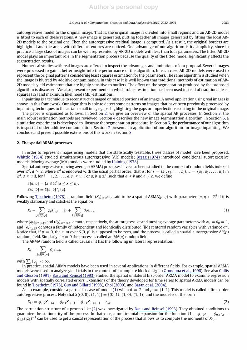
Fig. 1. (a) Original image; (b) Image generated by an AR-2D model; (c) Residual autoregressive image yielded by Algorithm 2.

Then the approximated image Z of the original image Z is

Zm,n = Xm,n + Z, 0 ≤ m ≤ M ′ − 1, 0 ≤ n ≤ N ′ − 1.

Nowwe describe the segmentation algorithm based on a generated image from Algorithm 1. Assume that an original imageZ is available.

Algorithm 2 (Segmentation Algorithm).

1. Use Algorithm 1 to generate an approximated image Z of Z .2. Compute the residual autoregressive image Z − Z .

Notice from step 2 in Algorithm 1 that the least squares estimators for the parameters of the AR-2D process have been used.However, Algorithm 2 is not necessarily dependent on this estimation method. Eventually, other estimation methods thatare able to reproduce well the homogeneous parts of the image, highlighting the borders and boundaries, could be used togenerated the fitted image. In particular, robust methods of estimation will be used in the next section when the originalimage is contaminated.

5. Numerical experiments

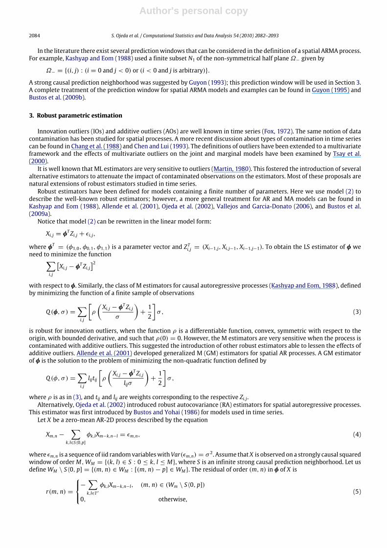
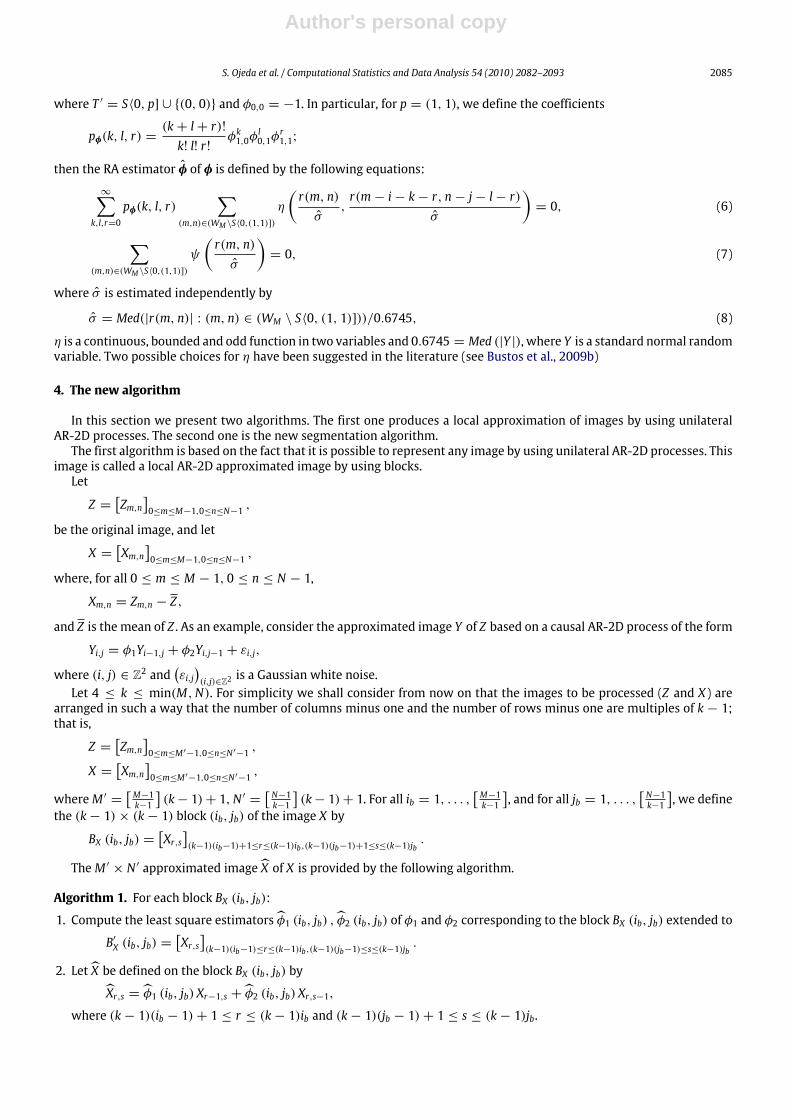
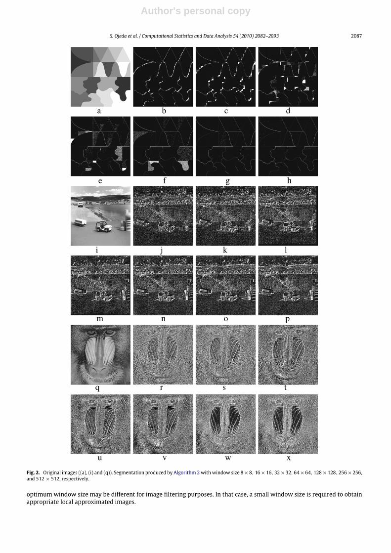
In this section, we present numerical experiments that illustrate the performance of Algorithm 2. The images consideredin the experiment were taken from the USC-SIPI image database http://sipi.usc.edu/database/. Fig. 1(a) shows an originalimage of size 512×512. Fig. 1(b) shows the image produced by Algorithm 1 using amovingwindow of size 7×7. In Fig. 1(c),we display the residual autoregressive image yielded byAlgorithm2. Notice fromFig. 1(b) that the local approximated imageis visually very similar to the original one. This is an interesting feature of the AR-2D model. A wide class of images can bewell represented by the images generated by Algorithm 1 in which the AR-2D model is fitted to 7 × 7 blocks and then thewhole original image is reproduced by putting all generated local images together. This form of image filtering based on theestimation of spatial autoregressivemodels has recently been studied by Bustos et al. (2009b). Themean square error (MSE)has been used to quantify the difference between the original and final images. In practice, the fitted spatial autoregressivemodel works well for a large class of images. However, Algorithm 1 does not work well, producing a large MSE for imagesaffected by a strong multiplicative speckle noise.In Figs. 2 and 3, four images (texmos, auto, mandrill, and Lenna) of size 512× 512 have been considered. These images

were processed by Algorithm 2with different moving window sizes. Images (b)–(h) were produced using amoving windowsize of 8×8, 16×16, 32×32, 64×64, 128×128, 256×256, and 512×512, respectively.We observe that the segmentationyielded by the proposed method strongly depends on the size of the moving window. The residual autoregressive imagesgeneratedwith a small window size seems to highlight the borders less than the images generatedwith a largewindow size.Moreover, the best performance is obtainedwhen using amovingwindow size of 512×512. That is, the fitted autoregressiveimage was generated using only one model. The same pattern is observed in all processed images. One possible reasonto explain this behavior is that a small window size is associated to a large number of AR models fitted to the originalimage. This produces a better local approximation, and hence the patterns in the fitted image are very well represented. Theresidual autoregressive image will not highlight the original borders and boundaries because both images are too similar.However, when the window size is large, the fitted image is a poor representation of the original patterns; thus the residualautoregressive image captures the large deviations from the original textures that are located at the borders or those areasthat divide the original image in several regions which usually show a variety of different textures. As a result, and basedon our experience dealing with Algorithm 2, we recommend using the maximum possible size for the moving window. This

Author's personal copy

S. Ojeda et al. / Computational Statistics and Data Analysis 54 (2010) 2082–2093 2087

a b c d

i j k l

m n o p

q r s t

u v w x

e f g h

Fig. 2. Original images ((a), (i) and (q)). Segmentation produced by Algorithm 2with window size 8×8, 16×16, 32×32, 64×64, 128×128, 256×256,and 512× 512, respectively.

optimum window size may be different for image filtering purposes. In that case, a small window size is required to obtainappropriate local approximated images.

Author's personal copy

2088 S. Ojeda et al. / Computational Statistics and Data Analysis 54 (2010) 2082–2093

a b c d

e f g h

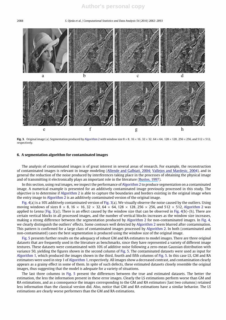
Fig. 3. Original image (a). Segmentation produced by Algorithm 2withwindow size 8×8, 16×16, 32×32, 64×64, 128×128, 256×256, and 512×512,respectively.

6. A segmentation algorithm for contaminated images

The analysis of contaminated images is of great interest in several areas of research. For example, the reconstructionof contaminated images is relevant in image modeling (Allende and Galbiati, 2004; Vallejos and Mardesic, 2004), and ingeneral the reduction of the noise produced by interferences taking place in the processes of obtaining the physical imageand of transmitting it electronically plays an important role in the literature (Bustos, 1997).In this section, using real images, we inspect the performance of Algorithm 2 to produce segmentation on a contaminated

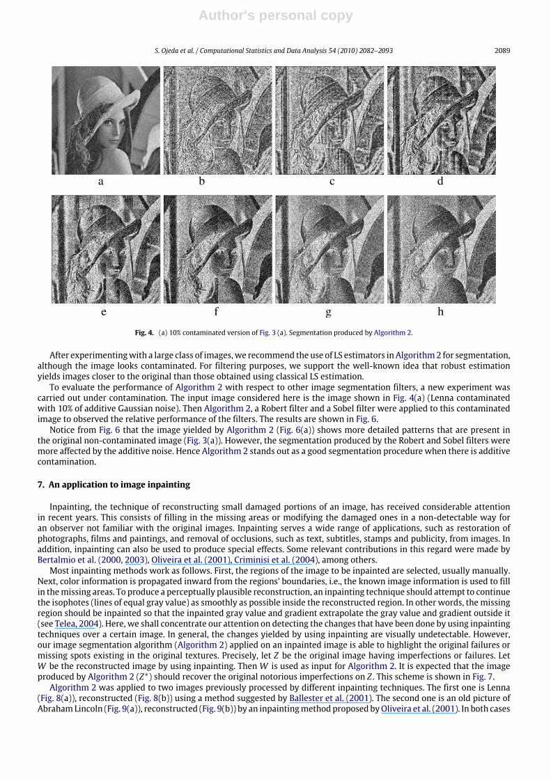
image. A numerical example is presented for an additively contaminated image previously processed in this study. Theobjective is to determine if Algorithm 2 is able to capture the boundaries and borders existing in the original image whenthe entry image to Algorithm 2 is an additively contaminated version of the original image.Fig. 4(a) is a 10% additively contaminated version of Fig. 3(a). We visually observe the noise caused by the outliers. Using

moving windows of sizes 8 × 8, 16 × 16, 32 × 32, 64 × 64, 128 × 128, 256 × 256, and 512 × 512, Algorithm 2 wasapplied to Lenna (Fig. 3(a)). There is an effect caused by the window size that can be observed in Fig. 4(b)–(h). There arecertain vertical blocks in all processed images, and the number of vertical blocks increases as the window size increases,making a strong difference between the segmentation produced by Algorithm 2 for non-contaminated images. In Fig. 4,we clearly distinguish the outliers’ effects. Some contours well detected by Algorithm 2 seem blurred after contamination.This pattern is confirmed for a large class of contaminated images processed by Algorithm 2. In both (contaminated andnon-contaminated) cases the best segmentation is produced using the window size of the original image.Fig. 5 presents further results on the adequacy of robust GM and RA estimates to model images. There are three original

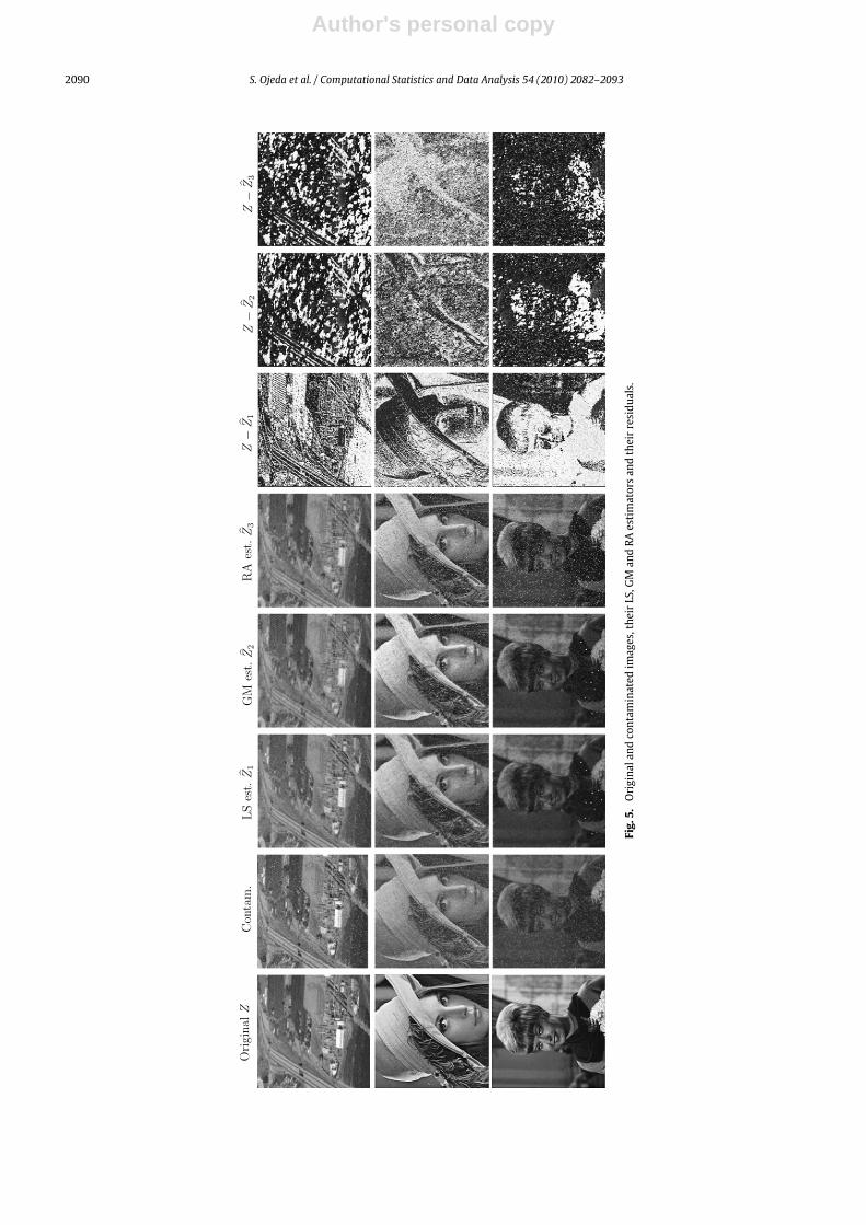
datasets that are frequently used in the literature as benchmarks, since they have represented a variety of different imagetextures. These datasets were contaminated with 10% of additive noise following a zero-mean Gaussian distribution withvariance 50, yielding the figures shown in the second column of Fig. 5. The contaminated datasets were used as input forAlgorithm 1, which produced the images shown in the third, fourth and fifth columns of Fig. 5. In this case LS, GM and RAestimators were used in step 1 of Algorithm 1, respectively. All images show a decreased contrast, and contamination clearlyappears as a grainy effect in some of them. In spite of such defects, these estimated datasets closely resemble the originalimages, thus suggesting that the model is adequate for a variety of situations.The last three columns in Fig. 5 present the differences between the true and estimated datasets. The better the

estimation, the less the information present in these error images. Clearly the LS estimations perform worse than GM andRA estimations, and as a consequence the images corresponding to the GM and RA estimators (last two columns) retainedless information than the classical version did. Also, notice that GM and RA estimations have a similar behavior. The LSestimations are clearly worse performers than the GM and RA estimations.

Author's personal copy

S. Ojeda et al. / Computational Statistics and Data Analysis 54 (2010) 2082–2093 2089

a b c d

e f g h

Fig. 4. (a) 10% contaminated version of Fig. 3 (a). Segmentation produced by Algorithm 2.

After experimentingwith a large class of images,we recommend the use of LS estimators in Algorithm2 for segmentation,although the image looks contaminated. For filtering purposes, we support the well-known idea that robust estimationyields images closer to the original than those obtained using classical LS estimation.To evaluate the performance of Algorithm 2 with respect to other image segmentation filters, a new experiment was

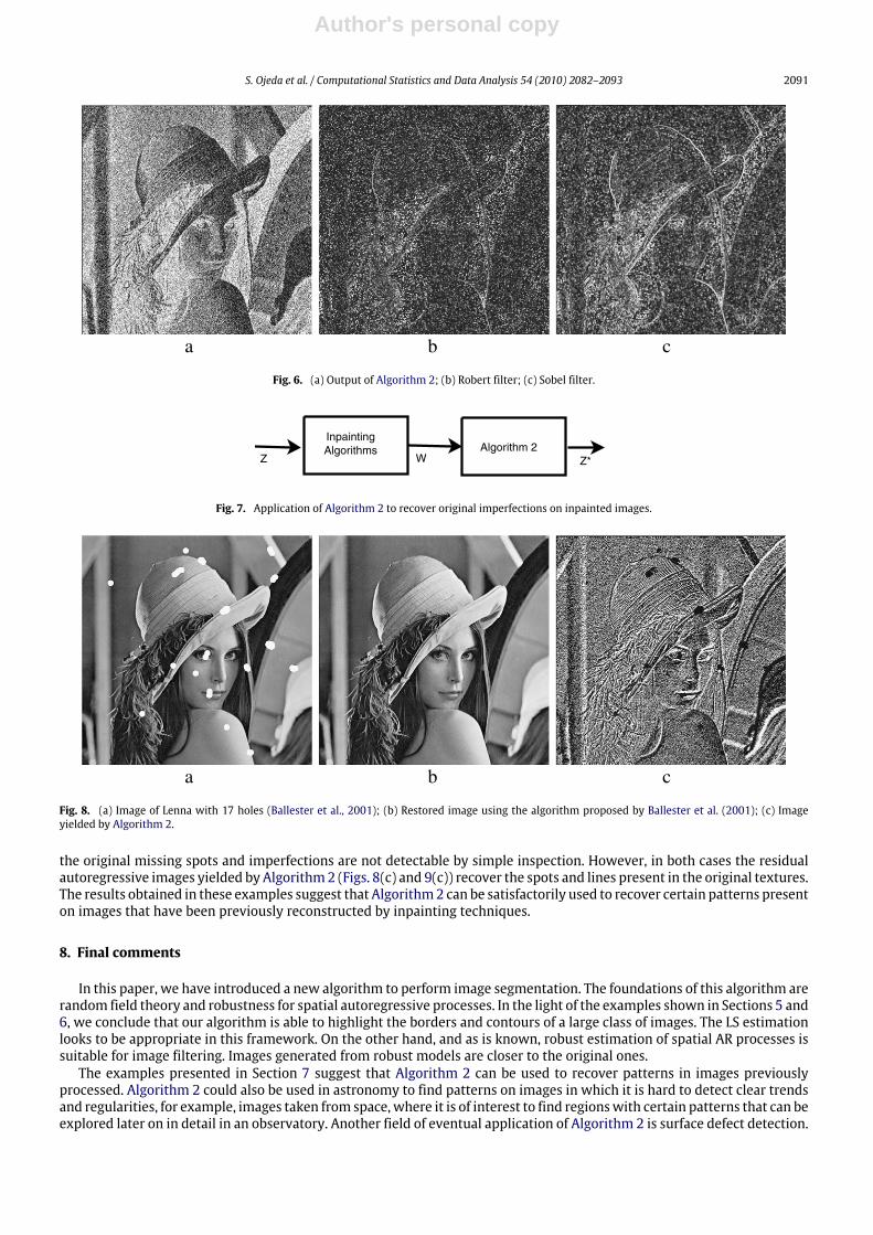
carried out under contamination. The input image considered here is the image shown in Fig. 4(a) (Lenna contaminatedwith 10% of additive Gaussian noise). Then Algorithm 2, a Robert filter and a Sobel filter were applied to this contaminatedimage to observed the relative performance of the filters. The results are shown in Fig. 6.Notice from Fig. 6 that the image yielded by Algorithm 2 (Fig. 6(a)) shows more detailed patterns that are present in

the original non-contaminated image (Fig. 3(a)). However, the segmentation produced by the Robert and Sobel filters weremore affected by the additive noise. Hence Algorithm 2 stands out as a good segmentation procedure when there is additivecontamination.

7. An application to image inpainting

Inpainting, the technique of reconstructing small damaged portions of an image, has received considerable attentionin recent years. This consists of filling in the missing areas or modifying the damaged ones in a non-detectable way foran observer not familiar with the original images. Inpainting serves a wide range of applications, such as restoration ofphotographs, films and paintings, and removal of occlusions, such as text, subtitles, stamps and publicity, from images. Inaddition, inpainting can also be used to produce special effects. Some relevant contributions in this regard were made byBertalmio et al. (2000, 2003), Oliveira et al. (2001), Criminisi et al. (2004), among others.Most inpainting methods work as follows. First, the regions of the image to be inpainted are selected, usually manually.

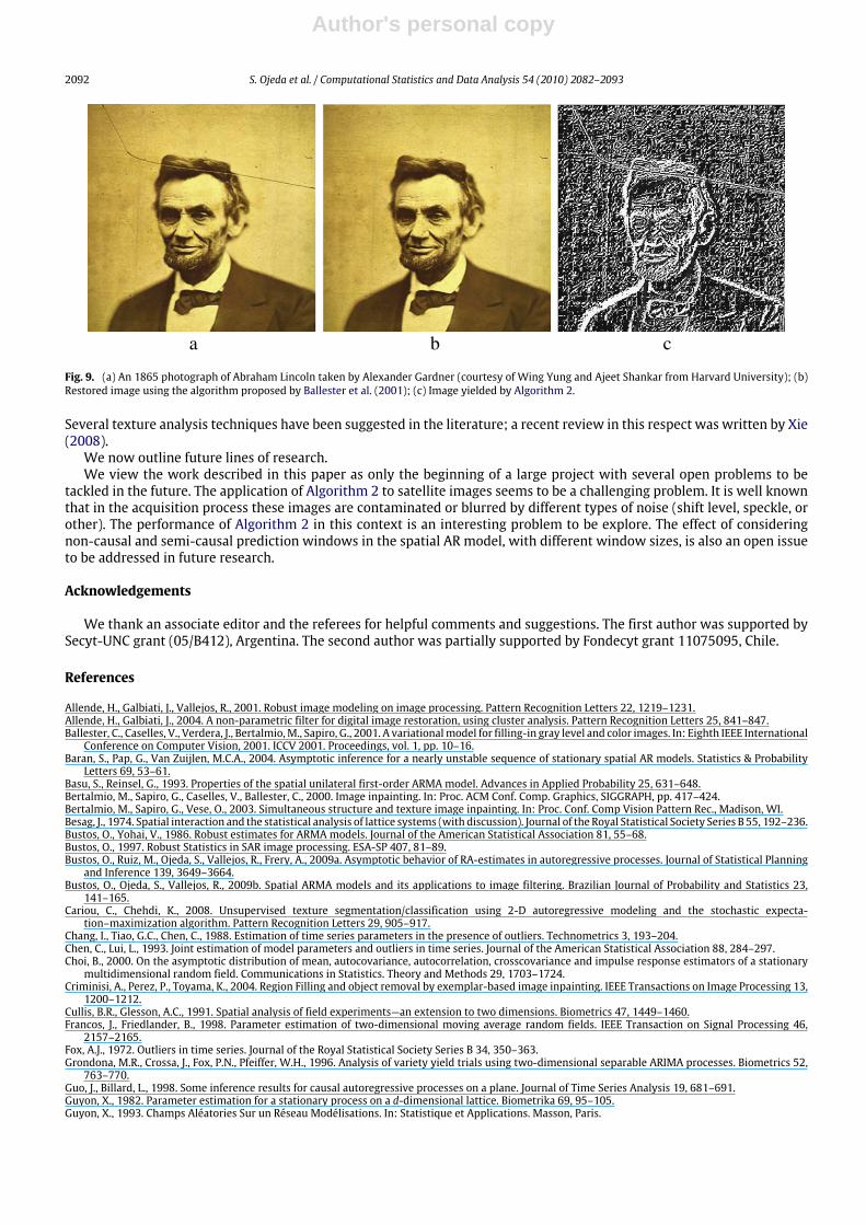
Next, color information is propagated inward from the regions’ boundaries, i.e., the known image information is used to fillin themissing areas. To produce a perceptually plausible reconstruction, an inpainting technique should attempt to continuethe isophotes (lines of equal gray value) as smoothly as possible inside the reconstructed region. In other words, themissingregion should be inpainted so that the inpainted gray value and gradient extrapolate the gray value and gradient outside it(see Telea, 2004). Here, we shall concentrate our attention on detecting the changes that have been done by using inpaintingtechniques over a certain image. In general, the changes yielded by using inpainting are visually undetectable. However,our image segmentation algorithm (Algorithm 2) applied on an inpainted image is able to highlight the original failures ormissing spots existing in the original textures. Precisely, let Z be the original image having imperfections or failures. LetW be the reconstructed image by using inpainting. ThenW is used as input for Algorithm 2. It is expected that the imageproduced by Algorithm 2 (Z∗) should recover the original notorious imperfections on Z . This scheme is shown in Fig. 7.Algorithm 2 was applied to two images previously processed by different inpainting techniques. The first one is Lenna

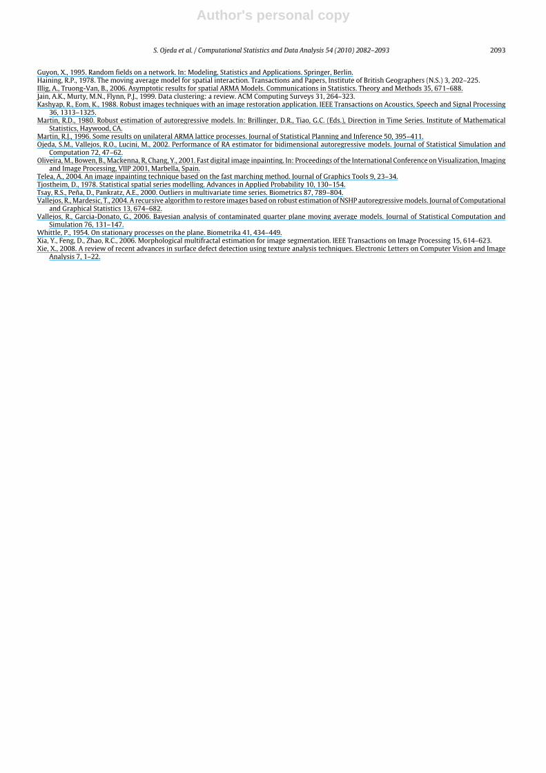
(Fig. 8(a)), reconstructed (Fig. 8(b)) using a method suggested by Ballester et al. (2001). The second one is an old picture ofAbrahamLincoln (Fig. 9(a)), reconstructed (Fig. 9(b)) by an inpaintingmethodproposed byOliveira et al. (2001). In both cases

Author's personal copy

2090 S. Ojeda et al. / Computational Statistics and Data Analysis 54 (2010) 2082–2093

Fig.

5.Originalandcontaminatedimages,theirLS,GMandRAestimatorsandtheirresiduals.

Author's personal copy

S. Ojeda et al. / Computational Statistics and Data Analysis 54 (2010) 2082–2093 2091

a b c

Fig. 6. (a) Output of Algorithm 2; (b) Robert filter; (c) Sobel filter.

InpaintingAlgorithms Algorithm 2

WZ Z*

Fig. 7. Application of Algorithm 2 to recover original imperfections on inpainted images.

a b c

Fig. 8. (a) Image of Lenna with 17 holes (Ballester et al., 2001); (b) Restored image using the algorithm proposed by Ballester et al. (2001); (c) Imageyielded by Algorithm 2.

the original missing spots and imperfections are not detectable by simple inspection. However, in both cases the residualautoregressive images yielded by Algorithm2 (Figs. 8(c) and 9(c)) recover the spots and lines present in the original textures.The results obtained in these examples suggest that Algorithm2 can be satisfactorily used to recover certain patterns presenton images that have been previously reconstructed by inpainting techniques.

8. Final comments

In this paper, we have introduced a new algorithm to perform image segmentation. The foundations of this algorithm arerandom field theory and robustness for spatial autoregressive processes. In the light of the examples shown in Sections 5 and6, we conclude that our algorithm is able to highlight the borders and contours of a large class of images. The LS estimationlooks to be appropriate in this framework. On the other hand, and as is known, robust estimation of spatial AR processes issuitable for image filtering. Images generated from robust models are closer to the original ones.The examples presented in Section 7 suggest that Algorithm 2 can be used to recover patterns in images previously

processed. Algorithm 2 could also be used in astronomy to find patterns on images in which it is hard to detect clear trendsand regularities, for example, images taken from space, where it is of interest to find regionswith certain patterns that can beexplored later on in detail in an observatory. Another field of eventual application of Algorithm 2 is surface defect detection.

Author's personal copy

2092 S. Ojeda et al. / Computational Statistics and Data Analysis 54 (2010) 2082–2093

a b c

Fig. 9. (a) An 1865 photograph of Abraham Lincoln taken by Alexander Gardner (courtesy of Wing Yung and Ajeet Shankar from Harvard University); (b)Restored image using the algorithm proposed by Ballester et al. (2001); (c) Image yielded by Algorithm 2.

Several texture analysis techniques have been suggested in the literature; a recent review in this respect was written by Xie(2008).We now outline future lines of research.We view the work described in this paper as only the beginning of a large project with several open problems to be

tackled in the future. The application of Algorithm 2 to satellite images seems to be a challenging problem. It is well knownthat in the acquisition process these images are contaminated or blurred by different types of noise (shift level, speckle, orother). The performance of Algorithm 2 in this context is an interesting problem to be explore. The effect of consideringnon-causal and semi-causal prediction windows in the spatial AR model, with different window sizes, is also an open issueto be addressed in future research.

Acknowledgements

We thank an associate editor and the referees for helpful comments and suggestions. The first author was supported bySecyt-UNC grant (05/B412), Argentina. The second author was partially supported by Fondecyt grant 11075095, Chile.

References

Allende, H., Galbiati, J., Vallejos, R., 2001. Robust image modeling on image processing. Pattern Recognition Letters 22, 1219–1231.Allende, H., Galbiati, J., 2004. A non-parametric filter for digital image restoration, using cluster analysis. Pattern Recognition Letters 25, 841–847.Ballester, C., Caselles, V., Verdera, J., Bertalmio,M., Sapiro, G., 2001. A variationalmodel for filling-in gray level and color images. In: Eighth IEEE InternationalConference on Computer Vision, 2001. ICCV 2001. Proceedings, vol. 1, pp. 10–16.

Baran, S., Pap, G., Van Zuijlen, M.C.A., 2004. Asymptotic inference for a nearly unstable sequence of stationary spatial AR models. Statistics & ProbabilityLetters 69, 53–61.

Basu, S., Reinsel, G., 1993. Properties of the spatial unilateral first-order ARMA model. Advances in Applied Probability 25, 631–648.Bertalmio, M., Sapiro, G., Caselles, V., Ballester, C., 2000. Image inpainting. In: Proc. ACM Conf. Comp. Graphics, SIGGRAPH, pp. 417–424.Bertalmio, M., Sapiro, G., Vese, O., 2003. Simultaneous structure and texture image inpainting. In: Proc. Conf. Comp Vision Pattern Rec., Madison, WI.Besag, J., 1974. Spatial interaction and the statistical analysis of lattice systems (with discussion). Journal of the Royal Statistical Society Series B 55, 192–236.Bustos, O., Yohai, V., 1986. Robust estimates for ARMA models. Journal of the American Statistical Association 81, 55–68.Bustos, O., 1997. Robust Statistics in SAR image processing. ESA-SP 407, 81–89.Bustos, O., Ruiz, M., Ojeda, S., Vallejos, R., Frery, A., 2009a. Asymptotic behavior of RA-estimates in autoregressive processes. Journal of Statistical Planningand Inference 139, 3649–3664.

Bustos, O., Ojeda, S., Vallejos, R., 2009b. Spatial ARMA models and its applications to image filtering. Brazilian Journal of Probability and Statistics 23,141–165.

Cariou, C., Chehdi, K., 2008. Unsupervised texture segmentation/classification using 2-D autoregressive modeling and the stochastic expecta-tion–maximization algorithm. Pattern Recognition Letters 29, 905–917.

Chang, I., Tiao, G.C., Chen, C., 1988. Estimation of time series parameters in the presence of outliers. Technometrics 3, 193–204.Chen, C., Lui, L., 1993. Joint estimation of model parameters and outliers in time series. Journal of the American Statistical Association 88, 284–297.Choi, B., 2000. On the asymptotic distribution of mean, autocovariance, autocorrelation, crosscovariance and impulse response estimators of a stationarymultidimensional random field. Communications in Statistics. Theory and Methods 29, 1703–1724.

Criminisi, A., Perez, P., Toyama, K., 2004. Region Filling and object removal by exemplar-based image inpainting. IEEE Transactions on Image Processing 13,1200–1212.

Cullis, B.R., Glesson, A.C., 1991. Spatial analysis of field experiments—an extension to two dimensions. Biometrics 47, 1449–1460.Francos, J., Friedlander, B., 1998. Parameter estimation of two-dimensional moving average random fields. IEEE Transaction on Signal Processing 46,2157–2165.

Fox, A.J., 1972. Outliers in time series. Journal of the Royal Statistical Society Series B 34, 350–363.Grondona, M.R., Crossa, J., Fox, P.N., Pfeiffer, W.H., 1996. Analysis of variety yield trials using two-dimensional separable ARIMA processes. Biometrics 52,763–770.

Guo, J., Billard, L., 1998. Some inference results for causal autoregressive processes on a plane. Journal of Time Series Analysis 19, 681–691.Guyon, X., 1982. Parameter estimation for a stationary process on a d-dimensional lattice. Biometrika 69, 95–105.Guyon, X., 1993. Champs Aléatories Sur un Réseau Modélisations. In: Statistique et Applications. Masson, Paris.

Author's personal copy

S. Ojeda et al. / Computational Statistics and Data Analysis 54 (2010) 2082–2093 2093

Guyon, X., 1995. Random fields on a network. In: Modeling, Statistics and Applications. Springer, Berlin.Haining, R.P., 1978. The moving average model for spatial interaction. Transactions and Papers, Institute of British Geographers (N.S.) 3, 202–225.Illig, A., Truong-Van, B., 2006. Asymptotic results for spatial ARMA Models. Communications in Statistics. Theory and Methods 35, 671–688.Jain, A.K., Murty, M.N., Flynn, P.J., 1999. Data clustering: a review. ACM Computing Surveys 31, 264–323.Kashyap, R., Eom, K., 1988. Robust images techniques with an image restoration application. IEEE Transactions on Acoustics, Speech and Signal Processing36, 1313–1325.

Martin, R.D., 1980. Robust estimation of autoregressive models. In: Brillinger, D.R., Tiao, G.C. (Eds.), Direction in Time Series. Institute of MathematicalStatistics, Haywood, CA.

Martin, R.J., 1996. Some results on unilateral ARMA lattice processes. Journal of Statistical Planning and Inference 50, 395–411.Ojeda, S.M., Vallejos, R.O., Lucini, M., 2002. Performance of RA estimator for bidimensional autoregressive models. Journal of Statistical Simulation andComputation 72, 47–62.

Oliveira,M., Bowen, B.,Mackenna, R, Chang, Y., 2001. Fast digital image inpainting. In: Proceedings of the International Conference onVisualization, Imagingand Image Processing, VIIP 2001, Marbella, Spain.

Telea, A., 2004. An image inpainting technique based on the fast marching method. Journal of Graphics Tools 9, 23–34.Tjostheim, D., 1978. Statistical spatial series modelling. Advances in Applied Probability 10, 130–154.Tsay, R.S., Peña, D., Pankratz, A.E., 2000. Outliers in multivariate time series. Biometrics 87, 789–804.Vallejos, R.,Mardesic, T., 2004. A recursive algorithm to restore images based on robust estimation of NSHP autoregressivemodels. Journal of Computationaland Graphical Statistics 13, 674–682.

Vallejos, R., Garcia-Donato, G., 2006. Bayesian analysis of contaminated quarter plane moving average models. Journal of Statistical Computation andSimulation 76, 131–147.

Whittle, P., 1954. On stationary processes on the plane. Biometrika 41, 434–449.Xia, Y., Feng, D., Zhao, R.C., 2006. Morphological multifractal estimation for image segmentation. IEEE Transactions on Image Processing 15, 614–623.Xie, X., 2008. A review of recent advances in surface defect detection using texture analysis techniques. Electronic Letters on Computer Vision and ImageAnalysis 7, 1–22.