A new hybrid artificial neural networks and fuzzy regression model for time series forecasting

Fuzzy Sets and Systems 159 (2008) 769–786www.elsevier.com/locate/fss

A new hybrid artificial neural networks and fuzzy regression modelfor time series forecasting

Mehdi Khashei, Seyed Reza Hejazi∗, Mehdi BijariDepartment of Industrial Engineering, Isfahan University of Technology, Isfahan 84156-83111, Iran

Received 20 November 2006; received in revised form 20 August 2007; accepted 16 October 2007Available online 30 October 2007

Abstract

Quantitative methods have nowadays become very important tools for forecasting purposes in financial markets as for improveddecisions and investments. Forecasting accuracy is one of the most important factors involved in selecting a forecasting method;hence, never has research directed at improving upon the effectiveness of time series models stopped. Artificial neural networks(ANNs) are flexible computing frameworks and universal approximators that can be applied to a wide range of forecasting problemswith a high degree of accuracy. However, ANNs need a large amount of historical data in order to yield accurate results. In areal world situation and in financial markets specifically, the environment is full of uncertainties and changes occur rapidly; thus,future situations must be usually forecasted using the scant data made available over a short span of time. Therefore, forecasting inthese situations requires methods that work efficiently with incomplete data. Although fuzzy forecasting methods are suitable forincomplete data situations, their performance is not always satisfactory. In this paper, based on the basic concepts of ANNs and fuzzyregression models, a new hybrid method is proposed that yields more accurate results with incomplete data sets. In our proposedmodel, the advantages of ANNs and fuzzy regression are combined to overcome the limitations in both ANNs and fuzzy regressionmodels. The empirical results of financial market forecasting indicate that the proposed model can be an effective way of improvingforecasting accuracy.© 2007 Elsevier B.V. All rights reserved.

Keywords: Artificial neural networks (ANNs); Fuzzy regression; Fuzzy time series; Hybrid models; Financial markets forecasting

1. Introduction

In today’s world, quantitative methods are crucial for forecast purposes in financial markets as well as for improveddecisions and investments. Recently, artificial neural networks (ANNs) have been extensively studied and used intime-series forecasting. Zhang et al. [68] presented a recent review of the efforts in this area. The major advantage ofneural networks is their flexible nonlinear modeling capability. With ANNs, there is no need to specify a particularmodel form. Rather, the model is adaptively formed based on the features presented in the data. This data-drivenapproach is suitable for many empirical data sets where no theoretical guidance is available to suggest an appropriatedata generating process. Despite the advantages cited for them, ANNs have weaknesses, one of the most important ofwhich is their requirement for large amounts of data in order to yield accurate results [32].

No definite rule exists for the sample size requirement of a given problem. The amount of data for network trainingdepends on the network structure, the training method, and the complexity of the particular problem or the amount of

∗ Corresponding author. Tel.: +98 311 3912550x1; fax: +98 311 3915526.E-mail address: [email protected] (S.R. Hejazi).

0165-0114/$ - see front matter © 2007 Elsevier B.V. All rights reserved.doi:10.1016/j.fss.2007.10.011

http://www.elsevier.com/locate/fss

mailto:[email protected]

770 M. Khashei et al. / Fuzzy Sets and Systems 159 (2008) 769–786

noise in the data on hand. Nam and Schaefer [42] tested the effect of different training sample sizes and found that asthe training sample size increased, the ANN forecaster performed better. With a large enough sample, ANNs can modelany complex structure in the data. Hence, ANNs can benefit more from large samples than linear statistical models can.It is interesting to note that ANNs do not necessarily require a larger sample than is required by linear models in orderto perform well. Kang [31] found that ANN forecasting models perform quite well even with sample sizes smaller than50, while the Box–Jenkins models typically require at least 50 data points in order to forecast successfully [7].

Fuzzy forecasting methods are suitable under incomplete data conditions and require fewer observations than otherforecasting models, but their performance is not always satisfactory. Fuzzy theory was originally developed to deal withproblems involving linguistic terms [65–67] and have been successfully applied to various applications such as universityenrollment forecasting [10,11,14,15,23,53], financial forecasting [24,25,64,21,60,35], temperature forecasting [15],reactors [59], etc. Tanaka et al. [54–56] have suggested fuzzy regression to solve the fuzzy environment and to avoid amodeling error. This model is basically an interval prediction model with the disadvantage that the prediction intervalcan be very wide if some extreme values are present. Watada [61] found an application of fuzzy regression to fuzzytime-series analysis.

Time-series models had failed to consider the application of fuzzy theory until Song and Chissom [50,52] definedfuzzy time-series. They proposed the definitions of fuzzy time-series and methods to model fuzzy relationships amongobservations. Different fuzzy time-series models have been proposed by following Song and Chissom’s definitionof fuzzy time-series [51]. For example, there have been Song and Chissom’s time-invariant model [50], Song andChissom’s time-variant model [52], the Markov model [53], Chen’s model [11], Hwang’s model [27], the seasonalmodel [9,49], the heuristic model [23], the high order model [12], the nth order heuristic model [24], etc.

In the evolution of fuzzy time-series models, Chen [11] proposed another method to apply simplified arithmeticoperations in forecasting algorithms rather than the complicated maximum–minimum composition operations presentedin Song and Chissom’s models. In subsequent research, Chen also proposed several methods, such as high-order fuzzyrelationships [14,12,13,27]. Additionally, Huarng [22] pointed out that the length of intervals affected the forecastingaccuracy in fuzzy time-series and proposed a method with distribution-based and average-based lengths to reconcilethis issue. In Huarng’s model, two different lengths of intervals were applied to Chen’s model and it was concluded thatdistribution-based and average-based lengths could improve forecasting accuracy [22]. Yu [63] proposed a weightedmodel to tackle two issues, recurrence and weighting, in fuzzy time-series forecasting and concluded that the weightedmodel outperforms one of the conventional fuzzy time-series models. Other similar work on fuzzy time-series can befound in [41].

Using hybrid models or combining several models has become a common practice to improve forecasting accuracy.The literature on this topic has expanded dramatically since the early work of Reid [46] and Bates and Granger[4]. Clemen provided a comprehensive review and annotated bibliography in this area [16]. The basic idea of themodel combination in forecasting is to use each model’s unique feature to capture different patterns in the data. Boththeoretical and empirical findings suggest that combining different methods can be an effective and efficient way toimprove forecasts [2,37]. Tseng et al. proposed a Fuzzy auto regressive integrated moving average (FARIMA) methodto use the advantages and to fulfill the limitations of the fuzzy regression and auto regressive integrated moving average(ARIMA) models for time-series forecasting [58]. Genetic algorithms and neural networks are usually proposed forimproving the forecasting accuracy of fuzzy time-series models. Chen et al. [13] presented a hybrid genetic algorithmand a high-order fuzzy time-series approach for enrollment forecasting. Huarng et al. [26] described a combiningmethodology using neural networks to forecast fuzzy time-series.

In this paper, a new hybrid model is proposed based on the basic concepts of ANNs and fuzzy regression modelsapproaches to time-series forecasting under incomplete data conditions. In the proposed model, the ANN is usedto preprocess raw data and to provide the necessary background to apply a fuzzy regression model. To show itsappropriateness and effectiveness, our proposed method is applied to financial markets forecasting problems and theirperformance is compared with those of other forecasting models such as auto regressive integrated moving average,Chen’s fuzzy time-series (first and high-order) [11,13],Yu’s fuzzy time-series [63], FARIMA [58], andANNs. Empiricalresults of two cases of exchange rate and gold price forecasting indicate that the proposed model is an effective methodto improve forecasting accuracy.

The paper is organized as follows: The ANN modeling approaches to time-series forecasting are reviewed inSection 2. Basic concepts of fuzzy regression and fuzzy time-series are explained in Section 3. In Section 4, theproposed model is formulated. In Section 5, the proposed model is applied to financial markets forecasting and its

M. Khashei et al. / Fuzzy Sets and Systems 159 (2008) 769–786 771

performance is compared to other forecasting models in exchange rate and precious metals forecasting cases. Finally,comes a section on conclusions.

2. The ANN approach to time-series modeling

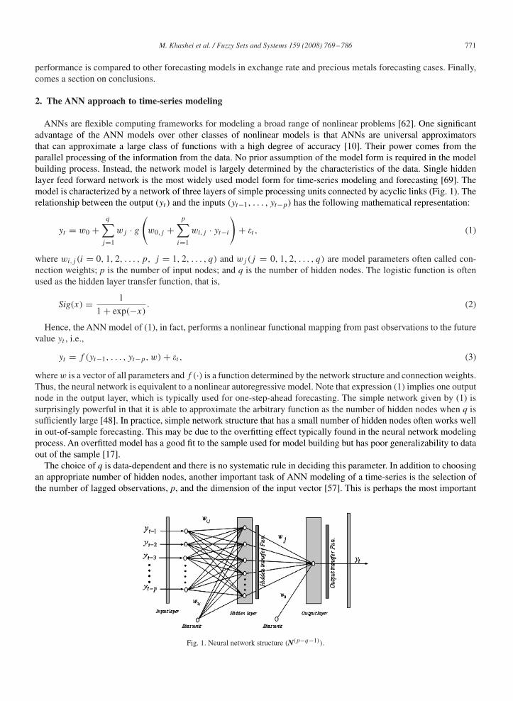
ANNs are flexible computing frameworks for modeling a broad range of nonlinear problems [62]. One significantadvantage of the ANN models over other classes of nonlinear models is that ANNs are universal approximatorsthat can approximate a large class of functions with a high degree of accuracy [10]. Their power comes from theparallel processing of the information from the data. No prior assumption of the model form is required in the modelbuilding process. Instead, the network model is largely determined by the characteristics of the data. Single hiddenlayer feed forward network is the most widely used model form for time-series modeling and forecasting [69]. Themodel is characterized by a network of three layers of simple processing units connected by acyclic links (Fig. 1). Therelationship between the output (yt ) and the inputs (yt−1, . . . , yt−p) has the following mathematical representation:

yt = w0 +q∑

j=1

wj · g

(w0,j +

p∑i=1

wi,j · yt−i

)+ �t , (1)

where wi,j (i = 0, 1, 2, . . . , p, j = 1, 2, . . . , q) and wj(j = 0, 1, 2, . . . , q) are model parameters often called con-nection weights; p is the number of input nodes; and q is the number of hidden nodes. The logistic function is oftenused as the hidden layer transfer function, that is,

Sig(x) = 1

1 + exp(−x). (2)

Hence, the ANN model of (1), in fact, performs a nonlinear functional mapping from past observations to the futurevalue yt , i.e.,

yt = f (yt−1, . . . , yt−p, w) + �t , (3)

where w is a vector of all parameters and f (·) is a function determined by the network structure and connection weights.Thus, the neural network is equivalent to a nonlinear autoregressive model. Note that expression (1) implies one outputnode in the output layer, which is typically used for one-step-ahead forecasting. The simple network given by (1) issurprisingly powerful in that it is able to approximate the arbitrary function as the number of hidden nodes when q issufficiently large [48]. In practice, simple network structure that has a small number of hidden nodes often works wellin out-of-sample forecasting. This may be due to the overfitting effect typically found in the neural network modelingprocess. An overfitted model has a good fit to the sample used for model building but has poor generalizability to dataout of the sample [17].

The choice of q is data-dependent and there is no systematic rule in deciding this parameter. In addition to choosingan appropriate number of hidden nodes, another important task of ANN modeling of a time-series is the selection ofthe number of lagged observations, p, and the dimension of the input vector [57]. This is perhaps the most important

Fig. 1. Neural network structure (N(p−q−1)).


parameter to be estimated in an ANN model because it plays a major role in determining the (nonlinear) autocorrelationstructure of the time-series.

There exist many different approaches such as the pruning algorithm, the polynomial time algorithm, the canonicaldecomposition technique, and the network information criterion for finding the optimal architecture of an ANN [32].These approaches can be generally categorized as follows: (i) Empirical or statistical methods that are used to studythe effect of an ANN’s internal parameters and choose appropriate values for them based on the model’s performance[6,38]. The most systematic and general of these methods utilizes the principles from Taguchi’s design of experiments[47]. (ii) Hybrid methods such as fuzzy inference [36] where the ANN can be interpreted as an adaptive fuzzy systemor it can operate on fuzzy instead of real numbers. (iii) Constructive and/or pruning algorithms that, respectively,add and/or remove neurons from an initial architecture using a previously specified criterion to indicate how ANNperformance is affected by the changes [3,29,30,38]. The basic rules are that neurons are added when training is slow orwhen the mean squared error is larger than a specified value, and that neurons are removed when a change in a neuron’svalue does not correspond to a change in the network’s response or when the weight values that are associated withthis neuron remain constant for a large number of training epochs [40]. (iv). Evolutionary strategies that search overtopology space by varying the number of hidden layers and hidden neurons through application of genetic operators[8,34] and evaluation of the different architectures according to an objective function [1,6].

Although there exists many different approaches for finding the optimal architecture of an ANN, these methods areusually quite complex in nature and are difficult to implement [68]. Furthermore, none of these methods can guaranteethe optimal solution for all real forecasting problems. To date, there is no simple clear-cut method for determinationof these parameters and the usual procedure is to test numerous networks with varying numbers of input and hiddenunits (p, q), estimate generalization error for each, and select the network with the lowest generalization error [20].Once a network structure (p, q) is specified, the network is ready for training a process of parameter estimation. Theparameters are estimated such that an overall accuracy criterion such as the mean squared error is minimized. This isdone with some efficient nonlinear optimization algorithms other than the basic backpropagation training algorithm[43]. The estimated model is usually evaluated using a separate hold-out sample that is not exposed to the trainingprocess.

3. Fuzzy forecasting models

This section briefly reviews the fuzzy forecasting models, including fuzzy time-series and fuzzy regression models.

3.1. Fuzzy time-series

Since Zadeh [65–67] introduced the Fuzzy Set Theory, it provides a powerful framework to cope with vague orambiguous problems and can express linguistic values and human subjective judgments of natural language. Time-series models had failed to consider the application of this theory until fuzzy time-series was defined by Song andChissom [50,52]. In recent years, many fuzzy time-series models have been proposed following Song and Chissom’sdefinitions. Among these models, Chen’s model is a more conventional one because of its easy calculations and goodforecasting performance. Therefore, Song and Chissom’s definitions [50,52] and Chen’s algorithm [11] are used asillustrations below:

Definition 1 (Fuzzy time-series). Let Y (t) (. . . , 0, 1, 2, . . .), a subset of real numbers, be the universe of discourse bywhich fuzzy sets fj (t) are defined. If F(t) is a collection of f1(t), f2(t), . . . , then F(t) is called a fuzzy time-seriesdefined on Y (t).

Definition 2 (Fuzzy relation). If there exists a fuzzy logical relationship (FLR) R(t−1, t), such that F(t) = F(t − 1) o

R(t − 1, t), where “o” represents the max–min composition operator, F(t − 1) and F(t) are fuzzy sets, then F(t) is saidto be caused by F(t − 1). The logical relationship between F(t) and F(t − 1) can be represented as F(t − 1) → F(t).

Definition 3. Let F(t − 1) = Ai and F(t) = Aj . The relationship between two consecutive observations, F(t) andF(t − 1), referred to as a FLR, can be denoted by Ai → Aj , where Ai is called the left-hand side (LHS) and Aj theright-hand side (RHS) of the FLR.


Definition 4. All FCRs in the training dataset can be further grouped together into different FLR groups according tothe same left-hand sides of the FLR. For example, there are two FLRs with the same left-hand side (Ai) : Ai → Aj1and Ai → Aj2. These two FLRs can be grouped into a FLR group.

Definition 5 (Time-invariant fuzzy time-series and time-variant fuzzy time-series). SupposeF(t) is caused byF(t − 1)

only, and F(t) = F(t − 1) o R(t − 1, t). For any t , if R(t − 1, t) is independent of t, then F(t) is named a time-invariantfuzzy time-series, otherwise it is a time-variant fuzzy time-series.

3.1.1. The algorithm of Chen’s modelStep 1: (Define the universe of discourse and intervals for rules abstraction). Based on the issue domain, the universe

of discourse can be defined as: U = [starting ending]. As the length of interval is determined, U can be partitionedinto several equal length intervals.

Step 2: Define fuzzy sets based on the universe of discourse and fuzzify the historical data.Step 3: (Fuzzify observed rules). For example, a datum is fuzzified to Aj if the maximal degree of membership of

that datum is Aj .Step 4: Establish FLRs and group them based on the current states of the data of the FLRs. For example, A1 → A1,

A1 → A2, A1 → A3 can be grouped as: A1 → A1, A2, A3.Step 5: (Forecast). Let F(t − 1) = Ai . Case 1: There is only one FLR in the FLR sequence. If Ai → Aj , then F(t),

forecast value, is equal to Aj . Case 2: If Ai → Ai, Aj , . . . , Ak , then F(t), forecast value, is equal to Ai, Aj , . . . , Ak .Step 6: (Defuzzify). Apply “Centroid” method to get the results. This procedure (also called center of area, center of

gravity) is the most often adopted method of defuzzification.

3.2. Fuzzy regression models

Statistical models use the concept of measurement error to deal with the difference between estimators and observa-tions, but these data are precise values and do not include measurement errors. It is the same as the basic concept of thefuzzy regression model suggested by Tanaka et al. [55]. The basic concept of the fuzzy theory of fuzzy regression is thatthe residuals between estimators and observations are not produced by measusrement errors, rather by the parameteruncertainty in the model, and the possibility distribution is used to deal with real observations. The following is ageneralized model of fuzzy linear regression:

Y = �0 + �1x1 + · · · + �nxn =n∑

i=0

�ixi = x′�, (4)

where x is the vector of independent variables, superscript ′ denotes the transposition operation, n is the numberof variables, and �i represents fuzzy sets representing the ith parameter of the model. Instead of using crisp, fuzzyparameter �i in the form of L-type fuzzy numbers of Dubois and Prade [18], (�i , ci)L, the possibility distribution is

��i(�i ) = L{(�i − �i/c)}, (5)

where L is a function type. Fuzzy parameters in the form of triangular fuzzy numbers are used:

��i(�i ) =

⎧⎨⎩ 1 − |�i − �i |

ci

, �i − ci ��i ��i + ci,

0 otherwise,(6)

where ��i(�i ) the membership function of the fuzzy set is represented by parameter �i , �i is the center of the fuzzy

number, and ci is the width or spread around the center of the fuzzy number. Through the extension principle, themembership function of the fuzzy number yt = x′

t � can be defined using pyramidal fuzzy parameter � as follows:

�y (yt ) =

⎧⎪⎪⎨⎪⎪⎩

1 − |yt − xt�|c′|xt | for xt �= 0,

1 for xt = 0, yt = 0,

0 for xt = 0, yt �= 0,

(7)


where � and c denote vectors of model values and spreads, all model parameters, respectively; t is the number ofobservations, t = 1, 2, . . . , k. Finally, the method uses the criterion of minimizing total vagueness, S, defined as thesum of individual spreads of the fuzzy parameters of the model.

Minimize S =k∑

t=1

c′|xt |. (8)

At the same time, this approach takes into account the condition that the membership value of each observation yt isgreater than an imposed threshold, h level, h ∈ [0, 1]. This criterion data simply express the fact that the fuzzy output ofthe model should be over all the data points y1, y2, . . . , yk to a certain h-level. A choice of the h-level value influencesthe widths c of the fuzzy parameters:

�y (yt )�h for t = 1, 2, . . . , k. (9)

The index t refers to the number of nonfuzzy data used in constructing the model. The problem of finding the fuzzyregression parameters was formulated by Tanaka et al. [55] as a linear programming problem:

Minimize S =k∑

t=1

c′|xt |

subject to

⎧⎨⎩

x′t� + (1 − h)c′|xt |�yt , t = 1, 2, . . . , k,

x′t� − (1 − h)c′|xt |�yt , t = 1, 2, . . . , k,

c�0,

(10)

where �′ = (�1, �2, . . . , �n) and c′ = (c1, c2, . . . , cn) are vectors of unknown variables and S is the total vagueness aspreviously defined.

4. Formulation of the proposed model

The ANNs model is a precise forecasting model for a broad range of nonlinear problems, but it requires a largeamount of historical data to produce accurate results. However, in our society today, due to factors of uncertaintyfrom the integral environment and rapid development of new technologies, we usually have to forecast future sit-uations using little data over a short span of time. Therefore, we need forecasting methods that are efficient underincomplete data conditions. The fuzzy regression model is the suitable interval-forecasting model for cases whereinadequate historical data are available. The purpose of this paper is to use the advantages of the fuzzy regres-sion models to eliminate the limitation of a large amount of historical data imposed on formulating the proposedmodel.

The parameter of ANNs model (weights and biases) are crisp (wi,j (i = 0, 1, 2, . . . , p, j = 1, 2, . . . , q),wj(j = 0, 1, 2, . . . , q)). Instead of using crisp, fuzzy parameters in the form of triangular fuzzy numbers are usedfor related parameters of layers (wi,j (i = 0, 1, 2, . . . , p, j = 1, 2, . . . , q), wj (j = 0, 1, 2, . . . , q)). In addition, thisstudy adapts the methodology formulated by Ishibuchi and Tanaka [28] for the condition which includes a widespread of the forecasted interval. A proposed model is described using a fuzzy function with a fuzzyparameter:

yt = f

⎛⎝w0 +

q∑j=1

wj · g

(w0,j +

p∑i=1

wi,j · yt−i

)⎞⎠ , (11)

where yt are observations, wi,j (i = 0, 1, 2, . . . , p, j = 1, 2, . . . , q), wj (j = 0, 1, 2, . . . , q) are fuzzy numbers.Eq. (11) is modified as follows:

yt = f

⎛⎝w0 +

q∑j=1

wj · Xt,j

⎞⎠ = f

⎛⎝ q∑

j=0

wj · Xt,j

⎞⎠ , (12)


where Xt,j = g(w0,j + ∑pi=1 wi,j · yt−i ). Fuzzy parameters in the form of triangular fuzzy numbers wi,j =

(ai,j , bi,j , ci,j ) are used:

�wi,j(wi,j ) =

⎧⎪⎪⎪⎪⎨⎪⎪⎪⎪⎩

1

bi,j − ai,j

(wi,j − ai,j ) if ai,j �wi,j �bi,j ,

1

bi,j − ci,j

(wi,j − ci,j ) if bi,j �wi,j �ci,j ,

0 otherwise,

(13)

where �w(wi,j ) is the membership function of the fuzzy set that represents parameter wi,j . Applying the exten-sion principle [38–40], it becomes clear that the membership of Xt,j = g(w0,j + ∑p

i=1 wi,j · yt−i ) in Eq. (12) isgiven as

�Xt,j

(xt,j ) =

⎧⎪⎪⎪⎪⎪⎨⎪⎪⎪⎪⎪⎩

(Xt,j − g(∑p

i=0 ai,j · yt,i))

g(∑p

i=0 bi,j · yt,i) − g(∑p

i=0 ai,j · yt,i)if g(

∑pi=0 ai,j · yt,i)�Xt,j �g(

∑pi=0 bi,j · yt,i),

(Xt,j − g(∑p

i=0 ci,j · yt,i))

g(∑p

i=0 bi,j · yt,i) − g(∑p

i=0 ci,j · yt,i)if g(

∑pi=0 bi,j · yt,i)�Xt,j �g(

∑pi=0 ci,j · yt,i),

0 otherwise,

(14)

where yt,i = 1 (t = 1, 2, . . . , k, i = 0), yt,i = yt−i (t = 1, 2, . . . , k, i = 1, 2, . . . , p). The proof for this equationis given in Appendix A. Considering triangular fuzzy numbers,Xt,j with membership function Eq. (14) and triangularfuzzy parameters wj will be as follows:

�wj(wj ) =

⎧⎪⎪⎪⎪⎨⎪⎪⎪⎪⎩

1

ej − dj

(wj − dj ) if dj �wj �ej ,

1

ej − fj

(wj − fj ) if ej �wj �fj ,

0 otherwise.

(15)

The membership function of yt = f (w0 +∑qj=1 wj · Xt,j ) = f (

∑qj=0 wj · Xt,j ) is given as

�Y(yt )�

⎧⎪⎪⎪⎪⎪⎪⎨⎪⎪⎪⎪⎪⎪⎩

−B1

2A1+[(

B1

2A1

)2

− C1 − f −1(yt )

A1

]1/2

if C1 �f −1(yt )�C3,

B2

2A2+[(

B2

2A2

)2

− C2 − f −1(yt )

A2

]1/2

if C3 �f −1(yt )�C2,

0 otherwise,

(16)

where

A1 =q∑

j=0

(ej − dj )·(

g

(p∑

i=0

bi,j · yt,i

)− g

(p∑

i=0

ai,j · yt,i

)),

B1 =q∑

j=0

(dj ·

(g

(p∑

i=0

bi,j · yt,i

)− g

(p∑

i=0

ai,j · yt,i

))+ g

(p∑

i=0

ai,j · yt,i

)· (ej − dj )

),

A2 =q∑

j=0

(fj − ej )·(

g

(p∑

i=0

ci,j · yt,i

)− g

(p∑

i=0

bi,j · yt,i

)),

B2 =q∑

j=0

(fj ·

(g

(p∑

i=0

ci,j · yt,i

)− g

(p∑

i=0

bi,j · yt,i

))+ g

(p∑

i=0

ci,j · yt,i

)· (fj − ej )

),


C1 =q∑

j=0

(dj · g

(p∑

i=0

ai,j · yt,i

)), C2 =

q∑j=0

(fj · g

(p∑

i=0

ci,j · yt,i

)),

C3 =q∑

j=0

(ej · g

(p∑

i=0

bi,j · yt,i

)).

The proof for this equation is given in Appendix B. Now considering a threshold level h for all membership functionvalues of observations, the nonlinear programming is given according to Eq. (9) as follows:

Mink∑

t=1

q∑j=0

(fj · g

(p∑

i=0

ci,j · yt,i

))−(

dj · g

(p∑

i=0

ai,j · yt,i

))

subject to

⎧⎪⎪⎪⎪⎨⎪⎪⎪⎪⎩

−B1

2A1+[(

B1

2A1

)2

− C1 − f −1(yt )

A1

]1/2

�h if C1 �f −1(yt )�C3 for t = 1, 2, . . . , k,

B2

2A2+[(

B2

2A2

)2

− C2 − f −1(yt )

A2

]1/2

�h if C3 �f −1(yt )�C2 for t = 1, 2, . . . , k.

(17)

As a special case and to present the simplicity and efficiency of the model in forecasting, the triangular fuzzy numbersare considered symmetric, output neuron transfer function is considered to be linear, and connected weights betweeninput and hidden layer are considered to be of a crisp form. The membership function of yt in the special case mentionedis transformed as follows:

�y (yt ) =

⎧⎪⎨⎪⎩

1 − |yt −∑qj=0 �j · Xt,j |∑q

j=0 cj |Xt,j |for Xt,j �= 0,

0 otherwise.

(18)

Simultaneously, yt represents the tth observation and h-level is the threshold value representing the degree to whichthe model should be satisfied by all the data points y1, y2, . . . , yk . A choice of the h value influences the widths of thefuzzy parameters:

�y (yt )�h for t = 1, 2, . . . , k. (19)

The index t refers to the number of nonfuzzy data used for constructing the model. On the other hand, the fuzzinessSincluded in the model is defined by

S =q∑

j=0

k∑t=1

cj |wj ||Xt,j |. (20)

where wj is the connection weight between output neuron and jth neuron of the hidden layer; xt,j is the output valueofjth neuron of the hidden layer in time t. Next, the problem of finding the parameters in the proposed method isformulated as a linear programming problem:

Minimize S =q∑

j=0

k∑t=1

cj |wj ||Xt,j |

subject to

⎧⎪⎪⎪⎪⎪⎪⎨⎪⎪⎪⎪⎪⎪⎩

q∑j=0

�jXt,j + (1 − h)

(q∑

j=0cj |Xt,j |

)�yt , t = 1, 2, . . . , k.

q∑j=0

�jXt,j − (1 − h)

(q∑

j=0cj |Xt,j |

)�yt , t = 1, 2, . . . , k.

cj �0 for j = 0, 1, . . . , q.

(21)


Training Data Set

Results

(1): Optimum structure (2): Optimum weight

Phase2: Determining the minimal fuzziness Results

(1): Center and width of fuzzy parameters

Training Data Set

Results

(1): New training data set

Phase3: Deleting the outlying data

(1): Optimum structure (2): Optimum weight

Forecasting

Phase2 (Repeat): Determining the new

minimal fuzziness Results

(1): New center and width of fuzzy parameters

Phase1: Training a network

Training Data Set

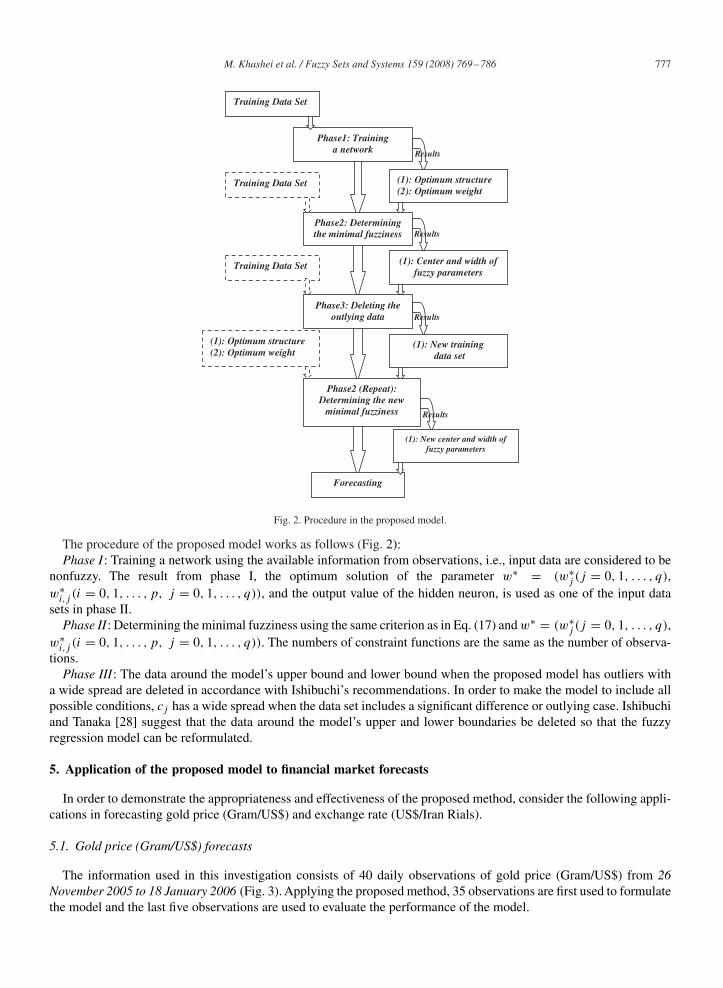
Fig. 2. Procedure in the proposed model.

The procedure of the proposed model works as follows (Fig. 2):Phase I: Training a network using the available information from observations, i.e., input data are considered to be

nonfuzzy. The result from phase I, the optimum solution of the parameter w∗ = (w∗j (j = 0, 1, . . . , q),

w∗i,j (i = 0, 1, . . . , p, j = 0, 1, . . . , q)), and the output value of the hidden neuron, is used as one of the input data

sets in phase II.Phase II: Determining the minimal fuzziness using the same criterion as in Eq. (17) and w∗ = (w∗

j (j = 0, 1, . . . , q),w∗

i,j (i = 0, 1, . . . , p, j = 0, 1, . . . , q)). The numbers of constraint functions are the same as the number of observa-tions.

Phase III: The data around the model’s upper bound and lower bound when the proposed model has outliers witha wide spread are deleted in accordance with Ishibuchi’s recommendations. In order to make the model to include allpossible conditions, cj has a wide spread when the data set includes a significant difference or outlying case. Ishibuchiand Tanaka [28] suggest that the data around the model’s upper and lower boundaries be deleted so that the fuzzyregression model can be reformulated.

5. Application of the proposed model to financial market forecasts

In order to demonstrate the appropriateness and effectiveness of the proposed method, consider the following appli-cations in forecasting gold price (Gram/US$) and exchange rate (US$/Iran Rials).

5.1. Gold price (Gram/US$) forecasts

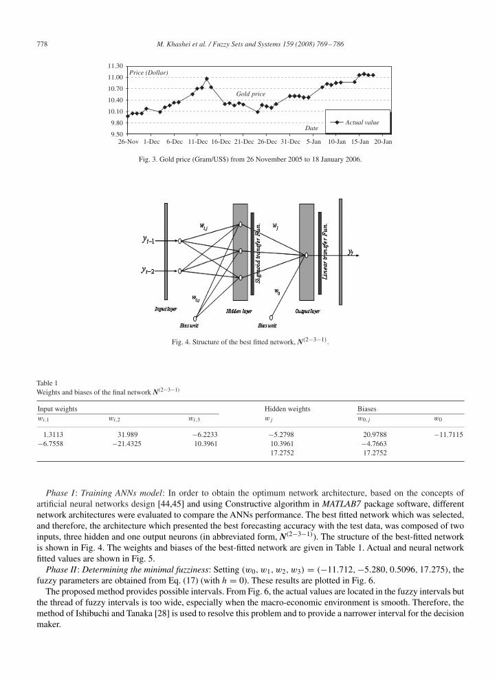
The information used in this investigation consists of 40 daily observations of gold price (Gram/US$) from 26November 2005 to 18 January 2006 (Fig. 3). Applying the proposed method, 35 observations are first used to formulatethe model and the last five observations are used to evaluate the performance of the model.


9.50

9.80

10.10

10.40

10.70

11.00

11.30

26-Nov 1-Dec 6-Dec 11-Dec 16-Dec 21-Dec 26-Dec 31-Dec 5-Jan 10-Jan 15-Jan 20-Jan

Price (Dollar)

Date

Gold price

Actual value

Fig. 3. Gold price (Gram/US$) from 26 November 2005 to 18 January 2006.

Fig. 4. Structure of the best fitted network, N(2−3−1).

Table 1Weights and biases of the final network N(2−3−1)

Input weights Hidden weights Biaseswi,1 wi,2 wi,3 wj w0,j w0

1.3113 31.989 −6.2233 −5.2798 20.9788 −11.7115−6.7558 −21.4325 10.3961 10.3961 −4.7663

17.2752 17.2752

Phase I: Training ANNs model: In order to obtain the optimum network architecture, based on the concepts ofartificial neural networks design [44,45] and using Constructive algorithm in MATLAB7 package software, differentnetwork architectures were evaluated to compare the ANNs performance. The best fitted network which was selected,and therefore, the architecture which presented the best forecasting accuracy with the test data, was composed of twoinputs, three hidden and one output neurons (in abbreviated form, N(2−3−1)). The structure of the best-fitted networkis shown in Fig. 4. The weights and biases of the best-fitted network are given in Table 1. Actual and neural networkfitted values are shown in Fig. 5.

Phase II: Determining the minimal fuzziness: Setting (w0, w1, w2, w3) = (−11.712, −5.280, 0.5096, 17.275), thefuzzy parameters are obtained from Eq. (17) (with h = 0). These results are plotted in Fig. 6.

The proposed method provides possible intervals. From Fig. 6, the actual values are located in the fuzzy intervals butthe thread of fuzzy intervals is too wide, especially when the macro-economic environment is smooth. Therefore, themethod of Ishibuchi and Tanaka [28] is used to resolve this problem and to provide a narrower interval for the decisionmaker.


9.50

9.80

10.10

10.40

10.70

11.00

11.30

28-Nov 3-Dec 8-Dec 13-Dec 18-Dec 23-Dec 28-Dec 2-Jan 7-Jan 12-Jan 17-Jan

Price (Dollar)

Date

Actual value

Fitted value

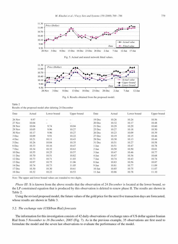
Fig. 5. Actual and neural network fitted values.

9.50

9.80

10.10

10.40

10.70

11.00

11.30

28-Nov 3-Dec 8-Dec 13-Dec 18-Dec 23-Dec 28-Dec 2-Jan 7-Jan 12-Jan

Actual valueUpper boundLower bound

Price (Dollar)

Date

Fig. 6. Results obtained from the proposed model.

Table 2Results of the proposed model after deleting 24 December

Date Actual Lower bound Upper bound Date Actual Lower bound Upper bound

26 Nov 9.97 – – 19 Dec 10.26 10.24 10.5627 Nov 10.04 – – 20 Dec 10.32 10.17 10.4828 Nov 10.04 9.74 10.04 21 Dec 10.29 10.29 10.6029 Nov 10.05 9.96 10.27 25 Dec 10.27 10.18 10.5030 Nov 10.17 9.96 10.27 26 Dec 10.23 10.09 10.393 Dec 10.09 9.91 10.22 27 Dec 10.19 10.15 10.464 Dec 10.21 10.11 10.43 28 Dec 10.30 10.13 10.445 Dec 10.26 10.04 10.35 31 Dec 10.51 10.27 10.586 Dec 10.33 10.16 10.47 1 Jan 10.51 10.47 10.787 Dec 10.34 10.32 10.63 2 Jan 10.50 10.50 10.8110 Dec 10.55 10.25 10.57 3 Jan 10.47 10.46 10.7711 Dec 10.70 10.51 10.82 4 Jan 10.47 10.36 10.6812 Dec 10.73 10.71 11.03 7 Jan 10.74 10.43 10.7413 Dec 10.97 10.75 11.06 8 Jan 10.83 10.56 10.8714 Dec 10.74 10.73 11.05 9 Jan 10.81 10.77 11.0917 Dec 10.30 10.30 10.61 10 Jan 10.85 10.75 11.0718 Dec 10.32 10.22 10.53 11 Jan 10.86 10.78 11.10

Note: The upper and lower bound values are rounded to two digits.

Phase III: It is known from the above results that the observation of 24 December is located at the lower bound, sothe LP constrained equation that is produced by this observation is deleted to renew phase II. The results are shown inTable 2.

Using the revised proposed model, the future values of the gold price for the next five transaction days are forecasted,whose results are shown in Table 3.

5.2. The exchange rate (US$/Iran Rial) forecasts

The information for this investigation consists of 42 daily observations of exchange rates of US dollar against IranianRial from 5 November to 16 December, 2005 (Fig. 7). As in the previous example, 35 observations are first used toformulate the model and the seven last observations to evaluate the performance of the model.


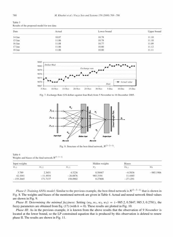
Table 3Results of the proposed model for test data

Date Actual Lower bound Upper bound

14 Jan 10.87 10.78 11.1015 Jan 11.06 10.78 11.1016 Jan 11.08 10.77 11.0917 Jan 11.06 10.80 11.1218 Jan 11.06 10.80 11.11

9067

9070

9073

9076

9079

9082

9085

5-Nov 10-Nov 15-Nov 20-Nov 25-Nov 30-Nov 5-Dec 10-Dec 15-Dec

Actual valueDate

Exchange rate

Dollar/ Rial

Fig. 7. Exchange Rate (US dollars against Iran Rial) from 5 November to 16 December 2005.

Fig. 8. Structure of the best-fitted network, N(3−3−1).

Table 4Weights and biases of the final network N(3−3−1)

Input weights Hidden weights Biaseswi,1 wi,2 wi,3 wj w0,j w0

3.789 2.3651 4.5226 0.58467 −6.5836 −985.190642.1041 −11.4934 −26.0876 985.3194 11.4485

−155.2665 171.7137 158.0902 0.27808 −27.1291

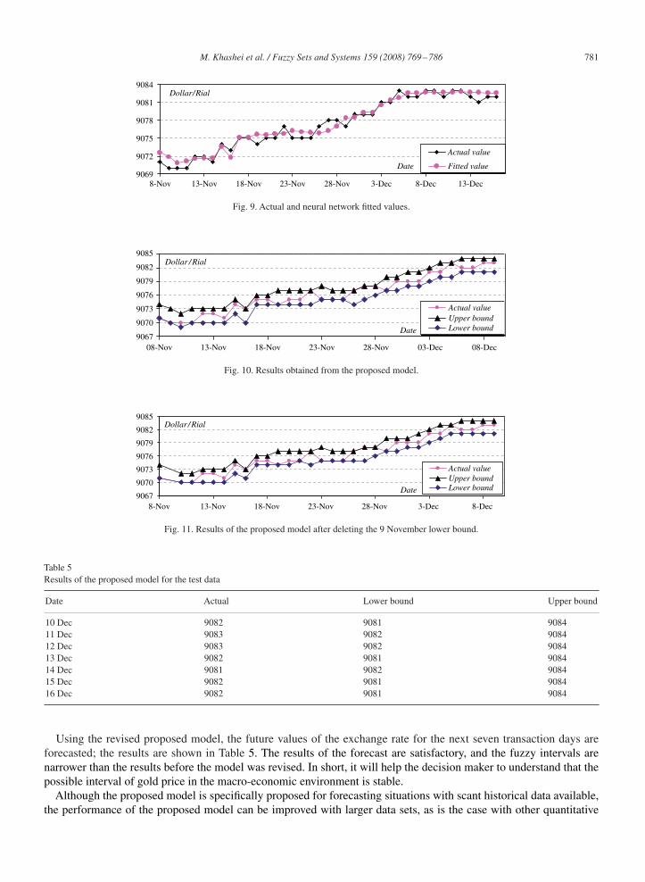
Phase I: Training ANNs model: Similar to the previous example, the best-fitted network is N(3−3−1) that is shown inFig. 8. The weights and biases of the mentioned network are given in Table 4. Actual and neural network fitted valuesare shown in Fig. 9.

Phase II: Determining the minimal fuzziness: Setting (w0, w1, w2, w3) = (−985.2, 0.5847, 985.3, 0.2781), thefuzzy parameters are obtained from Eq. (17) (with h = 0). These results are plotted in Fig. 10.

Phase III: As in the previous example, it is known from the above results that the observation of 9 November islocated at the lower bound, so the LP constrained equation that is produced by this observation is deleted to renewphase II. The results are shown in Fig. 11.


9069

9072

9075

9078

9081

9084

8-Nov 13-Nov 18-Nov 23-Nov 28-Nov 3-Dec 8-Dec 13-Dec

Actual value

Fitted valueDate

Dollar/Rial

Fig. 9. Actual and neural network fitted values.

9067

9070

9073

9076

9079

9082

9085

08-Nov 13-Nov 18-Nov 23-Nov 28-Nov 03-Dec 08-Dec


Dollar /Rial

Date

Fig. 10. Results obtained from the proposed model.

8-Nov9067

9070

9073

9076

9079

9082

9085

13-Nov 18-Nov 23-Nov 28-Nov 3-Dec 8-Dec


Dollar /Rial

Date

Fig. 11. Results of the proposed model after deleting the 9 November lower bound.

Table 5Results of the proposed model for the test data

Date Actual Lower bound Upper bound

10 Dec 9082 9081 908411 Dec 9083 9082 908412 Dec 9083 9082 908413 Dec 9082 9081 908414 Dec 9081 9082 908415 Dec 9082 9081 908416 Dec 9082 9081 9084

Using the revised proposed model, the future values of the exchange rate for the next seven transaction days areforecasted; the results are shown in Table 5. The results of the forecast are satisfactory, and the fuzzy intervals arenarrower than the results before the model was revised. In short, it will help the decision maker to understand that thepossible interval of gold price in the macro-economic environment is stable.

Although the proposed model is specifically proposed for forecasting situations with scant historical data available,the performance of the proposed model can be improved with larger data sets, as is the case with other quantitative


Table 6Comparison of forecasted interval widths of the proposed model with different sample sizes

Sample Size

Series100 200 300 350

Gold price 2.3 2.1 1.9 1.9

Exchange rate 0.29 0.27 0.23 0.21

Table 7Comparison of forecasted interval widths by the proposed model compared to other forecasting models

Model Case Forecasted interval width Related performanceANNs Fuzzy ARIMA Proposed model

ANNs (95% confidence interval) Gold price 1.23 0 – –Fuzzy ARIMA 0.57 53.6% 0 –Proposed model 0.32 74.0% 43.9% 0ANNs (95% confidence interval) Exchange rate 16.2 0 – –Fuzzy ARIMA 4.2 74.1% 0 –Proposed model 2.5 84.6% 40.5% 0

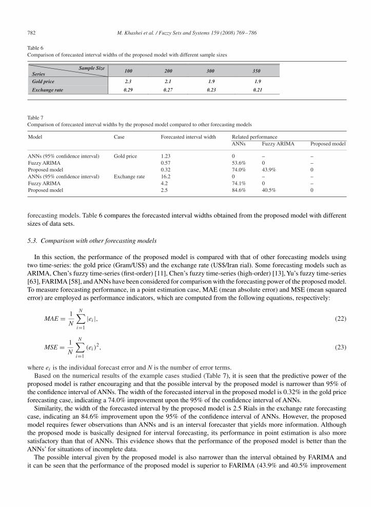
forecasting models. Table 6 compares the forecasted interval widths obtained from the proposed model with differentsizes of data sets.

5.3. Comparison with other forecasting models

In this section, the performance of the proposed model is compared with that of other forecasting models usingtwo time-series: the gold price (Gram/US$) and the exchange rate (US$/Iran rial). Some forecasting models such asARIMA, Chen’s fuzzy time-series (first-order) [11], Chen’s fuzzy time-series (high-order) [13], Yu’s fuzzy time-series[63], FARIMA [58], andANNs have been considered for comparison with the forecasting power of the proposed model.To measure forecasting performance, in a point estimation case, MAE (mean absolute error) and MSE (mean squarederror) are employed as performance indicators, which are computed from the following equations, respectively:

MAE = 1

N

N∑i=1

|ei |, (22)

MSE = 1

N

N∑i=1

(ei)2, (23)

where ei is the individual forecast error and N is the number of error terms.Based on the numerical results of the example cases studied (Table 7), it is seen that the predictive power of the

proposed model is rather encouraging and that the possible interval by the proposed model is narrower than 95% ofthe confidence interval of ANNs. The width of the forecasted interval in the proposed model is 0.32% in the gold priceforecasting case, indicating a 74.0% improvement upon the 95% of the confidence interval of ANNs.

Similarity, the width of the forecasted interval by the proposed model is 2.5 Rials in the exchange rate forecastingcase, indicating an 84.6% improvement upon the 95% of the confidence interval of ANNs. However, the proposedmodel requires fewer observations than ANNs and is an interval forecaster that yields more information. Althoughthe proposed mode is basically designed for interval forecasting, its performance in point estimation is also moresatisfactory than that of ANNs. This evidence shows that the performance of the proposed model is better than theANNs’ for situations of incomplete data.

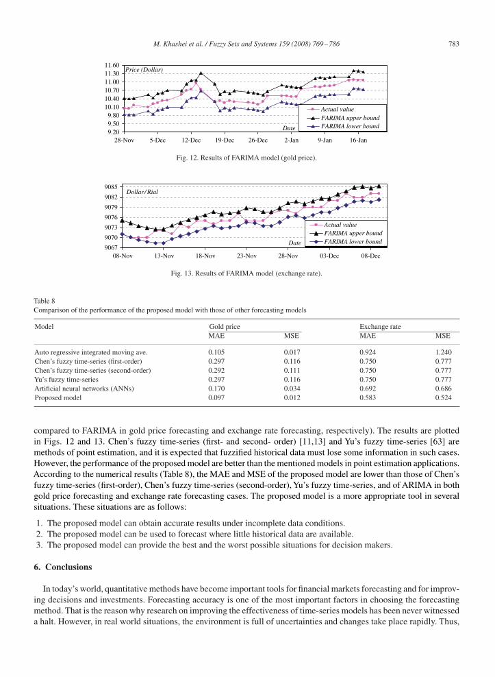
The possible interval given by the proposed model is also narrower than the interval obtained by FARIMA andit can be seen that the performance of the proposed model is superior to FARIMA (43.9% and 40.5% improvement


9.209.509.80

10.1010.4010.7011.0011.3011.60

28-Nov 5-Dec 12-Dec 19-Dec 26-Dec 2-Jan 9-Jan 16-Jan

Actual valueFARIMA upper boundFARIMA lower bound

Price (Dollar)

Date

Fig. 12. Results of FARIMA model (gold price).

9067

9070

9073

9076

9079

9082

9085

08-Nov 13-Nov 18-Nov 23-Nov 28-Nov 03-Dec 08-Dec

Actual valueFARIMA upper boundFARIMA lower bound

Dollar/ Rial

Date

Fig. 13. Results of FARIMA model (exchange rate).

Table 8Comparison of the performance of the proposed model with those of other forecasting models

Model Gold price Exchange rateMAE MSE MAE MSE

Auto regressive integrated moving ave. 0.105 0.017 0.924 1.240Chen’s fuzzy time-series (first-order) 0.297 0.116 0.750 0.777Chen’s fuzzy time-series (second-order) 0.292 0.111 0.750 0.777Yu’s fuzzy time-series 0.297 0.116 0.750 0.777Artificial neural networks (ANNs) 0.170 0.034 0.692 0.686Proposed model 0.097 0.012 0.583 0.524

compared to FARIMA in gold price forecasting and exchange rate forecasting, respectively). The results are plottedin Figs. 12 and 13. Chen’s fuzzy time-series (first- and second- order) [11,13] and Yu’s fuzzy time-series [63] aremethods of point estimation, and it is expected that fuzzified historical data must lose some information in such cases.However, the performance of the proposed model are better than the mentioned models in point estimation applications.According to the numerical results (Table 8), the MAE and MSE of the proposed model are lower than those of Chen’sfuzzy time-series (first-order), Chen’s fuzzy time-series (second-order), Yu’s fuzzy time-series, and of ARIMA in bothgold price forecasting and exchange rate forecasting cases. The proposed model is a more appropriate tool in severalsituations. These situations are as follows:

1. The proposed model can obtain accurate results under incomplete data conditions.2. The proposed model can be used to forecast where little historical data are available.3. The proposed model can provide the best and the worst possible situations for decision makers.

6. Conclusions

In today’s world, quantitative methods have become important tools for financial markets forecasting and for improv-ing decisions and investments. Forecasting accuracy is one of the most important factors in choosing the forecastingmethod. That is the reason why research on improving the effectiveness of time-series models has been never witnesseda halt. However, in real world situations, the environment is full of uncertainties and changes take place rapidly. Thus,


future situations must be usually forecasted using little data from a short span of time. In this paper, based on thebasic concepts of the artificial neural networks (ANNs) and fuzzy regression, a new method is proposed and applied toforecasting in financial markets in an attempt to show the appropriateness and effectiveness of our proposed method.In this method, the limitation of a large amount of historical data is lifted through investing on the advantages ofthe fuzzy regression models. The proposed model, therefore, requires fewer observations than does ANNs to obtainaccurate results. The proposed model also obtains narrower possible intervals than other interval-forecasting models dounder incomplete data conditions, by exploiting the advantage of the artificial neural networks (ANNs) to preprocessthe raw data. The empirical results obtained from forecasting in financial markets indicate that the proposed modelis a suitable model for use in incomplete data situations. The performance of the proposed model is better than thefuzzy and nonfuzzy models surveyed here. It is additionally a suitable model for both point and interval forecasts withincomplete data. From the empirical results, it can be seen that the proposed method cannot only make good forecastsbut also provide the decision makers with the best and worst possible situations. Therefore, it outperforms its rivals.

Acknowledgments

The authors wish to express their gratitude to the referees and Gh. A. Raissi, Assistant Professor of IndustrialEngineering, Isfahan University of Technology, without whose assistance this work could never have become possible.

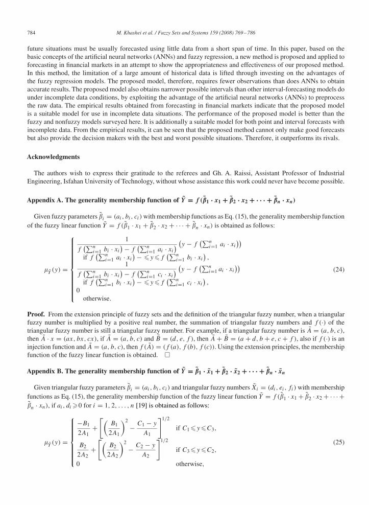
Appendix A. The generality membership function of Y = f (�1 · x1 + �2 · x2 + · · · + �n · xn)

Given fuzzy parameters �i = (ai, bi, ci) with membership functions as Eq. (15), the generality membership functionof the fuzzy linear function Y = f (�1 · x1 + �2 · x2 + · · · + �n · xn) is obtained as follows:

�Y(y) =

⎧⎪⎪⎪⎪⎪⎪⎪⎪⎪⎪⎨⎪⎪⎪⎪⎪⎪⎪⎪⎪⎪⎩

1

f(∑n

i=1 bi · xi

)− f(∑n

i=1 ai · xi

) (y − f(∑n

i=1 ai · xi

))if f

(∑ni=1 ai · xi

)− �y�f(∑n

i=1 bi · xi

),

1

f(∑n

i=1 bi · xi

)− f(∑n

i=1 ci · xi

) (y − f(∑n

i=1 ai · xi

))if f

(∑ni=1 bi · xi

)− �y�f(∑n

i=1 ci · xi

),

0otherwise.

(24)

Proof. From the extension principle of fuzzy sets and the definition of the triangular fuzzy number, when a triangularfuzzy number is multiplied by a positive real number, the summation of triangular fuzzy numbers and f (·) of thetriangular fuzzy number is still a triangular fuzzy number. For example, if a triangular fuzzy number is A = (a, b, c),then A · x = (ax, bx, cx), if A = (a, b, c) and B = (d, e, f ), then A + B = (a + d, b + e, c + f ), also if f (·) is aninjection function and A = (a, b, c), then f (A) = (f (a), f (b), f (c)). Using the extension principles, the membershipfunction of the fuzzy linear function is obtained. �

Appendix B. The generality membership function of Y = �1 · x1 + �2 · x2 + · · · + �n · xn

Given triangular fuzzy parameters �i = (ai, bi, ci) and triangular fuzzy numbers Xi = (di, ei, fi) with membershipfunctions as Eq. (15), the generality membership function of the fuzzy linear function Y = f (�1 · x1 + �2 · x2 + · · · +�n · xn), if ai, di �0 for i = 1, 2, . . . , n [19] is obtained as follows:

�Y(y) =

⎧⎪⎪⎪⎪⎪⎪⎨⎪⎪⎪⎪⎪⎪⎩

−B1

2A1+[(

B1

2A1

)2

− C1 − y

A1

]1/2

if C1 �y�C3,

B2

2A2+[(

B2

2A2

)2

− C2 − y

A2

]1/2

if C3 �y�C2,

0 otherwise,

(25)


where

A1 =n∑

i=1

(bi − ai)(ei − di), A2 =n∑

i=1

(ci − bi)(fi − ei),

B1 =n∑

i=1

(ai(ei − di) + di(bi − ai)), B2 =n∑

i=1

(ci(fi − ei) + fi(ci − bi)),

C1 =n∑

i=1

(aidi), C2 =n∑

i=1

(cifi), C3 =n∑

i=1

(biei).

Proof. From the relationship functions of the fuzzy number �i and Xi , the �-cut interval sets for the two fuzzynumbers are ��

i = [ai + �(bi − ai), ci + �(bi − ci)] and X�i = [di + �(ei − di), fi + �(ei − fi)], respectively. By

the extension principle of fuzzy sets, the multiplication of two �-cut interval sets causes a �-cut interval set as Z�i =

��i · X�

i = [ai + �(bi − ai)] × [di + �(ei − di)], [ci + �(bi − ci)] × [fi + �(ei − fi)]. The membership function ofthe fuzzy number Z�

i is facile [33]. �

References

[1] J. Arifovic, R. Gencay, Using genetic algorithms to select architecture of a feed-forward artificial neural network, Phys. A 289 (2001) 574–594.[2] G. Armano, M. Marchesi, A. Murru, A hybrid genetic-neural architecture for stock indexes forecasting, Inform. Sci. 170 (2005) 3–33.[3] S.D. Balkin, J.K. Ord, Automatic neural network modeling for univariate time series, Internat. J. Forecasting 16 (2000) 509–515.[4] J.M. Bates, W.J. Granger, The combination of forecasts, Comput. Oper. Res. 20 (1969) 451–468.[5] P.G. Benardos, G.C.Vosniakos, Prediction of surface roughness in CNC face milling using neural networks and Taguchi’s design of experiments,

Robotics and Computer Integrated Manufacturing 18 (2002) 343–354.[6] P.G. Benardos, G.C. Vosniakos, Optimizing feed-forward artificial neural network architecture, Eng. Appl. of Artificial Intelligence 20 (2007)

365–382.[7] G.P. Box, G.M. Jenkins, Time Series Analysis: Forecasting and Control, Holden-Day, San Francisco, CA, 1976.[8] P.A. Castillo, J.J. Merelo, A. Prieto, V. Rivas, G. Romero, GProp: global optimization of multilayer perceptrons using GA, Neurocomputing

35 (2000) 149–163.[9] P.T. Chang, Fuzzy seasonality forecasting, Fuzzy Sets and Systems 90 (1997) 1–10.

[10] A. Chen, M.T. Leung, D. Hazem, Application of neural networks to an emerging financial market: forecasting and trading the Taiwan StockIndex, Comput. Oper. Res. 30 (2003) 901–923.

[11] S.M. Chen, Forecasting enrollments based on fuzzy time series, Fuzzy Sets and Systems 81 (3) (1996) 311–319.[12] S.M. Chen, Forecasting enrollments based on high-order fuzzy time series, Cybernet Systems 33 (2002) 1–16.[13] S.M. Chen, N.Y. Chung, Forecasting enrollments using high-order fuzzy time series and genetic algorithms, Internat. J. Intell. Syst. 21 (2006)

485–501.[14] S.M. Chen, C.C. Hsu, A new method to forecast enrollments using fuzzy time series, Appl. Sci. Eng. 2 (2004) 234–244.[15] S.M. Chen, J.R. Hwang, Temperature prediction using fuzzy time series, IEEE Trans. Systems Man Cybernet B 30 (2) (2000) 263–275.[16] R. Clemen, Combining forecasts: a review and annotated bibliography with discussion, Internat. J. Forecasting 5 (1989) 559–608.[17] H. Demuth, B. Beale, Neural Network Toolbox User Guide, The Math Works Inc., Natick, 2004.[18] D. Dubois, H. Prade, Theory and Applications, Fuzzy Sets and Systems, Academic Press, New York, 1980.[19] D.H. Hong, H.C. Yi, A note on fuzzy regression model with fuzzy input and output data for manpower forecasting, Fuzzy Sets and Systems

138 (2003) 301–305.[20] H. Hosseini, D. Luo, K.J. Reynolds, The comparison of different feed forward neural network architectures for ECG signal diagnosis, Medical

Eng. Phys. 28 (2006) 372–378.[21] Y.Y. Hsu, S.M. Tse, B. Wu, A new approach of bivariate fuzzy time series analysis to the forecasting of a stock index, Internat. J. Uncertainty,

Fuzziness and Knowledge Based Systems 11 (6) (2003) 671–690.[22] K. Huarng, Effective lengths of intervals to improve forecasting in fuzzy time series, Fuzzy Sets and Systems 123 (2001) 387–394.[23] K. Huarng, Heuristic models of fuzzy time series for forecasting, Fuzzy Sets and Systems 123 (2001) 137–154.[24] K. Huarng, H.-K. Yu, An N-th order heuristic fuzzy time series model for TAIEX forecasting, Internat. J. Fuzzy Systems 5 (4) (2003).[25] K. Huarng, H.K. Yu, A Type 2 fuzzy time series model for stock index forecasting, Phys. A 353 (2005) 445–462.[26] K. Huarng, T.H.K. Yu, The application of neural networks to forecast fuzzy time series, Phys. A 336 (2006) 481–491.[27] J.R. Hwang, S.M. Chen, C.H. Lee, Handling forecasting problems using fuzzy time series, Fuzzy Sets and Systems 100 (1998) 217–228.[28] H. Ishibuchi, H. Tanaka, Interval regression analysis based on mixed 0–1 integer programming problem, J. Japan Soc. Ind. Eng. 40 (5) (1988)

312–319.[29] M.M. Islam, K. Murase, A new algorithm to design compact two hidden-layer artificial neural networks, Neural Networks 14 (2001)

1265–1278.


[30] X. Jiang, A.H.K.S. Wah, Constructing and training feed-forward neural networks for pattern classification, Pattern Recognition 36 (2003)853–867.

[31] S. Kang, An Investigation of the Use of Feed forward Neural Networks for Forecasting, Ph.D. Thesis, Kent State University, 1991.[32] M. Khashei, Forecasting the Isfahan Steel Company production price in Tehran Metals Exchange using artificial neural networks (ANNs),

Master of Science Thesis, Isfahan University of Technology, 2005.[33] H.T. Lee, S.H. Chen, Fuzzy regression model with fuzzy input and output data for manpower forecasting, Fuzzy Sets and Systems 119 (2001)

205–213.[34] J. Lee, S. Kang, GA based meta-modeling of BPN architecture for constrained approximate optimization, Internat. J. Solids and Structures 44

(2007) 5980–5993.[35] C.H. Leon, A. Liu, W.S. Chen, Pattern discovery of fuzzy time series for financial prediction, IEEE Trans. Knowl. Data Eng. 18 (2006)

613–625.[36] J. Leski, E. Czogala,A new artificial network based fuzzy interference system with moving consequents in if–then rules and selected applications,

Fuzzy Sets and Systems 108 (1999) 289–297.[37] J.T. Luxhoj, J.O. Riis, B. Stensballe, A hybrid econometric-neural network modeling approach for sales forecasting, Internat. J. Prod. Econom.

43 (1996) 175–192.[38] L. Ma, K. Khorasani, A new strategy for adaptively constructing multilayer feed-forward neural networks, Neurocomputing 51 (2003)

361–385.[39] H.R. Maier, G.C. Dandy, The effect of internal parameters and geometry on the performance of back-propagation neural networks: an empirical

study, Environmental Modeling & Software 13 (1998) 193–209.[40] D. Marin, A. Varo, J.E. Guerrero, Non-linear regression methods in NIRS quantitative analysis, Talanta 72 (2007) 28–42.[41] G.A. Miller, The magical number seven, plus or minus two: some limits on our capacity of processing information, Psychol. Rev. 63 (1956)

81–97.[42] K. Nam, T. Schaefer, Forecasting international airline passenger traffic using neural networks, Logistics and Transportation 31 (3) (1995)

239–251.[43] G.E. Nasr, E.A. Badr, C. Joun, Back propagation neural networks for modeling gasoline consumption, Energy Conversion and Management

44 (2003) 893–905.[44] A. Palmer, J. Jose, A. Sese, Designing an artificial neural network for forecasting tourism time series, Tourism Management 26 (2006)

781–790.[45] M.Y. Rafiq, G. Bugmann, D.J. Easterbrook, Neural network design for engineering applications, Comput. Structures 79 (2001) 1541–1552.[46] M.J. Reid, Combining three estimates of gross domestic product, Economica 35 (1968) 431–444.[47] J.P. Ross, Taguchi Techniques for Quality Engineering, McGraw-Hill, New York, 1996.[48] K. Smith, N.D. Jatinder, Neural networks in business: techniques and applications for the operations researcher, Comput. Oper. Res. 27 (2000)

1045–1076.[49] Q. Song, Seasonal forecasting in fuzzy time series, Fuzzy Sets and Systems 107 (1999) 235–236.[50] Q. Song, B.S. Chissom, Forecasting enrollments with fuzzy time series—(part I), Fuzzy Sets and Systems 54 (1) (1993) 1–9.[51] Q. Song, B.S. Chissom, Fuzzy time series and its models, Fuzzy Sets and Systems 54 (1993) 269–277.[52] Q. Song, B.S. Chissom, Forecasting enrollments with fuzzy time series—(part II), Fuzzy Sets and Systems 62 (1) (1994) 1–8.[53] J. Sullivan, W.H. Woodall, A comparison of fuzzy forecasting and Markov modeling, Fuzzy Sets and Systems 64 (1994) 279–293.[54] H. Tanaka, Fuzzy data analysis by possibility linear models, Fuzzy Sets and Systems 24 (3) (1987) 363–375.[55] H. Tanaka, H. Ishibuchi, Possibility regression analysis based on linear programming, in: J. Kacprzyk, M. Fedrizzi (Eds.), Fuzzy Regression

Analysis, Omnitech Press, Warsaw and Physica-Verlag, Heidelberg, 1992, pp. 47–60.[56] H. Tanaka, S. Uejima, K. Asai, Linear regression analysis with fuzzy model, IEEE Trans. Systems Man Cybernet. 12 (6) (1982) 903–907.[57] S. Thawornwong, D. Enke, The adaptive selection of financial and economic variables for use with artificial neural networks, Neurocomputing

31 (2000) 1–13.[58] F. Tseng, G. Tzeng, H.C. Yu, B.J.C. Yuana, Fuzzy ARIMA model for forecasting the foreign exchange market, Fuzzy Sets and Systems 118

(2001) 9–19.[59] M. Versaci, F.C. Morabito, Fuzzy time series approach for disruption prediction in Tokamak reactors, IEEE Trans. Magnetics 39 (3) (2003)

1503–1506.[60] Y.F. Wang, Predicting stock price using fuzzy grey prediction system, Experts Systems with Applications 22 (2002) 33–39.[61] J. Watada, Fuzzy time series analysis and forecasting of sales volume, in: J. Kacprzyk, M. Fedrizzi (Eds.), Fuzzy Regression Analysis, Omnitech

Press, Warsaw and Physica-Verlag, Heidelberg, 1992, pp. 211–227.[62] B.K. Wong, S. Vincent, L. Jolie, A bibliography of neural network business applications research: 1994–1998, Comput. Oper. Res. 27 (2000)

1023–1044.[63] H.K. Yu, Weighted fuzzy time-series models for TAIEX forecasting, Phys. A 349 (2004) 609–624.[64] H.K. Yu, A refined fuzzy time-series model for forecasting, Phys. A 346 (3–4) (2005) 657–681.[65] L.A. Zadeh, The concept of a linguistic variable and its application to approximate reasoning I, Inform. Sci. 8 (1975) 199–249.[66] L.A. Zadeh, The concept of a linguistic variable and its application to approximate reasoning II, Inform. Sci. 8 (1975) 301–357.[67] L.A. Zadeh, The concept of a linguistic variable and its application to approximate reasoning III, Inform. Sci. 9 (1976) 43–80.[68] G.P. Zhang, B.E. Hu, Forecasting with artificial neural networks: the state of the art, Neurocomputing 56 (2004) 205–232.[69] P. Zhang, G. Min Qi, Neural network forecasting for seasonal and trend time series, European J. Oper. Res. 160 (2005) 501–514.

A new hybrid artificial neural networks and fuzzy regression model for time series forecasting

Documents