A new feature weighted fuzzy clustering algorithm

IADIS EUROPEAN CONFERENCE ON DATA MINING 2009

part of the

IADIS MULTI CONFERENCE ON COMPUTER SCIENCE AND

INFORMATION SYSTEMS 2009

ii

iii

PROCEEDINGS OF THE IADIS EUROPEAN CONFERENCE ON

DATA MINIG 2009

part of the

IADIS MULTI CONFERENCE ON COMPUTER SCIENCE AND

INFORMATION SYSTEMS 2009

Algarve, Portugal

JUNE 18 - 20, 2009

Organised by IADIS

International Association for Development of the Information Society

iv

Copyright 2009

IADIS Press

All rights reserved

This work is subject to copyright. All rights are reserved, whether the whole or part of the material is concerned, specifically the rights of translation, reprinting, re-use of illustrations, recitation,

broadcasting, reproduction on microfilms or in any other way, and storage in data banks. Permission for use must always be obtained from IADIS Press. Please contact [email protected]

Data Mining Volume Editor: Ajith P. Abraham

Computer Science and Information Systems Series Editors:

Piet Kommers, Pedro Isaías and Nian-Shing Chen

Associate Editors: Luís Rodrigues and Patrícia Barbosa

ISBN: 978-972-8924-88-1

SUPPORTED BY

v

TABLE OF CONTENTS

FOREWORD ix

PROGRAM COMMITTEE xi

KEYNOTE LECTURES xv

CONFERENCE TUTORIAL xviii

KEYNOTE PAPER xix

FULL PAPERS

AN EXPERIMENTAL STUDY OF THE DISTRIBUTED CLUSTERING FOR AIR POLLUTION PATTERN RECOGNITION IN SENSOR NETWORKS Yajie Ma, Yike Guo and Moustafa Ghanem

3

A NEW FEATURE WEIGHTED FUZZY C-MEANS CLUSTERING ALGORITHM Huaiguo Fu and Ahmed M. Elmisery

11

A NOVEL THREE STAGED CLUSTERING ALGORITHM Jamil Al-Shaqsi and Wenjia Wang

19

BEHAVIOURAL FINANCE AS A MULTI-INSTANCE LEARNING PROBLEM Piotr Juszczak

27

BATCH QUERY SELECTION IN ACTIVE LEARNING Piotr Juszczak

35

CONTINUOUS-TIME HIDDEN MARKOV MODELS FOR THE COPY NUMBER ANALYSIS OF GENOTYPING ARRAYS Matthew Kowgier and Rafal Kustra

43

OUT-OF-CORE DATA HANDLING WITH PERIODIC PARTIAL RESULT MERGING Sándor Juhász and Renáta Iváncsy

50

A FUZZY WEB ANALYTICS MODEL FOR WEB MINING Darius Zumstein and Michael Kaufmann

59

DATE-BASED DYNAMIC CACHING MECHANISM Christos Bouras, Vassilis Poulopoulos and Panagiotis Silintziris

67

vi

GENETIC ALGORITHM TO DETERMINE RELEVANT FEATURES FOR INTRUSION DETECTION Namita Aggarwal, R K Agrawal and H M Jain

75

ACCURATELY RANKING OUTLIERS IN DATA WITH MIXTURE OF VARIANCES AND NOISE Minh Quoc Nguyen, Edward Omiecinski and Leo Mark

83

TIME SERIES DATA PUBLISHING AND MINING SYSTEM Ye Zhu, Yongjian Fu and Huirong Fu

95

UNIFYING THE SYNTAX OF ASSOCIATION RULES Michal Burda

103

AN APPROACH TO VARIABLE SELECTION IN EFFICIENCY ANALYSIS Veska Noncheva, Armando Mendes and Emiliana Silva

111

SHORT PAPERS

MIDPDC: A NEW FRAMEWORK TO SUPPORT DIGITAL MAMMOGRAM DIAGNOSIS Jagatheesan Senthilkumar, A. Ezhilarasi and D. Manjula

121

A TWO-STAGE APPROACH FOR RELEVANT GENE SELECTION FOR CANCER CLASSIFICATION Rajni Bala and R. K. Agrawal

127

TARGEN: A MARKET BASKET DATASET GENERATOR FOR TEMPORAL ASSOCIATION RULE MINING Tim Schlüter and Stefan Conrad

133

USING TEXT CATEGORISATION FOR DETECTING USER ACTIVITY Marko Kääramees and Raido Paaslepp

139

APPROACHES FOR EFFICIENT HANDLING OF LARGE DATASETS Renáta Iváncsy and Sándor Juhász

143

GROUPING OF ACTORS ON AN ENTERPRISE SOCIAL NETWORK USING OPTIMIZED UNION-FIND ALGORITHM Aasma Zahid, Umar Muneer, Shoab A. Khan

148

APPLYING ASD-DM METHODOLOGY ON BUSINESS INTELLIGENCE SOLUTIONS: A CASE STUDY ON BUILDING CUSTOMER CARE DATA MART Mouhib Alnoukari and Zaidoun Alzoabi and Asim El Sheikh

153

COMPARING PREDICTIONS OF MACHINE SPEEDUPS USING MICRO-ARCHITECTURE INDEPENDENT CHARACTERISTICS Claudio Luiz Curotto

158

vii

DDG-CLUSTERING: A NOVEL TECHNIQUE FOR HIGHLY ACCURATE RESULTS Zahraa Said Ammar and Mohamed Medhat Gaber

163

POSTERS

WIEBMAT, A NEW INFORMATION EXTRACTION SYSTEMEN El ouerkhaoui Asmaa, Driss Aboutajdine and Doukkali Aziz

171

CLUSTER OF REUTERS 21578 COLLECTIONS USING GENETIC ALGORITHMS AND NZIPF METHOD José Luis Castillo Sequera, José R. Fernández del Castillo and León González Sotos

174

I-SOAS DATA REPOSITORY FOR ADVANCED PRODUCT DATA MANAGEMENT Zeeshan Ahmed

177

DATA PREPROCESSING DEPENDENCY FOR WEB USAGE MINING BASED ON SEQUENCE RULE ANALYSIS Michal Munk, Jozef Kapusta and Peter Švec

179

GEOGRAPHIC DATA MINING WITH GRR Lubomír Popelínský

182

AUTHOR INDEX

viii

ix

FOREWORD These proceedings contain the papers of the IADIS European Conference on Data Mining 2009, which was organised by the International Association for Development of the Information Society in Algarve, Portugal, 18 – 20 June, 2009. This conference is part of the Multi Conference on Computer Science and Information Systems 2009, 17 - 23 June 2009, which had a total of 1131 submissions. The IADIS European Conference on Data Mining (ECDM’09) is aimed to gather researchers and application developers from a wide range of data mining related areas such as statistics, computational intelligence, pattern recognition, databases and visualization. ECDM’09 is aimed to advance the state of the art in data mining field and its various real world applications. ECDM’09 will provide opportunities for technical collaboration among data mining and machine learning researchers around the globe The conference accepts submissions in the following areas: Core Data Mining Topics - Parallel and distributed data mining algorithms - Data streams mining - Graph mining - Spatial data mining - Text video, multimedia data mining - Web mining - Pre-processing techniques - Visualization - Security and information hiding in data mining Data Mining Applications - Databases, - Bioinformatics, - Biometrics - Image analysis - Financial modeling - Forecasting - Classification - Clustering

x

The IADIS European Conference on Data Mining 2009 received 63 submissions from more than 19 countries. Each submission has been anonymously reviewed by an average of five independent reviewers, to ensure that accepted submissions were of a high standard. Consequently only 14 full papers were published which means an acceptance rate of about 22 %. A few more papers were accepted as short papers, reflection papers and posters. An extended version of the best papers will be published in the IADIS International Journal on Computer Science and Information Systems (ISSN: 1646-3692) and also in other selected journals, including journals from Inderscience. Besides the presentation of full papers, short papers, reflection papers and posters, the conference also included two keynote presentations from internationally distinguished researchers. We would therefore like to express our gratitude to Professor Kurosh Madani, Images, Signals and Intelligence Systems Laboratory (LISSI / EA 3956) PARIS XII University, Senart-Fontainebleau Institute of Technology, France and Dr. Claude C. Chibelushi, Faculty of Computing, Engineering & Technology, Staffordshire University, UK for accepting our invitation as keynote speakers. Also thanks to the tutorial presenter, Professor Kurosh Madani, Images, Signals and Intelligence Systems Laboratory (LISSI / EA 3956) PARIS XII University, Senart-Fontainebleau Institute of Technology, France. As we all know, organising a conference requires the effort of many individuals. We would like to thank all members of the Program Committee, for their hard work in reviewing and selecting the papers that appear in the proceedings. This volume has taken shape as a result of the contributions from a number of individuals. We are grateful to all authors who have submitted their papers to enrich the conference proceedings. We wish to thank all members of the organizing committee, delegates, invitees and guests whose contribution and involvement are crucial for the success of the conference. Last but not the least, we hope that everybody will have a good time in Algarve, and we invite all participants for the next year edition of the IADIS European Conference on Data Mining 2010, that will be held in Freiburg, Germany. Ajith P. Abraham School of Computer Science, Chung-Ang University South Korea European Conference on Data Mining 2009 Program Chair Piet Kommers, University of Twente, The Netherlands Pedro Isaías, Universidade Aberta (Portuguese Open University), Portugal Nian-Shing Chen, National Sun Yat-sen University, Taiwan MCCSIS 2009 General Conference Co-Chairs Algarve, Portugal June 2009

xi

PROGRAM COMMITTEE

EUROPEAN CONFERENCE ON DATA MINING PROGRAM CHAIR

Ajith P. Abraham, School of Computer Science, Chung-Ang University, South Korea

MCCSIS GENERAL CONFERENCE CO-CHAIRS

Piet Kommers, University of Twente, The Netherlands

Pedro Isaías, Universidade Aberta (Portuguese Open University), Portugal

Nian-Shing Chen, National Sun Yat-sen University, Taiwan

EUROPEAN CONFERENCE ON DATA MINING COMMITTEE MEMBERS

Abdel-Badeeh M. Salem, Ain Shams University, Egypt Akihiro Inokuchi, Osaka University, Japan

Alessandra Raffaetà, Università Ca' Foscari di Venezia, Italy Alexandros Nanopoulos, University of Hildesheim, Germany

Alfredo Cuzzocrea, University of Calabria, Italy Anastasios Dimou, Informatics and Telematics Institute, Greece

Andreas König, TU Kaiserslautern, Germany Annalisa Appice, Università degli Studi di Bari, Italy

Arnab Bhattacharya, I.I.T. Kanpur, India Artchil Maysuradze, Moscow University, Russia

Ben Kao, The University of Hong Kong, Hong Kong Carson Leung, University of Manitoba, Canada

Chao Luo, University of Technology, Sydney, Australia Christos Makris, University of Patras, Greece

Claudio Lucchese, Università Ca' Foscari di Venezia, Italy Claudio Silvestri, Università di Ca' Foscari di Venezia, Italy

Dan Wu, University of Windsor, Canada Daniel Kudenko, University of York, UK

Daniel Pop, University of the West Timisoara, Romania Daniela Zaharie, West University of Timisoara, Romania

Daoqiang Zhang, Nanjing University of Aeronautics and Astronautics, China David Cheung, University of Hong Kong, Hong Kong

Dimitrios Katsaros, University of Thessaly, Greece Dino Ienco, Università di Torino, Italy

Edward Hung, Hong Kong Polytechnic University, Hong Kong

xii

Eugenio Cesario, Università della Calabria, Italy Fotis Lazarinis, Technological Educational Institute, Greece

Francesco Folino, University of Calabria, Italy Gabriela Kokai, Friedrich Alexander University, Germany

George Pallis, University of Cyprus, Cyprus Georgios Yannakakis, IT-University of Copenhagen, Denmark

Hamed Nassar, Suez Canal University, Egypt Harish Karnick, IIT Kanpur, India

Hui Xiong, Rutgers University, USA Ingrid Fischer, University of Konstanz, Germany

Ioannis Kopanakis, Technological Educational Institute of Crete, Greece Jason Wang, New Jersey Institute of Technology, USA

Jia -Yu Pan, Google Inc., USA Jialie Shen, Singapore Management University, Singapore

John Kouris, University of Patras, Greece José M. Peña, Technical University of Madrid, Spain

Jun Huan, University of Kansas, USA Junjie Wu, Beijing University of Aeronautics and Astronautics, China

Justin Dauwels, MIT, USA Katia Lida Kermanidis, Ionian University, Greece

Keiichi Horio, Kyushu Institute of Technology, Japan Lefteris Angelis, Aristotle University of Thessaloniki, Greece

Liang Chen, Amazon.com, USA Lyudmila Shulga, Moscow University, Russia

Manolis Maragoudakis, University of Crete, Greece Mario Koeppen, KIT, Japan

Maurizio Atzori, ISTI-CNR, Italy Minlie Huang, Tsinghua University, China Min-Ling Zhang, Hohai University, China Miriam Baglioni, University of Pisa, Italy Qi Li, Western Kentucky University, USA

Raffaele Perego, ISTI-CNR, Italy Ranieri Baraglia, Italian National Research Council (CNR), Italy

Reda Alhajj, University of Calgary, Canada Robert Hilderman, University of Regina, Canada

Roberto Esposito, Università di Torino, Italy Sandeep Pandey, Yahoo! Research,USA Sherry Y. Chen, Brunel University, UK

Stefanos Vrochidis, Informatics and Telematics Institute, Greece Tao Ban, National Institute of Information and Communications Technology, Japan

Tao Li, Florida International University, USA Tao Xiong, eBay Inc., USA

Tatiana Tambouratzis, University of Piraeus, Greece

xiii

Themis Palpanas, University of Trento, Italy Thorsten Meinl, University of Konstanz, Germany

Tianming Hu, Dongguan University of Technology, China Tomonobu Ozaki, Kobe University, Japan Trevor Dix, Monash University, Australia

Tsuyoshi Ide, IBM Research, Japan Valerio Grossi, University of Pisa, Italy

Vasile Rus, University of Memphis, USA Vassilios Verykios, University of Thessaly, Greece Wai-Keung Fung, University of Manitoba, Canada

Wei Wang, Fudan University, China Xiaowei Xu, University of Arkansas at Little Rock, USA

Xiaoyan Zhu, Tsinghua University, China Xingquan Zhu, Florida Atlantic University, USA

Xintao Wu, University of North Carolina at Charlotte (UNCC), USA Yanchang Zhao, University of Technology, Sydney, Australia

Ying Zhao, Tsinghua University, China Yixin Chen, University of Mississippi, USA

xiv

xv

KEYNOTES LECTURES

TOWARD HIGHER LEVEL OF INTELLIGENT SYSTEMS FOR COMPLEX DATA PROCESSING AND MINING

Professor Kurosh Madani Images, Signals and Intelligence Systems Laboratory (LISSI / EA 3956)

PARIS XII University Senart-Fontainebleau Institute of Technology

France

ABSTRACT

Real world applications and especially those dealing with complex data mining ones make quickly appear the insufficiency of academic (called also sometime theoretical) approach in solving such categories of problems. The difficulties appear since definition of the “problem’s solution” notion. In fact, academic approaches often begin by problem’s constraints simplification in order to obtain a “solvable” model (here, solvable model means a set of mathematically solvable relations or equations describing a processing flow, a behavior, a set of phenomena, etc…). If the theoretical consideration is a mandatory step to study a given problem’s solvability, for a very large number of real world dilemmas, it doesn’t lead to a solvable or realistic solution. Difficulty could be related to several issues among which: - large number of parameters to be taken into account making conventional mathematical tools inefficient, - strong nonlinearity of the data (describing a complex behavior or ruling relationship between involved data), leading to unsolvable equations, - partial or total inaccessibility to relevant features (relevant data), making the model insignificant, - subjective nature of relevant features, parameters or data, making the processing of such data or parameters difficult in the frame of conventional quantification, - necessity of expert’s knowledge, or heuristic information consideration, - imprecise information or data leakage. Examples illustrating the above-mentioned difficulties are numerous and may concern various areas of real world or industrial applications. As first example, one can emphasize difficulties related to economical and financial modeling (data mining, features’ extraction and prediction), where the large number of parameters, on the one hand, and human related factors, on the other hand, make related real world problems among the most difficult to solve. Another illustrative example concerns the delicate class of dilemmas dealing with complex data’s and multifaceted information’s processing, especially when processed information (representing patterns, signals, images, etc.) are strongly noisy or involve deficient data. In fact, real world and industrial applications, comprising image analysis, systems and plants safety, complex manufacturing and processes optimization, priority selection and decision,, classification and clustering are often those belonging to such class of dilemmas.

xvi

If much is still to discover about how the animal’s brain trains and self-organizes itself in order to process and mining so various and so complex information, a number of recent advances in “neurobiology” allow already highlighting some of key mechanisms of this marvels machine. Among them one can emphasizes brain’s “modular” structure and its “self-organizing” capabilities. In fact, if our simple and inappropriate binary technology remains too primitive to achieve the processing ability of these marvels mechanisms, a number of those highlighted points could already be sources of inspiration for designing new machine learning approaches leading to higher levels of artificial systems’ intelligence. This plenary talk deals with machine learning based modular approaches which could offer powerful solutions to overcome processing difficulties in the aforementioned frame. It focuses machine learning based modular approaches which take advantage from self-organizing multi-modeling ("divide and conquer" paradigm). If the machine learning capability provides processing system’s adaptability and offers an appealing alternative for fashioning the processing technique adequacy, the modularity may result on a substantial reduction of treatment’s complexity. In fact, the modularity issued complexity reduction may be obtained from several instances: it may result from distribution of computational effort on several modules (mluti-modeling and macro parallelism); it can emerge from cooperative or concurrent contribution of several processing modules in handling a same task (mixture of experts); it may drop from the modules’ complementary contribution (e.g. specialization of a module on treating a given task to be performed). One of the most challenging classes of data processing and mining dilemmas concerns the situation when no a priori information (or hypothesis) is available. Within this frame, a self-organizing modular machine learning approach, combining "divide and conquer" paradigm and “complexity estimation” techniques called self-organizing “Tree-like Divide To Simplify” (T-DTS) approach will be described and evaluated.

xvii

HCI THROUGH THE ‘HC EYE’ (HUMAN-CENTRED EYE):

CAN COMPUTER VISION INTERFACES EXTRACT THE MEANING OF HUMAN INTERACTIVE BEHAVIOUR?

Dr. Claude C. Chibelushi Faculty of Computing, Engineering & Technology, Staffordshire University, UK

ABSTRACT

Some researchers advocating a human-centred computing perspective have been investigating new methods for interacting with computer systems. A goal of these methods is to achieve natural, intuitive and effortless interaction between humans and computers, by going beyond traditional interaction devices such as the keyboard and the mouse. In particular, significant technical advances have been made in the development of the next generation of human computer interfaces which are based on processing visual information captured by a computer. For example, existing image analysis techniques can detect, track and recognise humans or specific parts of their body such as faces and hands, and they can also recognise facial expressions and body gestures. This talk will explore technical developments and highlight directions for future research in digital image and video analysis which can enhance the intelligence of computers by giving them, for example, the ability to understand the meaning of communicative gestures made by humans and recognise context-relevant human emotion. The talk will review research efforts towards enabling a computer vision interface to answer the what, when, where, who, why, and how aspects of human interactive behaviour. The talk will also discuss the potential impacts and implications of technical solutions to problems arising in the context of human computer interaction. Moreover, it will suggest how the power of the tools built onto these solutions can be harnessed in many realms of human endeavour.

xviii

CONFERENCE TUTORIAL

BIO-INSPIRED ARTIFICIAL INTELLIGENCE AND ISSUED APPLICATIONS

Professor Kurosh Madani Images, Signals and Intelligence Systems Laboratory (LISSI / EA 3956)

PARIS XII University Senart-Fontainebleau Institute of Technology

France

xix

Keynote Paper

xx

xxi

TOWARD HIGHER LEVEL OF INTELLIGENT SYSTEMS FOR COMPLEX DATA PROCESSING AND MINING

Kurosh Madani Images, Signals and Intelligent Systems Laboratory (LISSI / EA 3956), PARIS-EST / PARIS 12 University

Senart-FB Institute of Technology, Bat. A, Av. Pierre Point, F-77127 Lieusaint - France

ABSTRACT

If the theoretical consideration is a mandatory step to study a given problem’s solvability, for a very large number of real world dilemmas, it doesn’t lead to a solvable or realistic solution. In fact, academic approaches often begin by problem’s constraints simplification in order to obtain “mathematically solvable” models. However, the animal’s brain overthrows real-world quandaries pondering their whole complexity. If much is still to discover about how the animal’s brain trains and self-organizes itself in order to process and mining so various and so complex information, a number of recent advances in “neurobiology” allow already highlighting some of key mechanisms of this marvels machine. Among them one can emphasizes brain’s “modular” structure and its “self-organizing” capability, which could already be sources of inspiration for designing new machine learning approaches leading to higher levels of artificial systems’ intelligence. One of the most challenging classes of data processing and mining problems concerns the situation when no a priori information (or hypothesis) is available. Within this frame, a self-organizing modular machine learning approach, combining "divide and conquer" paradigm and “complexity estimation” techniques called “Tree-like Divide To Simplify” (T-DTS) approach is described and evaluated.

KEYWORDS

Machine Learning, Self-organization, Complexity Estimation, Modular Structure, Divide and Conquer, Classification.

1. INTRODUCTION

Real world applications and especially those dealing with complex data mining ones made quickly appear the deficiency of academic (called also sometime theoretical) approaches in solving such categories of problems. The difficulties appear since definition of the “problem’s solution” notion. In fact, academic approaches often begin by problem’s constraints simplification in order to obtain a “solvable” model (here, solvable model means a set of mathematically solvable relations or equations describing a processing flow, a behavior, a set of phenomena, etc…). If the theoretical consideration is a mandatory step to study a given problem’s solvability, for a very large number of real world dilemmas, it doesn’t lead to a solvable or realistic solution. Difficulty could be related to several issues among which:

- large number of parameters to be taken into account making conventional mathematical tools inefficient, - strong nonlinearity of the data (describing a complex behavior or ruling relationship between involved

data), leading to unsolvable equations, - partial or total inaccessibility to relevant features (relevant data), making the model insignificant, - subjective nature of relevant features, parameters or data, making the processing of such data or

parameters difficult in the frame of conventional quantification, - necessity of expert’s knowledge, or heuristic information consideration, - imprecise information or data leakage. As example, one can emphasize difficulties related to economical and financial modeling (data mining,

features’ extraction and prediction), where the large number of parameters, on the one hand, and human related factors, on the other hand, make related real world problems among the most difficult to solve. However, examples illustrating the above-mentioned difficulties are numerous and concern wide panel of real world or industrial applications’ areas (Madani, 2003-b). In fact, real world and industrial applications, involving complex images’ or signals’ analysis, complex manufacturing and processes optimization, priority selection and decision, classification and clustering are often those belonging to such class of problems.

xxii

It is fascinating to note that the animal’s brain overthrows complex real-world quandaries brooding over their whole complexity. If much is still to discover about how the animal’s brain trains and self-organizes itself in order to process and mining so various and so complex information, a number of recent advances in “neurobiology” allow already highlighting some of key mechanisms of this marvels machine. Among them one can emphasizes brain’s “modular” structure and its “self-organizing” capabilities. In fact, if our simple and inappropriate binary technology remains too primitive to achieve the processing ability of these marvels mechanisms, a number of those highlighted points could already be sources of inspiration for designing new machine learning approaches leading to higher levels of artificial systems’ intelligence.

The present article deals with a machine learning based modular approach which takes advantage from self-organizing multi-modeling ("divide and conquer" paradigm). If the machine learning capability provides processing system’s adaptability and offers an appealing alternative for fashioning the processing technique adequacy, the modularity may result on a substantial reduction of treatment’s complexity. In fact, the modularity issued complexity reduction may be obtained from several instances: it may result from distribution of computational effort on several modules (multi-modeling and macro parallelism); it can emerge from cooperative or concurrent contribution of several processing modules in handling a same task (mixture of experts); it may drop from the modules’ complementary contribution (e.g. specialization of a module on treating a given task to be performed).

One of the most challenging classes of data processing and mining dilemmas concerns the situation when no a priori information (or hypothesis) is available. Within this frame, a self-organizing modular machine learning approach, combining "divide and conquer" paradigm and “complexity estimation” techniques called self-organizing “Tree-like Divide To Simplify” (T-DTS) approach will is described and evaluated.

2. T-DTS: A MULTI-MODEL GENERATOR WITH COMPLEXITY ESTIMATION BASED SELF-ORGANIZATION

The main idea of the propose concept is to take advantage from self-organizing modular processing of information where the self-organization is controlled (regulated) by data’s “complexity” (Madani, 2003-a), (Madani, 2005-a), (Madani, 2005-b). In other words, the modular information processing system is expected to self-organize its own structure taking into account the data and processing models complexities. Of course, the goal is to reduce the processing difficulty, to enhance the processing performances and to decrease the global processing time (i.e. to increase the global processing speed).

Taking into account the above-expressed ambitious objective, three dilemmas should be solved: - self-organization strategy, - modularity regulation and decision strategies, - local models construction and generation strategies.

It is important to note that a crucial assumption here is the availability of a data base, which will be called “Learning Data-Base” (LDB), supposed to be representative of the problem (processing problem) to be solved. Thus, the learning phase will represent a key operation in the proposed self-organizing modular information processing system. There could be also a pre-processing phase, which arranges (prepares) data to be processed. Pre-processing phase could include several steps (as: data normalization, data appropriate selection, etc…).

2.1 T-DTS Architecture and Functional Blocs

The architecture of the proposed self-organizing modular information processing system is defined around three main operations, interacting with each others:

- data complexity estimation, - database splitting decision and self-organizing procedure control, - processing models (modules) construction.

xxiii

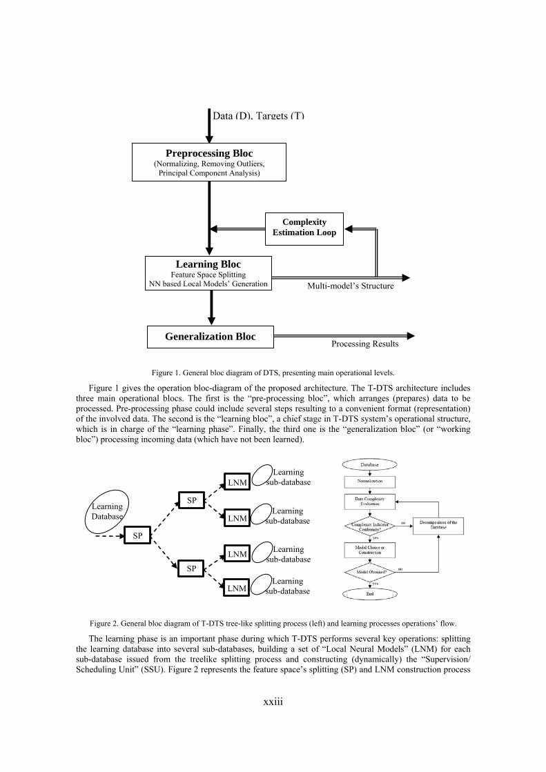
Figure 1. General bloc diagram of DTS, presenting main operational levels.

Figure 1 gives the operation bloc-diagram of the proposed architecture. The T-DTS architecture includes three main operational blocs. The first is the “pre-processing bloc”, which arranges (prepares) data to be processed. Pre-processing phase could include several steps resulting to a convenient format (representation) of the involved data. The second is the “learning bloc”, a chief stage in T-DTS system’s operational structure, which is in charge of the “learning phase”. Finally, the third one is the “generalization bloc” (or “working bloc”) processing incoming data (which have not been learned).

LNM

LNM

LNM

SP

SP

LNM

Learning Database

SP

Learning sub-database




Figure 2. General bloc diagram of T-DTS tree-like splitting process (left) and learning processes operations’ flow.

The learning phase is an important phase during which T-DTS performs several key operations: splitting the learning database into several sub-databases, building a set of “Local Neural Models” (LNM) for each sub-database issued from the treelike splitting process and constructing (dynamically) the “Supervision/ Scheduling Unit” (SSU). Figure 2 represents the feature space’s splitting (SP) and LNM construction process

Processing Results

Multi-model’s Structure

Learning Bloc Feature Space Splitting

NN based Local Models’ Generation

Preprocessing Bloc (Normalizing, Removing Outliers,

Principal Component Analysis)

Data (D), Targets (T)

Generalization Bloc

Complexity Estimation Loop

xxiv

bloc diagram. As this figure shows, after the learning phase, a set of neural network based models (trained from sub-databases) are available and cover the behaviour (map the complex model) region-by-region in the problem’s feature space. In this way, a complex problem is decomposed recursively into a set of simpler sub-problems: the initial feature space is divided into M sub-spaces. For each subspace k, T-DTS constructs a neural based model describing the relations between inputs and outputs (data). If a neural based model cannot be built for an obtained sub-database, then, a new decomposition will be performed on the concerned sub-space, dividing it into several other sub-spaces. Figure 3 gives the bloc diagram of the constructed solution (e.g. constructed multi-model). As shows this figure, the issued processing system appears as a multi-model including a set of local models and a supervision unit (e.g. SSU). When processing an unlearned data, first the SSU determines the most suitable LMN for processing that incoming data; then, the selected LMN processes the data.

Output-1

Input

Control Path

Data Path

LNM k

LNM M

LNM 1

Supervisor Scheduler

Unit

Output-k

Output-M

Y1

Yk

YM ( )tΨ

Figure 3. General bloc diagram of T-DTS generalization phase

Complexity estimation

methods

Bayes error estimation

Space partitioning

Class Discriminability Measures (Kohn, 1996)Purity measure (Singh, 2003) Neighborhood Separability (Singh, 2003) Collective entropy (Singh, 2003)

Indirect

Chernoff bound (Chernoff, 1966) Bhattacharyya bound (Bhattacharya, 1943) Divergence (Lin, 1991) Mahalanobis distance (Takeshita, 1987) Jeffries-Matusita dist. (Matusita, 1967) Entropy measures (Chen, 1976)

Non-parametric

Error of the classifier itself k-Nearest Neighbours, (k-NN) (Cover et al.,1967) Parzen Estimation (Parzen, 1962) Boundary methods (Pierson, 1998)

Other

Correlation-based approach (Rahman, 2003) Fisher discriminator ratio (Fisher, 2000) Interclass distance measure (Fukunaga, 1990) Volume of the overlap region (Ho et al, 1998) Feature efficiency (Friedman et al., 1979) Minimum Spanning Tree (Ho, 2000) Inter-intra cluster distance(Maddox, 1990) Space covered by epsilon neighbourhoods Ensemble of estimators

Figure 4. Taxonomy of classification’s complexity estimation methods

“Complexity Estimation Loop” (CEL) plays a capital role in splitting process (initial complex problem’s division into a set of sub-problems with reduced complexity), proffering self-organization capability of T-DTS. It acts as some kind of “regulation” mechanism which controls the splitting process in order to handle the global task more efficiently. The complexity estimation based decomposition could be performed according to two general strategies: “static regulation policy” and “adaptive regulation policy”. In both strategies, the issued solution could either be a binary tree-like ANN based structure or a multiple branches tree-like ANN based framework. The main difference between two strategies remains in nature of the complexity estimation indicators and the splitting decision operator performing the splitting process: “static splitting policy” in the first one and “adaptive decomposition policy” in the second. Figure 4 gives the general

xxv

taxonomy of different “complexity estimation” approaches including references describing a number of techniques involved in above-mentioned two general strategies. In a general way, techniques used for complexity estimation could be sorted out in three main categories: those based on “Bayes Error Estimation”, those based on “Space Partitioning Methods” and others based on “Intuitive Paradigms”. Bayes Error Estimation” may involve two classes of approaches, known as: indirect and non-parametric Bayes error estimation methods, respectively.

Concerning on “Intuitive Paradigms” based complexity estimation, an appealing approach is to use the ANN learning as complexity estimation indicator (Budnyk et al., 2008). The idea is based on following assumption: “more complex a task (or problem) is more neurons will be needed to learn it correctly”. However, the choice of an appropriated neural model is here of major importance. In fact, the learning rule of the neural network’s model used as complexity estimator has to be sensitive to the problem’s complexity. If m represents the number of data to learn and )(mgi is a function relating the learning complexity, then a first indicator could be defined as relation (1). An adequate candidate satisfying the above-mentioned condition is the class of Kernel-like Neural Networks. In this kind of neural models the learning process acts directly on number of connected (e.g. involved) neurons in the unique hidden layer of this kind of ANN. For this class of ANN, gi(m) could be be the number of needed neurons in order to achieve a correct learning of m data, leading to a simple form of relation (1), expressed in term of relation (2) where n is the number of connected neurons in the hidden layer.

mmg

mQ ii

)()( = 0)(,1, ≥≥ mgm i (1)

mnQ = , 0,1 ≥≥ nm (2)

An appealing simple version of kernel-like ANN is implemented by the IBM ZISC-036 neuro-processor (Detremiolles, 1998). In this simple model a neuron is an element, which is able to:

• memorize a prototype (64 components coded on 8 bits), the associated category (14 bits), an influence field (14 bits) and a context (7 bits),

• compute the distance, based on the selected norm (norm L1 or LSUP) between its memorized prototype and the input vector (the distance is coded on fourteen bits),

• compare the computed distance with the influence fields, • communicate with other neurons (in order to find the minimum distance, category, etc.), • adjust its influence field (during learning phase).

The ZISC-036 learning mechanism’s simplicity make it a suitable candidate for implementing the above-described intuitive complexity estimation concept.

2.2 Software Implementation T-DTS software incorporates three databases: decomposition methods, ANN models and complexity estimation modules T-DTS software engine is the Control Unit. This core-module controls and activates several software packages: normalization of incoming database (if it’s required), splitting and building a tree of prototypes using selected decomposition method, sculpting the set of local results and generating global result (learning and generalization rates). T-DTS software can be seen as a Lego system of decomposition methods, processing methods powered by a control engine an accessible by operator thought Graphic User Interface. The current T-DTS software (version 2.02) includes the following units and methods: - Decomposition Units:

CN (Competitive Network) SOM (Self Organized Map) LVQ (Learning Vector Quantization)

- Processing Units: LVQ (Learning Vector Quantization) Perceptrons MLP (Multilayer Perceptron) GRNN (General Regression Neural Network) RBF (Radial basis function network) PNN (Probabilistic Neural Network) LN

xxvi

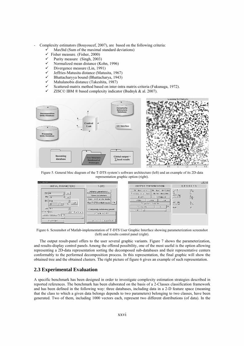
- Complexity estimators (Bouyoucef, 2007), are based on the following criteria: MaxStd (Sum of the maximal standard deviations) Fisher measure. (Fisher, 2000) Purity measure (Singh, 2003) Normalized mean distance (Kohn, 1996) Divergence measure (Lin, 1991) Jeffries-Matusita distance (Matusita, 1967) Bhattacharyya bound (Bhattacharya, 1943) Mahalanobis distance (Takeshita, 1987) Scattered-matrix method based on inter-intra matrix-criteria (Fukunaga, 1972). ZISC© IBM ® based complexity indicator (Budnyk & al. 2007).

Figure 5. General bloc diagram of the T-DTS system’s software architecture (left) and an example of its 2D-data

representation graphic option (right).

Figure 6. Screenshot of Matlab-implementation of T-DTS User Graphic Interface showing parameterization screenshot (left) and results control panel (right).

The output result-panel offers to the user several graphic variants. Figure 7 shows the parameterization, and results-display control panels Among the offered possibility, one of the most useful is the option allowing representing a 2D-data representation sorting the decomposed sub-databases and their representative centers conformably to the performed decomposition process. In this representation, the final graphic will show the obtained tree and the obtained clusters. The right picture of figure 6 gives an example of such representation.

2.3 Experimental Evaluation

A specific benchmark has been designed in order to investigate complexity estimation strategies described in reported references. The benchmark has been elaborated on the basis of a 2-Classes classification framework and has been defined in the following way: three databases, including data in a 2-D feature space (meaning that the class to which a given data belongs depends to two parameters) belonging to two classes, have been generated. Two of them, including 1000 vectors each, represent two different distributions (of data). In the

xxvii

first database, data is distributed according to “circle” geometry (symmetrical). In the second database, data is distributed conformably to a two spirals-like geometry. Each database has been divided into two equal parts (learning and generalization databases) of 500 vectors each. Databases are normalized (to obtain mean equal to 0 and variance equal to 1). The third database contains a set of data distributions (databases generated according to a similar philosophy that for the previous ones) with gradually increasing classification difficulties. Figure 7 gives three examples of data distributions with gradually increasing classification difficulty: (1) corresponds to the simplest classification problem and (12) the most difficult.

(1) (6) (12)

Figure 7. Benchmark: databases examples with gradually increasing complexity.

50%

60%

70%

80%

90%

100%

1 2 3 4 5 6 7 8 9 10 11 12Problem ref erence

rate

(%)

0,0

20,0

40,0

60,0

80,0

100,0

Tim

e (s

)

Learning Rate %Generalization Rate %Time (s)

Fishe r = 0 .7 5

50%

60%

70%

80%

90%

100%

1 2 3 4 5 6 7 8 9 10 11 12Problem reference

rate

(%)

0

20

40

60

80

100

Tim

e (s

) / P

U

Learn. RateGener. RatePUTime (s)

Figure 8. Results for modular structure with static complexity estimation strategy (left) and adaptive complexity

estimation strategy (right). Time” corresponds to the “learning phase” duration and PU to “number of generated local models”.

Based on the above-presented set of benchmark problems, two self-organizing modular systems have been generated in order to solve the issued classification problem. The first one using the “static” complexity estimation method with a threshold based decomposition decision rule, and the second one, using “adaptive” complexity estimation criterion based on Fisher’s decimator. As the Fisher’s discriminator based complexity estimation indicator measures distance between two classes (versus the averages and dispersions of data representative of each class), it could be used to adjust the splitting decision proportionally to problem’s difficulty: a short distance between two classes (of data) reflects higher difficulty, while, well separated classes of data delimit two well identified regions (of data), and thus, lower processing complexity. Figures 8 gives classification results obtained for each of the above-considered case. One can note from the left diagram of figure 8, that the processing times are approximately the same for each dataset. While, the classification rate drops significantly for more complicated datasets. That proves that the when databases complexity is increasing such modular system cannot maintain the processing quality. Concerning figure 9, as one can notice, significant enhancement in generalization phase. The classification rates for learning mode are alike, achieving good learning performance. In fact, in generalization (test) phase, there is only a small dropping tendency of the classification rate when the classification’s difficulty increases. However, in this case, processing time (concerning essentially the learning phase) increases significantly for more complex datasets. This fact is in contrast with results obtained for the previous structure (results presented in the right diagram of figure 8). In fact, in this case dynamic structure adapts decomposition (and so, the modularity) in order to reduce processing complexity, by creating a processing modular structure proportional to the processed data’s complexity.

xxviii

Figure 9. Number of generated models versus the splitting threshold for each complexity estimation technique: results

obtained for “circular” distribution (a) and ”two spiral” distribution (b) respectively.

Extending the experiment to other complexity estimation indicators, similar results have been obtained for different indicators with more or less sensitivity. Figures 9 gives the number of generated models versus the splitting threshold for each complexity estimation technique for “circular” and ”two spiral” distributions respectively. For both databases the best classification rate was obtained when the decomposition (splitting) is decided using “purity” measurement based complexity indicator. However, at the same time, “Fisher’s” discriminator based complexity estimation achieved performances close to the previous one. Regarding the number of generated models, the first complexity estimation indicator (purity) leads to much greater number of models.

Figure 10. ZISC-036 neuro-computer based complexity indicator versus the learning database’s size (m).

Table 2. Correct classification rates within different configurations: T-DTS with different complexity estimators. Gr represents “correct classification rate”, Std. Dev. is “standard deviation”, “TTT” abbreviates the Tic-tac-toe end-game

problem and “DNA” abbreviates the second benchmark. LGB is the data fraction (in %) used in learning phase and GDB is the data fraction used in generalization phase.

Experimental Conditions Complexity Estimator used in T-DTS Max Gr (± Std. Dev.) (%) TTT with LGB = 50% & GDB = 50% Mahalanobis com. est. 84.551 (± 4.592) TTT with LGB = 50% & GDB = 50% ZISC based com. est. 82.087 (± 2.455) TTT with LGB = 50% & GDB = 50% Normalized mean com. est. 81.002 (±1.753) DNA with LGB = 20% & GDB = 80% Mahalanobis com. est. 78.672 (± 4.998) DNA with LGB = 20% & GDB = 80% Jeffries-Matusita based com. est. 75.647 (±8.665) DNA with LGB = 20% & GDB = 80% ZISC based com. est. 80.084 (± 3.176)

Finally, a similar verification benchmark including five increasing levels of complexity (resulting in “Q1”

to “Q5” different sets of Qi indicator’s values: Q1 corresponds to the easiest one and Q5 to hardest problem) and eight different databases’ sizes, indexed from “1” to “8” respectively (containing 50, 100, 250, 500, 1000,

xxix

2500, 5000 and 10000 patterns respectively), has been carried out. For each set of parameters, tests have been repeated 10 times in order to get reliable statistics in order to check the obtained results’ deviation and average. Totally, 800 tests have been performed. Figure 11 gives the evaluation results within the above-described experimental protocol. The expected behavior of Qi indicator could be summarized as follow: for a same problem (e.g. same index) the increasing of number of representative data (e.g. m parameter) tends to decrease the indicator’s value (e.g. the enhancement of representatively reduces problem’s ambiguity). On the other hand, for problems of increasing complexity, Qi indicator tends to increases its value. I, fact, as one can remark from Figure 11, the proposed complexity estimator’s value decreases when the learning database’s size increases. In the same way, the value of the indicators ascends from easiest classification task (e.g. Q1) to the hardest one (e.g. Q5). The results of figure 5 show that the proposed complexity estimator is sensitive to the classification task’s complexity and behaves conformably to the aforementioned expectations.

In order to extend the frame of the evaluation tests, two patterns classification benchmark problems have been considered. The first one, known as “Tic-tac-toe end-game problem” where the goal consists of predicting whether each of 958 legal endgame boards for tic-tac-toe is won for `x'. The 958 instances encode the complete set of possible board configurations at the end of tic-tac-toe. This problem is hard for the covering family algorithm, because of multi-overlapping. The second one, known as “Splice-junction DNA Sequences classification problem”, aims to recognize, given a sequence of DNA, the boundaries between exons (the parts of the DNA sequence retained after splicing) and introns (the parts DNA of the sequence that are spliced out). This problem consists of two subtasks: recognizing exon/intron boundaries (referred to as EI sites), and recognizing intron/exon boundaries (IE sites). There are 3190 numbers of instances from Genbank 64.1, each of them compound 62 attributes which defines DNA sequences (ftp-site: ftp://ftp.genbank.bio.net) problem. Table 1 gives the obtained results for different configurations, T-DTS with different complexity estimators. It is pertinent to emphasize the relative stability of the “correct classification rates” and the corresponded “standard deviations” when intuitive ANN based complexity estimator is used.

3. CONCLUSION

A key point on which one can act is the processing complexity reduction. It may concern not only the problem representation’s level (data) but also may appear at processing procedure’s level. An issue could be processing model complexity reduction by splitting a complex problem into a set of simpler sub-problems: multi-modeling where a set of simple models is used to sculpt a complex behavior.

The main goal of this paper was to show that by introducing “modularity” and “self-organization” ability obtained from “complexity estimation based regulation” mechanisms, it is possible to obtain powerful adaptive modular information processing systems carrying out higher level intelligent operations. Especially, concerning the classification task, a chief steps in data-mining process, the presented concept show appealing potentiality to defeat ever-increasing needs of nowadays complex data-mining applications.

ACKNOWLEDGEMENT

I would like to express my gratitude to Dr. Abrennasser Chebira, member of my research team who have engaged his valuable efforts since 1999 on this topic. I would also express many thanks to Dr. Mariusz Rybnik and Dr. El-Khier Bouyoucef, who have strongly contributed in carried out advances with in their PhD thesis. Finally, I would like thank Mr. Ivan Budnyk my PhD student who actually works on T-DTS and intuitive complexity estimator.

REFERENCES

Book Author, year. Title (in italics). Publisher, location of publisher. Abiteboul, S. et al, 2000. Data on the Web: From Relations to Semistructured Data and XML. Morgan Kaufmann

Publishers, San Francisco, USA.

xxx

Journal Author, year. Paper title. Journal name (in italics), volume and issue numbers, inclusive pages. Bodorik P. et al, 1991. Deciding to Correct Distributed Query Processing. In IEEE Transactions on Data and Knowledge

Engineering, Vol. 4, No. 3,pp 253-265. Conference paper or contributed volume Author, year, paper title. Proceedings title (in italics). City, country, inclusive pages. Beck, K. and Ralph, J., 1994. Patterns Generates Architectures. Proceedings of European Conference of Object-Oriented

Programming. Bologna, Italy, pp. 139-149. Bhattacharya A., 1943, On a measure of divergence between two statistical populations defined by their probability

distributions, Bulletin of Calcutta Maths Society, vol. 35, pp. 99-110. Budnyk I., Bouyoucef E., Chebira A., Madani K., 2008, Neuro-computer Based Complexity Estimator Optimizing a

Hybrid Multi-Neural Network structure, COMPUTING, ISSN 1727-6209, Vol.7, Issue 3, pp. 122-129. Chen C.H., 1976, On information and distance measures, error bounds, and feature selection, Information Sciences, pp.

159-173. Chernoff A., 1966, Estimation of a multivariate density, Annals of the Institute of Statistical Mathematics, vol. 18, pp.

179-189. Cover T. M., Hart P. E., 1967, Nearest neighbors pattern classification, IEEE Trans on Inform. Theory, Vol. 13, pp.21-27. De Tremiolles G., 1998, Contribution to the theoretical study of neuro-mimetic models and to their experimental

validation: a panel of industrial applications, Ph.D. Report, University of PARIS 12, (in French) Fisher A., 2000, The mathematical theory of probabilities, John Wiley. Friedman J. H.,. Rafsky L. C, 1979, Multi-variate generalizations of the Wald-Wolfowitz and Smirnov two sample tests,

The Annals of Statistics, Vol. 7(4), pp. 697-717. Fukunaga K.., 1990, Introduction to statistical pattern recognition, Academic Press, New York, 2nd ed.. Ho K. , Baird H. S., 1993, Pattern classification with compact distribution maps, Computer Vision and Image

Understanding, Vol. 70(1), pp. 101-110. Ho T. K., 2000, Complexity of classification problems and comparative advantages of combined classifiers, Lecture Notes

in Computer Science. Kohn A., Nakano, L.G., and Mani V., 1996, A class discriminability measure based on feature space partitioning, Pattern

Recognition, 29(5), pp. 873-887 Lin J., 1991, Divergence measures based on the Shannon entropy”, IEEE Transactions on Information Theory, 37(1):145-

151. Madani K., Chebira A., Rybnik M., 2003 - a. Data Driven Multiple Neural Network Models Generator Based on a Tree-

like Scheduler, LNCS "Computational Methods in Neural Modeling", Ed. J. Mira, J.R. Alvarez - Springer Verlag 2003, ISBN 3-540-40210-1, pp. 382-389.

Madani K., Chebira A., Rybnik M., 2003 - b. Nonlinear Process Identification Using a Neural Network Based Multiple Models Generator, LNCS "Computational Methods in Neural Modeling", Ed. J. Mira, J.R. Alvarez - Springer Verlag 2003, ISBN 3-540-40211-X, pp. 647-654.

Madani K., Thiaw L., Malti R., Sow G., 2005 - a. Multi-Modeling: a Different Way to Design Intelligent Predictors, LNCS, Ed. J. Cabestany, A. Prieto and D.F. Sandoval - Springer Verlag, Vol. 3512, pp. 976-984.

Madani K., Chebira A., Rybnik M., Bouyoucef E., 2005 - b. Intelligent Classification Using Dynamic Modular Decomposition, 8-th International Conference on Pattern Recognition and Information Processing (PRIP 2005), May 18-20, 2005, Minsk, Byelorussia, ISBN 985-6329-55-8, pp. 225-228.

Matusita K., 1967, On the notion of affinity of several distributions and some of its applications, Annals Inst. Statistical Mathematics, Vol. 19, pp. 181-192.

Parzen E., On estimation of a probability density function and mode, Annals of Math. Statistics, vol. 33, pp. 1065-1076. Pierson W.E., 1998, Using boundary methods for estimating class separability, PhD Thesis, Dept of Elec. Engin, Ohio

State University. Rahman A. F. R., Fairhurst M., 1998, Measuring classification complexity of image databases: a novel approach, Proc of

Int Conf on Image Analysis and Processing, pp. 893-897. Singh S., 2003, Multi-resolution estimates of classification complexity, IEEE Trans on Pattern Analysis and Machine

Intelligence Takeshita T., Kimura F., Miyake Y., 1987, On the estimation error of Mahalanobis distance, Trans. IEICE, pp. 567-573.

Full Papers

AN EXPERIMENTAL STUDY OF THE DISTRIBUTED CLUSTERING FOR AIR POLLUTION PATTERN

RECOGNITION IN SENSOR NETWORKS

Yajie Ma Information Science and Engineering College, Wuhan University of Science and Technology

947, Heping Road, Wuhan, 43008, China Department of Computing, Imperial College London

180 Queens Gate, London, SW7 2BW, UK

Yike Guo, Moustafa Ghanem Department of Computing, Imperial College London

180 Queens Gate, London, SW7 2BW, UK

ABSTRACT

In this paper, we make an experimental study of the urban air pollution pattern analysis within MESSAGE system. A hierarchical network framework consisted of mobile sensors and stationary sensors is designed. A sensor gateway core architecture is developed which is suited to grid-based computation. Then we make experimental analysis including the identification of pollution hotspots and the dispersion of pollution clouds based on a real-time peer-to-peer clustering algorithm. Our results provide a typical air pollution pattern in urban environment which gives a real-time track of the air pollution variation.

KEYWORDS

Pattern recognition, Distributed clustering, Sensor networks, Grid, Air pollution.

1. INTRODUCTION

Road traffic makes a significant contribution to the following emissions of pollutants: benzene(C6H6), 1,3~butadiene, carbon monoxide(CO), lead, nitrogen dioxide(NO2), Ozone(O3), particulate matter(PM10 and PM2.5) and sulphur dioxide(SO2). In the past decade, environmental applications including air quality control and pollution monitoring [1–3] are experiencing a steadily increasing attention. Under the current Environment Act of UK [4], most local authorities have air quality monitoring stations to provide environmental information to public daily via Internet. The conventional approach to assessing pollution concentration levels is based on data collected from a network of permanent air quality monitoring stations. However, permanent monitoring stations are frequently situated so as to measure ambient background concentrations or at potential ‘hotspot’ locations and are usually several kilometers apart. According to our earlier research of ‘Discovery Net EPSRC e-Science Pilot Project’ [5], we learnt that the pollution levels and the hot spots change with time. This kind of pollution levels and hot spots change can be calculated as dispersion under some sets of meteorology conditions. Whatever dispersion model is used, it should relate to the source, meteorology, and spatial patterns to air quality at receptor points [6]. Till now, much attention has been paid to the spatial patterns in relationships between sources and receptors, such as how the arrangement of sources affects the air quality at receptor locations [7], how to employ various kinds of atmospheric pollution dispersion models [8, 9], and etc. However, the phenomenon of road traffic air pollution shows considerable variation within a street canyon as a function of distance to the source of pollution [10]. Therefore, the levels and consequently the effected number of inhabitants vary. Information on a number of key factors such as individual driver/vehicle activity, pollution concentration and individual human exposure has traditionally either simply not been available or only available at high levels of spatial and temporal

IADIS European Conference Data Mining 2009

3

aggregation This is mainly caused by the critical data gaps and asymmetries in data coverage, as well as the lack of on-line data processing capability offered by the e-Science.

We can fill these data gaps by two ways: generating new forms of data (e.g., on exposure and driver/vehicle activity) and generating data at higher levels of spatial and temporal resolution than existing sensor systems. Taking advantage of the low cost mobile environmental sensor system, we construct the MESSAGE (Mobile Environmental Sensor System Across Grid Environments) system[11], which fully integrates existing static sensor systems and complementary data sources with the mobile environmental sensor system. It can provide radically improved capability for the detection and monitoring of environmental pollutants and hazardous materials.

In this paper, based on our former work of MoDisNet [12], we introduce the experimental analysis for urban air pollution monitoring within the MESSAGE system. The main contributions of this paper are: first, we propose a sensor gateway core architecture for sensor grid to provides the processing, integrating, and analyzing heterogeneous sensor data in both centralized and distributed ways. With the support of the hierarchical network architecture formed by the mobile sensors fixed by the roadside devices and stationary sensors carried by the public vehicles, the MESSAGE system fully considers the urban background and the pollution features, which is highly effective for air pollution monitoring. Second, we make an experimental study for typical air pollution pattern analysis in urban environment based on a solution of the real-time distributed clustering algorithm in sensor grid, which gives a real-time track of the air pollution variation. The results also present important information about environmental protection and individual super vision.

In the remainder of this paper, we first present the system architecture to meet the demands of the project in section 2. We also discuss the novel techniques we provide to address the problems when a sensor grid is constructed based on the mobile and high-throughput real-time data environment. In section 3, the distributed clustering algorithm is introduced as well as the performance analysis. We describe the real-time pollution pattern recognition experiments in section 4. Section 5 concludes the paper with a summary of the research and a discussion of future work.

2. METHODOLOGY

2.1 Modeling Approach

The key feature of the MESSAGE system is to use a variety of vehicle fleets including buses, service vehicles, taxis and commercial vehicles as platform for environmental sensors. With the collaboration of the static sensors fixed on roadside, the whole system can detect the real-time air pollution distribution in London. To satisfy this demand, the MESSAGE system is constructed based on a two-layer network architecture cooperating with the e-Science Grid architecture. The Grid structure is featured by the sensor gateway core architecture, which enables the sensors themselves naturally form and communicate with each other in P2P style within large scale mobile sensor networks. These will provide MESSAGE with the ability to support the full scale analytical task ranging from dynamic real time mining of sensor data to the analysis of off-line data warehoused for historical analysis. The sensors in MESSAGE Grid are equipped with sufficient computational capabilities to participate in the Grid environment and to feed data to the warehouse as well as perform analysis tasks and communicating with their peers.

The network framework and the sensor gateway core architecture are illustrated in Figure 1(a) and (b). The mobile sub-network formed by the Mobile Sensor Nodes (MSN in short) and the stationary sub-

network organized by the Static Sensor Nodes (SSN in short). MSNs are installed in the vehicles. They sample the pollution data and execute the AD conversion to get the digital signals. According to the system requirements, the MSNs may pre-process the raw data (such as the noise reduction, local data cleaning and fusion, etc.) and then send these data to a nearest SSN. The SSNs take in charge of the data receiving, update, storage and exchange works.

The sensors (including SSN and MSN) connect to the MESSAGE Grid by several Sensor Gateways (SGs) according to different wireless access protocols. The sensors are capable of collecting the air pollution data up to 1Hz frequency and sending the data to the remote Grid service hop by hop. This capability enable the sensors exchange their raw data locally and then realize the data analysis and mining in distributed way.

ISBN: 978-972-8924-88-1 © 2009 IADIS

4

The SGs take in charge of connecting the wireless sensor network with the IP backbone, which can be either wired or wireless. All SGs are managed by a Root Gateway (RG), which is a logical entity that may consist of a number of physical root nodes that operate in a peer-to-peer environment to ensure reliability. The RG is the central element of the Sensor Gateway architecture. The SG Service maintains details of the SGs that are available and their available capacity. The aim of RGs is to load-balance across the available SGs, which is very useful for improving the throughput and performance of the Grid architecture. A database that can be accessed by SQL is managed by the Grid architecture which centrally stores and maintains all the archived data, including derived sensor data and the third part data such as the traffic data, the weather data and the health data. These data can provide wealth of information for the Grid computation to generate the short-term or long-term models that relate to the air pollution and traffic. Furthermore, it may give the supervision for the prediction of the forthcoming events about the traffic change and pollution trend.

Mobile Sensor Node (MSN)

Static Sensor Node (SSN)

Roo

t Gat

eway

P

rovi

sion

sSe

nsor

Gat

eway

Dat

a flo

w

from

pai

red

sens

ors

Dat

a flo

w

from

pai

red

sens

ors

Dat

a flo

w fr

om

sens

ors

to

paire

d se

nsor

G

atew

ay

(a) network framework (b) sensor gateway core architecture

Figure 1. The Network Framework and Sensor Gateway Core Architecture within MESSAGE

2.2 Preparation of Input Data

The input data based on our former research [5] uses the air pollution data sampled from 140 sensors marked as the red dots (see Figure 3 and 4 in section 4) distributed in a typical urban area around the Tower Hamlets and Bromley areas in east London. There are some of the typical landmarks such as the main roads extending from A6 to L10 and M1 to K10, the hospitals around B5 and K4, the schools at B7, C8, D6, F10, G2, H8, K8 and L3, the train stations at D7 and L5, and a gas work between D2 and E1. 140 sensors collect data from 8:00 to 17:59 at 1-minute intervals to monitor the pollution volumes of NO, NO2, SO2 and Ozone. Then there are 600 data items for each node and totally 84000 data items for the whole network. Each data item is identified by a time stamp, a location, and a four-pollutant volume reading. Once sensor data is collected, data cleaning and preprocessing is necessary before further analysis and visualization can be performed. Most importantly, missing data must be performed using bounding data from the sensor, or also using data from nearby sensors at the same time. Interpolated data may be stored back to the original database, with provenance information including the algorithm used. Such pre-processing is standard, and has been conducted using the available MESSAGE component. The relatively high spatial density of sensors used also allows a detailed map of pollution in both space and time to be generated.


5

3. DISTRIBUTED CLUSTERING ALGORITHM

Data mining for pollution monitoring in sensor networks in urban environment faces several challenges. First, the methods of data collection and pre-processing highly rely on the complexity of the environment. For example, the distribution and features of pollution data are correlated to inter-relationships between the environment, geography, topography, weather and climate and the pollution source, which may guide the design of the data mining algorithms. Also, the mobility of the sensor nodes increases the complexity of sensor data collection and analysis [13, 14]. Second, resource-constrained (power, computation or communication), distributed and noisy nature of sensor networks presents challenges for storing the historical data in each sensor, even for storing the summary/pattern from the historical data [15]. Third, sensor data come in time-ordered streams over network, which makes traditional centralized mining techniques inapplicable. As the result, the real-time distributed data mining (DDM in short) schemes are significantly demanded in such scenario. Considering the pattern recognition application, in this section, we introduce a peer-to-peer clustering algorithm as well as the performance analysis.

3.1 P2P Clustering Algorithm

To realize the DDM algorithm with the capability to provide the information exchange in P2P style, a P2P clustering algorithm is designed to find out the pollution patterns in the urban environment according to the sampled air pollutants’ volumes. The algorithm is a hierarchical clustering algorithm based on DBSCAN in [16]. However, our algorithm has the following characteristics:

1. Nodes only require local synchronization at any time, which is better suited to a dynamic environment. 2. Nodes only need to communicate with their immediate neighbors, which reduces the communication

complex. 3. Data are inherently distributed in all the nodes, which makes the algorithm be widely used in large,

complex systems. The algorithm runs in each SSN (MSN only takes in charge of collecting data and sending data to a

closest SSN). In order to describe this algorithm, we give some definitions first (suppose the total numbers of SSN is n (n > 0)).

SSNi: a SSN node with the identity i (i = 0, …, n-1); Si: an Information Exchange Node Set (IENS) of SSNi, which is a set of some of the SSNs that can

exchange information with SSNi; CS: candidate cluster centre set. Each element in CS is a cluster centre; Cl

i,j: the cluster center of jth (j ≥ 0) cluster that is computed in SSNi in lth recursion (l ≥ 0), Cli,j∈CS;

Numi,j: the number of members (data points) belongs to jth cluster in SSNi; E(X, Y): the Euclidian distance of data X and Y; D: a pre-defined distance threshold; δ: a pre-defined offset threshold. The algorithm proceeds as follows. 1. Generates Si and local data set. Node SSNi receives data from MSNs as local data and chooses a

certain number of SSNs as Si in term of a random algorithm (the detail of the random algorithm is beyond the scope of this article).

2. Generates CS. This process is described by the following pseudo code: SSNi chooses a data item j from its local data set into CS as C0

i,j; for each other data item k in the local data set of SSNi

for each data item m ∈ CS if E(k, m)>D put k into CS as C0

i,k; 3. Distributes data. For each candidate cluster centre C0

i,j∈CS and a data item Y, if E(C0i,j, Y) < D, then

distribute Y into the cluster. Thus each local cluster of SSNi can be described as (C0i,j, Numi,j)

4. Updates CS. Node SSNi exchanges local data description with all the nodes in Si. After SSNi receives all the data descriptions it wants, it checks to see if two cluster centres C0

i,j, C0i,k satisfy E(C0

i,j, C0i,k) < 2D,

then it combines these two clusters and updates the cluster centre as C1i,j.

ISBN: 978-972-8924-88-1 © 2009 IADIS

6

5. Compares C0i,j and C1

i,j. Computes the offset between C1i,j and C0

i,j. If the offset ≤ δ, then the algorithm finishes; otherwise SSNi replaces C0

i,j with C1i,j, and go to step 3.

3.2 Clustering Accuracy Analysis

The evaluation of the accuracy of the algorithm aims to investigate in what degree our P2P clustering algorithm can assign the data items into the correct clusters in comparison with the centralized algorithm. To do so, we design an experimental environment for data exchange and algorithm execution. The network topology of the simulation is shown in Figure 2. We use 18 sensor nodes, including 12 SSN nodes from node 0 to node 11 and 6 MSN nodes from node 12 to node 17. Data are sampled at each MSN and sent to a nearest SSN. The air pollution data we use is consisted of the volumes of four pollutants NO, NO2, SO2, and O3 sampled at 1-minute intervals in urban environment from 8:00 to 17:59 within a day collected from 6 MSNs (as described in Section 2.2). Then, the total number of data items in the dataset is 3600. Data can be sent and received in bi-directions along the edges.

The comparison of the average clustering accuracy of the centralized and distributed clustering algorithms is shown in Table 1. For the centralized clustering algorithm, we suppose node 8 be the sink (central point for data processing), which means every other MSN sends the data to node 8. And the classic DBSCAN algorithm is running in node 8 for centralized clustering. For the accuracy measurement, let iX denote the dataset at node i. Let )(xLi

km and )(xLi denote the labels (cluster membership) of sample x ( iXx∈ ) at node i under centralized DBSCAN algorithm and our distributed clustering algorithm respectively. We define the Average Percentage Membership Match (APMM) as

∑=

×=∈

=n

ii

ikm

ii

XxLxLXx

nAPMM

1%100

|||)}()(:{|1 (1)

Where n is the total number of SSNs. For the distributed clustering algorithm, we vary the number of nodes in the Information Exchange Node

Set (IENS) of each SSN from 1 to 10. Let D = 10 and δ = 1. Data are randomly assigned to each SSN. Table 1 shows the APMM results.

0123

4567

891011

12

1314

15

16

17

Figure 2. The Network Topology of the Simulation

Table 1. Centralized Clustering vs. Distributed Clustering (APMM results)

IENS 1 2 3 4 5 6 7 8 9 10 APMM 86.3% 91.2% 92.67% 93.46 93.55% 93.74% 93.93% 94.23% 94.59% 94.97%

From Table 1 we can see that, when the number of nodes in IENS is no less than 2, in other words, when each SSN exchanges data with at least two other SSNs, the APMM exceeds 91%. When the number of nodes in IENS is no less than 4, the APMM exceeds 93%. The results are achieved under the condition of assigning the data to each SSN randomly. In reality, if the patterns of the dataset are various in different locations, the APMM may be lower than the results in Table 1. In such situations, a good scheme of how to choose the nodes to construct the IENS would be very important.


7

4. EXPERIMENTAL ANALYSIS OF PATTERN RECOGNITION

4.1 Pollution Hotspots Identification

The pollution hotspots identification uses the air pollution data to find out the distribution of some key pollution locations within the research area. Our former work in Discovery Net can only classify the pollution data into several pollution levels, such as high or low, but can’t tell us the distribution of different pollutants in different locations and their contributions to the pollution levels. To improve the data analysis capability, in this data analysis experiment, we use the distributed clustering algorithm to cluster the pollutants into groups which can recognize different pollution patterns. From the experimental results of Discovery Net, we pickup all the high pollution level locations in the research area at 15:30 and 17:00 respectively to check the contribution of different pollutants (NO, NO2, SO2 and Ozone) to the pollution levels. The results are shown in Figure 3.

In this figure, different clusters/patterns correspond to different colors, which reveal the relationship between the combination and volumes of different pollutants. According to the clustering result, we use red color to denote the pattern of high volume of NO2 and Ozone whilst low volume of NO; blue color features the pattern of high volume of SO2 and Ozone; yellow color only contains high volume of SO2. From the figures we can see, at 15:30 the hotspots are located at the schools (which are highlighted by circles and almost all featured by high volume of NO2 and Ozone) and the gas work (which is highlighted by square and featured by high volume of SO2). At 17:00, the hospitals (highlighted by the ellipses) and the gas work all contribute to the pollutant of SO2.

Another kind of hotspot located on the main roads. However, they present different patterns at different time on different roads. Main road A6-L10 is covered in blue at 15:30 while red at 17:00. There are two reasons for this circumstance. First, the road transport sector is the major source of NOX emissions and the solid fuel and petroleum products are two main contributors of SO2. Second, NO2 and Ozone are all formed through a series of the photochemical reactions featuring NO, CO, hydrocarbons and PM. Generating NO2 and Ozone needs to take a period of time. This is why the density of NO2 is always high on the main road whereas Ozone at 17:00 is higher than that at 15:30. Another interesting fact is that, at 17:00 main roads A6-L10 and M1- K10 show different pollution patterns. From the figure we can see, the pollution pattern on M1-K10 is very similar to the patterns at the gas work and hospital areas, but not similar to the pattern on the other main road. We investigated this area and found that, a brook flows along this area in the near east and a factory area locates on the opposite side of the brook which is beyond the scope of this map. This can explain why the pollution patterns are different on these two main roads.

15:30 17:00

Figure 3. Pollution Hotspots Identification

ISBN: 978-972-8924-88-1 © 2009 IADIS

8

4.2 Pollution Clouds Dispersion Analysis

In this experiment, we investigate the dispersion of different pollution clouds to see their movements and changes. We pick up the pollutants of NOX (NO+ NO2) and SO2 respectively and calculate the pollution clouds of them at the time points of 17:15, 17:30 and 17:45. The results are shown in Figure 4(a) and (b).

According to the environmental reports of the UK, it is always the worst pollution distribution time period within a day after 17:00. The road transport sector contributes more than 50% to the total emission of NOX, especially in urban areas. At the meantime, the factories are another emission source of the nitride pollutants. Besides the major source of SO2 generated by the solid fuel and the petroleum products from the transport emission, some other locations such as the hospitals contribute some kind of pollutants, including the sulphide and nitride. These features are well illustrated by Figure 4.

In Figure 4(a), the main road A6-L10 and its circumjacent areas are severely covered by high volume of NOX. The same situation appears in the area from A1 to N2 which includes a gas work (between D2 and E1), side roads (A1 to J2), factories and parking lots (K1 to L2). And we can notice that the dispersion of the NOX clouds fades as the time goes by, especially around the main road area. However, the NOX clouds will stay for a long time in A1 to N2 area.

The dispersion of SO2 cloud in Figure 4(b), however, shows different feature. The cloud mainly covers the main roads, as well as two hospitals (around B5 and K4). In comparison with the result at 17:15, the SO2 cloud blooms at 17:30, which lays almost over all the two main roads and hospitals. However, it fades quickly at 17:45 and uncovers a lot of areas, especially the main road M1-K10 and hospital K4. This status may due to the different environmental conditions in this area (the dispersion of SO2 depends on a lot of factors such as the temperature, wind direction, humidity and air pressure, etc.). Besides, it also can be attributed to the existence of the brook in the near east – SO2 can be absorbed into water to form sulphurous acid very easily, which decreases the volume of SO2 in the air whereas increases the pollution of the water.

17:15 17:30 17:45

(a) NOX (NO+ NO2)

(b) SO2

Figure 4. Pollution Clouds Dispersion of NOX and SO2

5. CONCLUSION

In this paper, we make an experimental study of the urban air pollution pattern analysis within MESSAGE system. Our work is featured by the sensor gateway core architecture in sensor grid, which provides a


9

platform for different wireless access protocols, and the experiments of air pollution analysis based on distributed P2P clustering algorithm, which investigates the distribution of pollution hotspots and the dispersion of pollution clouds. The experimental results are useful for the government and local authorities to reduce the impact of road traffic on the environment and individuals.

We are currently extending the application case studies to monitor PM10 and finer detection (e.g. PM2.5). As addressing global warming becomes more important, there are increasing requirements for greenhouse gas emission monitoring and reduction. Information on greenhouse gases is therefore also needed for long term monitoring purposes with similar linkages to traffic and weather data to understand the contribution of traffic to environmental conditions.

ACKNOWLEDGEMENTS

This work was funded by the Engineering and Physical Sciences Research Council (EPSRC) project Mobile Environmental Sensing System Across a Grid Environment (MESSAGE), Grant No. EP/E002102/1.

REFERENCES

1. A. Vaseashta, G. Gallios, M. Vaclavikova, et al, 2007. Nanostructures in Environmental Pollutuion Detection, Monitoring, And Remediation. In Science and Technology of Advanced Materials, Vol. 8, Issues 1-2, pp. 47-59.

2. M. Ibrahim, E. H. Nassar, 2007. Executive Environmental Information System (ExecEIS). In Journal of Applied Sciences Research, Vol. 3, No.2, pp. 123-129.

3. N. Kularatna, B.H. Sudantha, 2008. An Environmental Air Pollution Monitoring System Based on the IEEE 1451 Standard for Low Cost Requirements. In IEEE Sensors Journal, Vol. 8, Issue 4, pp. 415-422.

4. Environment Act 1995. http://www.opsi.gov.uk/acts/acts1995/ukpga_19950025_en_1. 5. M. Richards, M. Ghanem, M. Osmond, et al, 2006. Grid-based Analysis of Air Pollution Data. In Ecological

Modelling, Vol.194, Issue 1-3, pp. 274-286. 6. R. J. Allen, L. R. Babcock, N. L. Nagda, 1975. Air Pollution Dispersion Modeling: Application and Uncertainty. In

Journal of Regional Analysis and Policy, Vol.5, No.1. 7. A. Robins, E. Savory, A. Scaperdas, et al, 2002. Spatial Variability and Source-Receptor Relations at a Street

Intersection. In Water, Air and Soil Pollution: Focus, Vol. 2, No. 5-6, pp. 381-393. 8. R. Slama, L. Darrow, J. Parker, et al, 2008. Meeting Report: Atmospheric Pollution and Human Reproduction. In

Environmental Health Perspectives, Vol. 116, No. 6, pp. 791-798. 9. M. Rennesson, D. Maro, M.L. Fitamant, et al, 2005. Comparison of the local-scale atmospheric dispersion model

CEDRAT with 85Kr measurements. In Radioprotection, Suppl. 1, Vol. 40, pp. S371-S377. 10. G. Wang, F. H. M. van den Bosch, M. Kuffer, 2008. Modeling Urban Traffic Air Pollution Dispersion. Proceedings

of The International Archives of the Photogrammetry, Remote Sensing and Spatial Information Sciences. Vol. XXXVII, Part B8, Beijing, China, pp.153-158.

11. MESSAGE: Mobile Environmental Sensing System Across Grid Environments. http://www.message-project.org. 12. Y. Ma, M. Richards, M. Ghanem, et al, 2008. Air Pollution Monitoring and Mining Based on Sensor Grid in London.

In Sensors, Vol. 8, pp. 3601-3623. 13. M.J. Franklin. Challenges in Ubiquitous Data Management, 2001. In Lecture Notes In Computer Science. Vol.2000,

pp. 24-31. 14. F. Perich, A. Joshi, T. Finin, et al, 2004. On Data Management in Pervasive Computing Environments. In IEEE

Transactions on Knowledge and Data Engineering, Vol. 16, No. 5, pp. 621-634. 15. Y. Diao, D. Ganesan, G. Mathur, et al, 2007. Rethinking Data Management for Storage-centric Sensor Networks.

Proceedings of The Third Biennial Conference on Innovative Data Systems Research, Asilomar, CA, USA, pp. 22-31. 16. M. Ester, H.-P. Kriegel, J. Sander, et al, 1996. A Density-Based Algorithm for Discovering Clusters in Large Spatial

Databases with Noise. Proceedings of The 2nd International Conference on Knowledge Discovery and Data Mining, Oregon, Portland, pp. 226-231.

ISBN: 978-972-8924-88-1 © 2009 IADIS

10

A NEW FEATURE WEIGHTED FUZZY C-MEANS CLUSTERING ALGORITHM

Huaiguo Fu, Ahmed M. Elmisery Telecommunications Software & Systems Group

Waterford Institute of Technology, Waterford, Ireland

ABSTRACT

In the field of cluster analysis, most of existing algorithms assume that each feature of the samples plays a uniform contribution for cluster analysis. Feature-weight assignment is a special case of feature selection where different features are ranked according to their importance. The feature is assigned a value in the interval [0, 1] indicating the importance of that feature, we call this value "feature-weight". In this paper we propose a new feature weighted fuzzy c-means clustering algorithm in a way which this algorithm be able to obtain the importance of each feature, and then use it in appropriate assignment of feature-weight. These weights incorporated into the distance measure to shape clusters based on variability, correlation and weighted features.

KEYWORDS

Cluster Analysis, Fuzzy Clustering, Feature Weighted.

1. INTRODUCTION

The Goal of cluster analysis is to assign data points with similar properties to the same groups and dissimilar data points to different groups [3]. Generally, there are two main clustering approaches i.e. crisp clustering and fuzzy clustering. In the crisp clustering method the boundary between clusters is clearly defined. However, in many real cases, the boundaries between clusters cannot be clearly defined. Some objects may belong to more than one cluster. In such cases, the fuzzy clustering method provides a better and more useful method to cluster these objects [2]. Cluster analysis has been widely used in a variety of areas such as data mining and pattern recognition [e.g.1, 4, 6]. Fuzzy c-means (FCM) proposed by [5] and extended by [4] is one of the most well-known methodologies in clustering analysis. Basically FCM clustering is dependent on the measure of distance between samples. In most situations, FCM uses the common Euclidean distance which supposes that each feature has equal importance in FCM. This assumption seriously affects the performance of FCM, so that the obtained clusters are not logically satisfying. Since in most real world problems, features are not considered to be equally important. Considering example in [17], the Iris database [9] which has four features, i.e., sepal length (SL), sepal width (SW), petal length (PL) and petal width (PW). Fig. 1 shows a clustering for Iris database based on features SL and SW, while Fig. 2 shows a clustering based on PL and PW. From Fig. 1, one can see that there are much more crossover between the star class and the point class. It is difficult for us to discriminate the star class from the point class. On the other hand, it is easy to see that Fig. 2 is more crisp than Fig. 1. It illustrates that, for the classification of Iris database, features PL and PW are more important than SL and SW. Here we can think of that the weight assignment (0, 0, 1, 1) is better than (1, 1, 0, 0) for Iris database classification.


11

Figure1. Clustering Result of Iris Database Based on Feature Weights (1, 1, 0, 0) by FCM Algorithm

Figure 2. Clustering Result of Iris Database Based on Feature Weights (0, 0, 1, 1) by FCM Algorithm

Feature selection and weighting have been hot research topics in cluster analysis. Desarbo [8] introduced the SYNCLUS algorithm for variable weighting in k-means clustering. It is divided into two stages. First it uses k-means clustering with initial set of weights to partition data into k clusters. It then determines a new set of optimal weights by optimizing a weighted mean-square. The two stages iterate until they obtain an optimal set of weights.

Huang [7] presented W-k-means, a new k-means type algorithm that can calculate variable weights automatically. Based on the current partition in the iterative k-means clustering process, the algorithm calculates a new weight for each variable based on the variance of the within cluster distances. The new weights are used in deciding the cluster memberships of objects in the next iteration. The optimal weights are found when the algorithm converges. The weights can be used to identify important variables for clustering. The variables which may contribute noise to the clustering process can be removed from the data in the future analysis.

With respect to FCM clustering, it is sensitive to the selection of distance metric. Zhao [12] stated that the Euclidean distance give good results when all clusters are spheroids with same size or when all clusters are well separated. In [13, 10], they proposed a G–K algorithm which uses the well-known Mahalanobis distance as the metric in FCM. They reported that the G–K algorithm is better than Euclidean distance based algorithms when the shape of data is considered. In [11], the authors proposed a new robust metric, which is distinguished from the Euclidean distance, to improve the robustness of FCM.

Since FCM’s performance depends on selected metrics, it will depend on the feature-weights that must be incorporated into the Euclidean distance. Each feature should have an importance degree which is called feature-weight. Feature-weight assignment is an extension of feature selection [17]. The latter has only either 0-weight or 1-weight value, while the former can have weight values in the interval [0.1]. Generally speaking, feature selection method cannot be used as feature-weight learning technique, but the inverse is right. To be able to deal with such cases, we propose a new FCM Algorithm that takes into account weight of each feature in the data set that will be clustered. After a brief review of the FCM in section 2, a number of features ranking methods are described in section 3. These methods will be used in determining FWA (feature weight assignment) of each feature. In section 4 distance measures are studied and a new one is proposed to handle the different feature-weights. In section 5 we proposed the new FCM for clustering data objects with different feature-weights.

2. FUZZY C-MEAN ALGORITHM

Fuzzy c-mean (FCM) is an unsupervised clustering algorithm that has been applied to wide range of problems involving feature analysis, clustering and classifier design. FCM has a wide domain of applications such as agricultural engineering, astronomy, chemistry, geology, image analysis, medical diagnosis, shape analysis, and target recognition [14]. Unlabeled data are classified by minimizing an objective function based on a distance measure and clusters prototype. Although the description of the original algorithm dates back to 1974 [4, 5] derivatives have been described with modified definitions for the distance measure and prototypes for the cluster centers [12, 13, 11, 10] as explained above. The FCM minimizes an objective function mJ , which is the weighted sum of squared errors within groups and is defined as follows:

ISBN: 978-972-8924-88-1 © 2009 IADIS

12

∞<<−= ∑ ∑= =mvxuXVUJ

A

n

k

n

i ikmikm 1,);,(

2

1 1 (1)

Where V= ( )cvvv ,........,, 21 is a vector of unknown cluster prototype (centers) piv ℜ∈ . The

value of iku represent the grade of membership of data point kx of set X= { }cxxx ,........,, 21 to the ith cluster. The inner product defined by a distance measure matrix A defines a measure of similarity between a data object and the cluster prototypes. A hard fuzzy c-means partition of X is conveniently represented by a matrix [ ]ikuU = . It has been shown by [4] that if 02 >−

Aik vx for all i and k, then

( )VU , may minimize mJ only, when m>1 and

( )

( )∑

∑

=

== n

k

mik

k

n

k

mik

i

u

Xuv

1

1 For ci ≤≤1 (2)

11

12

21 −

=∑

⎟⎟⎟

⎠

⎞

⎜⎜⎜

⎝

⎛

−

−= m

c

jAjk

Aik

ik

vx

vxu

Among others, Jm can be minimized by Picard iteration approach. This method minimizes Jm by initializing the matrix U randomly and computing the cluster prototypes (Eq.2) and the membership values (Eq.3) after each iteration. The iteration is terminated when it reaches a stable condition. This can be defined for example, when the changes in the cluster centers or the membership values at two successive iteration steps is smaller than a predefined threshold value.

The FCM algorithm always converges to a local minimum. A different initial guess of uij may lead to a different local minimum. Finally, to assign each data point to a specific cluster, defuzzification is necessary, e.g., by attaching a data point to a cluster for which the value of the membership is maximal [14].

3. ESTIMATING FWA OF FEATURES

In section 1 we mentioned that we propose a new clustering algorithm for a data objects with different feature-weights, which means that data with features of different FWA should be clustered. A key question that arises here is how we can determine the importance of each feature. In other words, we are about to assign a weight to each feature so that the weight of each feature determines the FWA of it.

To determine the FWA of features of a data set two major approaches can be adopted: Human-based approach and Automatic approach. In human-based approach we determine the FWA of each feature based on negotiation with an expert individual who has enough experience and knowledge in the field that is the subject of clustering. On the other hand, in automatic approach we use the data set itself to determine the FWA of its features. We will discuss more about these approaches in next lines.

Human-based approach: As is described above, in human-based approach by negotiating with an expert, we choose FWA of each feature. This approach has some advantages and some drawbacks. In some cases, using the data set itself to determine the FWA of each feature may fail to achieve the real FWA's, and human-based approach should be adopted to determine the FWA of each feature. Fig.3 demonstrates a situation this case happens.

Figure 3. Data Object with Two Features

Sample Data objects

012345

0 1 2 3 4 5Feature A

Feat

ure

B

For ci ≤≤1 , nk ≤≤1 (3)


13

Suppose Fig.3 shows a data objects in which FWA of feature A is two times FWA of feature B in reality. Since automatic approach uses the position of data points in the data space to determine the FWA of features, using data set itself to determine the FWA of features A and B (automatic approach) will lead to equal FWA's for A and B. Although this case (data set with homogeneously and equidistantly distributed data points) rarely happens in real world and is somehow an exaggerated one, it shows that, sometimes, human-base approach is the better choice.

On the other hand, human-based approach has its own drawbacks. We cannot guarantee that the behaviors that are observed by a human expert and used to determine the FWA's include all situations that can occur due to disturbances, noise, or plant parameter variations. Also suppose situation in which there is no human expert for negotiation to determine FWA's. How does this problem should be dealt with?

Structure the signal can be found using linear transforms. This approach does not take into account that the system has some structure. In the time domain, filtering is a linear transformation. The Fourier, Wavelet, and Karhunen-Loeve transforms have compression Capability and can be used to identify some structure in the signals. When we are using these transforms, we do not take into account any structure in the system.

Automatic approach: Several methods based on fuzzy set theory, artificial neural network, fuzzy-rough set theory, principle component analysis and neuro-fuzzy methods and have been reported [16] for weighted feature estimation. Some of the mentioned methods just rank features, but with some modifications they will be able to calculate the FWA of the features. Here we introduce a feature weight estimation method which can be used to determine the FWA of features. This method extends the one proposed in [15].

Let the pth pattern vector (each pattern is a single data item in the data set and a pattern vector is a vector which its elements are the values that the pattern features assume in the data set) be represented as

]...,,.........,[ 21p

nppp xxxx = (4)

Where n is the number of features of the data set, and pix is the ith element of the vector. Let probk and

)( pk xd stand for the priori probability for the class Ck and the distance of the pattern px from the kth

mean vector, [ ]knkkk mmmm ..,,........., 21= (5) respectively.

The feature estimation index for a subset (Ω ) containing few of these n features is defined as

kcx k

kk

pkk

pk

kp xs

xsE α×= ∑ ∑∑∈≠'

' )()(

(6)

Where px is constituted by the features of Ω only. ( ))(1)()( p

ckp

ckp

k xxxs μμ −×= (7) and

( ) ( )[ ] ( )[ ])(1)(21)(1)(

21

'''p

ckp

ckp

ckp

ckp

kk xxxxxs μμμμ −××+−××= (8)

)( pck xμ and )('

pck xμ are the membership values of the pattern px in classes kC and 'kC , respectively.

kα is the normalizing constant for class kC which takes care of the effect of relative sizes of the classes.

Note that ks is zero (minimum) if 1=ckμ or 0, and is 0.25 (maximum) if 5.0=ckμ . On the other hand,

kks ' is zero (minimum) when 1' == ckck μμ or 0, and is 0.5 (maximum) for 1=ckμ , 0' =ckμ or vice versa.

Therefore, the term ∑≠ '

'kk

kkk ss , is minimum if 1=ckμ and 0' =ckμ for all 'kk ≠ i.e., if the

ambiguity in the belongingness of a pattern px to classes kC and 'kC is minimum (pattern belongs to only

one class). It takes its maximum value when 5.0=ckμ for all k. In other words, the value of E decreases as the belongingness of the patterns increases to only one class (i.e., compactness of individual classes increases) and at the same time decreases for other classes (i.e., separation between classes increases). E increases when the patterns tend to lie at the boundaries between classes (i.e. 5.0→μ ). The objective in feature selection problem, therefore, is to select those features for which the value of E is minimum [15]. In

ISBN: 978-972-8924-88-1 © 2009 IADIS

14

order to achieve this, the membership )( pck xμ of a pattern px to a class is defined, with a multi-

dimensional π - function which is given by

( ) ( )( )[ ] ( )

⎪⎪⎩

⎪⎪⎨

⎧

=<≤−=

<≤−=

otherwisexdifxd

xdifxdp

kp

k

pk

pk

015.012

5.00212

2

22

(9)

The distance ( )pk xd of the pattern px from km (the center of class kC ) is defined as:

( )pk xd =

2/12

⎥⎥⎦

⎤

⎢⎢⎣

⎡⎟⎟⎠

⎞⎜⎜⎝

⎛ −∑i ki

kip

i mxλ

, (10) where

( )kip

ipk mxi

−= max2λ (11)

And k

Cp

pi

ki C

xm k

∑∈= (12)

Let us now explain the role of kα . E is computed over all the samples in the feature space irrespective

of the size of the classes. Therefore, it is expected that the contribution of a class of bigger size (i.e. with larger number of samples) will be more in the computation of E. As a result, the index value will be more biased by the bigger classes; which might affect the process of feature estimation. In order to overcome this i.e., to normalize this effect of the size of the classes, a factor kα , corresponding to the class kC , is

introduced. In the present investigation, we have chosen kk C1=α . However, other expressions like

kk prob1=α or kk prob−=1α could also have been used. If a particular subset (F1) of features is more important than another subset (F2) in characterizing /

discriminating the classes / between classes then the value of E computed over F1 will be less than that computed over F2. In that case, both individual class compactness and between class separation would be more in the feature space constituted by F1 than that of F2. In the case of individual feature ranking (that fits to our need for feature estimation), the subset F contains only one feature [15].

Now, using feature estimation index we are able to calculate the FWA of each feature. As mentioned above, the smaller the value of E of a feature, the more significant that feature is. On the other hand, with FWA we mean that the larger its value for a given feature, the more significant that feature is. So we calculate the FWA of a feature this way: suppose naaa ,........., 21 are n features of a data set and E (ai) and FWA (ai) are feature estimation index and feature-weight assignment of feature ai, respectively so

( ) ( )

( )ni

aE

aEaEaFWA n

jj

i

n

jj

i ≤≤

−⎟⎟⎠

⎞⎜⎜⎝

⎛

=

∑

∑

=

= 1,)(

1

1 (13)

With this definition, FWA (ai) is always in the interval [0.1]. So we define vector FWA which its ith element is FWA (ai). Till now we have calculated FWA of each feature of the data set. Now we should take into account these values in calculating the distance between data points, which is of great significance in clustering.

)( pck xμ


15

4. MODIFIED DISTANCE MEASURE FOR THE NEW FCM ALGORITHM

Two distance measures are used in FCM widely in literature: Euclidian and Mahalanobis distance measure. Suppose x and y are two pattern vectors (we have introduced pattern vector in section 3). The Euclidian distance between x and y is:

( ) )()(,2 yxyxyxd T −−= (14) And the Mahalanobis distance between x and a center t (taking into account the variability and correlation

of the data) is: ( ) )()(,, 12 txCtxCtxd T −−= − (15)

In Mahalanobis distance measure C is the co-variance matrix. Using co-variance matrix in Mahalanobis distance measure takes into account the variability and correlation of the data. To take into account the weight of the features in calculation of distance between two data points we suggest the use of (x-y)m (modified (x-y)) instead of (x-y) in distance measure, whether it is Euclidian or Mahalanobis. (x-y)m is a vector that its ith element is obtained by multiplication of ith element of vector (x – y) and ith element of vector FWA. So, with this modification, equ.14 and equ.15 will be modified to this form:

( ) mtmm yxyxyxd )()(,2 −−= (16) and

( ) mtmm txCtxCtxd )()(,, 12 −−= − (17) respectively , where

( ) )())(()( iFFWIiyxiyx m ×−=− (18). We will use this modified distance measure in our algorithm of clustering data set with different feature-

weights in next section. To illustrate different aspects of the distance measures mentioned above let’s look at some graphs in Fig.4 Points in all graphs are at equal distance (with different distance measures) to the center. A circumference in graph A represents points with equal Euclidian distance to the center. In graph B, points are of equal Mahalanobis distance to the center. Here the co-variance matrix is:

⎟⎟⎠

⎞⎜⎜⎝

⎛=

40

01

C In this case

the variable Y has more variability than the variable X, then, even if the values in the y-axis appear further from the origin with respect to the Euclidean Distance, they have the same Mahalanobis distance as those in the x-axis or the rest of the ellipsoid.

Figure 4. Point with Equal Distance to the Center

In the third case, let’s assume that the parameters C is given by ⎟⎟⎠

⎞⎜⎜⎝

⎛ −−

=5.25.1

5.15.2

C Now the variables

have a covariance different from zero. As a consequence, the ellipsoid rotates and the direction of the axis is given by the eigenvectors of C. In this case, greater values of Y are associated with smaller values of X. In other words, every time we move up, we also move to the left, so the axis given by the y-axis rotates to the left (see graph (C)). Graphs D and E demonstrate point with equal modified Euclidian and modified Mahalanobis distance to the centre, respectively. In both of them FWA vector is FWA= (0.33 0.67), and in graph E, C is equal to what it was in graph C. Comparing graphs C and E, we can conclude that in graph E in addition to variability and correlation of data, the FWA of features is considered in calculating distances.

Graph A Graph B Graph C Graph D Graph E

ISBN: 978-972-8924-88-1 © 2009 IADIS

16

5. NEW FEATURE WEIGHTED FCM ALGORITHM

In this section we propose the new clustering algorithm, which is based on FCM and extend the method that is proposed by [15] for determining FWA of features and, moreover, uses modified Mahalanobis measure of distance, which takes into account the FWA of features in addition to variability of data. As mentioned before, despite FCM, this algorithm clusters the data set based on weights of features. In the first step of this algorithm we should calculate the FWA vector using method proposed in [15]. To do so, we need some clusters over the data set to be able to calculate

ikm and )( pk xd (having these parameters in hand, we can

easily calculate the feature estimation index for each feature. see section 3). To have these clusters we apply FCM algorithm with Euclidian distance on the data set. The created clusters help us to calculate the FWA vector. This step, in fact, is a pre-computing step. In the next and final step, we apply our Feature weighted FCM algorithm on the data set, but here we use modified Mahalanobis distance in FCM algorithm. The result will be clusters which have two major difference with the clusters obtained in the first step. The first difference is that the Mahalanobis distance is used. It means that the variability and correlation of data is taken into account in calculating the clusters. The second difference, that is the main contribution of this investigation, is that features weight index has a great role in shaping the clusters.

6. CONCLUSIONS

In this paper, we have presented a new clustering algorithm based on fuzzy c-mean algorithm which is salient feature is that it clusters data set based on weighted features. We used a feature estimation index to obtain FWA of each feature. The index is defined based on the aggregated measure of compactness of the individual classes and the separation between the classes in terms of class membership functions. The index value decreases with the increase in both the compactness of individual classes and the separation between the classes. To calculate the feature estimation index we passed a pre-computing step which was a fuzzy clustering using FCM with Euclidian distance. Then we transformed the values into the FWA vector which its elements are in interval [0, 1] and each element shows the relative significance of its peer feature. Then, we merged the FWA vector and distance measures and used this modified distance measure in our algorithm. The result was a clustering on the data set in which weight of each feature plays a significant role in forming the shape of clusters.

ACKNOWLEDGEMENTS

This work is supported by FutureComm, the PRTLI project of Higher Education Authority (HEA), Ireland.

REFERENCES

1. Hall, L.O., Bensaid, A.M., Clarke, L.P., et al., 1992. "A comparison of neural network and fuzzy clustering techniques in segmentation magnetic resonance images of the brain". IEEE Trans. Neural Networks 3.

2. Hung M, D. ang D, 2001 "An efficient fuzzy c-means clustering algorithm". In Proc. the 2001 IEEE International Conference on Data Mining.

3. Han J., Kamber M., 2001 "Datamining: Concepts and Techniques". Morgan Kaufmann Publishers, San Francisco. 4. Bezdek, J.C., 1981. "Pattern Recognition with Fuzzy Objective Function Algorithms". Plenum, New York. 5. Dunn, J.C., 1974. "Some recent investigations of a new fuzzy partition algorithm and its application to pattern

classification problems". J. Cybernetics 6. Cannon, R.L., Dave, J., Bezdek, J.C., 1986. "Efficient implementation of the fuzzy c means clustering algorithms".

IEEE Trans. Pattern Anal. Machine Intell 7. Huang JZ , Ng MK , Rong H and Li Z.,2005. "Automated Variable Weighting in k-Means Type Clustering". IEEE

Transactions on Pattern Analysis & Machine Intelligence, Vol. 27, No. 5.


17

8. Desarbo W.S., Carroll J.D.; Clark, and Green P.E., 1984 “Synthesized Clustering: A Method for Amalgamating Clustering Bases with Differential Weighting Variables,” Psychometrika, vol. 49.

9. Fisher, R., 1936. "The use of multiple measurements in taxonomic problems". Ann. Eugenics 7. 10. Krishnapuram, R., Kim, J., 1999. "A note on the Gustafson–Kessel and adaptive fuzzy clustering algorithms". IEEE

Trans. Fuzzy Syst. 7. 11. Wu, K.L., Yang, M.S., 2002. "Alternative c-means clustering algorithms". Pattern Recog. 35. 12. Zhao, S.Y., 1987. "Calculus and Clustering". China Renming University Press. 13. Gustafson, D.E., Kessel, W., 1979. "Fuzzy clustering with a fuzzy covariance matrix". In: Proceedings of IEEE

Conference on Decision Control, San Diego, CA. 14. Hopner , K, R., Runkler, 1999 “Fuzzy Cluster Analysis”, John Wily & sons. 15. Pal S. K. and Pal A. (Eds.) 2002, "Pattern Recognition: From Classical to Modern Approaches". World Scientific,

Singapore. 16. de Oliveira J.V., Pedrycz W., 2007, "Advances in Fuzzy Clustering and its Applications", John Wily & sons. 17. X. Wang, Y. Wang and L. Wang.,2004 "Improving fuzzy c-means clustering based on feature-weight learning",

Pattern Recognition Letters 25.

ISBN: 978-972-8924-88-1 © 2009 IADIS

18

A NOVEL THREE STAGED CLUSTERING ALGORITHM

Jamil Al-Shaqsi, Wenjia Wang School of Computing Sciences, University of East Anglia, Norwich, NR4 7TJ, UK

ABSTRACT

This paper presents a novel three staged clustering algorithm and a new similarity measure. The main objective of the first stage is to create the initial clusters, the second stage is to refine the initial clusters, and the third stage is to refine the initial BASES, if necessary. The novelty of our algorithm originates mainly from three aspects: automatically estimating k value, a new similarity measure and starting the clustering process with a promising BASE. A BASE acts similar to a centroid or a medoid in common clustering method but is determined differently in our method. The new similarity measure is defined particularly to reflect the degree of the relative change between data samples and to accommodate both numerical and categorical variables. Moreover, an additional function has been devised within this algorithm to automatically estimate the most appropriate number of clusters for a given dataset. The proposed algorithm has been tested on 3 benchmark datasets and compared with 7 other commonly used methods including TwoStep, k-means, k-modes, GAClust, Squeezer and some ensemble based methods including k-ANMI. The experimental results indicate that our algorithm identified the appropriate number of clusters for the tested datasets and also showed its overall better clustering performance over the compared clustering algorithms.

KEYWORDS

Clustering, similarity measures, automatic cluster detection, centroid selection

1. INTRODUCTION

Clustering is the process of splitting a given dataset into homogenous groups so that elements in one group are much similar to each other than the elements in different groups. Many clustering techniques and algorithms have been developed and used in a variety of applications. Nevertheless, each individual clustering technique has its limits in some areas and none of them can adequately handle all types of clustering problems and produce reliable and meaningful results; thus, clustering is still considered as a challenge and there is still a need for exploring new approaches for clustering.

This paper presents a novel clustering algorithm based on a new similarity definition. The novelty of our algorithm comes mainly from three aspects, (1) employing a new similarity measure that we defined to measure the similarity of the relative changes between data samples, (2) being able to estimate the most probable number of the clusters for a given dataset, (3) starting the clustering process with a promising BASE. The details of these techniques will be described in Section 3 after reviewing the related work in Section 2. Section 4 gives the new definition of similarity measure. Section 5 presents the experiments and evaluation of the results. The conclusions highlighting the fundamental issues and the future research are given in the final Section.

2. RELATED WORK

Jain and Fred published a paper (Jain K. and Fred L.N. 2002) that reviewed the clustering methods and algorithms developed up to 2002, in general. Here we only review the six methods and algorithms that are closely related to our work and so have been used in comparison with our newly proposed algorithm.


19

k-means algorithm is the most commonly used algorithm because it is simple and computationally efficient. However, it has several weaknesses including: (1) it needs to specify the number of clusters and (2) its sensitivities to initial seeds. k-means algorithm requires the number of clusters, k, to be set in advance in order to run. However, finding the appropriate number of clusters in a given dataset is one of the difficult tasks to accomplish if there is no good prior knowledge of the data. Thus, a common strategy used in practice is to try a range of numbers such as from 2 to 10 for a given dataset. Concerning the initial seeds, k-means relies on the initial seeds as the centriods of initial clusters to produce final clusters after some iterations. If appropriate seeds are selected, good clustering results can be generated; otherwise, poor clustering results might be obtained. In standard k-means, the initial seeds are usually selected at random. Thus, it usually runs several times in order to find the better clustering results.

k-modes Algorithm. It is an extension of the traditional k-means and has been developed to handle categorical datasets (Huang Z. 1997; Huang Z. 1998). Unlike the traditional k-means this algorithm uses modes instead of means for clusters. It also uses a frequency-based method to update the modes. To calculate the similarity between data samples, the algorithm employs a simple matching dissimilarity measure in which the similarity between a data sample and a particular mode is determined by the number of corresponding features that have identical values.

Huang (Huang Z. 1997) evaluated the performance of k-modes on Soybean dataset and used two different methods for selecting the mode. Out of 200 experiments (100 experiments by each method), the k-modes algorithm succeeded in producing correct clustering results (0 misclassification) only in 13 cases by using the first selection method, and only in 14 cases by using the second selection method. He concluded that overall, there is a 45% chance to obtain a good clustering result when the first selection method is used, and a 64% chance if the second selection method is used.

k-ANMI Algorithm. This algorithm, proposed by (He Z., et al. 2008), is viewed to be suitable for clustering data of categorical variables. It works in the same way as k-means algorithm, except it employs a mutual information based measure - the average normalized mutual information (ANMI) as the criterion to evaluate its performance in each step of the clustering process. They tested it on 3 different datasets (Votes, Cancer, and Mushroom) and compared it with 4 other algorithms. They claimed that it produced the best average clustering accuracy for all the datasets. However, it suffers from the same problem as k-means, i.e. requiring k to be set a right value in advance as the basis of finding good clustering results.

TwoStep Algorithm. It was designed by SPSS (SPSS1 2001) based on the BIRCH algorithm by (Zhang, T. et al. 1996) as a clustering component in it data mining software Clementine. As its name suggested, it basically consists of two steps for clustering: pre-clustering step and merging step. The first step is to create many micro-clusters by growing a so-called modified clustering feature tree with each of its leaf-nodes representing a micro-cluster. Then the second step is to merge the resulted micro-clusters into the “desired” number of larger clusters by employing the agglomerative hierarchical clustering method. Moreover, it uses Akaike Information Criterion (AIC) or Bayesian Information Criterion (BIC) to estimate the number of clusters automatically.

The SPSS technical report (SPSS2 2001) shows that it was tested on 10 different datasets and succeeded in finding the correct number of clusters in all the datasets, whilst achieving clustering accuracy above 90% for all the cases, and 100% on three datasets. Moreover, it is claimed that TwoStep is scalable and able to handle both numerical and categorical variables (SPSS2 2001). It seems these good results and features make the TwoStep a very promising technique for clustering. Nevertheless, the report did not mention any comparison of it against other clustering algorithms.

Squeezer Algorithm. This algorithm was introduced by (He Z., et al. 2002) to cluster categorical data. It is efficient as it scans the data only once. It reads each record and then, based on some similarity criteria, it decides whether such a record should be assigned to an existing cluster or should generate a new cluster. The Squeezer algorithm does not require the number of clusters as an input parameter and can handle the outliers efficiently and directly (He Z., et al. 2002).

The Squeezer algorithm was tested on Votes and Mushroom datasets and compared with other algorithms such as ROCK (Guha S., et al. 1999). They concluded that the Squeezer and the ROCK algorithms can generate high quality clusters.

ccdByEnsemble Algorithm. ccdByEnsemble (He Z., et al. 2005), the abbreviation of Clustering Categorical Data By Cluster Ensemble, aims to obtain the best possible partition by running multiple clustering algorithms including Cluster-based Similarity Partition Algorithm (CSPA) (Kuncheva L.I.,. et al.

ISBN: 978-972-8924-88-1 © 2009 IADIS

20

Figure 1. Framework of the Proposed Algorithm

Refined Clusters

Yes No

SSttaaggee 33:: RReeffiinnee BBaasseess

SSttaaggee 22:: RReeffiinnee IInniittiiaall CClluusstteerrss

SSttaaggee 11:: PPrroodduuccee IInniittiiaall CClluusstteerrss

DDaattaa ssaammpplleess MMoovveemmeenntt

bbeettwweeeenn cclluusstteerrss

2006), HyperGraph Partitioning Algorithm (HGPA) (Mobasher B., et al. 2000), and Meta-Clustering Algorithm (MCLA) (Strehl A. and Ghosh J. 2003), on the same dataset and then select the one that produces the highest ANMI (He Z., et al. 2005) as a final partition. The ccdByEnsemble was tested on four datasets and compared it with Squeezer and GAClust - a genetic algorithm based clustering algorithm proposed by (Cristofor D. and Simovici D. 2002). The algorithm won in two datasets (Votes and Cancer) and lost in the other two (Mushroom and Zoo). In general, it performed more or less the same as the compared methods.

As can be seen that all the reviewed algorithms use the existing similarity or dissimilarity measure and have common weaknesses among them are: sensitive to initial seeds (k-means), unable to determine k value (k-means, k-modes, and k-ANMI), and not suitable for large dataset (TwoStep). Beside this no single one algorithm performed consistently well in the tested cases.

3. A NOVEL CLUSTERING ALGORITHM

Based on the literature study, we proposed a three staged clustering algorithm. The main objective of the first staged is to build up the initial clusters, the second stage is to refine the initial clusters, and the third stage is responsible to refine the initial BASES, if necessary. Another important good feature of our algorithm is to have a mechanism to estimate the number of cluster, which is done in preprocess.

3.1 First Stage

The first task in the first stage is to find a BASE. A BASE is a real sample that acts like a medoid or a centroid. The major steps in the first stage are:

1. Find a BASE 1) Find a mode or a centroid • Find a mode (medoid) for each categorical feature. Calculate the frequency of each category for

all the categorical features and then take the most frequent category in each feature as its mode. • Calculate the average (centroid) for each numerical feature. 2) Construct a sample with the modes and centriods. 3) Calculate the similarity between the constructed sample and all the samples in the dataset by using

the proposed similarity measure (described in section 4.2). 4) Select the sample that has the highest similarity value with the constructed sample as a BASE. 2. Calculate the similarity between the obtained BASE and the remaining samples. 3. Those samples that have similarity value higher than or equal to the set threshold will be assigned to

the BASE’s cluster. 4. If there are any samples that have not been assigned to any clusters then a new BASE is required. 5. Repeat steps 1 to 4 until no samples left. We give a simple example here to illustrate how a BASE is found. Table 1 below shows a sample of

Balloon dataset (Merz C.J. and P. 1996). As all the features are categorical, (1) calculate the frequency of all categorical features (See Table 2-A); (2) construct the mode sample, which comprise the most frequent category in each feature (see Table 2-B); (3) calculate the similarity between the mode sample and all the samples using the similarity measure; (4) select the sample that has the highest similarity value with the constructed mode sample as a BASE. As the constructed mode sample is identical to the second sample, it has a similarity value of 1, thus this sample is selected as the first BASE. At the end of the first stage, the algorithm will produce k clusters with all the data samples assigned to their clusters.


21

Table 1. Balloon Dataset Table 2-A. Frequency of Categories of Each Feature

Table 2-B. Constructed Mode Sample (Mode of Each Feature)

3.2 Second Stage

The second stage commences by selecting the BASE of the second obtained cluster and calculates its similarity with all the samples in the first cluster. This is because the second BASE has not been used to calculate the similarity with the samples in the first cluster. Therefore, if any record has a greater similarity value than its original cluster, the record has to be moved to the second cluster. This process will go through all the remaining clusters.

3.3 Third Stage

The objective of the third stage is to refine the initial BASES to see whether the solution can be further improved. The main steps in this stage include:

1. Calculate the frequency of all categorical features in the first refined clusters. 2. Construct a mode/centroid sample by following the steps mentioned in stage 1. 3. Calculate the similarity between the constructed sample and the cluster’s samples. 4. Select the new BASE whish is the sample most similar to the constructed mode/centroid sample. 5. Calculate the similarity between the new BASE and the cluster’s samples. 6. Repeat steps 1 to 5 for the remaining refined clusters. 7. If the obtained BASES differ from the original ones, repeat the second stage; otherwise, the clustering

process is terminated. 8. Repeat the third stage until no data sample is moved between clusters.

3.4 Automatically Estimating the Appropriate Number of Clusters

Determining the appropriate number of clusters is a critical and challenging task in clustering analysis. Sometimes, for the same dataset there may be possibly different answers depending on the purpose and criterion of the study (Strehl A. 2002). We devised a mechanism as a component of our proposed algorithm to identify the appropriate number of clusters, k, automatically. This is achieved by running the proposed algorithm with a varying similarity threshold (θ) value range from 1% until the interval lengths (L) start getting very small continuously (L < 2%). An interval is the number of times the algorithm produces a constant value of k continuously. We then terminate the algorithm and study the first longest interval at which k is constant and then stop the algorithm at the θ value that produces better average intra-cluster similarity for all clusters. This approach has been integrated into our clustering method as a preprocess function and tested in the experiments. The results confirmed it works well in most of the cases because the numbers of the clusters it identified are either the same as or very close to the number of true classes.

No. Inflated Color Size Act Age

1 T Purple large Stretch Child

2 T Yellow Small Stretch Adult

3 T Yellow Small Stretch Child

4 T Yellow Small DIP Adult

5 T Yellow large Stretch Adult

6 T Purple Small DIP Adult

7 T Purple Small Stretch Adult

8 T Purple large DIP Adult

9 F Yellow Small DIP Child

10 F Yellow Small Stretch Child

Feature Features Frequency

Inflated T = 8 F = 2

Color Purple = 4 Yellow= 6

Size Large = 3 Small = 7

Act Stretch = 6 DIP = 4

Age Child = 4 Adult = 6

mode T Yellow Small Stretch Adult

ISBN: 978-972-8924-88-1 © 2009 IADIS

22

Table 4. Existing Similarity Measure

Table 3. Intervals of Cancer Dataset

Figure 2. Intervals of Cancer Dataset

Cancer Dataset

0

1

2

3

4

5

6

7

8

9

10

1 4 7 10 13 16 19 22 25 28 31 34 37 40 43 46 49 52 55 58

Threshold Value

Num

ber

of C

lust

ers

k

Threshold Interval

12.5 5.6

To better understand this, consider the following example of cancer dataset. In Table 3, columns 1 to 3 present the range of the similarity value threshold (θ), the number of cluster(s), and the interval length, respectively. Although the longest interval is at k = 1, this interval is ignored as nobody is interested at k = 1. Therefore, the appropriate number of clusters is 3 as it has the longest interval (see Table 3 and Figure 2).

4. SIMILARITY MEASURES

Since measuring the similarity between data samples plays an essential role in all clustering techniques and can determine their performance, after studying the common existing similarity measures and evaluating their weaknesses, we proposed a new similarity measure.

4.1 Existing Similarity Measures

In practice the most similarity measures are defined based on ‘distance’ between data points and some popular measures are listed in Table 4. The common major weaknesses of these measures are:

1. Unable to handle categorical features 2. Unsuitable for unweighted features. Therefore, one

feature with large values might dominate the distance measure. 3. Unable to reflect the degree of change between data

samples. To address theses weaknesses we proposed a novel

similarity measure described in the next section.

4.2 A Novel Similarity Measure

The new similarity measure, represented by Equation (1), was defined particularly to reflect the degree of the relative change between samples and to cope with both numerical and categorical variables. For numerical variables, Term 1 in Equation (1) is used. For the categorical variable, the similarity between two data samples is the number of the variables that have same categorical values in two considering data samples, and is calculated by Term 2. Where Sim is an abbreviation of similarity, N is the number of features, x represents the sample; i is sample index; j is feature index; B the BASE, k the index for clusters and BASES. R and Cat represent the numerical and categorical features, respectively. In this similarity measure, the similarity value between input xij and a BASEkj is scaled to [0, 1]. Thus, no one feature can dominate the similarity measure. This definition can be extended to measure similarity between any two samples not only limited to the BASE. The more detailed analysis and test on this new definition will be presented in a separate paper later.

Threshold values (%) k Interval length, L, (%)

1 – 33.1 1 32.1 33.2 – 47.7 3 12.5

47.8 – 53.4 4 5.6 53.5 – 55.7 5 2.2

55.8 – 56.5 6 0.7 56.6 – 57.4 7 0.8 57.5 – 58.6 8 1.1

Similarity Measures Equations Squared Euclidean distance ∑

=

−=N

iii yxyxd

1

2)(),(

Euclidean distance ∑=

−=N

iii yxyxd

1

2)(),(

Correlation 1

)( y)(x,n Correlatio 1

2

−=

∑=

N

zzN

iyixi

Cosine ∑ ∑

∑==

))((

)(),(cos

221

2

iyx

yxyxine

iii

N

iii

Chebychev (chy) iii yxyxchy −= max),(

Manhattan distance ∑ −= iii yxyxBlock ),( Minkowski (p) pp

iii yxyxp /1)(),( ∑ −= Power(p,r) rp

iii yxyxPower /1)(),( ∑ −=

{ } )1(,max

11),(,1 ⎥

⎥⎦

⎤

⎢⎢⎣

⎡

⎟⎟⎠

⎞⎜⎜⎝

⎛=+

⎟⎟

⎠

⎞

⎜⎜

⎝

⎛ −−= ∑∑

∈=∈=

N

Cat xfor 1,jkjij

R xfor ij

otherwise ,0B xif 1N

j kjij

kjijki

ijBx

BxN

BxSim


23

5. EXPERIMENTS AND EVALUATION

To evaluate the accuracy of the proposed algorithm and the effectiveness of the new similarity measure we implemented them and conducted the experiments by using the same benchmark datasets that were used by the comparing methods mentioned in the earlier section for making the comparison as fair as possible. The basic strategy of our comparison is to take the most commonly used k-means as a baseline, and TwoStep as a competing target because it is generally considered as a more accurate algorithm. Before presenting the experimental results and carrying out the intended comparison, we give the criteria for measuring clustering accuracy in section 5.1 and the method of using data in section 5.2.

5.1 Measuring the Clustering Accuracy

One of the most important issues in clustering is how to measure and evaluate the clustering performance, usually in terms of accuracy. In unsupervised clustering, there is no absolute criterion of measuring the accuracy of clustering results. However, in some cases where the class labels are available, the quality of a partition can be assessed by measuring how close the clustering results are to the known groupings in the dataset. Thus, the correct clusters should be those clusters that have all the samples with the same labels within their own cluster. It should be noted that, with such a strategy, the class label is not included during the clustering process but just used at the end of the clustering procedure to assess the partition quality.

In practice, the accuracy r is commonly measured by ∑ == ki ianr 1

1 (Huang Z. 1998), where ai is the

number of majority samples with the same label in cluster i, and n the total number of samples in the dataset. Hence, the clustering error can be obtained by e = 1- r.

5.2 Testing Datasets

We used a total of 13 other datasets in our testing experiments but for a fair comparison with other algorithms, in this paper we just presented the results of the 3 datasets because they are the only 3 datasets used by all the comparing methods, which we do not have the programs to run on other datasets. Table 5 shows the demographic details of 3 benchmark datasets (obtained from UCI Machine learning Repository (Merz C.J. and P. 1996)) that have been used in our experiment. Following a commonly used strategy in clustering experiments, the whole dataset is used in experiments.

5.3 Experimental Results

He et al. (He Z., et al. 2008) used the Squeezer, GAClust, ccdByEnsemble, k-modes, and k-ANMI algorithms to cluster the Votes, Cancer and Mushroom datasets. As most of these algorithms lack the ability to identify the appropriate number of clusters, different numbers of cluster range from 2 to 9 were chosen in their experiments. Thus to make like-to-like comparisons, we used the accuracy of each algorithm at the value of k that is estimated automatically by our proposed algorithms.

Table 6 lists the results and comparison rankings of Cancer, Mushroom and Votes datasets. With respect to the clustering accuracy of Cancer dataset, it has been illustrated by He et al. (He Z., et al. 2008) that the k-ANMI algorithm produces the best clustering results for this dataset among their 5 methods. However, in our experiments of 8 clustering algorithms, the k-ANMI was only ranked at the 4th positions, about 1.2% lower than the result (96.7%) of our algorithm. For this particular dataset, k-means produced slightly better (0.2%) than ours. TwoStep ranked the third. For Mushroom dataset, it is clear that none of the compared algorithms used in (He Z., et al. 2008) managed to get at least an accuracy of 70%. On contrast, both our proposed algorithm and TwoStep algorithm achieved an accuracy of 89%. This accuracy is nearly 20% better than ccdByEnsemble and k-means, and 30% better than Squeezer, GAClust, k-modes,and k-ANMI.

No. of Features Datasets No. of

classes No. of

Samples C N

Mushroom 2 8124 22 0

Votes 2 435 16 0

Cancer 2 699 0 9

Table 5. Details of the Benchmark Datasets

ISBN: 978-972-8924-88-1 © 2009 IADIS

24

Table 8. Summary of Experimental Result

Table 7. Ranking of the Algorithms

For Votes dataset, k-modes and k-means algorithms yield the best and the second best accuracy, respectively. Our proposed algorithm achieved third best accuracy and TwoStep achieved the fourth best accuracy. However, our accuracy is comparable to the accuracy of k-modes, which performed the best.

Table 6. Experimental Results of Cancer, Mushroom and Votes datasets

5.4 Evaluation and Discussion

As TwoStep is used as a comparison target, it can be seen that our algorithm performed better than TwoStep, won in two cases (Cancer and Votes datasets) and tied in one case (Mushroom dataset). Regarding k-means algorithm, although it performed the best on Cancer dataset and the second best in Votes dataset, it performed the fourth best on Mushroom dataset and its accuracy was 21% lower than the accuracy of our algorithm. k-modes worked best only for Votes dataset. It scored the sixth and seventh position on Cancer and Mushroom datasets, respectively, and its overall raking is the fifth (see Table 7). So both k-means and k-modes are not consistent and it is hard to know when they do better and when they do worse.

The relative performance of the proposed algorithm can be summarized in Table 7. In this table, columns C, M, and V represent the rank of each algorithm among the 8 algorithms on Cancer, Mushroom and Votes datasets, respectively. The second last column presents the sum of the rankings of an algorithm over all the testing datasets. The smaller the sum is the better the overall performance is in terms of accuracy and consistency on all the datasets. The final ranking of each algorithm is presented in the last column. As shown, among the 8 algorithms our algorithm achieved the best clustering performance.

Table 8 summarizes the accuracy differences between our algorithm and the compared algorithms. As shown that when the our algorithm achieved the best clustering results its accuracy was 21% higher than the second best performance and 35% better than the worst performance. When our algorithm scored the second best in term of the accuracy, it was 0.2% less than the best algorithm. In contrast, it was 16.7% better than the lowest accuracy. Concerning the case where our algorithm scored the third position, although it was 2.1% less than the highest clustering accuracy, it was 5% higher than the worst algorithm.

Please note we conducted more intensive experiments on other datasets including Wine, Soybean, Credit Approval, Cleve, Zoo, Half-rings and 2-spirals and compared them with other clustering algorithms. The experimental results showed that the proposed algorithm has outperformed the clustering techniques compared in most of the datasets. It worked best for Soybean, and Wine datasets as its accuracy were 100%

Cancer (C), k= 3 Mushroom (M), k= 2 Votes (V), k= 4 Datasets Algorithms

Accuracy% Ranking Accuracy% Ranking Accuracy% Ranking

Squeezer ≈90 7 ≈54 8 ≈84.9 8

GAClust ≈80 8 ≈61 5 ≈85.1 7

ccByEnsemble ≈94 5 ≈68 3 ≈88 5

k-modes ≈92 6 ≈57 7 ≈92 1

k-ANMI ≈95.5 4 ≈58 6 ≈88 5

k-means 96.9 1 67.8 4 90.8 2

TwoSteps 96.4 3 89 1 87.6 4

Our Algorithm 96.7 2 89 1 89.9 3

Algorithms C M V Sum of

Rankings Final Ranking

Squeezer 7 8 8 23 8

GAClust 8 5 7 20 7

ccByEnsemble 5 3 5 13 4

k-modes 6 7 1 14 5

k-ANMI 4 6 5 15 6

k-means 1 4 2 7 2

TwoSteps 3 2 4 9 3

Our Algorithm 2 1 3 6 1

Ranking of our algorithm

1 2 3

Max. +21%

-0.2%

-2.1%

Min. +35%

+16.7%

+5%


25

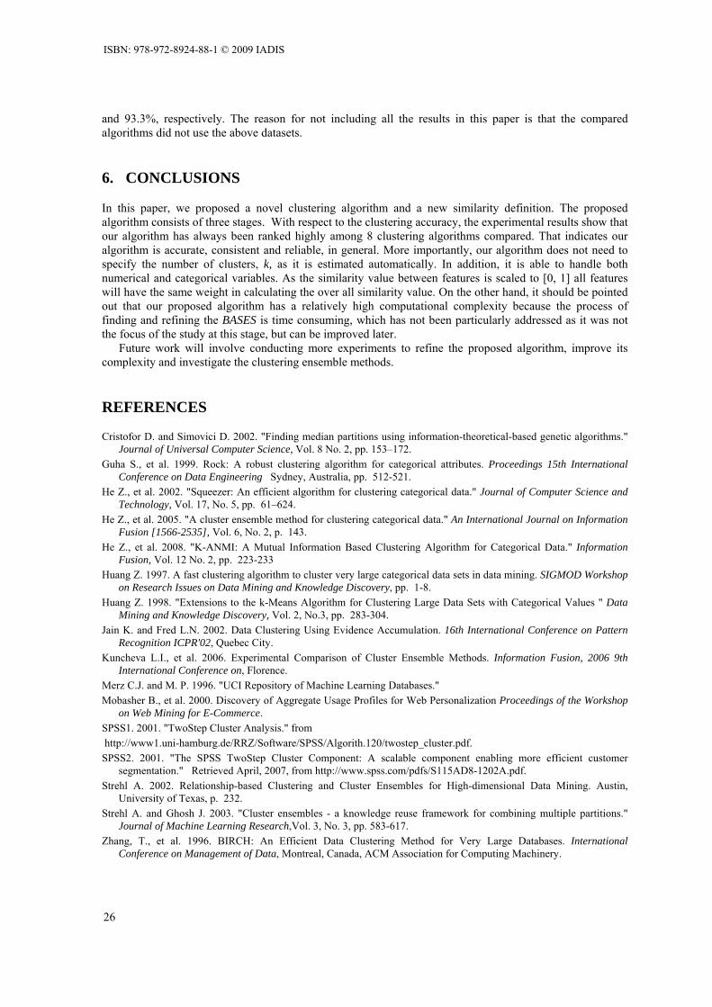
and 93.3%, respectively. The reason for not including all the results in this paper is that the compared algorithms did not use the above datasets.

6. CONCLUSIONS

In this paper, we proposed a novel clustering algorithm and a new similarity definition. The proposed algorithm consists of three stages. With respect to the clustering accuracy, the experimental results show that our algorithm has always been ranked highly among 8 clustering algorithms compared. That indicates our algorithm is accurate, consistent and reliable, in general. More importantly, our algorithm does not need to specify the number of clusters, k, as it is estimated automatically. In addition, it is able to handle both numerical and categorical variables. As the similarity value between features is scaled to [0, 1] all features will have the same weight in calculating the over all similarity value. On the other hand, it should be pointed out that our proposed algorithm has a relatively high computational complexity because the process of finding and refining the BASES is time consuming, which has not been particularly addressed as it was not the focus of the study at this stage, but can be improved later.

Future work will involve conducting more experiments to refine the proposed algorithm, improve its complexity and investigate the clustering ensemble methods.

REFERENCES

Cristofor D. and Simovici D. 2002. "Finding median partitions using information-theoretical-based genetic algorithms." Journal of Universal Computer Science, Vol. 8 No. 2, pp. 153–172.

Guha S., et al. 1999. Rock: A robust clustering algorithm for categorical attributes. Proceedings 15th International Conference on Data Engineering Sydney, Australia, pp. 512-521.

He Z., et al. 2002. "Squeezer: An efficient algorithm for clustering categorical data." Journal of Computer Science and Technology, Vol. 17, No. 5, pp. 61–624.

He Z., et al. 2005. "A cluster ensemble method for clustering categorical data." An International Journal on Information Fusion [1566-2535], Vol. 6, No. 2, p. 143.

He Z., et al. 2008. "K-ANMI: A Mutual Information Based Clustering Algorithm for Categorical Data." Information Fusion, Vol. 12 No. 2, pp. 223-233

Huang Z. 1997. A fast clustering algorithm to cluster very large categorical data sets in data mining. SIGMOD Workshop on Research Issues on Data Mining and Knowledge Discovery, pp. 1-8.

Huang Z. 1998. "Extensions to the k-Means Algorithm for Clustering Large Data Sets with Categorical Values " Data Mining and Knowledge Discovery, Vol. 2, No.3, pp. 283-304.

Jain K. and Fred L.N. 2002. Data Clustering Using Evidence Accumulation. 16th International Conference on Pattern Recognition ICPR'02, Quebec City.

Kuncheva L.I., et al. 2006. Experimental Comparison of Cluster Ensemble Methods. Information Fusion, 2006 9th International Conference on, Florence.

Merz C.J. and M. P. 1996. "UCI Repository of Machine Learning Databases." Mobasher B., et al. 2000. Discovery of Aggregate Usage Profiles for Web Personalization Proceedings of the Workshop

on Web Mining for E-Commerce. SPSS1. 2001. "TwoStep Cluster Analysis." from http://www1.uni-hamburg.de/RRZ/Software/SPSS/Algorith.120/twostep_cluster.pdf. SPSS2. 2001. "The SPSS TwoStep Cluster Component: A scalable component enabling more efficient customer

segmentation." Retrieved April, 2007, from http://www.spss.com/pdfs/S115AD8-1202A.pdf. Strehl A. 2002. Relationship-based Clustering and Cluster Ensembles for High-dimensional Data Mining. Austin,

University of Texas, p. 232. Strehl A. and Ghosh J. 2003. "Cluster ensembles - a knowledge reuse framework for combining multiple partitions."

Journal of Machine Learning Research,Vol. 3, No. 3, pp. 583-617. Zhang, T., et al. 1996. BIRCH: An Efficient Data Clustering Method for Very Large Databases. International

Conference on Management of Data, Montreal, Canada, ACM Association for Computing Machinery.

ISBN: 978-972-8924-88-1 © 2009 IADIS

26

BEHAVIOURAL FINANCE AS A MULTI-INSTANCELEARNING PROBLEM

Piotr JuszczakGeneral Practice Research Database, MHRA, 1 Nine Elms Lane,SW8 5NQ, London, United Kingdom

ABSTRACTIn various application domains, including image recognition, text recognition or the subject of this paper, be-havioural finance, it is natural to represent each example asa set of vectors. However, most traditional dataanalysis methods are based on relations between individualvectors only. To cope with sets of vectors, insteadof single vector descriptions, existing methods have to be modified. The main challenge is to derive meaningfulsimilarities or dissimilarities measures between sets of vectors. In this paper, we derive several dissimilaritiesmeasures between sets of vectors. The derived dissimilarities are used as rudiments of data analysis methods,such as kernel-based clustering and SVM classification. Theperformance of the proposed methods is examinedon consumer credit cards behaviour problems. These problems are shown to be an example of a multi-instancelearning problems.

KEYWORDSbehavioural finance, multi-instance learning

1. INTRODUCTION

Multiple Instance Learning (MIL) is a variation of supervised learning with labelled sets of vectors rather thanindividual vectors. In supervised learning, every training example is assigned with a discrete or real-valuedlabel. In comparison, in MIL the labels are only assigned to sets (also called bags) of examples. In the binarycase, a set is labelled positive if all examples in that set are positive, and the set is labelled negative if all theexamples in it are negative. The goal of MIL is, for example, to classify unseen sets based on the labelled setsas the training data.

For example, a gray value image can be considered as a collection of pixels, vectors of intensity values. Itis natural to compute the distance between such representedimages as a distance between sets of vectors. Thisapproach has a major advantage over the approach where features are derived from images, e.g. Gabor filters.Namely, if a meaningful distance is derived, the classes maybecome separable as information about examplesis not reduced to features.

Early studies on MIL were motivated by the problem of predicting drug molecule activity level. Subse-quently, many MIL methods have been proposed, such as learning axis-parallel concepts (Dietterich et al.,1997), diverse density (Maron & Lozano-Perez, 1998), extended Citation kNN (Wang & Zucker, 2000), tomention a few. These methods have been applied to a wide spectrum of applications ranging from imageconcept learning and text categorisation to stock market prediction.

The early MIL work (Dietterich et al., 1997) was motivated bythe problem of determining whether adrug molecule will bind strongly to a target protein. As the examples, some molecules that bind well (positiveexamples) and some molecules that do not bind well (negativeexamples) are provided. A molecule may adopta wide range of shapes or confrontations. Therefore, it is very natural to model each molecule as a set, withthe shapes it can adopt as the instances in that set. (Dietterich et al., 1997) showed that MIL approachessignificantly outperform normal supervised learning approaches which ignore the multi-instance nature of MILproblems.

(Maron & Lozano-Perez, 1998) partitioned natural scene pictures from the Corel Image Gallery into fixed


27

sized sub-images and applied a multi-instance learning algorithm, called diverse density (DD) to classify theminto semantic classes. (Yang & Lozano-Perez, 2000) used a similar approach for content-based image retrieval.(Zhang & Goldman, 2001) compared DD with an expectation-maximisation (EM) version of the DD algorithmfor image retrieval.

Similar to the argument made about images, a text document can consist of multiple passages concernedwith different topics, and thus descriptions at the document level might be too rough. (Andrews et al., 2002)applied SVM-based MIL methods to the problem of text categorisation, where each document is representedby overlapping passages.

The populark-Nearest Neighbour (k-NN) approach can be adapted for MIL problems if the distance be-tween sets is defined. In (Wang & Zucker, 2000), the minimum Hausdorff distance was used as the set-leveldistance metric, defined as the shortest distance between any two instances from each set. Using this set-leveldistance, we can predict the label of an unlabelled set. (Wang & Zucker, 2000) proposed a modifiedk-NNalgorithm called Citationk-NN.

In this paper, we follow a similar approach. We focus on derivation of distances between sets of vectorsand then use derived distances as a basis to define kernels or use them directly with distance-based analysismethods. The proposed distances are evaluated on behavioural finance problems.

2. DISTANCES BETWEEN SETS OF VECTORS

To show the challenge of distance derivation for MIL, consider the following example shown in figure 1. Thefirst subfigure, figure 1(a), shows a toy problem: a cup on a table with the table located on a floor. We wouldlike to define a distance between these three objects: cup (C), table (T) and floor (F). We are not necessarilyrestricted to an Euclidean distance, but chose an other possibility.

0 0.5 1 1.50

0.5

1

1.5

(a)

T F C

T 0 0 1

F 0 0 1

C 0 1 0

(b)

−1 −0.5 0 0.5 1−1

−0.5

0

0.5

1

T?CF

(c)

−1 −0.5 0 0.5 1−1

−0.5

0

0.5

1

positive distance

nega

tive

dist

ance

Pseudo−Euclidean space

T

CF

(d)

Figure 1. (a) Illustration Of A Toy Problem: A Cup (C), A Table(T) And A Floor (F), (b) Distances BetweenThe Three Objects, (c) Embedding Of Distances In An Euclidean Space, (d) Embedding Of Distances In APseudo-Euclidean Space.

As Euclidean distance is defined between points, the three objects have to be reduced to points, e.g. totheir centres of mass or centres of gravity. Therefore, the distance is not defined between objects but simplifiedversions of them. Alternatively we may define a distance between these objects as the smallest distance betweenany of their parts. Thus, since the cup touches the table, thedistance between them is zero. Since the tabletouches the floor, the distance between them is also zero. However, because the cup does not touch the floorthe distance between cup and floor is different from zero. Forexample, it may be set to one. Figure 1(b) showsa table with such computed distances between these three objects. Note however, that we can not embed thesedistances into a Euclidean space; see figure 1(c). To embed these relations one needs a much richer spacecalled Pseudo-Euclidean space (Pekalska & Duin, 2005). Thespace is constructed from a negative and positivepart; see figure 1(d). Dashed lines indicate zero distances between objects and continuous lines a boundary ofallowed distances. For a broader discussion on possible distance measures see (Pekalska & Duin, 2005).

This simple example shows the importance of the definition ofdistance. The example also shows somepitfalls that arise when objects are not represented as points. As a concrete example, in modern mathematicalphysics, string theoreticians face the problem of defining distance relations between strings and not simplypoints as in classical physics. This gives raise to new methods and new mathematics. In data analysis w oftenfind similar problems and would benefit from not reducing objects to points in a feature space.

ISBN: 978-972-8924-88-1 © 2009 IADIS

28

2.1 Proposed Distance Measures

In this paper we investigate the case when examples are presented as collectionsS = {x1,x2, . . . ,xn} of ddimensional vectorsxi ∈ Rd or xi ∈ S ⊂ R

d. Examples are associated with sets and labels are assigned tosets.

We denote positive sets asS+i , and thejth example in that set asS+

ij . Suppose each example can berepresented by a vector, and we useS+

ijk to denote the value of thekth feature of example. Likewise,S−

i

denotes a negative set andS−

ij thejth example in that set.Let us describe each setSi by a descriptor that enclose all vectors from that set. For example, we can

describe each set by the minimum volume sphere or ellipsoid that encloses all vectors from the set (Juszczak,2006; Juszczak et al., 2009). The similarity between two sets can be measured by the volume of a commonpart of these sets. Figure 2 shows two examples of descriptors with data vectors omitted for clarity.

2.1.1 Distance Based On Volume Of Overlapping Spheres

The simplest type of such a descriptor is a minimum volume sphere. As the first distance measure betweentwo sets,S1 andS2, we propose to measure distance based on the volume of the overlap between spheres. Wedescribe each set by a sphere of the minimum volume, that contain all the vectors from that set (Tax & Duin,2004). The volume of the overlapVo is a measure of the similarity between two sets, this volume is scale bydividing by the sum of volumes of spheres:

D(S1,S2) = 1 −Vo

VS(A1,R1) + VS(A2,R2)(1)

whereS(Ai, Ri) denote a sphere with a centreAi and radiusRi.

A1

A2

R1

R2rchc1hc2

(a)

Vo

(b)

Figure 2. Examples Of Similarity Measures Between Sets. Vectors Are Omitted For Clarity. (a) A SimilarityMeasure Based On An Overlap Between Two SpheresS(A1, R1) And S(A2, R2). (b) A Similarity MeasureBased On An Overlap Between Two An Arbitrary Shaped Descriptors.

The volume of a single overlapVo between two spheres equals the sum of volumes of two spherical caps.The spherical cap (Harris & Stocker, 1998) is a part of a sphere defined by its heighthc ∈ [0, 2R] and radiusrc ∈ [0, 2R]; see figure 2(a) where the overlap, the gray region in the figure, is created from two spherical capsbetween spheresS(A1, R1) andS(A2, R2).

Note that these two spherical caps have the same radiusrc but different heightshc. We have derived (seeAppendix for a derivation) the volume of ad-dimensional spherical cap as an integral ofd−1-dimensionalspheres over the heighthc of the cap:

Vcap(R, hc) =π(d−1)/2Rd−1

Γ((d − 1)/2 + 1)

βmax∫

0

sind−1(β)dβ

where

βmax = arcsin(√

(2R − hc)(hc/R2))

(2)


29

Therefore, the volume of a single overlapVo between two spheres can be computed as the sum of two sphericalcaps:

Vo = Vcap(R1, hc1) + Vcap(R2, hc2

) (3)

therefore the distanceD(S1,S2) between two setsS1 andS2 can be computed as:

D(S1,S2) = 1 −Vcap(R1, hc1

) + Vcap(R2, hc2)

VS(A1,R1) + VS(A2,R2)(4)

2.1.2 Related Work

There are several well-known definitions of similarity or distance between distributions, including the Kullback-Leibler divergence, Fisher kernel,χ2 distance (Duda et al., 2001).

As an example we will describe in more depths a similarity measure based on Bhattacharyya’s distancebetween distributions (Bhattacharyya, 1943),

K(x,x′) = K(p, p′) =

∫

√

p(x)√

p′(x)dx, (5)

For multivariate normal distributionsN (µ, Σ) Bhattacharyya’s distance can be computed in a close form (Dudaet al., 2001) as:

K(p, p′) = |Σ|−1

4 |Σ′|−1

4 |1

2Σ−1 +

1

2Σ

′−1|−

1

2 exp(−1

4µT Σ−1µ −

1

4µ

′T Σ′−1µ′

+1

4(Σ−1µ + Σ

′−1µ′)T (Σ−1 + Σ

′−1)(Σ−1µ + Σ

′−1µ′))

(6)

This similarity measure is proportional to a common part between two Gaussians that describe data.

3. BEHAVIOURAL FINANCE AS A MULTI-INSTANCE LEARN-ING PROBLEM

MIL has been used in several applications including image classification, document categorisation and textclassification. In this section we will show that problems inbehavioural finance can also be approached usingMIL techniques.

Financial institutions would like to classify customers not only based on static data, e.g. age, income,address, but also based on financial activities. These financial activities can be a set of transactions, loans,or investments on the market. In this paper we investigate financial behaviour based on transactions madein personal banking. In particular, we would like to find different patterns of behaviour for legitimate andfraudulent users in personal banking. The behaviour of an account owner is a set of transactions rather than asingle vector. Therefore, in this problem MIL methods can beapplied.

We would like to find whether legitimate or fraudulent patterns are clustered, and if so, determine if theclusters are consistent with the following statements:

1. Because fraudulent users have a single purpose in withdrawing money from an account their transactionsshould exhibit some patterns.

2. The constrains of daily life, the infrastructure and availability of card transaction facilities means we canexpect certain patterns of legitimate behaviour. For example, each of us have particular way of live, wework at certain hours, therefore can not use bank cards at this time, we earn certain amount of money,therefore our spending are limited, we withdraw money fromATMs that are close by work, home.

However, the singular objective of fraudulent use suggestswe should expect characteristically differentbehaviour.

ISBN: 978-972-8924-88-1 © 2009 IADIS

30

We explore corrections of these two statements with two realworld data sets and present an empiricalanalysis of the behavioural patters.

Each activity record, a transaction on a bank account is described by several features provided by ourcommercial collaborators. From this set we select a subset of features which are relevant to behavioural finance.We describe activities on accounts by answering questions like: when?, where?, what?, how often? Specifically,the features we use to describe a transaction are:

amount mi, the amount in pence of a transaction,

amount difference mi−1 − mi, difference in amount between current and last transaction(the differencebetween first and second transaction is also calculated for the first transaction and for any other featurethat applied),

amount sum mi−1 + mi, sum of the amount of the current and previous transaction,

amount product mi−1 × mi, product of the amount of the current and previous transaction,

time ti transaction time, in seconds after midnight,

transaction interval ti − ti−1, time, in seconds, from the previous transaction,

service ID indicator for POS (Point of sale) or ATM (Automated teller machine) transaction,

Merchant type categorical indicator indicating merchant type,

ATM-ID categorical identifier for each ATM.

Looking at individual accounts one can observe several types of behaviour. For example, examine the threeaccounts shown in figure 3. The figure shows three accounts (columns) described by three features (rows). Theestimated probability density function (pdf) is computed for each feature. We can see that the first accountowner (first column) withdraws money in the mornings, in small amounts, and in the period of 24 hours.The second account owner makes transactions during the entire day, withdrawing a little more money but lessfrequently. The third account owner transacts mostly in theevenings, withdrawing the greatest amount ofmoney with periodic intervals.

Financial institutions group their customers based on a setof rules and put them to associate clusters. Wewould like to verify whether instead there are ”natural”, supported by real data, groups of behaviour in plasticcard transaction data, and assess their number and nature.

4. EXPERIMENTS

Our commercial collaborators have provided a number of plastic card transaction data sets observed over shortperiods since2005. We use two of these data sets,D1 andD2, with characteristics described in Table 1. Afraudulent account inD1 has15 fraud transactions on average. The average forD2 is different, reflecting theslightly different nature of the contributing organisations. For reasons of commercial confidentiality we cannotdivulge more information about the data. Note that both datasets are large and richly structured, and significantpre-processing was required to extract suitable data for analysis.

In the following experiments, we omit accounts for which fraud occurred within the first10 transactions, asmodels need some minimal information for training. We used accounts with at least50 legitimate transactionsand with at least5 fraudulent transactions.

Table 1. Characteristics Of Data Sets.

#of accounts #transactions #fraud accounts #fraud transactions period (months)D1 44637 2374311 3742 58844 3D2 11383 646729 3217 18501 6


31

account 1 account 2 account 3

0 2 4 6 8

x 104

0

0.002

0.004

0.006

0.008

0.01

12am

30 trans.

pdf

time of day [s]0 2 4 6 8

x 104

0

0.5

1

1.5

2

2.5

3

x 10−3

12am

63 trans.

pdf

time of day [s]0 2 4 6 8

x 104

0

0.5

1

1.5

2

2.5

3

3.5

4

x 10−3

12am

53 trans.

pdf

time of day [s]

0 2 4 6 8 10

x 104

0

0.005

0.01

0.015

0.02

30 trans.

pdf

money [p]0 0.5 1 1.5 2

x 104

0

0.005

0.01

0.015

0.02

0.025

0.03

63 trans.pdf

money [p]0 0.5 1 1.5 2

x 104

0

0.005

0.01

0.015

0.02

0.025

0.03

53 trans.

pdf

money [p]

0 2 4 6 8 10 12

x 105

0

0.5

1

1.5

2

2.5

3

3.5

4x 10

−3

30 trans.

pdf

time [s]0 2 4 6 8 10 12

x 105

0

1

2

3

4

5

6x 10

−3

63 trans.

pdf

time [s]0 2 4 6 8 10 12

x 105

0

0.002

0.004

0.006

0.008

0.01

0.012

0.014

53 trans.

pdf

time [s]

Figure 3. Probability Density Functions(PDF) Estimated On Legitimate Transactions, From Three Accounts(Columns), Described By Three Features (Rows). The First Row Shows The Time Of Day, In Seconds, WhenTransactions Are Made. The Second Row Shows The Amount Of Money, In Pennies, That Has Been With-drawn And The Third Row Time Periods Between Transactions, In Seconds.

4.1 Clustering Of Fraudulent And Legitimate Behaviours

To verify if fraudulent or legitimate patterns are clustered we compute a distance based on equation (4) between2000 randomly selected legitimate and2000 fraudulent accounts fromD1 andD2. Sorted distance matricesare shown in the first row of figure 4. The matrices were sorted using the VAT algorithm (Bezdek & Hathaway,2002).

To cluster patterns we use a kernel based clustering proposed in (Girolami, 2001) with a Gaussian kerneland complexity parameters optimised by maximum likelihood. The dendrograms are shown in the bottom rowof figure 4.

From figure 4 we can see that fraudulent behaviours are more clustered than legitimate behaviours, howeverin both groups there are visible clusters, corresponding topatterns of behaviours. Since fraudsters have a singlepurpose in withdrawing money they tend to be more clustered than legitimate patterns. These conclusionsagree with our expectations, however now it is also supported by real data. Now a new set of transactions canbe assessed as being similar to a set of transaction that is already in a dataset.

5. CONCLUSIONS

We have proposed a distance measure between sets of vectors based on the volume of overlap between thesmallest enclosing spheres. It has been shown that problemsin behavioural finance can be approached by multi-instance methods. Based on the proposed distance measure weinvestigate ”natural” groups in legitimate andfraudulent personal banking behaviour. It has been shown that as fraudsters has a single purpose in withdrawingmoney they behavioural patterns tend to be more clustered than those of legitimate users.

ISBN: 978-972-8924-88-1 © 2009 IADIS

32

0.5

0.6

0.7

0.8

0.9

1

(a) fraudD1

0.5

0.6

0.7

0.8

0.9

1

(b) fraudD2

0.5

0.52

0.54

(c) legitimateD1

0.5

0.55

0.6

(d) legitimateD2

Figure 4. Distance Matrices And Dendrograms For FraudulentAnd Legitimate Patterns In Data SetsD1 AndD2.

6. ACKNOWLEDGEMENTS

The views expressed in this paper are those of the authors anddo not reflect the official policy or position ofthe MHRA.

Appendix: The Volume Of A Spherical Cap

The spherical cap is part of a sphere as shown in figure 5. When two spheresS(A1, R1) andS(A2, R2)intersect, a heighthc and a radiusrc of the two cups can be derived simply from Pythagoras equations as:

hc1= R1 −

‖A1 − A2‖2 − R22 + R2

1

2‖A1 − A2‖, hc2

= R2 −‖A1 − A2‖2 + R2

2 − R21

2‖A1 − A2‖

rc1=

√

R21 − (R1 − hc1

)2 = rc2=

√

R22 − (R2 − hc2

)2

The volume of a single cap can be computed by integrating the volumes ofd−1 dimensional spheres from theradiusrc to 0 over different value of a heighthc.

R

hc

R − hc

βmax

rc

Figure 5. Spherical Cap.

Vcap =2π(d−1)/2

Γ((d − 1)/2 + 1)

hc∫

0

rN−1c (hc)dhc (7)

From figure 5 it can be seen that:

r2c + (R − hc)

2 = R2, (8)

rc = R sin(βmax). (9)

Substituting those equations gives:

Vcap =2π(d−1)/2Rd−1

Γ((d − 1)/2 + 1)

βmax∫

0

sind−1(β)dβ (10)


33

βmax = arcsin(√

(2R − hc)(hc/R2)) (11)

The integral∫

sind−1(β)dβ can be handled by recursion (Bronshtein et al., 1997,§ 8).

∫

sind−1(β)dβ = −sind−2 β cosβ

d − 1+

d − 2

d

∫

sind−3 βdβ (12)

7. REFERENCES

Andrews, S., Tsochantaridis, I., & Hofmann, T. (2002). Support vector machines for multiple-instance learning.Neural Information Processing Systems(pp. 561–568).

Bezdek, J. C., & Hathaway, R. J. (2002). VAT: a tool for visualassessment of (cluster) tendency.Proceedingsof the International Joint Conference of Neural Networks(pp. 2225–2230). IEEE Press, Piscataway, NJ.

Bhattacharyya, A. (1943). On a measure of divergence between two statistical populations defined by theirprobability distributions.Bull. Calcutta Math Soc.

Bronshtein, I. N., Semendyayev, K. A., & Hirsch, K. A. (1997). Handbook of mathematics. Springer-VerlagTelos.

Dietterich, T., Lathrop, R. H., & Lozano-Perez, T. (1997).Solving the multiple instance problem with axis-parallel rectangles.Artificial Intelligence, 89, 31–71.

Duda, R. O., Hart, P. E., & Stork, D. G. (2001).Pattern classification. John Wiley & Sons. second edition.

Girolami, M. (2001). Mercer kernel based clustering in feature space.I.E.E.E. Transactions on Neural Net-works.

Harris, J. W., & Stocker, H. (1998).Handbook of mathematics and computational science. New York: Springer-Verlag.

Juszczak, P. (2006).Learning to recognise. A study on one-class classification and active learning.Doctoraldissertation, Delft University of Technology. ISBN: 978-90-9020684-4.

Juszczak, P., Tax, D. M. J., Pekalska, E., & Duin, R. (2009). Minumum volume enclosing ellipsoid datadescription.Journal of Machine Learning Research, under revision.

Maron, O., & Lozano-Perez, T. (1998). A framework for multiple-instance learning.Neural InformationProcessing Systems(pp. 570–576). The MIT Press.

Pekalska, E., & Duin, R. P. W. (2005).The dissimilarity representation for pattern recognition: foundationsand applications. River Edge, NJ, USA: World Scientific Publishing Co., Inc.

Tax, D. M. J., & Duin, R. P. W. (2004). Support vector data description. Machine Learning, 54, 45–56.

Wang, J., & Zucker, J. (2000). Solving the multiple-instance problem: A lazy learning approach.Proc. 17thInternational Conf. on Machine Learning(pp. 1119–1125). Morgan Kaufmann, San Francisco, CA.

Yang, C., & Lozano-Perez, T. (2000). Image database retrieval with multiple-instance learning techniques.Proc. of the 16th Int. Conf. on Data Engineering(pp. 233–243).

Zhang, Q., & Goldman, S. A. (2001). EM-DD: An improved multiple-instance learning technique.NeuralInformation Processing Systems(pp. 1073–1080). MIT Press.

ISBN: 978-972-8924-88-1 © 2009 IADIS

34

BATCH QUERY SELECTION IN ACTIVE LEARNING

Piotr JuszczakGeneral Practice Research Database, MHRA, 1 Nine Elms Lane,SW8 5NQ, London, United Kingdom

ABSTRACTIn the active learning framework it is assumed that initially a small training setXt and a large unlabelled setXu are given. The goal is to select the most informative object from Xu. The most informative object is theone, that after revealing its true label by the expert, and adding it to the training set improves the knowledgeabout the underlying problem the most, e.g. improves the most the performance of a classifier in a classifica-tion problem. In some practical problems however, it is necessary to select at the same time more than a singleunlabelled object to be labelled by the expert. In this paper, we study pitfalls and merits of such selection. Weintroduce active learning functions that are especially useful in the multiple query selection. The performanceof the proposed algorithms are compared with standard single query selection algorithms on toy problems andtheUCI repository data sets.

KEYWORDSactive-learning, multiple query selection

1. INTRODUCTION

In the traditional approach to statistical learning, one tries to determine a functional dependency between somedata inputs and their corresponding outputs, e.g. their class labels. This is usually estimated based on a given,fixed set of labelled examples. Active sampling (Lewis & Gale, 1994; Cohn et al., 1995; Roy & McCallum,2001; Juszczak & Duin, 2004) is an alternative approach to automatic learning: given a pool of unlabelled dataXu, one tries to select a set of training examples in an active way to reach a specified classification error witha minimum cardinality. Therefore, ideally the same classification error is achieved with a significantly smallertraining set. The criterion of how informative a new object is depends on what we are interested in. We mayselect a new object to be maximally informative about parameter values of a classifier or select objects only fromsome regions, e.g. around a region that we are not able to sample directly, to improve classification accuracyonly locally. Finally to select objects to minimise a probability of training models with large errors (Juszczak,2006).Definition 1. We can define an active learning function as a functionF that assigns a real value to eachunlabelled objectF(xi) → R, xi ∈ Xu. Based on this criterion we can rank unlabelled objects and select themost informative object,x∗, according toF :

x∗ ≡ arg max

xi∈Xu

F(xi) (1)

In this paper, the most informative object,x∗ ∈ Xu, is defined as the one, that after revealing its label and

adding to the training set improves performance of a classifier the most. In this paper, we focus on pool-based active learning (Lewis & Gale, 1994; Cohn et al., 1995;Roy & McCallum, 2001; Juszczak & Duin,2004). In this learning scheme there is an access to a small set of labelled objectsXt, a training set, and alarge pool of unlabelled objectsXu. Objects are usually selected one by one according to a specified activelearning functionF . Active learning is usually compared to passive learning, in which unlabelled objects aresampled randomly, i.e. according to the probability density functionP (X). The performance is measured asa generalisation error obtained on an independent test set.The general framework of pool-based active learningis presented in Algorithm 1 and learning curves for the two sampling are shown in figure 1.


35

Algorithm 1 A General Framework Of Pool-based Active Learning.Assume that an initial labelled training setXt, a classifierh, a active functionF and unlabelled dataXu aregiven.

1. Train classifierh on the current training setXt; h(Xt).

2. Select an objectx∗ from the unlabelled dataXu according to the active query functionx∗ ≡ arg maxxi∈Xu

F(xi).

3. Ask an expert for the label ofx∗. Enlarge the training setXt and reduceXu.

4. Repeat steps (2)–(4) until a stopping criterion is satisfied, e.g. the maximum size ofXt is reached.

In some practical problems however, there is a need to selectmultiple queries to be labelled by the expertat the same time. Such problems are usually problems where expert knowledge is required not constantly butin time intervals, e.g. financial markets, medical intensive care units or remote control of machines. Let us take

as an example a medical intensive care device where conditionlabels (normal/abnormal) that a doctor assigns changes in time.Therefore, the classifier needs to be update in time as a conditionof a patient improves or deteriorates changing meaning of mea-surements. It is much more practical, if the doctor adjusts theclassifier by assigning labels to several preselected measurementseach hour or day, than assigning constantly a label to a single se-lected measurement; e.g. per minute or even a second. The sameholds for sensors in automated factories or predictors in stock mar-ket. Measurement labels may need adjustments as they definitionschange in time. Similarly to the active learning approach, whereone draws a single unlabelled object, here the goal is to learn aninput-output mappingX → ω from a set ofn training examplesXt = {xi, ωi}

ni=1, wherexi ∈ X , ω(j)

i ∈ [ω(1), . . . , ω(C)] and thesizen of the training set should be minimised.

0 50 100 150 200

0.05

0.1

0.15

0.2

0.25

number of queries

mea

n er

ror

active samplingrandom sampling

cost reduction

error reduction

Figure 1. Expected Learning CurvesFor Active And Random Sampling.

However now, at each iteration, the active learner is allowed to select a multiple, new training input{x1, . . . ,xk}∗ ∈ Xu of k elements from the unlabelled dataXu. Note thatk can be much larger than1.The selection of{x1, . . . ,xk}∗ may be viewed as a query based on the following active sampling function:

{x1, . . . ,xk}∗ ≡ arg max

{x1,...,xk}∗∈Xu

k∑

i=1

F(xi|h(Xt), Xt) (2)

Having selected{x1, . . . ,xk}∗, the learner is provided with the corresponding labels[ω1, . . . , ωk] by an expert,as a result of an experiment or by some other action. The new training input{x∗

j , ωj}kj=1 is added to the

current training setXt = Xt ∪ {x∗

j , ωj}kj=1 and removed from the unlabelled setXu = Xu\{x1, . . . ,xk}∗.

The classifier is retrained and the learner selects another set {x1, . . . ,xk}∗. The process is repeated until theresources are exhausted, the training set reached a maximumnumber of examples, or the error reaches anacceptable level.

Since in the standard active sampling algorithms, the classifier is recomputed after each query, the valuesof an active sampling functionF , based on such a classifier, change as well. Therefore, unlabelled objects,that are queried, differ in consecutive draws. However, if we consider the simultaneous selection of multipleobjects,k > 1, similar objects are selected in a single draw. To illustrate this in figure 2(a) five objects withthe highest values of two active learning functions,F1 andF2 are shown. Here we used Probability DensityCorrection (pdc) andMinMax (Juszczak, 2006). It can be observed that for each sampling method the selectedobjects are chosen from the same region in the feature space.These active learning methods do not considerthe fact of revealing a label of a single query on the remaining queries. Therefore, adding such a batch is notsignificantly more beneficial than adding just its single representative. For clarity of a figure we only showthese two methods, however the same problem holds for all active learning methods that select a single query.

ISBN: 978-972-8924-88-1 © 2009 IADIS

36

When we would like to select multiple queries in active sampling we should consider not only the criterionthey are based on, e.g. the uncertainty of labels of unlabelled objects, but also the effect of obtaining a classlabel of a single candidate object on the remaining candidate objects. In this paper we investigate this problem.

−8 −6 −4 −2 0 2 4 6 8

−8

−6

−4

−2

0

2

4

6

(a)

Xt,ω=1

Xt,ω=2

Xu

F1

F2

−8 −6 −4 −2 0 2 4 6 8

−8

−6

−4

−2

0

2

4

6

(b)

Figure 2. (a) Five Objects Selected ByF1 AndF2 Active Learning Functions. The Classifier,1-NN (1-NearestNeighbour), Is Drawn As Solid Line. (b) Five Objects Selected ByF1 AndF2 Considering Also The InfluenceOf Reviling Labels Of Other Objects In The Batch.

2. QUADRATIC PROGRAMMING QUERY DIVERSIFICATIONWe formulate three active query selection algorithms suitable for the selection of informative batches of unla-belled data. The diversification criterion in these algorithms is related to the type of a classifier, e.g. distanceor density based, that is going to be trained on the selected objects. Such ’personalisation’ of queries is helpfulin human learning. Different people may require different examples to learn efficiently certain concepts. Thesame also holds for classifiers. For some classifiers selecting unlabelled objects; e.g. with a maximum un-certainty change their decision boundary locally, e.g. forthe1-NN (1-Nearest Neighbour) rule. Selecting thesame object for a parametric classifier, e.g. the mixture of Gaussians classifier changes the decision boundaryglobally. This also holds for kernel based methods such asSVM. Therefore, a good sampling function shouldalso include, in its estimation of potential queries, properties of the classifier itself.

In particular, we propose three active sampling methods with diversification criteria based on distances,densities and inner products between labelled and unlabelled objects. The presented three active samplingmethods are generic and can be used with any type of a classifier, however, because they compute the utilitycriteria in a certain way they are especially useful for classifiers that are based on the same principles e.g. the1-NN rule, the Parzen classifier andSVM.

2.1 Distance-based DiversificationAs was mentioned in the introduction the most informative batch of unlabelled objects should contain objectsthat have the minimum influence on the classification labels of each other. Intuitively, this can be relatedto distances between objects in a batch i.e. by maximising the sum of distances

∑ki

∑kj D(xi,xj) between

objects to be selected. For small distances between objectswe expect redundant class information. If we givea weight0 ≤ αi ≤ 1 to each objectxi ∈ Xu, the above sum can be written asmaxα α

T Dα, αT1 = k for

a sparse solution. Additionally, we are interested in the objects that have information about labels of other notyet selected unlabelled objects, e.g centres of clusters inXu can be expected to describe remaining unlabelleddata in their clusters. To impose this, we can simply demand that the distanceDnn(xi) = ‖µnn(xi) − xi‖between objectxi and the meanµnn(xi) of its nearest neighbours should be minimum; see figure 3. Note thatµnn(xi) is computed on the set of nearest neighbours ofxi but withoutxi. SinceDnn(xi) describes only asingle object this linear term can be subtracted from the previous quadratic term asmaxα α

T Dα − αDnn,α

T1 = k. An active learning functionF(x) should have a high value for the selected objects. This is also

a linear term, therefore the selection of objects with the highest values for these three criteria can be writtenasmaxα α

T Dα + αT (F − Dnn), α

T1 = k. We compute the utility of the batch ofk unlabelled objects

by maximising the above formula using a quadratic programming technique. This allows us to optimise theentire batch at once compared to iterative procedures whichexamine a single object in the batch at a time, asdescribed in the next section. The diversification of queries, for a particular active learning functionF , basedon distances as a diversification criteria is written as:


37

maxα

αTDα + α

Tρ,

s.t. αT1 = k; 0 ≤ αi ≤ 1,

ρ = F − Dnn.

(3)

Dnn(xi)

xi

µnn(xi)

Figure 3. The Distance Between An Ob-jectxi And The Mean Of Its Nearest Neigh-bours.

The Euclidean distance matrixD, is not, in general, positive definite(zT Dz � 0, ∀z ∈ RN ). The positive def-

initeness, or the negative definiteness, of the matrixD is required by Kuhn-Tucker conditions (Rustagi, 1994)for the quadratic optimisation to converge to the global minimum or maximum. However, several techniquescan be used to transform a symmetric matrix to the positive (negative) definite one. For example one can applyclipping D = QpΛ

1/2p , whereΛp are only the positive eigenvalues, or simply taking the square Hadamard

powerD∗2 (D∗2 = d2ij) and adding a small constant to the diagonalD = diag(D∗2) + c (Gower, 1986).

In the optimisation (3), we are looking fork unlabelled objectsx for which the optimised functionαTDα+α

T ρ is maximum. Such a criterion can be used in general with any type of classifier but is especially suited forthe Nearest-Neighbour classifier, since it is based on distance relations between objects.

2.2 Density-based DiversificationFor density-based classifiers the diversification criterion can include a vector of densitiesP (x) instead ofdistancesDnn as such classifiers are based on densities. We can consider densities of unlabelled objects orthe relative difference between densities of labelled and unlabelled objects∆P (xi) = P (xi|Xu) − P (xi|Xt),wherex ∈ Xu; see figure 4. The quadratic programming optimisation lookssimilar to the above optimisationfor the Nearest-Neighbour classifier, except now the linearterm depends on the difference in density estimates.

maxα

αTDα + α

Tρ

s.t. αT1 = k, 0 ≤ αi ≤ 1,

ρ = F + ∆P.

(4) P (x|Xu) − P (x|Xt)

Figure 4. The Positive Difference∆P In Density Estimates ForLabelledXt : {+, •} And UnlabelledXu : {◦} Objects PlottedAs Isolines, The Current Classifier Boundary,Parzen Is DrownAs A Solid, Thick Line.

Such a method selects a batch of unlabelled objects with large distancesD between selected objects and withthe large density value in places where we have no samples yet. Finally the value of the active learning functionF should be also significantly large. In figure 4 we can easily point to five unlabelled objects with high valueof ∆P indicated by the centres of the concentric isolines. Such objects are remote from each other and arecentres of clusters. These make them a potentially informative batch to ask an expert for labels. Since thisdiversification method is based on a density estimation it isparticularly suitable for density based classifierse.g. theParzen, Quadratic (QDA) or Linear Discriminant Analysis (LDA).

ISBN: 978-972-8924-88-1 © 2009 IADIS

38

2.3 Boundary-based Diversification

The last type of a classifier we are considering is the SupportVector Machine (SVM). ForSVM it is convenient toexpress the mutual label relations of possible labels of unlabelled objects in terms of inner products or similarlythe angle between vectors. The angle between two vectorsxi andxj can be expressed as follows:

∠(xi,xj) = arccosx

Ti xj

‖xi‖‖xj‖= arccos

K(xi,xj)√

K(xi,xi)K(xj ,xj)(5)

wherexTi xj denotes the inner product andK is the between Gram matrix. Similarly to the optimisation (3) for

1-NN we would like to select objects for which the sum of their angles is maximum and additionally they arecentres of clusters in the Hilbert spaceH. For the Gaussian kernel the denominator in equation (5) becomes1. Since the Gramm matrixK is already positive definite it is easier to minimise the sum of inner productsbetween objects in the batch, instead of maximising the sum of square angles between selected objects:

minα

αT Kα − α

Tρ

s.t. αT1 = k, 0 ≤ αi ≤ 1,

ρ = F + Knn.

(6)

w0

x1

x2x3

sv1

sv2

sv3

sv4

sv5

Figure 5. Equal Division Of The Approximated VersionSpace By Three Unlabelled Objects{x1,x2,x3}. sv Indi-cates Five Support Vectors And Gray Circle Margin OfSVM.

whereKnn(xi) = ‖µnn(K(xi, :)) − K(xi, :)‖ is the difference between vectorK(xi, :) and the mean of itsneighbours inH.

Figure 5 presents a general idea of such a sampling. Let us assume that the problem is linearly separablein the feature space. This means that a version space (Mitchell, 1997) of a particular problem is non-empty. Inthe case ofSVM, we can approximate the version space by the support objectsand select objects that for twopossible labels divide equally such an approximated version space (Tong & Koller, 2000). Regardless of thetrue class labels we always reject that half of the classifiers that is inconsistent with the labels of the trainingdata. The tacit assumption is that classifiers are uniformlydistributed, i.e. each classifier from the version spaceis equally probable.

When we consider the selection of a batch of unlabelled objects an informative batch should contain objectsthat divide the version space equally. The selection of suchobjects implies that for all their possible labels thesize of the version space is maximally minimised; see figure 5. Unlabelled objects{x1,x2,x3} divide equallythe version space restricted by support vectors{sv1, . . . , sv5}.

3. RELATED WORKIn this section we shortly explain the difference between our query diversification algorithms and existingmethods. In particular, we relate our work to (Brinker, 2003; Park, 2004; Lindenbaum et al., 2004). Thesepapers present query diversification methods based on various criteria, e.g. similar to the proposed methods,distance between queries (Lindenbaum et al., 2004) or angles between queries in a batch (Brinker, 2003; Park,2004). In particular (Lindenbaum et al., 2004) proposed forthek-NN rule to construct a batch of unlabelleddata using an iterative procedure. At each step a single object is added to a batch that has a large value of anactive learning function and a large distance to already selected objects in a batch. Next, such a constructedbatch is presented as a query to an expert. (Brinker, 2003; Park, 2004) discusses similar iterative algorithmsfor theSVM. However, instead of selecting objects with the maximum sumof distances, they proposed to selectobjects based on the inner product relations. The algorithms select unlabelled objects that after including them


39

to the training set yield the most orthogonal hyperplanes.A simplified scheme of the existing algorithms is shown inAlgorithm 2. First, an algorithm selects a single unlabelledobject with the maximum value of a particular active learn-ing functionF . Then the next objects are added to a batchB for which either the sum ofF and distances to the objectsalready present in the batchD(x,B) is large (Lindenbaumet al., 2004) or the inner products are small (Brinker, 2003;Park, 2004). The process is repeated until the required cardi-nality ofB is reached.

Algorithm 2 Standard Diversification Algo-rithm.B = [ ]x∗ = arg maxx∈Xu

F(x)repeat

1. B = B ∪ {x∗}; Xu = Xu\{x∗}

2. x∗ = arg maxx∈Xu

[F(x) + D(x,B)]

until |B| = k

Because existing algorithms consider a single candidate tobe added to a batch and not an entire batch, they donot necessary select the most informative set of unlabelledobjects. The sum of distances and an active learningfunction do not necessarily reach their maxima for the selected batch. Moreover, the methods presented in thesepapers maximise distances, or minimise inner products, only between the selected objects; they do not take intoaccount the distribution of unlabelled data. Such methods are sensitive to the presence of outliers, by selectingobjects that are far from each other, and not, like in the proposed method, centres of local neighbourhood.

4. EXPERIMENTSAs an illustration, we first test the proposed query diversification algorithms on the artificialRubik’s cubedataset (Juszczak, 2006). It is a3 × 3 × 3 mode,3D, two-class data set with an equal number of objects per class.This data set, although not realistic to occur in practice, shows clearly the point of the query diversification foractive learning methods when multiple queries are to be selected.

In our experiments the initial labelled training setXt contains two randomly drawn objects per class. Thelearning proceeds with the queries ofk = {1, 8, 16, 32, 64} elements. First, in each iteration, a single objectis added to the current training set, a query of sizek = 1, then the learning process is repeated for the queryof sizek = 8, 16 and so on. The learning curve determined for the query based on a single object,k = 1, isused as the baseline. The goal is to achieve the performance which is at least as good as obtained for the singleobject selection algorithm.

Objects are selected according to the uncertainty sampling(Lewis & Gale, 1994)1. The learning curvesfor the1-NN rule, theParzen and theν-SVM with a radial-basis kernel are shown in figure 6. The error ismeasured on an independent test set. The results are averaged over100 random splits of all data into an initialtraining set, unlabelled data and a test set. The smoothing parameter of theParzen classifier is optimisedaccording to the maximum likelihood criterion (Duin, 1976)and theν for ν-SVM is set to the1-NN leave-one-out error on the training set. In the cases when this error is zero, theν is set toν = 0.01. σ in the radial-basiskernel is chosen as the averaged distance to the⌊

√

|Xt|⌋-nearest neighbour inXt.Gray learning curves represent sampling without query diversification and black learning curves present

sampling with query diversification. By observing gray curves it can be seen that by increasing the querysize, the number of objects necessary to reach the minimum error classifier increases. This phenomenon isunderstandable since data are highly clustered and selecting queries based on the active sampling criterion, e.g.the uncertainty sampling, leads to the selection of similarobjects from a single mode2.

The black learning curves in figure 6 show the results of the same experiments with the proposed querydiversification algorithms, for three types of classifiers for the same batch size. It can be seen that by diversify-ing queries using the proposed algorithms, the error drops,in this particular learning problem on average about5% and the difference in the number of queries that is necessary to reach the certain classification error is inaverage50 − 100 in all figures.

Next, we tested the proposed query diversification algorithm on data sets from the UCI repository (Hettichet al., 1998). Initial training sets consist of two objects per class. Because the experiments with all three

1The uncertainty sampling was chosen as an example, however the experimental results are similar for other selective sampling meth-ods (Juszczak, 2006).

2For a two-class problem with an equal number of objects per class, the average error in the beginning of the learning process is largerthan0.5. This is caused by the symmetric mode structure of the data set itself. Since every mode is surrounded by modes belonging to theother class additional labelled set causes, in the beginning, misclassification of objects from adjacent modes. By increasing the number ofclusters, this phenomenon lasts longer.

ISBN: 978-972-8924-88-1 © 2009 IADIS

40

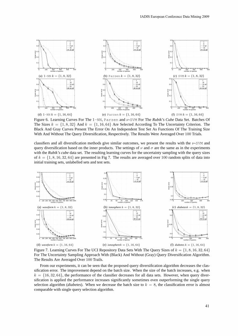
0 100 200 300 400 5000

0.1

0.2

0.3

0.4

0.5

number of queries

mea

n er

ror

188 qd3232 qd

(a) 1-NN k = {1, 8, 32}

0 100 200 300 400 5000

0.1

0.2

0.3

0.4

0.5

number of queries

mea

n er

ror

188 qd3232 qd

(b) Parzen k = {1, 8, 32}

0 100 200 300 400 5000

0.1

0.2

0.3

0.4

0.5

number of queries

mea

n er

ror

188 qd3232 qd

(c) SVM k = {1, 8, 32}

0 100 200 300 400 5000

0.1

0.2

0.3

0.4

0.5

number of queries

mea

n er

ror

11616 qd6464 qd

(d) 1-NN k = {1, 16, 64}

0 100 200 300 400 5000

0.1

0.2

0.3

0.4

0.5

number of queries

mea

n er

ror

11616 qd6464 qd

(e) Parzen k = {1, 16, 64}

0 100 200 300 400 5000

0.1

0.2

0.3

0.4

0.5

number of queries

mea

n er

ror

11616 qd6464 qd

(f) SVM k = {1, 16, 64}

Figure 6. Learning Curves For The1-NN, Parzen andν-SVM For TheRubik’s CubeData Set. Batches OfThe Sizesk = {1, 8, 32} And k = {1, 16, 64} Are Selected According To The Uncertainty Criterion. TheBlack And Gray Curves Present The Error On An Independent Test Set As Functions Of The Training SizeWith And Without The Query Diversification, Respectively. The Results Were Averaged Over100 Trials.

classifiers and all diversification methods give similar outcomes, we present the results with theν-SVM andquery diversification based on the inner products. The settings ofν andσ are the same as in the experimentswith theRubik’s cubedata set. The resulting learning curves for the uncertaintysampling with the query sizesof k = {1, 8, 16, 32, 64} are presented in Fig 7. The results are averaged over100 random splits of data intoinitial training sets, unlabelled sets and test sets.

0 100 200 300 400 500 600 700 800 900 1000

0.15

0.16

0.17

0.18

0.19

0.2

number of queries

mea

n er

ror

188 qd3232 qd

(a) waveformk = {1, 8, 32}

0 25 50 75 100 125 150 1750.05

0.1

0.15

0.2

0.25

0.3

number of queries

mea

n er

ror

188 qd3232 qd

(b) ionospherek = {1, 8, 32}

0 100 200 300 3830.28

0.3

0.35

0.4

0.43

number of queries

mea

n er

ror

188 qd3232 qd

(c) diabetesk = {1, 8, 32}

0 100 200 300 400 500 600 700 800 900 1000

0.15

0.16

0.17

0.18

0.19

0.2

number of queries

mea

n er

ror

11616 qd6464 qd

(d) waveformk = {1, 16, 64}

0 25 50 75 100 125 150 1750.05

0.1

0.15

0.2

0.25

0.3

number of queries

mea

n er

ror

11616 qd6464 qd

(e) ionospherek = {1, 16, 64}

0 100 200 300 3830.28

0.3

0.35

0.4

0.43

number of queries

mea

n er

ror

11616 qd6464 qd

(f) diabetesk = {1, 16, 64}

Figure 7. Learning Curves For The UCI Repository Data Sets With The Query Sizes ofk = {1, 8, 16, 32, 64}For The Uncertainty Sampling Approach With (Black) And Without (Gray) Query Diversification Algorithm.The Results Are Averaged Over100 Trails.

From our experiments, it can be seen that the proposed query diversification algorithm decreases the clas-sification error. The improvement depend on the batch size. When the size of the batch increases, e.g. whenk = {16, 32, 64}, the performance of the classifier decreases for all data sets. However, when query diver-sification is applied the performance increases significantly sometimes even outperforming the single queryselection algorithm (diabetes). When we decrease the batch size tok = 8, the classification error is almostcomparable with single query selection algorithm.


41

5. CONCLUSIONSWe have studied the problem of selecting multiple queries ina single draw based on a specified active learningfunction. In such a selection, a learner might yield a systematic error by selecting neighbouring objects thatcontain similar class information. Because of that, the learner should consider not only a particular active learn-ing function but also investigate the influence of retrieving a label of an unlabelled object on other classificationlabels of potential candidates to a batch. We have formulated the problem of query diversification by using aconvex quadratic programming optimisation technique. Different types of classifiers need different queries toreach the same classification error for a given size of a training set. Because of that, the presented algorithmuses properties of the individual classifier type to derive the objective criterion to select batches of queries.Moreover, comparing to the existing iterative procedures we take into account the distribution of labelled andunlabelled data which prevent from selecting outliers.

6. ACKNOWLEDGEMENTS

The views expressed in this paper are those of the authors anddo not reflect the official policy or position ofthe MHRA.

7. REFERENCES

Brinker, K. (2003). Incorporating diversity in active learning with support vector machine.Proceedings of the20th International Conference on Machine Learning(pp. 59–66). Menlo Park, California: AAAI Press.

Cohn, D. A., Ghahramani, Z., & Jordan, M. I. (1995). Active learning with statistical models.Advances inNeural Information Processing Systems(pp. 705–712). MIT Press.

Duin, R. (1976). On the choice of the smoothing parameters for Parzen estimators of probability densityfunctions.IEEE Transactions on Computers, C-25, 1175–1179.

Gower, J. C. (1986). Metric and euclidean properties of dissimilarity coefficients.J. of Classification, 3, 5–48.

Hettich, S., Blake, C. L., & Merz, C. J. (1998). UCI repository of machine learning databases.http://www.ics.uci.edu/˜mlearn/MLRepository.html.

Juszczak, P. (2006).Learning to recognise. A study on one-class classification and active learning.Doctoraldissertation, Delft University of Technology. ISBN: 978-90-9020684-4.

Juszczak, P., & Duin, R. P. W. (2004). Selective sampling based on the variation in label assignments.Pro-ceedings of 17th International Conference on Pattern Recognition (pp. 375–378).

Lewis, D. D., & Gale, W. A. (1994). A sequential algorithm fortraining text classifiers.Proceedings of 17thInternational Conference on Research and Development in Information Retrieval(pp. 3–12).

Lindenbaum, M., Markovitch, S., & Rusakov, D. (2004). Selective sampling for nearest neighbor classifiers.Machine Learning, 54.

Mitchell, T. M. (1997).Machine learning. New York: McGraw-Hill.

Park, J. M. (2004). Convergence and application of online active sampling using orthogonal pillar vectors.IEEE Trans. Pattern Anal. Mach. Intell., 26, 1197–1207.

Roy, N., & McCallum, A. (2001). Toward optimal active learning through sampling estimation of error reduc-tion. Proceedings of the International Conference on Machine Learning (pp. 441–448).

Rustagi, J. S. (1994).Optimization techniques in statistics. Academic Press.

Tong, S., & Koller, D. (2000). Support vector machine activelearning with applications to text classification.Proceedings of the 17th International Conference on Machine Learning(pp. 999–1006).

ISBN: 978-972-8924-88-1 © 2009 IADIS

42

CONTINUOUS-TIME HIDDEN MARKOV MODELS FOR THE COPY NUMBER ANALYSIS OF GENOTYPING

ARRAYS

Matthew Kowgier and Rafal Kustra Dalla Lana School of Public Health, University of Toronto

155 College Street, Toronto, ON, Canada

ABSTRACT

We present a novel Hidden Markov Model for detecting copy number variations (CNV) from genotyping arrays. Our model is a novel application of HMM to inferring CNVs from genotyping arrays: it assumes a continuous time framework and is informed by prior findings from previously analysed real data. This framework is also more realistic than discrete-time models which are currently used since the underlying genomic sequence is few hundred times denser than the array data. We show how to estimate the model parameters using a training data of normal samples whose CNV regions have been confirmed, and present results from applying the model to a set of HapMap samples containing aberrant SNPs.

KEYWORDS

Hidden Markov Models; EM algorithm; copy number variation; HapMap; genotyping arrays.

1. INTRODUCTION

In this paper we propose a novel application of a continuous-time Hidden Markov Model (CHMM) for interrogating genetic copy number (CN) information from genome-wide Single Nucleotide Polymorphism (SNP) arrays. Copy number changes (either deletion or amplifications of a region of DNA which, respectively, results in having less or more than the usual 2 versions of DNA sequence) are an important class of genetic mutations which are proving themselves extremely useful in understanding genetic underpinnings of many diseases and other phenotypic information. While SNP arrays were originally developed for genome-wide genotyping, the technology has also proven to be capable of producing copy number calls. The copy number analysis of SNP arrays consists of the following sequence of steps: (1) the preprocessing of low-level data, (2) single locus copy number estimation at each SNP location, and (3) chromosome-wide modelling to infer regions of copy number changes. This paper focuses on the improvement of methodology for the third step.

Discrete-time Hidden Markov models (DHMMs) are commonly used in the genome-wide detection of copy number variations (CNVs). Examples of software that use the DHMM framework are dChip [5] and VanillaICE [9]. These methods account for the spatial correlation that exists along the genome by modeling genomic locations into the transition probability matrix. One problem with the discrete time framework is that the CN state changes are very likely to occur between the locations interrogated by the SNP arrays. This is a consequence of the fact that even the most dense SNP arrays interrogate only a small fraction (less than 0.1%) of the genome. Another problem is that SNPs on the current arrays are not uniformly spread over the genome, leading to the need to specify ad-hoc transition probability models that take into account the genetic distances. As further pointed out by [11], a problem with these models is that the resulting transition probabilities are usually either very close to 0 (for transitions between states) or 1 (for remaining in the same state). This leads to challenging parameter estimation since we are operating on the boundary of the parameter space. In this paper we propose and investigate a more realistic framework for modelling SNP-array data based on a continuous-time HMM in which the copy number process is modelled as being continuous along the genome.


43

2. BODY OF PAPER

2.1 Overview of Our Procedure for Copy Number Determination

The SNP arrays produce a number of intensity values for each interrogated SNP. The description of the underlying technology and meaning of these values is beyond the scope of this paper but please consult [1] and the references therein. For the purpose of CN determination, a summary of total intensity, regardless of the underlying genotype present at the site, is useful. Once such a continuous summary is obtained, it is assumed to be generated from a conditional Gaussian model, whose parameters depend on the underlying and hidden, CN state. These Gaussians are usually called emission distributions. Since regions with altered CN states are assumed to be of genetic length that usually encompasses more than one SNP site, a Hidden Markov Model is used to estimate Gaussian model parameters and hence the underlying CN states across each chromosome. To provide priors for the underlying Bayesian model we use some previously analyzed datasets described below.

2.2 Copy-number Estimation Using Robust Multichip Analysis (CRMA)

We use a popular procedure called CRMA [1] to obtain single-locus continuous copy number (CN) surrogates that summarize the total raw intensity data from each SNP loci. We refer to these estimates as raw CNs. Specifically, the raw CNs are the logarithm of a relative CN estimate, where the reference signal at locus represents the mean diploid signal. The reference signal is estimated as the median signal across a large control set which is expected to be diploid for most samples. For this purpose, we utilize the 270 HapMap [2] samples.

2.3 Titration Data

The X chromosome titration data set (3X, 4X, and 5X) contains three artificially constructed DNA samples containing abnormal amplification of the whole X chromosome (aneuploidies). There are four replicates of each DNA sample. The anueoploidies are a X trisomy (presence of three copies of chromosome X); a X chromosome tetrasomy (presence of four copies of chromosome X); and a X chromosome pentasomy (presence of five copies of chromosome X). These data were downloaded from the Affymetrix data resource center. The Coriell Cell Repository numbers for these three cell lines are NA04626 (3X), NA01416 (4X), and NA06061 (5X). We use this data to estimate hyperparameters of the emission distribution.

2.4 Human Population Data

[12] reports genomic coordinates for 578 copy number variable regions (CNVRs) from a large North American population consisting of 1,190 normal subjects. We use these data to estimate the parameters of the transition intensity matrix. For these data, the median length of gains is 66,921 bps, the median length of losses is 57,589 bps, the median of the proportion of SNPs on the Nsp chip in regions of gain is 0.00047, and median of the proportion of SNPs on the Nsp chip in regions of loss is 0.00057.

2.5 Emission Distribution for the Raw CNs

Let denote the observed raw CN for individual and SNP . We assume we have a study that involves subjects and SNPs on a given chromosome. The distribution of the raw CN estimates depends on the

value of the copy number process. We assume that, independently for all and ,

(1)

ISBN: 978-972-8924-88-1 © 2009 IADIS

44

2.6 The Copy Number Process

The copy number process records the number of DNA copies at specific locations along the genome. We let denote the unobserved copy number process of one sample which we wish to

infer, where is the length of the chromosome in bp. We model as a stochastic process, specifically a homogeneous continuous-time Markov process. We allow the process to take three possible values: 1 (haploid), 2 (diploid) or 3 (triploid). This could easily be extended to include more states.

Unlike a discrete-time HMM whose state transitions are defined in terms of transition probabilities, the copy number process is defined by its instantaneous transition intensities:

• , the rate of deletions; • , the rate of diploidy (normal state of two copies); • , the rate of amplification. These intensities form a matrix whose rows sum to zero.

specifically, the rates are defined as

(2) A different interpretation of the model is to consider the distribution of waiting times in between jumps

or, equivalently, the distribution of interval lengths along the genome in between jumps, and the probabilities of these jumps. Given the occurrence of a deletion, the chain will remain there for a random stretch of the genome following a exponential distribution with rate . Therefore, the expected length of a deletion is . Similarly, the expected length of a diploid region is ; and the expected length of a amplification is . Next, the chain may return to the diploid state with probability

, or change to a amplification with probability . Under this model, the equilibrium distribution is

(3) Since the observations are at a discrete number of loci, , corresponding to the SNPs on

the array, we start from the transition probability matrix, , corresponding to our observed data. The transition probability matrix between loci at distance for this model is derived from the continuous-time Markov chain by taking the matrix exponential of , i.e. ; see [8] for details. Under the model with as described above, the corresponding distance transition probabilities are

where , and .

2.7 Hierarchical Prior Specifications

We place prior distributions on the unknown parameters of the emission distribution which depend on the underlying copy number as follows.


45

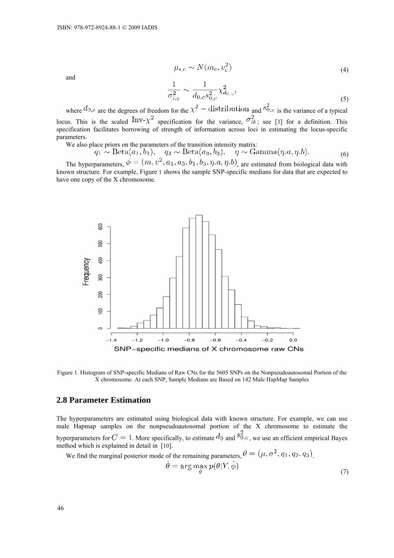
(4) and

(5)

where are the degrees of freedom for the and is the variance of a typical

locus. This is the scaled specification for the variance, ; see [3] for a definition. This specification facilitates borrowing of strength of information across loci in estimating the locus-specific parameters.

We also place priors on the parameters of the transition intensity matrix: (6) The hyperparameters, , are estimated from biological data with

known structure. For example, Figure 1 shows the sample SNP-specific medians for data that are expected to have one copy of the X chromosome.

Figure 1. Histogram of SNP-specific Medians of Raw CNs for the 5605 SNPs on the Nonpseudoautosomal Portion of the X chromosome. At each SNP, Sample Medians are Based on 142 Male HapMap Samples

2.8 Parameter Estimation

The hyperparameters are estimated using biological data with known structure. For example, we can use male Hapmap samples on the nonpseudoautosomal portion of the X chromosome to estimate the

hyperparameters for . More specifically, to estimate and , we use an efficient empirical Bayes method which is explained in detail in [10].

We find the marginal posterior mode of the remaining parameters, .

(7)

ISBN: 978-972-8924-88-1 © 2009 IADIS

46

When we have access to multiple samples we can use the EM aglorithm to find the posterior mode. Using the priors in Section 2.7, this leads to the following updates.

1. For each locus, , and copy number, , update given the other parameters by combining the normal population distribution for with the normal mixture distribution for the samples on locus :

(8)

2. For each locus, , and copy number, , update given the other parameters by combining the

population distribution for with the normal mixture distribuion for the samples on locus :

(9) In the applications to the data we used the method of moments procedure to estimate and .

Specific details are given in the data analyses section. One could use Markov chain Monte Carlo (MCMC) to estimate these parameters in a more optimal way. This is a focus of our current research.

Given the parameter estimates, we then use the Viterbi algorithm to calculate the most probable sequence of CN states,

(10)

2.9 Data Analyses

We analyzed data from a set of HapMap samples containing aberrant SNPs that have been experimentally verified by quantitative real-time PCR (qPCR) in a separate study [6]. For estimation of the parameters of the transition intensity matrix, we used the method of moments based on the human population data. was set to , was set to , and the expected length of an amplification was set to bps, resulting in an of . We used empirical Bayes methods to estimate the parameters of the emission distribution based on the titration data which have known biological structure.

For fitting the discrete-time HMM, we use the VanillaICE package with the default settings (see [9], for details), except that we set the emission distribution to be the same as the continuous-time model.

The results are presented in Table 1. Among the models the CHMM performed the best with 13 out of 14 SNPs called correctly. The discrete-time HMM was next with 11 out 14 SNPs called correctly.

Table 1. Predictions by Various HMMs on a Set of Aberrant SNPs that have been Experimentally Verified by qPCR. DHMM is the Discrete-time HMM. CHMM is the Continuous-Time HMM

SNP Chr Sample qPCR DHMM dChip CHMMSNP_A-1941019 13 NA10851 0.86 1.00 1.00 1.00SNP_A-4220257 8 NA10851 1.40 2.00 2.00 2.00SNP_A-2114552 22 NA10863 2.74 2.00 2.00 3.00SNP_A-1842651 17 NA10863 4.27 3.00 2.00 3.00SNP_A-4209889 3 NA12801 1.24 2.00 2.00 1.00SNP_A-2102849 8 NA10863 0.88 1.00 2.00 1.00SNP_A-2122068 8 NA10863 0.85 1.00 1.00 1.00SNP_A-1932704 7 NA10863 0.00 1.00 2.00 1.00SNP_A-1889457 8 NA10863 1.05 1.00 1.00 1.00SNP_A-4204549 8 NA10863 0.82 1.00 1.00 1.00SNP_A-2125892 22 NA12707 0.00 1.00 2.00 1.00SNP_A-2217320 22 NA12707 1.40 1.00 2.00 1.00SNP_A-2126506 17 NA12707 4.51 3.00 2.00 3.00SNP_A-1851359 17 NA12707 2.53 3.00 2.00 3.00


47

2.10 Results from a Simulation Study

CNV breakpoints were simulated from a heterogeneous HMM with a loss/gain frequency of 0.01, except in one region of CN polymorphism of length 1 Mb which had an elevated loss/gain frequency of 0.2. These breakpoints were simulated over a 140 Mb stretch, the length of chromosome 8, independently for 100 samples, and then were mapped onto the genomic locations corresponding to the observed SNP markers for the Affymetrix 500K Nsp chip. For each sample, this resulted in underlying copy number calls for 14,839 SNPs. With these simulated copy number calls, observed data were then simulated from the following hierarchical model.

1. For each copy number class and SNP ;

(a) sample

(b) sample

For and , sample . This was done for , ,

, and . These values were chosen to mimic estimates from the titration data which have known biological structure.

For estimation of each simulated data set, we used the method of moments to estimate the parameters of the transition intensity matrix based on the training data described in Section 2.4. was set to ,

was set to , and the expected length of an amplification was set to bps, resulting in an of . For the parameters of the emission distribution, we fixed the class means to

across all SNPs, and we estimated variances from the data. For comparison, we also employed a different approach using the EM algorithm in which SNP-specific parameters, shown in equations Error! Reference source not found. and Error! Reference source not found., are updated until convergence. Note that this approach uses information across the 100 samples to estimate the parameters.

We compared the results of these continuous-time HMMs to two other methods: GLAD [4] and CBS [7]. For GLAD, the default settings were used. GLAD provides output labels which correspond to loss/gain/diploid status for each SNP. For CBS, we post-processed the results by merging classes with predicted means within 0.25 of one another. Furthermore, the class with mean closest to zero was assigned the diploid class (normal class of two copies). The remaining classes were assigned to either gain or loss depending on whether their predicted class mean was larger or smaller than the diploid class.

The results are presented in Table 2. The discrete-time HMM performed the best in terms of detecting aberrant loci. The reason for this is that the transition probability matrix of the discrete-time HMM in VanillaICE is actually quite similar to that derived from the continuous-time HMM, the difference being that in CHMM , whereas in DHMM is fixed. The value used by the discrete-time HMM appears to be more optimal for this simulated data set.

Table 2. Prediction Results for the Simlution Study. The Second Column is the Misclassification Error Rate, the Third

Column is the True Positive Rate of Detection, and the Fourth Column is the True Negative Rate. These Error Rates are based on Averages Across the 100 Samples

Method Misclassification rate TPR TNR CHMM 0.42% 53.30% 99.99% CHMM.EM 0.17% 82.04% 99.98% GLAD 1.84% 64.12% 98.46% CBS 0.18% 81.43% 99.98% CHMM 0.24% 88.41% 99.90%

ISBN: 978-972-8924-88-1 © 2009 IADIS

48

3. CONCLUSION

In this paper we develop and apply a continuous-time Hidden Markov Model for the analysis of genotyping data, to infer regions of altered copy number. We use a number of previously published results to help specify priors for the Bayesian models underlying the HMM. The copy number analysis and databases are a novel development in the area of genomics, hence it is important for models to be flexible enough to enable novel discoveries. In particular the data analysis in this paper underlines the importance of developing a reliable estimation procedure for the parameters of the transition intensity matrix, as the results produced by the Viterbi algorithm are quite sensitive to the specification of these parameters. We are currently working on more sophisticated estimation procedures which would avoid the need for a training data set as is needed for the method of moments estimation. The continuous-time HMM framework we use is a more natural setting, compared to discrete-time HMMs, to develop new prior and parameter specification models. Our results indicate that our CHMM is already competitive with the specialized DHMM implementation for such data (a VanillaICE package) while allowing for a more consistent modeling framework.

Future work also includes extending the model to the analysis of multiple samples, with the ultimate goal of detecting copy number polymorphisms.

REFERENCES

[1] Henrik Bengtsson et al. Estimation and assessment of raw copy numbers at the single locus level. Bioinformatics, 24(6):759–767, 2008.

[2] The International HapMap Consortium. A second generation human haplotype map of over 3.1 million SNPs. Nature, 449:851–861, 2007.

[3] Andrew Gelman et al. Bayesian Data Analysis. Chapman and Hall, second edition, 2003. [4] Philippe Hupe et al. Analysis of array CGH data: from signal ratio to gain and loss of DNA regions. Bioinformatics,

20(18):3413–3422, 2004. [5] Ming Lin et al. dchipSNP: signficance curve and clustering of SNP-array-based loss-of-heterozygosity data.

Bioinformatics, 20(8):1233–1240, 2004. [6] Laura E MacConaill et al. Toward accurate high-throughput SNP genotyping in the presence of inherited copy

number variation. BMC Genomics, 8(211), 2007. [7] Adam B. Olshen et al. Circular binary segmentation for the analysis of array-based DNA copy number data.

Biostatistics, 5(4):557–572, 2004. [8] Sheldon M. Ross. Introduction to probability models. Academic Press, seventh edition, 2000. [9] Robert Scharpf. VanillaICE: Hidden markov models for the assessment of chromosomal alterations using high-

throughput SNP arrays. R vignette, 2008. [10] Gordon K. Smyth. Linear model and empirical bayes methods for assessing differential expression in microarray

experiments. Statistical Applications in Genetics and Molecular Biology, 3, 2004. [11] Susann Stjernqvist et al. Continuous-index hidden Markov modelling of array CGH copy number data.

Bioinformatics, 23(8):1006–1014, 20076. [12] George Zogopoulos et al. Germ-line DNA copy number variation frequencies in a large North American population.

Human Genetics, 122(3-4):345–353, 2007.


49

OUT-OF-CORE DATA HANDLING WITH PERIODIC PARTIAL RESULT MERGING

Sándor Juhász, Renáta Iváncsy Department of Automation and Applied Informatics Budapest University of Technology and Economics

Goldmann Gy. ter 3., Budapest, Hungary

ABSTRACT

Efficient handling of large amount of data is hindered by the fact that the data and the data structures used during the data processing do not fit into the main memory. A widely used solution for this problem is to use the partitioning approach, where the data set to be processed is split into smaller parts that can be processed in themselves in the main memory. Summarizing the results created from the smaller parts is done in a subsequent step. In this paper we give a brief overview of the different aspects of the partitioning approach, and seek for the most desirable approach to aggregate web log data. Based on these results we suggest and analyze a method that splits the original data set into blocks with equal sizes, and processes these blocks subsequently. After a processing step the main memory will contain the local result based on the currently processed block, that is merged afterwards with the global result of the blocks processed so far. By complexity analysis and experimental results we show that this approach is both fault tolerant and efficient when used in record-based data processing, if the results are significantly smaller than the original data, and a linear algorithm is available for merging the partial results. Also a method is suggested to adjust the block sizes dynamically in order to achieve best performance.

KEYWORDS

Out-of-core data processing, partitioning, efficient data handling with checkpoints

1. INTRODUCTION

Nowadays there are even more applications where the computer-based logging of the different events is a straightforward demand, such as web log files, telephone call records, public service company records and so on. In this way thousands and millions megabytes of raw data are generated daily providing an important raw material for business analysis, workflow optimization and decision support. However, handling such huge amount of data is much more demanding than merely recording them into a log file. While in such data handling tasks (aggregating, creating statistics etc.) the calculations are rather simple, the most important problem to face is the memory limitation, as during the execution the computational costs are usually significantly lower compared to the costs of the memory and I/O operations.

The first step of the most real-world data handling processes is preparing the data to fit the need of the following complex data processing algorithms. Such preprocessing task can be the filtering, data transformation, compression, or collecting derived data, such as generating statistics along different dimensions, joining related records from a log file, aggregating certain features of them. As these operations work on the complete large dataset their complexity should be kept as near as possible to linear in order to achieve a good efficiency.

A widely used solution to increase the efficiency of handling of out-of-core data is using a so-called partitioning approach (Savasere et al., 1995), where the data set that has to be processed is split into smaller blocks that themselves can be processed in the main memory. The aggregation of the results created during the processing of the smaller blocks is carried out in a subsequent step. In this paper we give a brief overview of the different aspects of the partitioning method, and investigate the most desirable solution for our problem, namely aggregating different fields of web log data. Based on these results we suggest and analyze a method, called Periodic Partial Result Merging, that splits the original data set into smaller data blocks with

ISBN: 978-972-8924-88-1 © 2009 IADIS

50

equal sizes, and processes these blocks subsequently in a way, that after processing each one, the main memory will contain the local result belonging to that block, and this local result is merged afterwards with the global result on the disk created from the blocks processed so far. We show that this approach provides fault tolerance by supporting a check pointing technique, produces a valid global result any time form the data processed so far, and at the same time it is efficient for record-based data processing in the cases, where the results are significantly smaller than the original data, and a linear algorithm is available for merging the partial results.

The most important benefits of our block-based algorithm include the following: • The original dataset is read only once from the disk. This is achieved by the linear partitioning, that

allows processing each record right as they arrive, without leaving any part of the task to a subsequent processing turn. It means that generating a new complete result is based only on the block being currently processed and on the results of the blocks processed previously.

• After each block a valid global sub-result is created. That means that the processing is complete regarding the data processed so far. This would not be the case, if the partitions were selected randomly or if the merging phase were a distinct final step of the whole process.

• The algorithm is free from memory bottlenecks, the full control over the memory consumption allows processing data files of any length.

• Similarly to nearly all partitioning algorithms our method can be well parallelized. Block-wise creation of a final result makes the complexity of the merging phase become quadratic,

because of the nature of the algorithm. Of course in order to process long files, the quadratic complexity of merging should be handled somehow. As, the size of the results is usually small compared to the size of the original data records, the coefficient of the quadratic part is small, which can be reduced further by choosing the block size well, thus we will show that the execution time of the merging task can be approximated by a linear complexity. We will give a simple method allowing setting the optimal block size automatically without any user intervention.

During our experiments we will compare our method to the “brute force” approach with eager memory use which is more efficient for short inputs, but suffers from serious limitations when processing large amount of data. We will also draw the attention to the fact that using our method makes the final complexity of the complete processing become independent from the complexity of the original algorithm creating the partial results when the original algorithm fulfills some constraints. Based on these facts we can draw the conclusion that under the later specified circumstances the time need of our algorithm is substantially linearly proportional to the number of the input records.

The organization of the paper is as follows. Section 2 gives an overview of the related work regarding the ouf-of-core data handling. Section 3 introduces our novel algorithm called Periodic Partial Result Merging. Section 4 contains complexity analysis, while Section 5 introduces the experiments done on real data files. We summarize our work in Section 6.

2. RELATED WORK

Efficient handling of large datasets that do not fit into the main memory is a challenging task because the I/O costs are significantly higher than that of the main memory accesses. For this reason different approaches are used to solve this problem. In this section we give a brief overview how large data is handled in the literature in a way that the data that has to be processed actually fit into the main memory. These main approaches are based on sampling, compression and partitioning.

If the result to be generated does not necessary have to be complete, the sampling method (Toivonen, 1996) (Zaki et al, 1997) can be used for creating an approximate result in the main memory. In this case, a well chosen, representative part of the whole dataset is read into the memory (using some heuristics to obtain a good sample), and the processing task is carried out on this small part of the data only. In some cases the results are verified with a subsequent read of the complete database (Lin. and Dunham,1998). The disadvantage of the method is that it does not create a complete result, thus it may not find all the necessary results or in case of aggregation like tasks the method obtains an approximate result only. Furthermore, the heuristics for the sampling phase is not trivial for all cases. The advantage of sampling is that it has to read the database only twice in worst case.


51

Another method for handling large datasets is to compress the original data, so that the compressed form fits into the memory. The subsequent steps generate the result based on the compressed form of the data (Han et al., 1999) (Grahne and Zhu. 2004). Of course not all dataset can be compressed to the necessary extent, thus this approach has to be combined with the other approaches mentioned in this section. A typical form of this solution is to use a compact data structure, such as a tree, for storing the data.

A widely used approach of out-of-core data handling is the partitioning method (Savasere et al., 1995). Here the input data is split into smaller blocks that fit into the memory, and the processing algorithm is executed on these parts of data successively. The main difference between the sampling and the partitioning is that in case of partitioning all the input records are used, that is, the union of the used blocks completely covers the original input dataset, so that all records are used once and only once. The partitions may contain subsequent or arbitrary grouped records. The processing task is executed on the distinct partitions, the results are written to the disk, and the global result, that is, the result based on the whole input dataset, is created in a subsequent step by a new disk read by merging the locally found results.

The way the local results can be used to generate a single global result is based on the way the local results are created. In some cases the global result is only the union of the local ones (Grahne and Zhu. 2004) (Nguyen et al., 2005) (Nguyen et al., 2006). In other cases a simple merging task has to be accomplished (Savasere et al., 1995) (Lin and Dunham, 1998) ,or another more complex algorithm has to be executed for generating the global result (Tang et al, 2005). For example for generating the maximal closed itemsets in itemset mining, for generating the global maximal closed itemsets all frequent itemsets have to be known, thus a further database read is needed for obtaining the final results (Lucchese et al, 2006)..

It is a particular task in case of partitioning algorithms to determine the size and the content of each partition. The trivial way is to split the input data into successively following parts of the same sizes (Savasere et al., 1995) (Lin and Dunham, 1998) (Lucchese et al, 2006). However, in some cases it is worth to do some extra work for reduce the complexity of the processing task. For example block creation based on clustering the records of the input file reduces the dependencies between the items of different blocks, thus it can accelerate the processing and the merging of the partitions significantly, or it can help to reduce the volume of the false result candidates (Nguyen et al., 2005) (Nguyen et al., 2006).

After introducing the state of the art of out-of-core data handling, in the next section we will suggest a novel partitioning method for this same purpose.

3. PERIODIC PARTIAL RESULT MERGING

The here introduced Periodic Partial Result Merging method uses a partition-based approach for processing data that does not fit into the main memory. The main purpose of developing this algorithm was to handle time-ordered log files continuously and efficiently in a web log mining project (Iváncsy and Juhász, 2007) .

The algorithm builds on the previously mentioned idea of splitting the input data set into subsequent blocks of equal size. The specialties of the approach are the following:

• In the basic version each block processing phase is followed by a merge phase. The reason for that is to periodically provide a global result for all the records that have been already processed. Furthermore this approach fits well the immediate processing of the newly generated records, and support easy implementation of pipeline based parallelism.

• The merging phase is facilitated using a hash table for storing the local and in a certain sense the global results as well. Hash tables are not only useful in creating the results (finding the correct aggregate structure for each record), but they also support fast merging of the partial results.

The solution presented in this paper expects a file containing a sequence of records as input. Each record has the same structure and length; the order and sizes of the fields in the record are identical. Although the input file is a series of logical related records, it is not necessary that these records are contained by a single file. While the algorithm executes the processing step on the blocks individually as usual (Savasere et al., 1995) , instead of storing each partial result on the disk and merging them after each block in a final step, our method merges the locally generated results with the global result created based on the blocks processed so far.

Periodic Partial Result Merging method splits the original input set of N records into S number of blocks containing the same amount of records (M records each, S = N/M). The size of the blocks has to be chosen

ISBN: 978-972-8924-88-1 © 2009 IADIS

52

arbitrary according the needs of the processing provided they fit into the main memory together with all the structures that are used during the processing step. These blocks are processed then one by one. During a block is processed an ordered local result is generated that is stored in the main memory. The size of this storage structure is estimated when calculating the size of the blocks. At the end of each iteration the memory-based local result is merged with the ordered global result created so far, which is stored on the disk. The merged new result is also written to the hard disk. The iterations are repeated continuously until all blocks are finished. An important advantage of this approach is that local results are never written to the disk, as merging is done from the memory, thus the disk only stores the different iterations of the global result.

The detailed steps of the Periodic Partial Result Merging algorithm and an illustration for the merging phase are depicted in Figure 1, while the notations used in the code are shown in Table 1. The example for merging is presented by using an aggregation (summing) operation.

Table 1. Notations and their Meaning Used in the Pseudo Code in Figure 1

Notation Meaning Bi The block i. RLi RGi RG RLi(j) RGi(j) |RGi|

The local result set generated from the block i. The global sub result set generated after processing the block i. The global result set The record j of the block i. The record j of the global result set after processing the block i. The size of the global result set after iteration i.

Figure 1. Pseudo Code of the Algorithm and Illustration of the Merging Step

It is important to note that ordering is a key feature to allow easy and linear merging of the partial results.

Normally this is done by a separate sorting operation with a complexity of m*log m preferring lower block sizes (m) as included in Figure 1 as well. Using hash tables provides an implicit ordering of records enforced by the storage structure itself, thus the cost of sorting is eliminated in our approach which place absolutely no restriction on the block sizes.

A further advantage of the method is that after each block we have a complete global result for all the records processed so far. Thus in case of a system crash only the processing step of the last block has to be repeated that was not finished before the system was down. This is supported by the feature of merging the global result with a disk to disk operation preserving the previous global result as well.


53

4. COMPLEXITY ANALYSIS

Our analysis of complexity is based on summarizing the cost of the two periodically repeated steps, namely the cost of generating the local result and that of the merging phase. Note, that we assume the existence of a method to store the local and the global results in an ordered manner and also an algorithm that allows the linear, pair by pair merging these two types of results (as shown above).Considering the huge amount of data the complexity analysis is accomplished separately regarding the number of disk accesses and the processing costs.

The disk complexity of the algorithm is calculated as follows. The disk usage cost kdisk is measured in records and has three components for each block: reading the input data, reading the global result produced in the previous step, and writing next iteration of global result. Assuming that processing x records of data generates αx amount of result (usually α«1), the cost of processing block j can be calculated using the following equation:

( ))jα(mmjjmmkkkkk jdiskjwriteresultjreadresultjreaddatajdisk 121)1()()()1()()( −+=+−+=++= − αα where m is the number of records found in one block. The I/O cost of the algorithm for the whole process

(where n/m=s is kept in mind): ( ) ( )

mnnsmmsjmmsjmkk

s

j

s

j

s

jjdiskdisk

αααα 22

111)( 12)12(1 +=+=−+==−+== ∑∑∑

===

From this equation we can draw the conclusion that the disk demand can be considered nearly linear when α is small enough (that is the processing algorithm creates an aggregated (compressed) result of the input data) and/or when the block size m is great enough.

The I/O independent part of the processing costs can be calculated by considering the processing complexity of the algorithm executed on each block, denoted by f(m), and considering the number of comparison steps when creating the global results. The number of the comparison steps after each block equals to the sum of the number of the local result records (mα) and the number of the global result records (mα(j-1)). The processing cost of the block j can be calculated as follows:

αββαα jmmfjmmmfk jproc +=−++= )())1(()()(

where β is a proportional factor to handle the two types of operation (processing step and the merging step) in the same manner.

The total cost of the whole process can be calculated as follows:

( )m

nmmfnm

mn

mn

mmfnmssmsfjmmfkk

s

j

s

jjprocproc 22

)(2

)(2

)1()()( 22

2

11)(

αβαβαβαβαβ +⎟⎠⎞

⎜⎝⎛ +=⎟⎟

⎠

⎞⎜⎜⎝

⎛++=

++=+== ∑∑

==

From the above formula we can see, that the complexity becomes quadratic independently of the original processing complexity f(m), and even the importance of the quadratic member is low when choosing a great block size, provided that the type of the processing step significantly reduces the volume of the results compared to the volume of the input records (α is small enough).

An important advantage of the method, as mentioned earlier, is that the partial processing is solved in a way, that at the end of every block it can be suspended, and restarted later again. This approach makes the algorithm fault tolerant, because the errors arising during the long processing time, and the unplanned halts do not require the system to process the whole data again from the beginning. Only the last, uncompleted block has to be processed again from its beginning.

Considering these facts we can draw the conclusion, that the method can be used efficiently when the disk demand of the global results is significantly smaller than that of the records from the result is created. In general in case of processing large datasets the prerequisite is fulfilled, because the main task is to derive well arranged, informative and compact data from the disordered, unmanageably large input.

Block-wise creation of a final result makes the complexity of the merging phase become quadratic due to the nature of the algorithm. It is important to note that this seems to be avoidable by applying a single merging step after producing all the local results as suggested in the literature. Unfortunately this approach has several drawbacks. It is not only the fact, that we loose the possibility of continuously having a global result but the method would not guarantee a better performance at all. First, it requires to write local results after each block to the disk, and then read them again at the end, which comes with extra (although linear) I/O costs. Secondly, and more important, that still the merging would not be linear as it is very unlikely to be

ISBN: 978-972-8924-88-1 © 2009 IADIS

54

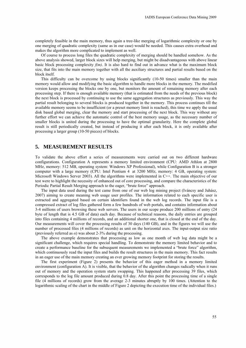
completely feasible in the main memory, thus again a tree-like merging of logarithmic complexity or one by one merging of quadratic complexity (same as in our case) would be needed. This causes extra overhead and makes the algorithm more complicated to implement as well.

Of course to process long files the quadratic complexity of merging should be handled somehow. As the above analysis showed, larger block sizes will help merging, but might be disadvantageous with above linear basic block processing complexity f(m). It is also hard to find out in advance what is the maximum block size, that fits into the main memory together with all the auxiliary structures and partial results based on the block itself.

This difficulty can be overcome by using blocks significantly (10-50 times) smaller than the main memory would allow and modifying the basic algorithm to handle more blocks in the memory. The modified version keeps processing the blocks one by one, but monitors the amount of remaining memory after each processing step. If there is enough available memory (that is estimated from the needs of the previous block) the next block is processed by continuing to use the same aggregation structures as previously. This way the partial result belonging to several blocks is produced together in the memory. This process continues till the available memory seems to be insufficient (or a preset memory limit is reached), this time we apply the usual disk based global merging, clear the memory and start processing of the next block. This way without any further effort we can achieve the automatic control of the best memory usage, as the necessary number of smaller blocks is united during the processing to have the optimal granularity. Here the complete global result is still periodically created, but instead of producing it after each block, it is only available after processing a larger group (10-50 pieces) of blocks.

5. MEASUREMENT RESULTS

To validate the above effort a series of measurements were carried out on two different hardware configurations. Configuration A represents a memory limited environment (CPU: AMD Athlon at 2800 MHz, memory: 512 MB, operating system: Windows XP Professional), while Configuration B is a stronger computer with a large memory (CPU: Intel Pentium 4 at 3200 MHz, memory: 4 GB, operating system: Microsoft Windows Server 2003). All the algorithms were implemented in C++. The main objective of our test were to highlight the necessity of enhanced out of core processing, and compare the characteristics of the Periodic Partial Result Merging approach to the eager, “brute force” approach.

The input data used during the test came from one of our web log mining project (Iváncsy and Juhász, 2007) aiming to create meaning web usage user profiles. The information related to each specific user is extracted and aggregated based on certain identifiers found in the web log records. The input file is a compressed extract of log files gathered form a few hundreds of web portals, and contains information about 3-4 millions of users browsing these web servers. The users in our scope produce 200 millions of entry (24 byte of length that is 4.5 GB of data) each day. Because of technical reasons, the daily entries are grouped into files containing 4 millions of records, and an additional shorter one, that is closed at the end of the day. Our measurements will cover the processing results of 30 days (140 GB), and in the figures we will use the number of processed files (4 millions of records) as unit on the horizontal axes. The input-output size ratio (previously referred as α) was about 2-3% during the processing.

The above example demonstrates that processing as low as one month of web log data might be a significant challenge, which requires special handling. To demonstrate the memory limited behavior and to create a performance baseline for the subsequent measurements we implemented a “brute force” algorithm, which continuously read the input files and builds the result structures in the main memory. This fact results in an eager use of the main memory creating an ever growing memory footprint for storing the results.

The first experiment (Figure 2) presents the behavior of this eager method in a memory limited environment (configuration A). It is visible, that the behavior of the algorithm changes radically when it runs out of memory and the operation system starts swapping. This happened after processing 39 files, which corresponds to the log file amount produced during 0.8 day. After this point the processing time of a single file (4 millions of records) grow from the average 2-3 minutes abruptly by 100 times. (Attention to the logarithmic scaling of the chart in the middle of Figure 2 depicting the execution time of the individual files.)


55

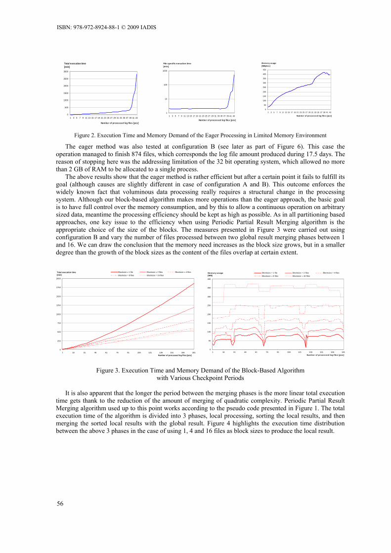
0

500

1000

1500

2000

2500

3000

1 3 5 7 9 11 13 15 17 19 21 23 25 27 29 31 33 35 37 39 41 43

Num ber of processed log files [pcs]

Total execution time[min]

1

10

100

1000

1 3 5 7 9 11 13 15 17 19 21 23 25 27 29 31 33 35 37 39 41 43

Num ber of processed log files [pcs]

File specific execution tim e[m in]

0

50

100

150

200

250

300

350

400

450

1 3 5 7 9 11 13 15 17 19 21 23 25 27 29 31 33 35 37 39 41 43

Num ber of processed log files [pcs ]

Mem ory usage[MBytes ]

Figure 2. Execution Time and Memory Demand of the Eager Processing in Limited Memory Environment

The eager method was also tested at configuration B (see later as part of Figure 6). This case the operation managed to finish 874 files, which corresponds the log file amount produced during 17.5 days. The reason of stopping here was the addressing limitation of the 32 bit operating system, which allowed no more than 2 GB of RAM to be allocated to a single process.

The above results show that the eager method is rather efficient but after a certain point it fails to fulfill its goal (although causes are slightly different in case of configuration A and B). This outcome enforces the widely known fact that voluminous data processing really requires a structural change in the processing system. Although our block-based algorithm makes more operations than the eager approach, the basic goal is to have full control over the memory consumption, and by this to allow a continuous operation on arbitrary sized data, meantime the processing efficiency should be kept as high as possible. As in all partitioning based approaches, one key issue to the efficiency when using Periodic Partial Result Merging algorithm is the appropriate choice of the size of the blocks. The measures presented in Figure 3 were carried out using configuration B and vary the number of files processed between two global result merging phases between 1 and 16. We can draw the conclusion that the memory need increases as the block size grows, but in a smaller degree than the growth of the block sizes as the content of the files overlap at certain extent.

0

50

100

150

200

250

300

350

400

1 16 31 46 61 76 91 106 121 136 151 166 181Number of processed log files [pcs]

Memory usage[MB]

Blocksize = 1 f ile Blocksize = 2 f iles Blocksize = 4 f iles

Blocksize = 8 f iles Blocksize = 16 f iles

Figure 3. Execution Time and Memory Demand of the Block-Based Algorithm

with Various Checkpoint Periods It is also apparent that the longer the period between the merging phases is the more linear total execution

time gets thank to the reduction of the amount of merging of quadratic complexity. Periodic Partial Result Merging algorithm used up to this point works according to the pseudo code presented in Figure 1. The total execution time of the algorithm is divided into 3 phases, local processing, sorting the local results, and then merging the sorted local results with the global result. Figure 4 highlights the execution time distribution between the above 3 phases in the case of using 1, 4 and 16 files as block sizes to produce the local result.

0 250 500 750

1000 1250 1500 1750 2000

1 16 31 46 61 76 91 106 121 136 151 166 181Number of processed log files [pcs]

Total execution time [min] Blocksize = 1 file Blocksize = 2 files Blocksize = 4 files

Blocksize = 8 files Blocksize = 16 files

ISBN: 978-972-8924-88-1 © 2009 IADIS

56

Blocksize = 1 file

0

4

8

12

16

1 17 33 49 65 81 97 113 129 145 161 177 193 209 225Number of processed log files [pcs]

File specific execution time[min]

Processing Sorting Merging

Blocksize = 4 files

0

4

8

12

16


File specific execution time[min] Processing Sorting Merging

Blocksize = 16 files

0

4

8

12

16


File specific execution time[min] Processing Sorting Merging

Figure 4. Distribution of the File Specific Execution Times Between the Processing Phases with Various Checkpoint Periods

Figure 5 and 6 compare the execution time and the memory demand of the eager and the periodic approaches for configuration A and B respectively. As the processing algorithms is inherently slow (processing the 30 days of data takes several days), the partial results are saved time to time to the disk in case of the eager method as well (checkpoint after each 16 files). We present here three versions of the Periodic Partial Result Merging algorithm. The first one is the basic method with a block size of 16 files. The second one is the automatic approach with adaptive block sizes where the memory limit was set to 512 MB. The third version contains a further optimization, with uses the ordering provided by the internal hash table instead of complete sorting explicitly (sorting is still needed, but only inside the slots of the hash table). It is clearly visible that automatic choice of the block sizes provides a comfortable way of gaining the best performance of the algorithm while preserving the full control over the memory consumption. The elimination of the sorting cost in this cases resulted in a further 5-6% performance gain.

0

100

200

300

400

500

600

700

800

1 8 15 22 29 36 43 50 57 64Number of processed log files [pcs]

Total execution time [min]

Eager method Block based (16 files)Adaptive (300 MB) Adaptive (300 MB) without sorting

0

50

100

150

200

250

300

350

400

450

1 8 15 22 29 36 43 50 57 64

Number of processed log files [pcs]

Memory[MB]

Eager method Block based (16 files)Adaptive (300 MB) Adaptive (300 MB) without sortingl

Figure 5. Execution Time and Memory Demand of the Different Algorithms in Memory Limited Environment

0

500

1000

1500

2000

2500

3000

3500

71 186 290 435 550 644 735 874

Number of processed log files [pcs]

Total execution time[min]

Adaptive [512 MB] without sorting Eager method

0

200

400

600

800

1000

1200

1400

1600

1800

2000

71 186 290 435 550 644 735 874Number of processed log files [pcs]

Memory[MB] Adaptive [512 MB] without sorting Eager method

Figure 6. Execution Time and Memory Demand of the Eager and the Best Block-Based Algorithm Using Configuration B

Figure 6 shows that where both methods work as they are supposed to Periodic Partial Result Merging is visibly (even by 50%) slower compared to the eager method. We pay this price for the increased amount of I/O operations (global results is periodically completely read and written back to the disk). Although in Figure 6 the quadratic complexity is still not apparent after 3300 minutes (55 hours) of execution, Figure 3 reminds, the optimization does not suppress this component totally. It is important to note that the memory limit of the adaptive algorithm was set to 512 MB, which is far less than the 2 GB the eager algorithm was allowed to use. Choosing the memory limit too high would cause the algorithm to run for long periods (here 55 hours) without writing out any result, which would considerably reduce the efficiency of check-pointing.


57

6. CONCLUSIONS AND FUTURE WORKS

When processing huge amount of data, it is important to control the memory handling of the algorithms by different methods. We have to seek for processing the highest amount of data possible in the memory, without the intervention of the virtual memory management of the operating system. In this paper we described and analyzed a partitioning-based approach called Periodic Partial Result Merging, and showed that under certain circumstances it shows a nearly linear behavior, while it provides a valid global result continuously during the processing and by its nature allows an easy check-pointing.

One of the most important questions in case of all partitioning methods is how to estimate the size of the blocks. In this paper we suggested a method how to adjust the block sizes dynamically by (logically) creating a number of smaller blocks as basic units and processing them in groups respecting the preset memory limit. This is allowed by continuously monitoring the memory allocation during the processing phase and when the available memory does not seem sufficient, the processing of the next block is postponed after the merging of the current partial result to the complete global result.

Another optimization suggested in this paper was to use hash tables to organize the partial results where possible as their provide a constant average access time to their elements, and also offer an implicit internal ordering of the partial and global results allowing the omit the explicit sorting phase.

Although it was not shown in the paper the algorithm is well suited for parallel processing either in data parallel, or in pipelined manner, but in this case it is harder to take advantage of the automatic choice of block sizes, and it is harder to organize the continuous presence of a valid global result.

ACKNOWLEDGEMENTS This work was completed in the frame of Mobile Innovation Centre’s integrated project Nr. 3.2. supported by the National Office for Research and Technology (Mobile 01/2004 contract).

REFERENCES

Benczúr A. A., Csalogány K., Lukács A. Rácz B. Sidló Cs., Uher M. and Végh L., Architecture for mining massive web logs with experiments, In Proc. of the HUBUSKA Open Workshop on Generic Issues of Knowledge Technologies

Grahne, G. Zhu J. 2004, Mining frequent itemsets from secondary memory, ICDM '04. Fourth IEEE International Conference on Data Mining, pp. 91-98.

Han, J., Pei, J., and Yin, Y. 1999 Mining frequent patterns without candidate generation. In Chen, W., Naughton, J., and Bernstein, P. A., editors, Proc. of ACM SIGMOD International Conference on Management of Data, pages 1-12.

Iváncsy, R. and Juhász, S. 2007, Analysis of Web User Identification Methods, Proc. of IV. International Conference on Computer, Electrical, and System Science, and Engineering, CESSE 2007, Venice, Italy, pp. 70-76.

Lin J. and Dunham M. H 1998., Mining association rules: Anti-skew algorithms, In 14th Intl. Conf. on Data Engineering, pp. 486-493.

Lucchese C, Orlando, S. and Perego, R., 2006, Mining frequent closed itemsets out of core. In SDM ’06: Proceedings of the third SIAM International Conference on Data Mining, April 2006.

Nguyen Nhu, S., Orlowska, M. E. 2005, Improvements in the data partitioning approach for frequent itemsets mining, 9th European Conference on Principles and Practice of Knowledge Discovery in Databases (PKDD-05), pp. 625-633.

Nguyen S. N. and Orlowska M. E. 2006, A further study in the data partitioning approach for frequent itemsets mining, ADC '06 Proceedings of the 17th Australasian Database Conference, pp. 31-37.

Salvatore C. L., Perego O. R. 2006, Mining frequent closed itemsets out-of-core, 6th SIAM International Conference on Data Mining, pp. 419-429.

Savasere A., Omiecinski E. and Navathe S. 1995, An efficient algorithm for mining association rules in large databases, VLDB '95: Proceedings of the 21th International Conference on Very Large Data Bases, pp. 432-444

Tang, P., Ning, L., and Wu, N. 2005. Domain and data partitioning for parallel mining of frequent closed itemsets. In Proceedings of the 43rd Annual Southeast Regional Conference - Volume 1 (Kennesaw, Georgia, March 18 - 20, 2005). ACM-SE 43. ACM, New York, NY, 250-255. DOI= http://doi.acm.org/10.1145/1167350.1167423

Toivonen H., 1996, Sampling Large Databases for Association Rules, Morgan Kauffman, pp. 134-145. Zaki, MJ, Parthasarathy, S., Li, W., and Ogihara, M. 1997, Evaluation of Sampling for Data Mining of Association Rules,

7th International Workshop on Research Issues in Data Engineering (RIDE--in conjunction with ICDE), pp 42-50, Birmingham, UK, April 7-8.

ISBN: 978-972-8924-88-1 © 2009 IADIS

58

A FUZZY WEB ANALYTICS MODEL FOR WEB MINING

Darius Zumstein, Michael Kaufmann Information Systems Research Group, University of Fribourg

Boulevard de Pérolles 90, 1700 Fribourg (Switzerland)

ABSTRACT

Analysis of web data and metrics has become a crucial task of electronic business to monitor and optimize websites, their usage and online marketing. First, this paper shows an overview of the use of web analytics, different web metrics measured by web analytics software like Google Analytics and other Key Performance Indicators (KPIs) of e-business. Second, an architecture of a fuzzy web analytics model for web usage mining is proposed to measure, analyze and improve website traffic and success. In a fuzzy classification, values of web data and metrics can be classified into several classes at the same time, and it allows gradual ranking within classes. Therefore, the fuzzy logic approach enables a more precise classification and segmentation of web metrics and the use of linguistic variables or terms, represented by membership functions. Third, a fuzzy data warehouse as a promising web usage mining tool allows fuzzy dicing, slicing and (dis)aggregation, and the definition of new query concepts like “many page views”, “high traffic period” or “very loyal visitors”. Fourth, Inductive Fuzzy Classification (IFC) enables a automated definition of membership functions using induction. This inferred membership degrees can be used for analysis and reporting.

KEYWORDS

Fuzzy classification, fuzzy logic, web analytics, web metrics, web usage mining, electronic business.

1. INTRODUCTION

Since the development of the World Wide Web 20 years ago, the Internet presence of companies has become a crucial instrument of information, communication and electronic business. With the growing importance of the web, the monitoring and optimization of a website and online marketing has become a central task too. Therefore, web analytics and web usage mining gain in importance for both business practice and academic research. Web analytics helps to understand the traffic on the website and the behavior of visitors.

Today, many companies are already using web analytics software like Google Analytics to collect web data and analyze website traffic. They provide useful dashboards and reports with important metrics to the responsible persons of the website, marketing or IT. Like web analytics software, a data warehouse is an often-used information system for analysis and decision making purposes.

So far, classifications of web metrics or facts in data warehouses have always been done in a sharp manner. This often leads to inexact evaluations. This paper shows a fuzzy logic approach applied to web analytics, where classification of metrics yields a gradual degree of membership in several classes.

After an introduction to web analytics in section 2, section 3 proposes a process and an architecture of a web analytics model with seven layers. Section 4 explains the fuzzy classification approach and discusses two fuzzy induction methods for web usage mining. Section 5 gives a conclusion and an outlook.

2. WEB ANALYTICS

According to the Web Analytics Association (2009), web analytics is the measurement, collection, analysis and reporting of Internet data for the purposes of understanding and optimizing web usage. Phippen et al. (2004) quote the Aberdeen Group by defining web analytics as the monitoring and reporting of website usage so that enterprises can better understand the complex interactions between web site visitor actions and website offers, as well as leverage insight to optimise the site for increased customer loyalty and sales.


59

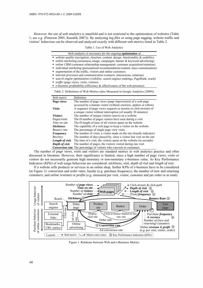
Legend: Metric-ratio (rate) Key Performance Indicators (KPIs) Web metric

Reach

Basket

Conversion rate

Order rate

Usa

ge b

ehav

ior

of v

isito

rs

Basket-to-buy rate

Order

Purchase frequency& recency

Number of page viewsTime on site

Number of visitors Number of visits

Product site

Entry page

Web pages

Exit page

Bounce Rate

Search engines

Bookmarks,URL entries

Online advertising

Ad conversion rate

Clic

k ra

te

Online revenue & profit(e.g. per visit, visitor, order)

External links

Click-to-basket rate

Stickiness

Ad

clic

k

rate

Purc

hase

beh

avio

r of

onl

ine

cust

omer

s

Number of (new and returning) customers

Click-stream & click-path Depth of visit Length of visit (Visit) frequency

Display click rate

However, the use of web analytics is manifold and is not restricted to the optimization of websites (Table 1; see e.g. (Peterson 2005, Kaushik 2007)). By analyzing log files or using page tagging, website traffic and visitors’ behaviour can be observed and analyzed exactly with different web metrics listed in Table 2.

Table 1. Use of Web Analytics

Web analytics is necessary for the ongoing optimization of … website quality (navigation, structure, content, design, functionality & usability) online marketing (awareness, image, campaigns, banner & keyword advertising) online CRM (customer relationship management: customer acquisition/retention) individual marketing (personalized recommendation/content, mass customization) segmentation of the traffic, visitors and online customers internal processes and communication (contacts, interactions, relations) search engine optimization (visibility, search engines rankings, PageRank, reach) traffic (page views, visits, visitors) e-business profitability (efficiency & effectiveness of the web presence)

Table 2. Definitions of Web Metrics (also Measured in Google Analytics (2009))

Web metric Definition Page views The number of page views (page impressions) of a web page

accessed by a human visitor (without crawlers, spiders or robots) Visits A sequence of page views requests (a session or click-stream) of

a unique visitor without interruption (of usually 30 minutes) Visitors The number of unique visitors (users) on a website Pages/visits The Ø number of pages visitors have seen during a visit Time on site The Ø length of time of all visitors spent on the website Stickiness The capability of a web page to keep a visitor on the website Bounce rate The percentage of single page view visits Frequency The number of visits, a visitor made on the site (loyalty indicator) Recency The number of days passed by, since a visitor last visit on the site Length of visit The time of a visit, the visitors spent on the website (in seconds) Depth of visit The number of pages, the visitors visited during one visit Conversion rate The percentage of visitors who converts to customers

The number of page views, visits and visitors are standard metrics in web analytics practice and often discussed in literature. However, their significance is limited, since a high number of page views, visits or visitors do not necessarily generate high monetary or non-monetary e-business value. As Key Performance Indicators (KPIs) of web usage behaviour are considered: stickiness, visit, depth of visit and length of visit.

If a website sells products or services in an online shop, further KPIs of e-business have to be considered (in Figure 1): conversion and order rates, loyalty (e.g. purchase frequency), the number of new and returning customers, and online revenues or profits (e.g. measured per visit, visitor, customer and per order or as total).

Figure 1. Relations between Web and e-Business Metrics

ISBN: 978-972-8924-88-1 © 2009 IADIS

60

3. WEB ANALYTICS MODEL

3.1 Web Analytics Process

The selection of web metrics and KPIs always depends on the strategy and objectives of a website. Different metrics and KPIs have to be measured to analyse, for instance, a news website, an e-commerce site, a support website, a blog or a community website. Therefore, the web analytics process starts with the task of identifying and defining the main goals and KPIs of a website. The collection, preparation and analysis of web data belong to the website, integration and data layer of the web analytics model (compare Figure 2).

Within the data warehouse and web mining layer, a web metric system is modelled and implemented by a data warehouse, which handles and classifies integrated web data fuzzily. On the presentation layer, query results, reports and dashboards are provided to analysts. They and managers of IT, marketing or accounting analyze and control website-related results, and they plan and act activities to optimize e-business success.

3.2 Website & Data Layer

In the domain of web analytics, two technical methods are mainly used to analyse website traffic: server-site and client-side data collection. Server-site data collection methods extract and analyse data out of the log files ( in Figure 2). However, server-side methods do not measure web traffic exactly, because of the caching in web browsers and proxy servers and due to requests of search engines crawlers or robots. In addition, page views and visitors can not be identified distinctly with log files, and events (like mouse clicks) are recorded neither. Finally, log files extractions and reporting are complicated and time-consuming, particularly, if multiple websites or several web servers are used. As result, it has become less important.

Using client-site data collection or page tagging ( ), data about the visitor and each page view is send to a tracking server by a JavaScript code (or a one-pixel tag) inserted in each (X)HTML page. If a website is built with a Content Management System (CMS; ), the JavaScript snippet can be embedded easily.

With the client-side data collection method, all visits and all actions of a visitor on every web page can be tracked exactly (i.e. each mouse click and all keyboard entries), as well as technical information about the visitor (e.g. size/resolution of the screen; type/language of the used browser or system). Further advantages are that JavaScript is not allowed to be cached by proxies or browsers, and crawlers of search engines do not read it. Google, WebTrends, Nedstat and many other companies provide web analytics software using page tagging. Google Analytics (2009) is the most used freeware and well documented by books (Clifton 2008).

However, from an e-business point of view, not only click-stream data about the visitor(s) is interesting, but especially customer-related information about online orders, the purchase history, payment behaviour, customer profile, and so on. Data of Customer Relationship Management (CRM; ) is stored in operational data bases. To ensure a holistic view of online customers, data from various sources has to be cleaned, transformed and consolidated in a data preparation step, before it is integrated to a data warehouse ( ).

3.3 Data Warehouse & Web Mining Layer

For analysis and reporting purposes, web and online customer data is loaded into a Data Warehouse (DWH; ). A DWH is defined as a multidimensional, subject-oriented, integrated, time-varying, non-volatile

collection of data in support of the management’s decision-making process (Inmon et al. 2008). A DWH is a promising tool for web analytics, since facts like page views or online revenues can be analysed and aggregated over different dimensions like website, visitor and time ( ). Another strength of DWH is the possibility to provide user- and context-relevant information using slicing and dicing.

Slicing, dicing, drill-down and roll-up (i.e. dis-/aggregation) based on the fuzzy logic approach discussed in the following section, enable the definition of linguistic variables and extended dimensional concepts. For example, new classification concepts like “high traffic period” (e.g. in the evening or at the weekend), “many page views” (of a web page or of a visitor), “very loyal visitors” (with high visit or purchase frequency) or “high value customers” (with high online revenues) can be defined and queried by data analysts.


61

It is proposed by Fasel and Zumstein (2009) to define fuzzy classes, dimensions, linguistic variables and the membership degrees of the fuzzy data warehouse by meta data (meta fuzzy table). This method is more flexible than other approaches and it fulfils the additional requirements of a DW 2.0 (Inmon et al. 2008).

Figure 2. Architecture of the web analytics model

Additionally, a fuzzy DWH is also a powerful basis for web usage mining ( ). Web usage mining is a part of web mining, beside web structure and web content mining (Liu 2007, Markov & Larose 2007). It refers to discovery and analysis of patterns in click-streams and associated data collected or generated as a result of user interactions with web resources on one or more websites (Mobasher 2007).

In this paper, web usage mining is considered as the application of data mining techniques like fuzzy classification or fuzzy clustering to web analytics in order to detect, analyse or query promising segments of website traffic, and of visitor or customer behaviour. As shown in section 4.2, inductive fuzzy classification allows the automated calculation of probabilities based on membership degrees for reporting and analysis.

This method can improve predictive web analytics ( ), as well as predictive analytics in online and individual marketing, as Kaufmann and Meier (2009) show in a case study.

Dashboards

Identification: Login IP address Cookies

Presentation layer

Integration layer

Data layer

Website layer

External web data

(Google Analytics, eTracker, WebTrends, Omniture, etc.)

Customer data base

Otherdata bases

Customer & e-commerce data

Webpage 1

Webpage 2

Webpage n

Page Tagging<script type="text/ javascript"> var gaJsHost =(("https… </script>

Visits

Order

Client-side data collection

Server-side data collection

Purchase history

Profile

Application Programming Interface (API)

Standard dashboards

Fuzzy data warehouse Web analytics system

Implementation Modelling Strategies & goals of the website & e-business

Web metrics system (cause-and-effect-chain)

Web metrics, e.g. Page views Visits Visitors New visitors Pages/visits Time on Site Stickiness Depth of visit Purchase frequency & recency Revenues Conversion rates

Dimension time

Dim

ens.

visi

tor

Page

1

Page

2

Page

3Pa

ge n

Day Y

Visitor X

Facts

Dimensions (operations:

slicing, dicing, aggregation)

Met

a da

ta (m

eta

fuzz

y ta

bles

) Visitor

…

Queries Results

Reports

Accounting

Managementlayer

eMarketing

IT

Data warehouse layer

CMS

Web mining laye r

Inductive fuzzy classification

Analyze Plan Act Control

Web usage mining

Data preparation

Internal web data

Predictive web analytics

CRM software

Web analyticstracking server

Logfiles

Dimension web page

Fact (page views)

ISBN: 978-972-8924-88-1 © 2009 IADIS

62

3.4 Presentation & Management Layer

On the presentation layer, content- or user-specific queries, reports and dashboards are prepared and presented by analysts to the responsible person(s) of the IT, marketing or accounting department and to the management board ( ), who plans and decides about website-related activities to optimize the website ( ).

4. FUZZY WEB ANALYTICS

4.1 Fuzzy Classification of the Web Metric Page Views

The theory of fuzzy sets and fuzzy logic goes back to Lofti A. Zadeh in 1965. It takes the subjectivity, imprecision, uncertainty and vagueness of human thinking and language into account, and expresses it with mathematical membership functions. A fuzzy set can be defined formally as follow (Zimmermann 1992, Meier et al. 2008, Werro 2008): if X is a set, then the fuzzy set A in X is defined in (1) as

A = x,μA a( )( ){ } (1)

where x ∈ X, µA : X → [0, 1] is the membership function of A and µA (x) ∈ [0, 1] is the membership degree of x in A.

Figure 3. Sharp (a) and Fuzzy (b) Classification of the Web Metric Page Views

For example, in a sharp set (Figure 3a), the terms “few”, “medium” or “many” of the linguistic variable page views can be either true (1) or false (0). A value of 1 of the membership function µ (Y-axis in Figure 3a) means that the number of page views (on the X-axis) is corresponding to one set. A value of 0 indicates that a given number of page views do not belong to one of the sets. The number of page views of a visitor per month are defined as “few” between 0 and 32, 33 to 65 page views are “medium” and more than 66 are classified as “many” page views. However, to classify page views – or any other web metric – sharply, is problematic near the classification boundaries, as following examples shows. If visitor 1 has 65 page views, he is classified in the “medium” class, visitor 2 with 70 has “many” page views. Although the two visitors have visited nearly the same number of pages (visitor 2 visited only 5 pages more), they are assigned to two different sets, or classes respectively. By defining fuzzy sets (Figure 3b), represented by the membership functions, there are continuous transitions between the terms “few”, “medium” and “many”. Fuzzily, the number page views of visitor 1 are classified both as “medium” (0.55 resp. 55%) and “many” (0.45 resp. 45%). Also visitor 2 belongs partly to two classes (60% to “many” and 40% to “medium”) at the same time.

Obviously, the use of fuzzy classes allows a more precise classification of web metric values, and risks of misclassifications can be reduced. The fuzzy classification of KPIs like online revenue, profit or conversion rates is especially pertinent, since their valuations usually have far-reaching consequences for e-business.

4.2 Inductive Fuzzy Classification for Web Usage Mining

Web usage mining is a data mining method to recognize patterns in web site navigation by web site visitors (Spiliopoulou 2000, Srivastava et al. 2000). A common web usage mining task is the analysis of associations between visited pages (Escobar-Jeria et al. 2007). Two inductive fuzzy classification methods are proposed

Visitor 1

µ 1

0

µ 1

0.40

0.60

0.45 0.55

few medium many

Visitor 1 Visitor 2

Visitor 2

0

few medium many

Page views (per month) 0 10 20 30 40 50 60 70 80 90

a) b)

0 10 20 30 40 50 60 70 80 90 100 100 Page views (per month)


63

here to discover knowledge about web usage patterns. Inductive Fuzzy Classification (IFC) is the process of grouping elements into a fuzzy set whose membership function is inferred by induction from data (Kaufmann and Meier 2009). First, Inductive Fuzzy Classification by Percentile Rank (IFC-PR) generates fuzzy membership functions to common linguistic terms like “low”, “medium” and “high” for the number of page views. Second, Inductive Fuzzy Classification by Normalized Likelihood Ratios (IFC-NLR) can be applied to infer a membership function of a web page in a target page (like a product or order page).

4.2.1 Motivation for the Proposed Methods The two methods for IFC proposed in this paper use simple probabilistic measures such as percentile ranks and likelihood ratios for generating fuzzy membership functions. The aim is to apply this fuzzyfication in web data analysis for knowledge discovery, reporting, and prediction, which has several advantages. First, most data mining methods are dichotomous in nature, especially classification. As proposed by Zimmermann (1997), fuzzy classification methods become appropriate when class membership is supposed to be gradual. Thus the advantage of fuzzy classification in web mining is the possibility to rank web pages by a gradual degree of membership in classes. Second, the results of knowledge discovery are often not directly understandable by human decision makers (Mobasher 1997). The advantage of fuzzy logic based methods is that the generated models (i.e. membership functions) are easy to interpret. In fact, using simple probabilistic measures with a clear semantic make the membership functions more understandable and thus suitable for human decision support. Third, not only does the IFC methods provide gradual rankings that are easily interpretable, but also these fuzzy classifications can be derived and defined from data automatically, by induction. Consequently, they are suitable for the application to web usage mining.

4.2.2 Web Usage Mining with IFC-PR In web usage mining, the importance of web pages is measured by the number of page views per page. This number alone does not have much meaning. Only the context of the number in relation to the number of views of other pages provides valuable knowledge. Fuzzy classification is used here to put the number of web page views in a linguistic context (i.e. the use of linguistic terms like “low”, “medium” and “high”).

The IFC-PR method is proposed here to induce the membership functions to these linguistic terms automatically, using the sampled probability distribution (P) of values, which is defined as follows: For a metric M, the empirical percentile rank of a value x determines the membership to the fuzzy class “high” (2):

μhigh x( ):= P M < x( ) (2)

For M, the classification as being “low” (formula 3) is the negation of the membership to the class “high”:

μlow x( ):=1− μhigh x( ) (3)

For a web metric M, the classification as being “medium” is defined by the following formula (4):

μmedium x( ):=1− abs μhigh x( )− 0.5( )− abs μlow x( )− 0.5( ) (4)

For example, web page 1 (W1) has 1035 visits per month. To classify this number, the distribution of the number of visits per page is used. Assume, 56 of 80 pages have less visits than W1. Thus, the calculation is:

μhigh visit W1( )( ):= P Number of visits < visits W1( )( )=5680

= 0.7 (5)

Therefore, the fuzzy classification of the visits per month for the web page W1 being “high” is 0.7. The fuzzy classification for the linguistic term “low” is 0.3, and for “medium” it is 0.6.

4.2.3 Web Usage Mining with IFC-NLR For web usage mining it is interesting to know which web pages (page X) are visited together with a target page such as the online shop (target page Y). Therefore, a fuzzy classification for each web page is calculated with a degree of membership to the target page. That type of fuzzy classification indicates the degree of association in web usage between two web pages. To analyze the influence of an analytic variable X to a target variable Y in terms of fuzzy classification, the IFC-NLR method is applied to calculate the membership degree of values x ∈ dom(X) in the values y ∈ dom(Y). Thus, the values of the target variable

ISBN: 978-972-8924-88-1 © 2009 IADIS

64

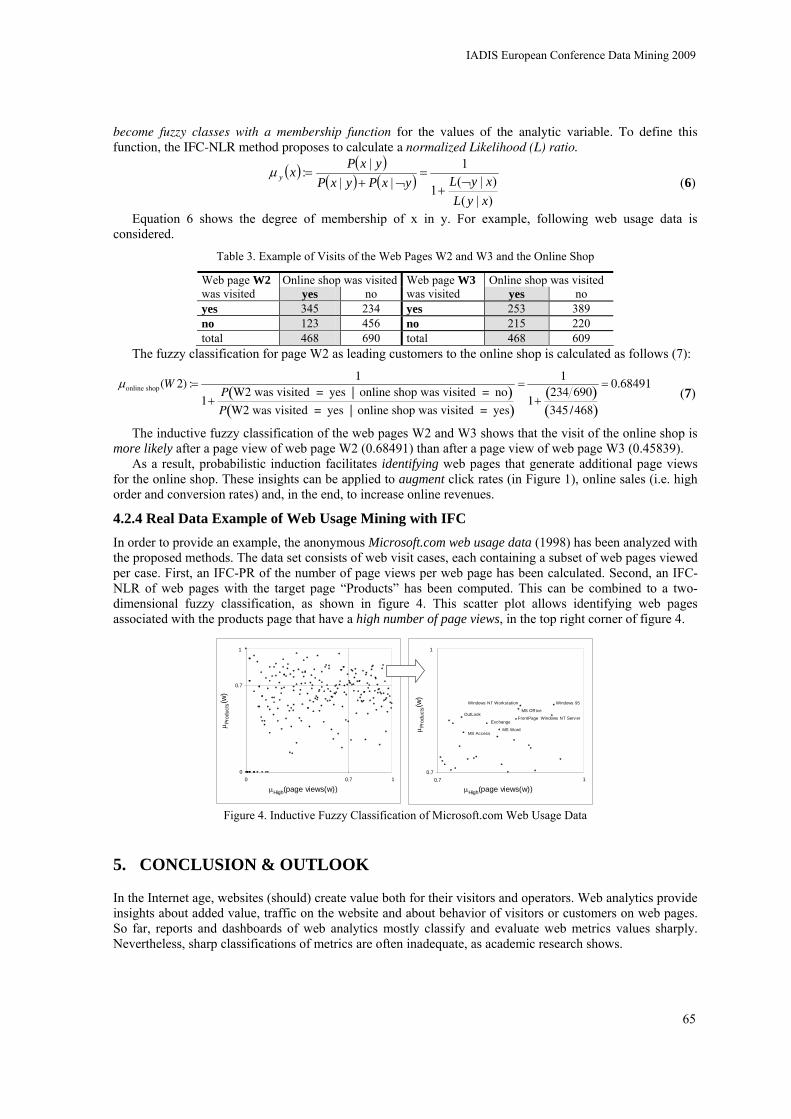
become fuzzy classes with a membership function for the values of the analytic variable. To define this function, the IFC-NLR method proposes to calculate a normalized Likelihood (L) ratio.

( ) ( )( ) ( )

)|()|(

1

1||

|:

xyLxyLyxPyxP

yxPxy ¬

+=

¬+=μ

(6)

Equation 6 shows the degree of membership of x in y. For example, following web usage data is considered.

Table 3. Example of Visits of the Web Pages W2 and W3 and the Online Shop

Online shop was visited Online shop was visited Web page W2 was visited yes no

Web page W3 was visited yes no

yes 345 234 yes 253 389 no 123 456 no 215 220 total 468 690 total 468 609

The fuzzy classification for page W2 as leading customers to the online shop is calculated as follows (7):

μonline shop(W 2) :=1

1+P W2 was visited = yes | online shop was visited = no( )P W2 was visited = yes | online shop was visited = yes( )

=1

1+234 690( )345 /468( )

= 0.68491

(7)

The inductive fuzzy classification of the web pages W2 and W3 shows that the visit of the online shop is more likely after a page view of web page W2 (0.68491) than after a page view of web page W3 (0.45839).

As a result, probabilistic induction facilitates identifying web pages that generate additional page views for the online shop. These insights can be applied to augment click rates (in Figure 1), online sales (i.e. high order and conversion rates) and, in the end, to increase online revenues. 4.2.4 Real Data Example of Web Usage Mining with IFC In order to provide an example, the anonymous Microsoft.com web usage data (1998) has been analyzed with the proposed methods. The data set consists of web visit cases, each containing a subset of web pages viewed per case. First, an IFC-PR of the number of page views per web page has been calculated. Second, an IFC-NLR of web pages with the target page “Products” has been computed. This can be combined to a two-dimensional fuzzy classification, as shown in figure 4. This scatter plot allows identifying web pages associated with the products page that have a high number of page views, in the top right corner of figure 4.

Figure 4. Inductive Fuzzy Classification of Microsoft.com Web Usage Data

5. CONCLUSION & OUTLOOK

In the Internet age, websites (should) create value both for their visitors and operators. Web analytics provide insights about added value, traffic on the website and about behavior of visitors or customers on web pages. So far, reports and dashboards of web analytics mostly classify and evaluate web metrics values sharply. Nevertheless, sharp classifications of metrics are often inadequate, as academic research shows.

0

0.7

0 0.7

μ Prod

ucts

(w)

mProducts(w)

0.70.7

μHigh(page views(w))

μ Prod

ucts

(w)

1

11

Windows 95Windows NT Workstation

Windows NT Serv er

MS Off ice

FrontPage

1

OutLook

Exchange

MS WordMS Access

μHigh(page views(w))


65

Therefore, this paper proposes a fuzzy web analytics model to overcome the limitations of sharp data handling in data warehouses and web usage mining. In a fuzzy classification, elements can belong to several classes at the same with a gradual membership degree. In addition, inductive fuzzy classification provides methods to define these membership degrees automatically. The advantage of the fuzzy methods is that they provide a gradual ranking of web metrics induced by data suitable for web manager decision support. A real data example showed how to present the knowledge discovered by web usage mining graphically.

The architecture of the proposed fuzzy web analytics model provides a theoretical framework to master the huge amount of Internet data companies are confronted with. To proof the discussed web analytics model, real web data of e-business practice has to be analyzed in future studies. In addition, further case studies with companies are planned, to show the advantages and limitations of the fuzzy classification approach.

The research center Fuzzy Marketing Methods (www.FMsquare.org) applies the fuzzy classification to data base technologies and online marketing. It provides several open source prototypes, for example, the fuzzy Classification Query Language (fCQL) toolkit, which allows fuzzy queries and the calculation of the membership degree of data stored in MySQL or PostgreSQL data bases.

REFERENCES & FURTHER READING

Clifton, B., 2008: Advanced Web Metrics with Google Analytics, Wiley, New York, USA. Escobar-Jeria, V. H., Martín-Bautista, M. J., Sánchez, D., Vila, M., 2007: Web Usage Mining Via Fuzzy Logic

Techniques. In: Melin, P., Castillo, O., Aguilar, I. J., Kacprzyk, J., Pedrycz, W. (Eds.), 2007: Lecture Notes In Artificial Intelligence, Vol. 4529, Springer, New York, USA, pp. 243-252.

Fasel, D., Zumstein, D., 2009: A Fuzzy Data Warehouse for Web Analytics, In: Proceedings of the 2nd World Summit on the Knowledge Society (WSKS 2009), September 16-18, Crete, Greece.

Galindo, J. (Ed.), 2008: Handbook of Research on Fuzzy Information Processing in Databases, Idea, Hershey, USA. Google Analytics, 2009: http://www.google.com/analytics (accessed 12th of May 2009). Inmon, W., Strauss, D., Neushloss, G., 2008: DW 2.0 – The Architecture for the Next Generation of Data Warehousing,

Elsevier, New York, USA. Kaufmann, M., Meier, A., 2009: An Inductive Fuzzy Classification Approach applied to Individual Marketing, In:

Proceedings of the 28th North American Fuzzy Information Processing Society Annual Conference, Ohio, USA. Kaushik, A., 2007: Web Analytics, Wiley, New York, USA. Liu, B., 2007: Web Data Mining – Exploring Hyperlinks, Contents, and Usage Data, Springer, New York, USA. Markow, Z., Larose, D., 2007: Data Mining the Web, Wiley, New York, USA. Meier, A., Schindler, G., Werro, N., 2008: Fuzzy Classification on Relational Databases, In: (Galindo 2008, pp.586-614). Microsoft web usage data, 1998: http://archive.ics.uci.edu/ml/databases/msweb/msweb.html (accessed 12th of May 2009). Mobasher B., Cooley R., Srivastava J. 1997: Web Mining: Information and Pattern Discovery on the World Wide Web,

In Proc. of the 9th IEEE International Conf. on Tools with Artificial Intelligence (ICTAI'97). Mobasher, B., 2007: Web Usage Mining, In: (Liu 2007, pp. 449-483). Phippen, A., Sheppard, Furnell, S., 2004: A practical evaluation of Web analytics, Internet Research, Vol.14, pp.284-93. Peterson, E., 2005: Web Site Measurement Hacks, O’Reilly, New York, USA. Spiliopoulou, M, 2000: Web usage mining for web site evaluation. Communication of the ACM, Vol. 43, pp. 127–134. Srivastava, J., Cooley, R., Deshpande, M., Tan, P.-N., 2000: Web Usage Mining: Discovery and Application of Usage

Patterns from Web Data, In: ACM SIGKDD, Vol. 1, Is. 2, pp.1-12. Waisberg, D., Kaushik, A., 2009: Web Analytics 2.0: Empowering Customer Centricity, In: SEMJ.org, Vol. 2, available:

http://www.semj.org/documents/webanalytics2.0_SEMJvol2.pdf (accessed 12th of May 2009). Web Analytics Association, 2009: http://www.webanalyticsassociation.org/aboutus (accessed 12th of May 2009). Weischedel, B., Huizingh, E., 2005: Website Optimization with Web Metrics: A Case Study, In: Proceedings of the 8th

international conference on Electronic commerce (ICEC’06), August 14-16, Fredericton, Canada, pp. 463-470. Werro, N., 2008: Fuzzy Classification of Online Customers, Dissertation, University of Fribourg, Switzerland, available:

http://ethesis.unifr.ch/theses/downloads.php?file=WerroN.pdf (accessed 12th of May 2009). Zadeh, L. A., 1965: Fuzzy Sets. In: Information and Control, Vol. 8, pp. 338-353. Zimmermann, H.-J., 1992: Fuzzy Set Theory and its Applications, Kluwer, London, England. Zimmermann, H.-J., 1997: Fuzzy Data Analysis. In: Computational Intelligence: Soft Computing and Fuzzy-Neuro

Integration with Applications; Kaynak, O., Zadeh, L. A., Turksen, B., Rudas, I. J. (Eds.), Springer, New York, USA.

ISBN: 978-972-8924-88-1 © 2009 IADIS

66

DATE-BASED DYNAMIC CACHING MECHANISM

Christos Bouras, Vassilis Poulopoulos Research Academic Computer Technology Institute, N. Kazantzaki, Panepistimioupoli and

Computer Engineering and Informatics Department, University of Patras 26504 Rion, Patras, Greece

Panagiotis Silintziris

Computer Engineering and Informatics Department, University of Patras 26504 Rion, Patras, Greece

ABSTRACT

News portals based on the RSS protocol are becoming nowadays one of the dominant ways that Internet users follow in order to locate the information they are looking for. Search engines, which operate at the back-end of a big portion of these web sites, receive millions of queries per day on any and every walk of web life. While these queries are submitted by thousands of unrelated users, studies have shown that small sets of popular queries account for a significant fraction of the query stream. A second truth has to do with the high frequency that a particular user tends to submit the same or highly relative search requests to the engine. By combining these facts, in this paper, we design and analyze the caching algorithm deployed in our personalized RSS portal, a web-based mechanism for the retrieval, processing and presentation in a personalized view of articles and RSS feeds collected from major Internet news portals. By using moderate amounts of memory and little computational overhead, we achieve to cache query results in the server, both for personalized and non-personalized user searches. Our caching algorithm operates not in a stand-alone manner but it co-operates and binds with the rest of the modules of our Portal in order to accomplish maximum integration with the system.

KEYWORDS

Query results caching, search engine, personalized search, query locality, data retrieval, date-based caching.

1. INTRODUCTION

The technological advances in the World Wide Web combined with the low cost and the ease of access to it from any place in the world has dramatically changed the way people face the need for information retrieval. More and more users migrate from traditional mass media to more interactive digital solutions such as Internet news portals. As the number of users exponentially increases and the volume of data involved is high, it is very important to design efficient mechanisms to enable search engines to respond fast to as many queries as possible. One of the most common design solutions is to use caching, which may improve efficiency if the cached queries occur in the near future.

Regarding earlier classic works in the topic of caching, Markatos investigated the effectiveness of caching for Web search engines (Markatos E.P. 2001). The reported results suggested that there are important efficiency benefits from using caches, due to the temporal locality in the query stream. Xie and O’Hallaron also found a Zipf distribution of query frequencies (Xie and Halaron, 2002), where different users issue very popular queries, and longer queries are less likely to be shared by many users. On cache management policies, Lempel & Moran (Lempel and Moran, 2003) proposed one that considers the probability distribution over all queries submitted by the users of a search engine. (Fagni et al. 2006) described a Static Dynamic Cache (SDC), where part of the cache is read-only or static, and it comprises a set of frequent queries from a past query log. The dynamic part is used for caching the queries that are not in the static part. Regarding locality in search queries, in their earlier works, Jansen & Spink (Jansen and Spink, 2006) provide insights about short-term interactions of users with search engines and show that there is a great amount of locality in the submitted requests. Teevan et al. (Teevan et al. 2006) examined the search behaviour of more than a hundred anonymous users over the course of one year. The findings were that across the year, about


67

one third of the user queries were repetitions of queries previously issued by the same user. Although these studies have not focused on caching search engine results, all of them suggest that queries have significant locality, which particularly motivates our work.

In our work, we take advantage of this space and time locality, and we cache the results from very recently used queries in order to reduce the latency on the client and the database-processing load from the server. Because of the fact that the caching is server side, both registered and unregistered users of the portal can take benefit. Furthermore, for registered users, the algorithm takes into account the dynamic evolution of their profile and provides them with results even more close to their preferences and interests. The rest of the paper is structured in the following way: in the next section description of the architecture of the system with the focus in the algorithm of caching is presented. The caching algorithm is analyzed in Section 3. In section 4, we present some of the experimental results and evaluation of our work, regarding algorithmic performance, results accuracy and storage space requirements. We conclude in Section 5 with some remarks about the described techniques and future.

2. ARCHITECTURE

The architecture of the system is distributed and based on standalone subsystems but the procedure to reach at the desired result is actually sequential, meaning by this that the data flow is representative of the subsystems of which the mechanism consists. Another noticeable architectural characteristic is the existence of modularity throughout the system’s lines. This section is a description of how these features are integrated into the mechanism. We are putting the focus on the subsystem responsible for caching, though analysis of the other modules is presented in order to cross-connect the features of our system.

Figure 1. Search Module Architecture

The general procedure of the mechanism is as follows: first web pages are captured and useful text is extracted from them. Then, the extracted text is parsed followed by summarization and categorization. Finally we have the presentation of the personalized results to the end user. For the first step, a simple web crawler is deployed, which uses as input the addresses extracted from the RSS feeds. Theses feeds contain the web links to the sites where the articles exist. The crawler fetches only the html page, without elements such as referenced images, videos, CSS or JavaScript files. Thus, the database is filled with pages ready for input to the 1st level of analysis, during which, the system isolates the “useful” text from the html source. Useful text contains the article’s title and main body. This procedure analysis can be found in (self reference). In the 2nd level of analysis, XML files containing the title and the body of articles are received as input, targeting at applying pre-processing algorithms on this text in order to provide as output the keywords, their location in the text together with their absolute frequency in it. These results are the primary key to the 3rd level of analysis. In the 3rd level of analysis, the summarization and categorization technique takes place. Its main scope is to characterize the articles with a label (category) and come up with a summary of it. This procedure is described in (self reference).

ISBN: 978-972-8924-88-1 © 2009 IADIS

68

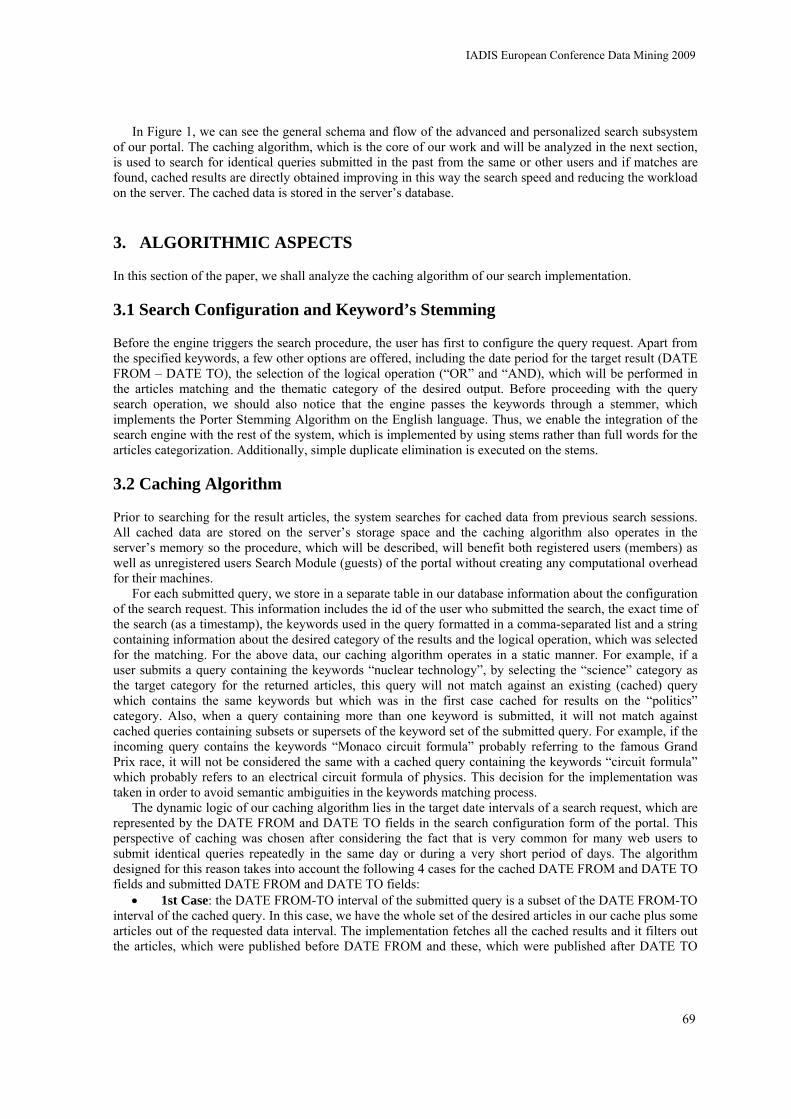
In Figure 1, we can see the general schema and flow of the advanced and personalized search subsystem of our portal. The caching algorithm, which is the core of our work and will be analyzed in the next section, is used to search for identical queries submitted in the past from the same or other users and if matches are found, cached results are directly obtained improving in this way the search speed and reducing the workload on the server. The cached data is stored in the server’s database.

3. ALGORITHMIC ASPECTS

In this section of the paper, we shall analyze the caching algorithm of our search implementation.

3.1 Search Configuration and Keyword’s Stemming

Before the engine triggers the search procedure, the user has first to configure the query request. Apart from the specified keywords, a few other options are offered, including the date period for the target result (DATE FROM – DATE TO), the selection of the logical operation (“OR” and “AND), which will be performed in the articles matching and the thematic category of the desired output. Before proceeding with the query search operation, we should also notice that the engine passes the keywords through a stemmer, which implements the Porter Stemming Algorithm on the English language. Thus, we enable the integration of the search engine with the rest of the system, which is implemented by using stems rather than full words for the articles categorization. Additionally, simple duplicate elimination is executed on the stems.

3.2 Caching Algorithm

Prior to searching for the result articles, the system searches for cached data from previous search sessions. All cached data are stored on the server’s storage space and the caching algorithm also operates in the server’s memory so the procedure, which will be described, will benefit both registered users (members) as well as unregistered users Search Module (guests) of the portal without creating any computational overhead for their machines.

For each submitted query, we store in a separate table in our database information about the configuration of the search request. This information includes the id of the user who submitted the search, the exact time of the search (as a timestamp), the keywords used in the query formatted in a comma-separated list and a string containing information about the desired category of the results and the logical operation, which was selected for the matching. For the above data, our caching algorithm operates in a static manner. For example, if a user submits a query containing the keywords “nuclear technology”, by selecting the “science” category as the target category for the returned articles, this query will not match against an existing (cached) query which contains the same keywords but which was in the first case cached for results on the “politics” category. Also, when a query containing more than one keyword is submitted, it will not match against cached queries containing subsets or supersets of the keyword set of the submitted query. For example, if the incoming query contains the keywords “Monaco circuit formula” probably referring to the famous Grand Prix race, it will not be considered the same with a cached query containing the keywords “circuit formula” which probably refers to an electrical circuit formula of physics. This decision for the implementation was taken in order to avoid semantic ambiguities in the keywords matching process.

The dynamic logic of our caching algorithm lies in the target date intervals of a search request, which are represented by the DATE FROM and DATE TO fields in the search configuration form of the portal. This perspective of caching was chosen after considering the fact that is very common for many web users to submit identical queries repeatedly in the same day or during a very short period of days. The algorithm designed for this reason takes into account the following 4 cases for the cached DATE FROM and DATE TO fields and submitted DATE FROM and DATE TO fields:

• 1st Case: the DATE FROM-TO interval of the submitted query is a subset of the DATE FROM-TO interval of the cached query. In this case, we have the whole set of the desired articles in our cache plus some articles out of the requested data interval. The implementation fetches all the cached results and it filters out the articles, which were published before DATE FROM and these, which were published after DATE TO


69

attribute of the submitted request. The server’s cache is not updated with new articles because in this case no search is performed in the articles database.

• 2nd Case: the DATE FROM of the submitted query is before the DATE FROM of the cached query and the DATE TO of the submitted query is after the TO DATE TO of the cached query. In this case, the desired articles are a superset of the articles, which are cached in the database. As a consequence, the algorithm fetches all the cached results but it also performs a new search for articles in the date intervals before and after the cached date interval. When the search procedure finishes, the algorithm updates the cache by extending it to include the new articles and by changing the DATE FROM and DATE TO attributes so that they can be properly used for future searches.

• 3rd Case: the DATE FROM of the submitted query is before the DATE FROM of the cached query and the DATE TO of the submitted query is between the DATE FROM and DATE TO of the cached query. In this case, a portion of the desired articles exists in the cache. The algorithm first fetches all the results and then it filters out the articles, which are after the DATE TO date of the submitted request. Furthermore, a new search is initiated for articles not existing in the cache memory. For the new search the DATE FROM and DATE TO dates become the DATE FROM date of the submitted query and the DATE FROM date of the cached query.

• 4th Case: The form case is similar to the third case but in the opposite date direction. The final results consist of the cached results between DATE FROM date of the submitted request, the DATE TO date of the cached request and the new articles coming from a new search between the DATE TO date of the cached query and the DATE TO date of the submitted query.

We should notice that for the cached results data, an expiration mechanism is deployed. Every cached query is valid for a small number of days, in order to keep the engine’s output to the end user as accurate as possible. Whenever a search for a matching with the cached results is performed, cached date that have expired are deleted from the database and are replaced with new ones. It is also possible for the same query to exist more than one cached records as long as they have not expired. The selection of the proper expiration time for the cached data will be discussed in section 5 of the paper.

By examining the cache matching algorithm, operating in the server machines, we can see that in all four cases, we achieve to limit the computational overhead of a fresh search in the database by replacing it with some overhead for cached results filtering. However, this filtering is implemented with simple XML parsing routines and cannot be considered as a heavy task for the server. The most significant improvement happens in the first case, where no new search is performed and all the results are fetched directly from the cache. This is a great benefit to our method as this is the most common case, where the user submits the same query over and over without changing the DATE FROM and DATE TO date fields or by shrinking the desired date borders. The worst case is the second, where the user expands his query in both time directions (before and after) in order to get more results in the output. In this case, the engine has to perform two new searches, followed by an update query in the database cache. However, this is the rarest case, as the average user tends to shrink the date interval rather than expanding it, when he repeatedly submits an identical query in order to get more date-precise and date-focused results. In the other two situations, one new search is executed each time and one update is committed in the database. This means that in an average case, we can save more than 50% of our computational overhead when the expansion of the date borders (with the newly submitted query) are not bigger than the cached results date interval.

4. EXPERIMENTAL EVALUATION

In our experiment to evaluate the caching algorithm, which was described in the previous section, we create a virtual user to submit queries to the server. The executed queries consist of keywords from several thematic categories (sports, science, politics, etc) used throughout the articles database of our system. We choose to test caching performance on queries containing no more than three keywords, in order for the output to contain a big number of articles and for the overall procedure to last as much as needed for our time measurements to be sufficient and capable of analysis and conclusions.

ISBN: 978-972-8924-88-1 © 2009 IADIS

70

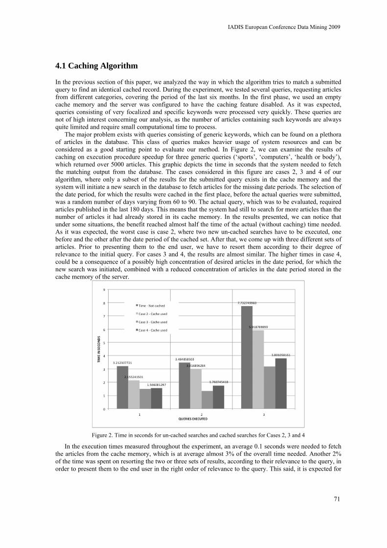
4.1 Caching Algorithm

In the previous section of this paper, we analyzed the way in which the algorithm tries to match a submitted query to find an identical cached record. During the experiment, we tested several queries, requesting articles from different categories, covering the period of the last six months. In the first phase, we used an empty cache memory and the server was configured to have the caching feature disabled. As it was expected, queries consisting of very focalized and specific keywords were processed very quickly. These queries are not of high interest concerning our analysis, as the number of articles containing such keywords are always quite limited and require small computational time to process.

The major problem exists with queries consisting of generic keywords, which can be found on a plethora of articles in the database. This class of queries makes heavier usage of system resources and can be considered as a good starting point to evaluate our method. In Figure 2, we can examine the results of caching on execution procedure speedup for three generic queries (‘sports’, ‘computers’, ‘health or body’), which returned over 5000 articles. This graphic depicts the time in seconds that the system needed to fetch the matching output from the database. The cases considered in this figure are cases 2, 3 and 4 of our algorithm, where only a subset of the results for the submitted query exists in the cache memory and the system will initiate a new search in the database to fetch articles for the missing date periods. The selection of the date period, for which the results were cached in the first place, before the actual queries were submitted, was a random number of days varying from 60 to 90. The actual query, which was to be evaluated, required articles published in the last 180 days. This means that the system had still to search for more articles than the number of articles it had already stored in its cache memory. In the results presented, we can notice that under some situations, the benefit reached almost half the time of the actual (without caching) time needed. As it was expected, the worst case is case 2, where two new un-cached searches have to be executed, one before and the other after the date period of the cached set. After that, we come up with three different sets of articles. Prior to presenting them to the end user, we have to resort them according to their degree of relevance to the initial query. For cases 3 and 4, the results are almost similar. The higher times in case 4, could be a consequence of a possibly high concentration of desired articles in the date period, for which the new search was initiated, combined with a reduced concentration of articles in the date period stored in the cache memory of the server.

Figure 2. Time in seconds for un-cached searches and cached searches for Cases 2, 3 and 4

In the execution times measured throughout the experiment, an average 0.1 seconds were needed to fetch the articles from the cache memory, which is at average almost 3% of the overall time needed. Another 2% of the time was spent on resorting the two or three sets of results, according to their relevance to the query, in order to present them to the end user in the right order of relevance to the query. This said, it is expected for


71

the case 1 of our algorithm to achieve an almost 95% speed up on the search. After the first execution of these queries, every next submission of the same request is serviced in under 0.1 seconds. Whenever results are cached for a query, every following identical one which demands articles inside the date period of the cached result, will be processed in almost zero time – only the time needed to fetch the results from the cache - no resorting is required in this case as we have only one already sorted set of articles. This reduces the computational overhead on the server for time demanding queries to the cost of the search procedure for only the first time they are executed. Every next time they are processed through the cache memory and the algorithm operating on it.

4.2 Cache Memory Size

Our second concern was to examine how the number of the cached articles per query in our cache, affects the overall algorithm performance and the size of the database table used to store the cached data. We executed a generic query for several numbers of cached articles by increasing each time the date period in which the caching occurred. The total number of articles for this query was 4782 over a period of 4 months. For this experiment, we tested cases 2,3 and 4 of our algorithm, so that in every submitted request, a part of the results were not contained in the cache and the engine could not rely only on the cached data to create the output.

Figure 3. How the number of cached articles affects the speedup of a new search

From the graphical representation of Figure 3, relating the percentage of execution time speedup with the percentage of cached results on total results, we can notice that the search execution time reduces at an average 50% when a little less than 40% of the output has been cached. As the total number of articles in this test covered a period of four months, we can say, by statistic, that the 40% of the results would be retrieved by a search in a period of less than two months, which, speaking modestly, is a rather limited date interval on a common search. By that, it is meant that if a user submitted a search query, requesting articles for a period of more than two months, then every next time he submits an identical request, it would take at most half the time to be processed. If we add to this the fact that the algorithm updates the cache memory with new results, every time an extended (in terms of dates) version of an already cached query is submitted (the percentage of cached results probably increases and never decreases in every search), we could get even more improved execution times.

Due the fact that the algorithm stores for each query in the cache a limited set of information relative to the retrieved articles, such as ids, dates and relevance factors, the size of the cache per record in the server memory is kept at minimum. As an example, for caching the 4782 results of the above query, which is a rather generic one with a lot of articles to be found relative, the corresponding row size in the cache database table was measured to be less than 150KB. If we combine the small row size with the periodical deletion of

ISBN: 978-972-8924-88-1 © 2009 IADIS

72

cached query records that expire, the technique can guarantee low storage space requirements in the server. The selection of the expiration date will be discussed in the next paragraph.

4.3 Expiration Date and Result Accuracy

In the last phase of the experiment, we will examine the impact of selecting a proper expiration time for the cached records on the accuracy and the quality of the final output to the end user. As it was mentioned in the previous paragraph, the proposed algorithm periodically deletes cached records from the corresponding table in the database. The implementation of such an expiration mechanism in the algorithm is essential not only because it helps in keeping the storage space of the server’s cache low, but mainly for keeping the accuracy and the quality of the search results at high levels.

Our purpose in this last step of the experiment is to examine how extending the expiration time of the cached records degrades the accuracy of the output result. For this reason, we created a virtual user and constructed a profile for him with favourite thematic categories and keywords. Having no cached data for this user on the first day of the experiment, we had him submit several queries to the system and we cached the results for some of these queries. For the next days of the month, we had the user navigating inside the system by submitting every day several different queries, this time, without caching any of them or expanding the already existing cached results. Among the submitted queries, we included queries identical to the cached ones for comparison to be feasible. The personalization mechanism the portal takes into account the daily behavior of each registered user (articles he reads, articles he rejects, time spent on each article) and dynamically evolves the profile of the user. For example, it is possible for a user to choose the sports as his favorite category upon his registration, but he may occasionally show an increased interest over science related news. The personalization system then evolves his profile and starts feeding him with scientific news among the sport news and this evolution has an obvious impact in his search sessions inside the system.

Figure 4. How extending date expiration affects results accuracy

In figure 4, we can see how is the accuracy of the search result degraded over the days passing when comparing the actual search results with the cached ones. For our virtual user, on the first day, the average accuracy is obviously 100% as it is the day that the actual queries are cached. Every next day, we get the results (uncached) of the actual queries, which have relevance over 35% to the submitted requests, and we count at average, how many of them existed in the cached queries results. As time passes, the output of the actual queries change (according to the user’s evolving profile) and the average percentage of the cached results in the actual output decreases. Until the tenth day of the experiment, we can see that the accuracy is close to 90% to the actual results. However, after the first two weeks the accuracy is degraded at 70% and toward the end of the third week, it is close to 55%. In other words, if the user were to be presented, at this point, with the cached results (cached on the first day), instead of the actual results for his queries, he would see almost, only half of the results that match his changed (since first day) profile.


73

As a conclusion, caching the results of a search for more than two weeks is not a preferable solution for a registered user, as it might significantly produce invalid results, not matching his evolving profile and preferences. However, for unregistered users (guests) of the system, for whom no profile has been formed, an extended expiration date could be used. In our implementation, there is a distinction for registered and unregistered users when checking for cached data, which makes the caching algorithm more flexible.

5. CONCLUSION AND FUTURE WORK

Due to the dynamism of the Web, the content of the web pages change rapidly, especially when discussing about a mechanism that fetches more than 1500 articles on a daily basis and presents them personalized back to the end user. Personalized portals offer the opportunity for focalized results though, it is crucial to create accurate user profiles. Based on the profiles that are created from the mechanism we created a personalized search engine for our web portal system in order to enhance the searching procedure of the registered and the non-registered. In this paper, we discussed about the caching algorithm of the advanced search sub-system. We presented the algorithmic procedure that we follow in order to cache the results and how to utilize the cache in order to enhance the speed of the searching procedure. Finally, we described experimental procedures that prove the aforementioned enhancement in speed. Comparing the results to the generic search’s results it is obvious that the system is able to enhance the searching procedure and help the users locate the desired results quicker. For the future what we would like to do is to further enhance the whole system with a more accurate search personalization algorithm supporting “smarter” caching of data in order to make the whole procedure faster and in order to omit any results that are of very low user interest.

REFERENCES

Beitzel S. M., Jensen E. C., Chowdhury A., Grossman D. A. and Frieder O., 2004. Hourly analysis of a very large topically categorized web query log. ACM SIGIR, pp. 321-328.

Bouras C., Poulopoulos V., Tsogkas V. 2008. PeRSSonal's core functionality evaluation: Enhancing text labeling through personalized summaries. Data and Knowledge Engineering Journal, Elsevier Science, 2008, Vol. 64, Issue 1, pp. 330 - 345

DMOZ. Open directory project. http://www.dmoz.com Fagni, T., Perego, R., Silvestri, F., Orlando, S., 2006. Boosting the performance of Web search engines: Caching and

prefetching query results by exploiting historical usage data. ACM Transactions on Information Systems 24, pp. 51–78.

Google. Google Search Engine. http://www.google.com (last accessed March 2009) Jansen B. J., Spink A., 2006. How are we searching the World Wide Web? A comparison of nine search engine

transaction logs. Information Processing and Management, 42(1) ,pp. 248-263. Lempel, R., Moran, S., 2003. Predictive caching and prefetching of query results in search engines. Proceedings of the

12th WWW Conference, pp. 19–28 Markatos, E.P., 2001. On caching search engine query results. Computer Communications 24, pp. 137–143. Teevan J., Adar E., Jones R. and Pott M., 2006. History repeats itself: Re-peat queries in Yahoo’s logs. ACM SIGIR, pp.

703-704. Xie, Y., O’Hallaron, D.R., 2002. Locality in search engine queries and its implications for caching. IEEE Infocom 2002,

pp. 1238 – 1247. Yahoo. Yahoo Web Search. http://www.yahoo.com (last accessed March 2009)

ISBN: 978-972-8924-88-1 © 2009 IADIS

74

GENETIC ALGORITHM TO DETERMINE RELEVANT FEATURES FOR INTRUSION DETECTION

Namita Aggarwal VIPS, Guru Gobind Singh Indraprastha University, Delhi

R K Agrawal

School of Computer & Systems Science, Jawaharlal Nehru University, New Delhi

H M Jain Trinity College, Guru Gobind Singh Indraprastha University, Delhi

ABSTRACT

Real time identification of intrusive behavior based on training analysis remains a major issue due to high dimensionality of the feature set of intrusion data. The original feature set may contain irrelevant or redundant features. There is need to identify relevant features for better performance of intrusion detection systems in terms of classification accuracy and computation time required to detect intrusion. In this paper, we have proposed a wrapper method based on Genetic Algorithm in conjunction with Support Vector Machine to identify relevant features for better performance of intrusion detection system. To achieve this, a new fitness function for Genetic Algorithm is defined that focuses on selecting the smallest set of relevant features which provide maximum classification accuracy. The proposed method provides better result in comparison to the other commonly used feature selection techniques.

KEYWORDS

Feature selection, Support Vector Machine, Intrusion Detection, Genetic Algorithm.

1. INTRODUCTION

In last two decades, networking and Internet technologies have undergone a phenomenal growth. This has exposed the computing and networking infrastructure to various risks and malicious activities. The need of the hour is to develop strong security policies which satisfy the main goals of security (Hontanon, 2002) i.e. data confidentiality, data integrity, user authentication and access control, and availability of data and services. The most important factor in all these is the identification of any form of activity as secure or abusive. Intrusion detection is the art of detecting these malicious, unauthorized or inappropriate activities.

Intrusion Detection Systems (IDS) have been broadly classified into two categories (Lee, 1999): misuse detection and anomaly detection. Misuse detection systems identify attacks which follow well-known patterns. Anomaly detection systems are those which have the capability to raise alarms in case of patterns showing deviations from normal usage behavior. Various data mining techniques have been applied to intrusion detection because it has the advantage of discovering useful knowledge that describes a user’s or program’s behavior from large audit data sets. Artificial Neural Network (Cho and Park, 2003; Lippmann and Cunningham, 2000), Rule Learning (Lazarevic et al., 2003), Outlier Detection scheme (Han and Cho, 2003), Support Vector Machines (Abraham, 2001; Sung and Mukkamakla, 2003), Multivariate Adaptive Regression Splines (Banzhaf et al., 1998) and Linear Genetic Programming (Mukkamala et al., 2004) are the main data mining techniques widely used for anomaly and misuse detections. Most of the research has been carried out on the kddcup DARPA data.

The real time accurate identification of intrusive behavior based on training analysis remains a major issue due to the high dimensionality of the kddcup data (http://kdd.ics.uci.edu/databases/kddcup99/kddcup99.html). Although the data has 41 attributes, not all of them may contribute to the identification of a given attack. In fact, the presence of irrelevant and redundant


75

features may deteriorate the performance of the classifier and requires high computation time and other resources for training and testing the data. Hence, in order to make the classifier accurate and efficient we need to identify a set of relevant features for better performance of IDS.

But feature selection techniques, though extensively studied and widely employed for many real time applications, have been used scarcely in the intrusion detection domain. Hyvarinen et al. (2001) used PCA/ICA to compress data which did not yield satisfactory feature reduction from an intrusion detection perspective. Sung and Mukkamala (2003) have determined a smaller set of 19 features for intrusion detection task without compromising the performance in terms of classification accuracy. Chebrolu et al. (2004) determined a subset of 12 features and 17 features using feature selection algorithm involving Bayesian networks and, Classification and Regression trees respectively. In this paper, we have proposed a new fitness function for Genetic algorithm to identify relevant feature subset. The proposed method selects the smallest set of relevant features that provides maximum classification accuracy. In order to check the efficacy of proposed method for feature selection, we have compared our experimental results with other commonly used feature selection methods in machine learning and data mining.

In Section 2, the various feature selection techniques are discussed. Section 3 deals with proposed approach to identify relevant features for intrusion detection. Section 4 briefly describes Multi-class SVM. Section 5 gives the detailed description of the experimental setup and results. Finally the conclusions and the future work are discussed in Section 6.

2. FEATURE SELECTION TECHNIQUES

High dimensional features describing real life data in general contains noisy, irrelevant and redundant features which makes them inefficient for machine learning. So it becomes important to identify a small subset of relevant features to improve the efficiency and performance of learning algorithms. Thus, the removal of the noisy, irrelevant, and redundant features is a challenging task. There are two major approaches to overcome this: feature selection and feature extraction (Devijver and Kittler, 1982). While feature selection reduces the feature set by eliminating the features inadequate for classification, feature extraction methods build a new feature space from the original features. In literature, feature selection techniques are classified into two categories: filter methods and wrapper methods (Kohavi, and John, 1997; Langley, 1994). The Filter model depends on general characteristics of the training data to select a feature set without involving any learning algorithm. Most filter methods have adopted some statistical feature selection to determine relevant feature subset which requires less computation time.

The feature selection algorithm used for feature subset selection cannot be exhaustive. Hence one has to compromise with suboptimal solution. However the choice of criterion for evaluating the feature subsets is a sensitive issue. It has to estimate the usefulness of a subset accurately and economically. In literature, various suboptimal feature selection search techniques are suggested. Among them, the simplest method of constructing a subset of relevant feature is to select d individually best features present in original feature set. Features are ranked based on some statistical properties of given data. Information gain, Gini index and Relief-F are few most commonly used approaches for evaluating the ranking of features.

2.1 Information Gain

The Information Gain is a measure based on entropy which is popularized in machine learning by Quinlan (1986). It measures the decrease of the weighted average impurity of the partitions compared with the impurity of the complete set of examples. Expected information needed to classify a given sample is calculated by

)log(),...,,1

2 ss

ssssI(s i

m

i

im1 ∑

=

−= (1)

Where si (i=1, 2,…,m) represents samples of class i and s is the total number of samples in the training set.

ISBN: 978-972-8924-88-1 © 2009 IADIS

76

A feature F with values { f1, f2, …, fv } can divide the training set into v subsets { S1, S2, …, Sv } where Sj is the subset which has the value fj for feature F. Assuming Sj contain sij samples of class i, entropy of the feature F is given by

),...,(...

)( 11

1mjj

v

j

mjj ssIs

ssFE ∑

=

++= (2)

Information gain for feature F can be calculated as Gain(F) = I(s1, …, sm) – E(F) (3)

2.2 Gini Index

The Gini index is another popular measure for feature selection in the field of data mining proposed by Breiman et al. (1984). It measures the impurity of given set of training data and can be calculated as

Gini Index = {nl* GiniL + nr * GiniR}/n (4)

andGiniLwherek

i l

i

nL∑

=⎟⎟⎠

⎞⎜⎜⎝

⎛−=

1

2

0.1 ∑=

⎟⎟⎠

⎞⎜⎜⎝

⎛−=

k

i r

i

nRGiniR

1

2

0.1

GiniL and GIniR are Gini Index on the left and right side of the hyperplane respectively. Li and Ri are number of values that belong to class i in left and right partition respectively, nl and nr are number of values in left and right partition respectively, k is the total number of classes, n is the total number of expression values.

2.3 Relief-F

Relief algorithm (Kira and Rendell, 1992) is a feature selection method based on feature estimation. Most of the feature estimators are unable to detect any form of redundancy as the features are valued individually. However, Relief does not formulate conditional independence of features and hence captures their interdependencies and makes Relief a suitable choice for the task at hand. Relief assigns a positive weight to those features which have different values on pairs that belong to different classes and negative weight to those features that have different values on pairs that belong to the same class. Relief randomly selects one tuple and finds its nearest neighbors: one from the same class and the other from the different class. It computes the importance measure of every feature using these neighbors. Relief is limited to two-class problem and cannot deal with noisy and incomplete data whereas its extension by Robnik and Kononenko (2003) is more robust and can deal with noisy, incomplete and for multi-class problem.

The disadvantage of ranking method is that the features may be correlated among themselves (Ding and Peng, 2003). Sequential forward feature selection is another simple bottom up search approach used in literature where one feature at a time is added to the current subset of relevant features. The relevance of feature subset can be measured in terms of some distance metrics i.e. interclass distance, probabilistic distance etc. Most commonly used metrics in literature are: Euclidean distance, Mahalanobis distance and Inter-Intra distance.

2.4 Euclidean Distance

In this method, we are trying to find a subset of features X, for which X ⊂ Y, where Y is the entire feature set. The subset X is chosen such that it optimizes some criterion J. J(x) can be easily calculated as:

J(x) = max{(μi − μj)'(μi − μj)} (5) For all classes i, j where i ≠ j and μi is the mean feature vector of class i.


77

2.5 Mahalanobis Distance

This method is similar to the Euclidean distance, but for Mahalanobis distance J(x) is calculated as:

J(x) = max{(μi − μj)' ∑ij-1 (μi − μj)} Where ∑ij = πi ∑i + πj ∑j (6)

Here, πk is the a priori probability of class k and ∑k is the variance-covariance matrix of class k for the

given feature vector.

2.6 Inter-Intra Distance

This feature selection method is based on inter–intra class distance ratio (ICDR). The ICDR is defined as:

ICDR = log |SB + SW| / |SW| (7)

Where SB is the average between-class covariance matrix and SW is the average within-class covariance matrix. These can be estimated from the data set as follows:

SB = 1

m

i=∑ p(ci) (μ(i) − μ) (μ(i) − μ)t (8)

SW = 1

m

i=∑ p(ci)W(i) (9)

and W(i) = 1/ (ni−1) 1

i

i

n

=∑ (Xj

(i) −μ(i)) (Xj(i) −μ(i))t (10)

where p(ci) is the a priori probability of class i, ni is the number of patterns in class i, Xj(i) is the j th

pattern vector from class i, μ(i) is the estimated mean vector of class i, m is the number of classes. Since, the filter approach does not take into account the learning bias introduced by the final learning

algorithm, it may not be able to select most suitable set of features for the learning algorithm. On the other hand, the wrapper model requires one predetermined learning algorithm in feature selection process. Features are selected based on how they affect the performance of learning algorithm. For each new subset of features, the wrapper model needs to learn a classifier. It tends to find features better suited to the predetermined learning algorithm resulting in superior learning performance. However, the wrapper model tends to be computationally more expensive than the filter model. SVM_RFE (Golub et al., 1999) belongs to category of wrapper approach.

2.7 SVM_RFE

Rather than a prior ranking of features, we could use approach in which one can determine and eliminate redundant features based on matrix weights of Support vector Machine (SVM) classifier. During the training process, when a linear kernel employed, the weight matrix for SVM can be given by

∑=

=m

iiii xyW

1α (11)

Where yi is class label of ith training tuple xi, αi is value of support vector point. The smallest component values of the weight matrix will have least influence in the decision function and will therefore be the best candidates for removal. The SVM is trained with the current set of features and the best candidate feature for removal is identified via the weight vector. This feature is removed and the process is repeated until termination.

ISBN: 978-972-8924-88-1 © 2009 IADIS

78

3. PROPOSED APPROACH FOR FEATURE SELECTION

A genetic algorithm (GA) is a search technique used for computing true or approximate solution to optimization and search problems (Goldberg, 1989). GA employ evolutionary biology phenomenon such as inheritance, mutation, selection, and crossover. Genetic algorithms are implemented as a computer simulation in which a population of abstract representations (called chromosomes) of candidate solutions (called individuals) to an optimization problem evolves toward better solutions. In general, the evolution starts from a population of randomly generated individuals and occurs in generations. In each generation, the fitness of every individual in the population is evaluated. Based on their fitness, multiple individuals are stochastically selected from the current population, and modified (recombined and possibly randomly mutated) to form a new population. Next iteration is carried out with the newly obtained population. Generally, the algorithm terminates when either a maximum number of generations has been produced, or a satisfactory fitness level has been reached for the population. If the algorithm has terminated due to a maximum number of generations, a satisfactory solution may or may not have been reached. A typical genetic algorithm requires two things to be defined:

(i) A genetic representation of the solution domain (ii) A fitness function to evaluate the solution domain. In proposed method each chromosome represents a set of features selected for classification. It is

represented by a sequence of M 0’s and 1’s. In the chromosome 1 means that the corresponding feature is selected and 0 indicates the corresponding feature is not selected. The initial population is generated randomly.

The performance of IDS can be measured in terms of its classification accuracy. Since at the same time we want to remove irrelevant or redundant features, the problem becomes multi-objective. It is desired to increase the classification accuracy as well as to minimize the number of features. For this we define a new fitness function, which takes care of both. The fitness function of chromosome x is calculated as

Fitness(x) = A(x) + P / N(x) (12) Where A(x) is the classification accuracy using chromosome x, N(x) is the size of feature set present in

chromosome x (number of 1’s in chromosome x), P = 100 / (M * number of test samples used in classifier) and M is total number of features. The value of P in function will take care that number of features are not minimized at the cost of accuracy.

4. MULTI-CLASS SVM

Support Vector Machines as conceptualized by Vapnik (1995) are basically binary classification models based on the concept of maximum separation margin between the two classes. Extension to the multi-class domain is still an ongoing research issue though a number of techniques have been proposed. The most popular among them are (Hsu and Lin, 2002): i) One-against-all and ii) One-against-one. The One-against-all method constructs k binary SVMs where k is the number of classes under consideration. The ith SVM is trained with all the data belonging to the ith class having positive labels and all data belonging to the different classes having negative labels. Given a point X to classify, the binary classifier with the largest output determines the class of X. Whereas in the One-against-one the number of binary SVMs is k(k-1)/2, i.e., a model for each combination of two classes from the k given classes. The outputs of the classifiers are aggregated to decide the class label of X.

5. EXPERIMENTAL SETUP

To check efficacy of our proposed GA approach for IDS, we compare its performance in comparison to different filter feature selection methods and one of commonly used wrapper approach i.e. SVM_RFE. We employ following features selection methods to kddcup dataset. The ranking of features are carried out using


79

Information gain, Gini index, and Relief-F. Euclidean, Mahalanobis and Inter-Intra distance metrics are used in sequential forward feature selection search method to determine a subset of relevant features.

The original kddcup 1999 training data set contains records belonging to one of the five major classes (1) normal, (2) probe, (3) DOS, (4) U2R and (5) R2L. The actual data set contains five million records. Since, the classification technique and feature selection methods require more computational time to learn for large size of training data, we used samples of dataset from given data for tractable learning. So we have constructed training file containing 4043 records each of which are randomly generated from the training data set. Testing file was also created by randomly selected 4031 records from the testing data set to check the performance of our classifier on this unseen data. The description of our training file and testing file are shown in Table I. Genetic Algorithm parameters used for feature subset selection for our experiments are given in Table II.

Table 1. Description of Tuples in Training File and Testing File

Table 2. Parameters of Genetic Algorithm

Attack Types

Number of tuples in Training File

Number of tuples in Testing File

Normal 998 998 Probe 998 998 DOS 998 998 U2R 51 39 R2L 998 998 Total 4043 4031

Parameters Value

Size of Population 10 Length of chromosome 41

Number of generations 500 Crossover rate 0.98 Mutation rate 0.02

0

10

20

30

40

50

60

70

80

90

1 3 5 7 9 11 13 15 17 19 21 23 25 27 29 31 33 35 37 39 41

Number of Attributes

Clas

sific

atio

n Ac

cura

cy Info GainGini IndexReliefFEuclidenMahalanobisInter-IntraSVM_RFE

Figure 1. Comparison of Classification Accuracy with Number of Features using Different Methods

SVM classifier is used to determine the classification accuracy. We have used One-against-all approach for the Multi-class SVM. We have used RBF function (K(x,y) = exp [-γ║x-y║2] ) in our experiment. After determining feature subsets, we have performed experiments to observe the variation of classification accuracy with the number of features for different feature selection techniques. The variation of classification accuracy with number of features for different feature selection methods are shown in Figure 1. The maximum classification accuracy achieved corresponding to minimum number of features for each features selection method is given in Table III. From Table III, it can be observed that the performance of SVM_RFE is comparatively better than other approaches.

ISBN: 978-972-8924-88-1 © 2009 IADIS

80

Table 3. Maximum Classification Accuracy with Minimum Features

Table 4. Classification Accuracy using Genetic Algorithm

Methods Classification Accuracy

Minimum number of features

Info Gain 80.92% 7

Gini Index 74.7% 3

Relief – F 79.53% 21

Euclidean 75.07% 5

Mahalanobis 76.09% 20

Inter-Intra 78.02% 35

SVM_RFE 83.08% 22

S. No No. of Features Classification Accuracy

1 19 84.32 2 22 82.06 3 13 83.70 4 18 85.59 5 21 85.54 6 16 85.56 7 23 85.46 8 14 85.81 9 17 84.37

10 20 85.81 We have run GA in conjunction with SVM 50 times. It was observed that the feature subset selected

might not be same in different runs. This is because GA is a stochastic method. The distinct results using GA in different runs are shown in Table IV. We can observe that the variation in classification accuracy is not significant among different runs. It can also be observed that GA is able to achieved maximum classification accuracy of 85.81% using only 14 features, which outperforms SVM_RFE both in terms of classification accuracy and number of features. It can be observed that GA achieves better classification accuracy in comparison to other feature selection methods. It is also observed that the minimum number of feature required to achieve maximum classification accuracy is not same for different feature selection methods. The minimum number of features required to achieve maximum classification accuracy in case of GA is 14 which is more than Information Gain, Gini Index, Euclidean and less than Relief-F, Mahalanobis, Inter-Intra and SVM_RFE.

6. CONCLUSIONS

For real time identification of intrusion behavior and better performance of IDS, there is need to identify a set of relevant features. Because the original feature set may contain redundant or irrelevant features which degrade the performance of IDS. In this paper, we have proposed a wrapper method which is based on Genetic Algorithm in conjunction with SVM. A new fitness function for genetic algorithm is defined that focuses on selecting the smallest set of relevant features that can provide maximum classification accuracy. The performance of proposed method is evaluated on the kddcup 1999 benchmark dataset. We have compared the performance of the proposed method in terms of classification accuracy and number of features with other feature selection methods. From the empirical results, it is observed that our method provides better accuracy in comparison to other feature selection methods.

The results obtained show a lot of promise in modeling IDS. A reduced feature set is desirable to reduce the time requirement for real time scenarios. Identification of precise feature set for different attack categories is an open issue. Another direction can be reduction of the misclassification regions in multi-class SVM.

REFERENCES

Abraham, A 2001, ‘Neuro-fuzzy systems: state-of-the-art modeling techniques, connectionist models of neurons, learning processes, and artificial intelligence’, In: Mira Jose, Prieto Alberto, editors. Lecture notes in computer science. vol. 2084. Germany: Springer-Verlag; pp. 269-76. Granada, Spain.

Banzhaf, W et al. 1998, ‘Genetic programming: an introduction on the automatic evolution of computer programs and its applications’, Morgan Kaufmann Publishers Inc.

Breiman, L et al. 1984, ‘Classification and Regression Trees’, Wadsworth International Group, Belmont, CA.


81

Chebrolu, S et al. 2004, ‘Hybrid feature selection for modeling intrusion detection systems’, In: Pal NR, et al, editor, 11th International conference on neural information processing, Lecture Notes in Computer Science. vol. 3316. Germany: Springer Verlag; pp. 1020-5.

Cho, SB & Park, HJ 2003, ‘Efficient anomaly detection by modeling privilege flows with hidden Markov model’, Computers and Security, Vol. 22, No. 1, pp. 45-55.

Devijver, PA & Kittler, J 1982, ‘Pattern Recognition: A Statistical Approach’, Prentice Hall. Ding, C & Peng, HC 2003, ‘Minimum redundancy feature selection from microarray gene expression data’, In IEEE

Computer Society Bioinformatics Conf, pp. 523-528. Goldberg, DE 1989, ‘Genetic algorithm in search, optimization and machine learning’, Addison Wesley. Golub, TR et al. 1999, ‘Molecular Classification of Cancer: Class Discovery and Class Prediction by Gene Expression

Monitoring’, Science, vol. 286, pp. 531-537. Han SJ & Cho SB, 2003. ‘Detecting intrusion with rule based integration of multiple models’, Computers and Security,

Vol. 22, No. 7, pp. 613-23. Hontanon, RJ 2002, ‘Linux Security’, SYBEX Inc. Hsu, CW & Lin, CJ 2002, ‘A Comparison of Methods for the Multi-class Support Vector Machine’, IEEE Transaction

on Neural Networks, 13 (2), pp. 415-425. Hyvarinen, A et al. 2001, ‘Independent component analysis’, John Wiley & Sons. Kira, K & Rendell LA 1992, ‘A Practical Approach to Feature Selection’, In the Proc. of the Ninth International

Workshop on Machine Learning, Morgan Koufmann Publishers Inc, pp. 249-256. Kohavi, R & John, G 1997, ‘Wrapper for feature subset selection’, Artificial Intelligence, Vol. 97, No. 1-2, pp.273-324. Langley, P 1994, ‘Selection of relevant features in machine learning’, In AAAI Fall Symposium on Relevance. Lazarevic, A et al. 2003, ‘A comparative study of anomaly detection schemes in network intrusion detection’, In:

Proceedings of Third SIAM Conference on Data Mining. Lee, W 1999, ‘A Data Mining Framework for Constructing Features Models for Intrusion Detection Systems’, Ph.D.

Thesis, Columbia University Press. Lippmann, R & Cunningham, S 2000, ‘Improving intrusion detection performance using keyword selection and neural

networks’, Computer Networks, Vol. 34, No. 4, pp. 594-603. Mukkamala, S et al. 2004, ‘Intrusion detection systems using adaptive regression splines’, In: Seruca I, Filipe J,

Hammoudi S, Cordeiro J, editors. Sixth international conference on enterprise information systems. ICEIS’04, Portugal, vol. 3. pp. 26-33.

Quinlan, JR 1986, ‘Induction of decision trees’, Machine Learning, 1, pp 81-106. Robnik, M & Kononenko, I 2003, ‘Theoretical and Empirical Analysis of ReliefF and RreliefF’, Machine Learning

Journal. Sung, AH & Mukkamala, S 2003, ‘Identifying important features for intrusion detection using support vector machines

and neural networks’, In: Proceedings of International symposium on Applications and the Internet. pp. 209-17. Vapnik, VN 1995, ‘The Nature of Statistically Learning Theory’, Springer, Berlin Heidelberg, New York.

ISBN: 978-972-8924-88-1 © 2009 IADIS

82

ACCURATELY RANKING OUTLIERS IN DATA WITH MIXTURE OF VARIANCES AND NOISE

Minh Quoc Nguyen Edward Omiecinski

Leo Mark College of Computing

Georgia Institute of Technology 801 Atlantic Drive

Atlanta, GA 30332-0280

ABSTRACT

In this paper, we introduce a bottom-up approach to discover outliers and clusters of outliers in data with a mixture of variances and noise. First, we propose a method to split the outlier score into dimensional scores. We show that if a point is an outlier in a subspace, the score must be high for that point in each dimension of the subspace. We then aggregate the scores to compute the final outlier score for the points in the dataset. We introduce a filter threshold to eliminate the small scores during the aggregation. The experiments show that filtering is effective in improving the outlier detection rate. We also introduce a method to detect clusters of outliers by using our outlier score function. In addition, the outliers can be easily visualized in our approach.

KEYWORDS

Data Mining, Outlier Detection

1. INTRODUCTION

Outlier detection is an interesting problem in data mining because outliers can be used to discover anomalous activities. Historically, the problem of outlier detection or anomaly detection has been studied extensively in statistics by comparing the probability of data points against the underlying distribution of the data set. The data points with low probability are outliers. However, this approach requires the knowledge of the distribution of the dataset to detect the outliers, which is usually unknown. In order to overcome the limitations of the statistical-based approaches, the distance-based (Knorr , E. and Ng, R. 1998.) and density-based (Breunig et al 2000) approaches were introduced. The points that deviate from the remaining dataset are considered to be the outliers (Knorr , E. and Ng, R. 1998., Breunig et al 2000). The main advantage of this approach over the statistical-based ones is that the knowledge of the distribution of the data set is not required in order to compute the outliers. However, these approaches are ineffective in data with multiple dimensions. Generally, we do not know which features should be used to detect outliers. By dismissing any feature, we may not be able to discover the outliers (Breunig et al 2000). Unfortunately, the problem of feature selection, i.e. finding the appropriate sets of features for computation, is NP-hard. Thus, it is essential to run the algorithm on the entire feature space to detect outliers. However, this approach may affect the quality of outlier detection because of the problems which we call mixture of variances and accumulated subdimensional variations. In this paper, we split the traditional outlier score (Breunig et al 2000) into dimensional scores. The splitting allows us to measure the degree of an outlier in each dimension instead of the entire feature space. Then, we can apply a filter to only retain the strong dimensional scores. Therefore, the outlier will be correctly detected. In the next sections, we will precisely show how the mixture of variances and the accumulation of subdimisional variations affect the quality of outlier detection.


83

1.1 Mixture of Variances in Multiple Features

We use a dataset with seven data points to illustrate the first problem of using the traditional k-nearest neighbors (L2) to detect outliers. The data has three features x, y and z in which the domain of x and y is the interval [0, 2] and that of z is the interval [0, 8]. Figure 1a shows a 2D plot for the data points for features x and y. According to the figure, the nearest neighbor distance of any points excluding p is less than 0.64. The nearest neighbor distance of p is 1.39. From those two values, we see that p has an unusually high nearest neighbor distance compared with the other points. Point p is an outlier in this figure. Figure 1b shows the complete plot for the data points for all of three features x, y and z. The range of z is four times that of x and y, which makes the difference in the distance between p and the other points in features x and y insignificant compared with that in feature z. As we can see, the nearest neighbor distance of p is very similar to or less than the average nearest neighbor distance of six other points in the data. According to this figure, p is a normal point.

Those two figures illustrate the problem of using traditional pairwise distance to detect outliers. One may

ask if we can normalize the dataset to solve the problem. However, if those points are taken from a larger dataset and they are nearest neighbors of each other, the problem still remains. We can generalize the problem into any arbitrary number of features. Let say }{ iσ the variances of the features in a subspace that

point q is an outlier. If there is a feature j with the variance of }{ jσ , where }{ iij k σσ ×= and ik is large, q becomes normal in the new subspace that contains feature j. The variances can be computed from the local area of point q or from the entire dataset, which corresponds to the problem of local outlier and global outlier detection respectively. An approach to solve the problem is to compute the outlier scores for the data points for all possible combinations of features separately. If a point is an outlier in a subspace of the entire feature space, the outlier score of the point is high. However, the problem of feature selection is NP-hard.

1.2 Accumulated Subdimensional Variations

Let consider three points p, q and r in an n-dimensional space. In this example, p and q are normal points; whereas r is an outlier in an m-dimensional subspace. We denote the thi feature of a point by subscript i . We assume that the difference between pi and qi is nδ for all ],1[ ni∈ . Thus, we have

∑=n

nqpd1

2),( δ (1)

We further assume that mii rp δ=− || for ],1[ mi∈∀ and 0|| =− ii rp for ],1[ nmi +∈ . We have

mrpd mm

m δδ == ∑12),( (2)

If ),(),( qpdrpd = , we have m

nmnn

mmn =⇒= δ

δδδ , where 0, ≠mn δδ (3)

(a) 2D (b) 3D

Figure 1. The 2D Outlier is Suppressed in the 3D Space

ISBN: 978-972-8924-88-1 © 2009 IADIS

84

Let define n

mr δδ= . We obtain the following expression:

mnr = (4)

Expression 4 implies that the ratio of the nearest neighbor distance between an outlier and normal points can be as large as r so that the outlier in an m-dimensional space will look normal in n-dimensional space. With n = 100 and m = 4, we will have 54

100 ==r . Hence, outliers which have a ratio of 5:1 or less of the distance of their nearest normal group of points to the density of the group may not be detected. The number of 5d-subspaces is approximately 7.5×107. The problem of not being able to distinguish if an outlier is a true outlier or a normal point in this example is the problem of accumulated subdimensional variations.

2. OUR APPROACH

2.1 Outlier Criteria in High Dimensions

In this section, we will provide concrete intuitive criteria for what it means to be an outlier in high dimensions. The next sections will give precise definitions of our outlier score function based on our criteria. In previous work, the distance between a point and its neighbors is used to define the degree of being an outlier for a point. The results are based on the Euclidean distance. This approach is self explanatory and intuitive in low dimensions. However, it is a problem in high dimensions as shown in the earlier section. Thus, we choose to use the Chebyshev distance because the variances are not cumulative in high dimensions in ∞L (by definition, the Chebyshev distance between any two points p and q is the maximum of

],1[|,| nirp ii ∈∀− ). Let say we have a sample S such that each feature of the points in S follows the

distribution ],1[),,( niN i ∈∀σμ . With 2L norm, the distance between two points can vary from 0 to n2σ . The variance is proportional to the number of dimensions. However, the range of the difference will be limited to the interval ]2,0[ σ in ∞L regardless of n. We will use an axis-parallel hyper squared rectangle R (or hypercube) to define the local region of a point p where p is its center in Chebyshev space. The rectangle defines the region that a new point q is still considered a normal neighbor of p. Point q is an outlier with respect to p in region R with length 2d (the distance between any two parallel sides) if its distance to R is significantly larger than the bounds, denoted by ||p−R|| >> d. To be more precise, we have the following postulate:

Postulate 1. Given a boundary hyper squared rectangle R with length 2d of a point p, A point q is an

outlier with respect to point p if dRp κ>),(distance for some large κ . Theorem 1. A point q is an outlier with respect to p in region R with length 2d in n-dimensional space iff

q is an outlier with respect to p in at least one dimension i , where ],1[ ni∈ . Proof. The projected rectangle into a dimension i is a line segment Di where p is its center. Since the

length of the rectangle is 2d, the length of the line segment is 2d. Since q is an outlier w.r.t. p, we have dRp κ>),(distance . As defined, the distance from a point to a rectangle is the maximum distance from the point to the surfaces of the rectangle in the Chebyshev space. Since the surfaces are orthogonal or parallel to the line segment, dDp ii κ>∃ ),(distance:i . Thus, p is an outlier in at least one dimension i. Conversely, if q is an outlier w.r.t p in at least one dimension i, we have dRp κ>),(distance by the Chebyshev distance definition. Therefore, q is the outlier w.r.t p in the n-dimensional space.

We can extend the concept to outlier with respect to a set of points S. Postulate 2. Given a set of points S, if a point q is an outlier with respect to all points p in S for some

rectangle R of p, then q is an outlier in S.


85

It is straightforward to see that if p is an outlier to all points in S, then p is an outlier with respect to S. However, if p is outlier only to a few points in S, p is not an outlier with respect to S. From theorem 1, we observe that we can compute the outlier score in each dimension instead of computing the outlier in all dimensions so that the dimensions where a point does not show up as outliers are not included in the outlier score. Then, we can aggregate all the scores into a final score. This approach can prevent small variances from being accumulated. From the problem of mixtures of variances in figure 1b, we observe that the differences in the variances suppress the outliers. The dimensions with high variances will dominate those with low variances. Since the outlier detection is based on unsupervised learning, we treat all dimensions as equal. In other words, the rate of deviation is more important than the module of deviation. This suggests that we compute the ratio of the distance against the variances in each dimension of a point instead of using the distance to measure the degree of an outlier. With this approach, the distances in the dimensions will be normalized with respect to the variances of the corresponding dimensions. Thus, the problem of mixture of variances is solved. In the following sections, we will discuss how to compute the outlier ratio for each dimension.

2.2 Definitions

We use kthnn(p) to denote the kth nearest neighbor of p in ∞L and kdist(p) (k-distance) is the distance from p to its kth-nearest neighbor. The k-distance measures the relative density of the points in a dataset. Next, we want to compute the density of a point p projected into each dimension which we call dimensional density. The densities are used to construct the boundary hyperrectangle for the point. A simple approach to compute the dimensional densities is to average the local distances from a point p to its neighbors for the dimension under consideration. However, the result depends on parameter k. It raises the question of how many neighbors should we consider in computing the dimensional densities? With small k, the dimensional density is less biased but the variance is high. In contrast, the dimensional density will be more biased with large k. In Nguyen et al 2008, the authors introduce a definition of adaptive nearest neighbors which allows us to determine the natural dimensional density in terms of the level of granularity at each point. According to Nguyen et al (2008), if a point is in a uniformly distributed region, k should be small since the distance between the point and its few nearest neighbors is approximately the local density of the point. Otherwise, the decision boundary and the level of granularity are used to select k. We adapt these concepts to define local dimensional density.

We create an ordered list iL of the nearest neighbors of p ordered by di for each dimension. All )( pKNNq∈ , where KNN is the list of nearest neighbors, whose 0),( =qpdi should be eliminated from the

list. To simplify the problem, we assume that there is no q such that 0),( =qpdi . Let say we have

},,{ 1 ki qqL K≡ , where qj is jth nearest neighbor of p. For each ],2[ kj∈ , we compute the ratio

),(),(),(

1

1

−

−−= ji

ji

jij

i qpdqpdqpdξ

(where ||),( iii qpqpd −= ). If p is in a uniformly distributed region, jiξ will

uniformly increase with j, in such cases we can use ),( 1qpdi to represent the local dimensional density of p

in dimension i regardless of the level of granularity. A point where there is a sharp increase in jiξ is called

the decision boundary of the local distance of point p. We can measure the sharpness by a parameterλ , i.e. λξ ≥j

i . The decision boundaries are used to adjust the level of granularity. We use a parameter z to determine the level of granularity in detecting the outliers. We then define the local dimensional density of a point p with a granularity of level z as follows:

Definition 1. Given zjq is the zth decision boundary point of a point p, the local dimensional density of p with the granularity level z in dimension i is

⎪⎩

⎪⎨⎧ ∈∀=<

=otherwise ),,(

],1[,1or ),,()(

1

zji

jii

i qpd

kjzqpdp

λξγ (5)

ISBN: 978-972-8924-88-1 © 2009 IADIS

86

Next, we compute the average local distance in each dimension for a local region S. Region S is a set of

points in a local region of the dataset. With |S| large enough, formula 6 is the estimate of the expected mean of local dimensional densities of the points in the region. In the formula, the local distances whose value is zero are removed from the computation.

Definition 2. Dimensional average local distance

0)(/)({|,)(≠∧∈== ∑ qSqqmm

qii

i γγγδ (6)

In definition 2, m is the number of points in S which has the local distances that are not zero. Definition 3. Dimensional variance ratio

i

iii

qpqpr δ||),( −= (7)

Formula 7 measures the deviation of point p from point q with respect to the average variance of the points in the ith -dimension. It follows the outlier criteria where }2{ iδ is the length of the rectangle of q. On the

average, the ratio is close to 1 if p is within the proximity of q. In contrast, those with 1≥ir imply that they deviate greatly from the normal local distance in terms of dimension i. They are outliers with respect to q in dimension i. Since it has been proved in theorem 1 that an outlier in an m-dimensional space will be an outlier in at least one dimension, formula 7 is sufficient to detect outliers with respect to q in any subspace which can be shown in the following theorem.

Theorem 2. Let denote iqprqpr i ∀= )},,(max{),( . If κ>),( qpr , for some large κ , then p is an

outlier to q. Proof. We can consider that }{ iδ as the normalizing constants for all points in region S. Since S is small,

we can approximately consider that the points within a rectangle R with unit length of 2 where q is its center are normal neighbors of q. Then, κ>),( qpr is the distance from p to rectangle R. Since κ>),( qpr , for some large κ , then p is an outlier to q according to postulate 1.

Theorem 3. Given a set S, a point q is an outlier in S if Spqpr ∈∀> ,),( κ . Proof. The result follows directly from postulate 2 and theorem 2. Since a point can be an outlier in some subspaces (with respect to its KNNs in the original n-space), it is

natural to aggregate the dimensional variance ratios into one unified metric to represent the total deviation of point p. However, a naive aggregation of the ratios in all dimensions can lead to the problem of overlooking the outliers as discussed in section 1.2. If the dimensional variance ratios in the sample follow the distribution

),1( εN , the total ratio can be as large as n)1( ε+ , for normal points according to formula 8, which is significant when n is large. The ratio is large not because the point deviates from others but because the small dimensional variations are accumulated during the aggregation, which makes the total ratio large. Therefore, we introduce a cutoff threshold 0ρ . Only ratios that are greater than 0ρ are aggregated in order to compute the total value.

Definition 4. Aggregated variance ratio

02 ),(,),(),( ρ>∀= ∑ qprqprqpr ii i

(8)

Instead of naively combining all the ratios, we only combine the ratios that are significant. The cutoff threshold 0ρ is used as a filter to remove the noisy dimensions that do not contribute to the outlier score of point p. Our experiments confirmed that the filter is effective in improving the outlier detection rate.


87

Property 1. If p is an outlier with respect to q, 0),( ρ>qpr . Proof. If p is an outlier with respect to q, there is at least one dimension i such that κ>),( qpri . If we

set κρ =0 , 0),( ρ>qpri . Since ),(),( and ),( 0 qprqprqpr ii >> ρ , we have 0),( ρ>qpr . Property 2. If p is not an outlier with respect to q, 0),( =qpr . Proof. If p is not an outlier with respect to q, then iqpri ∀≤ ,),( κ . If we set κρ =0 , iqpri ∀≤ ,),( 0ρ .

Thus, from definition 8, we have 0),( =qpr According to property 1, if a point is an outlier in some subspace, its aggregated ratio should be greater

than 0ρ with respect to all points within its proximity. Therefore, we can define a score function to measure the degree of p as an outlier as follows:

Definition 5. Outlier score

),(min)/(oscore qprSp Sq∈= (9) Formula 9 aggregates the outlier information for a point from all dimensions. Since the dimensions where

p is not an outlier are excluded, we can guarantee that p is an outlier in S if its oscore is high. In addition, if p is an outlier in any subspace, the value of oscore for p must be high (theorem 3). Thus, oscore is sufficient to measure the degree of outlying of a point in any subspace. Formula 9 defines the degree to which a single point in the data set is considered an outlier. It should be noted that it is possible for points to appear as a group of outliers. In such cases, the value of oscore will be zero. We observe that every point in a small group C of outliers should have a large value for oscore if we compute the value of oscore for that point without considering the points in its cluster. If there exists a point q in the cluster whose oscore value with respect to S – C is zero, the group is a set of normal points instead. It is because q is normal and all points that are close to q in terms of the aggregated variance ratio are also normal. Therefore, all the points must be normal. Using these observations, we can define a cluster of outliers as follows:

Definition 6. Outlier cluster in a set S is a set of points C such that CpCSp ∈∀>− ,)/(oscore 0ρ and

Cqpqpr ∈∀= ,,0),( . When the pairwise deviation between the outliers is small with respect to the average local distance in all

dimensions, the outliers naturally appear as a cluster. This fact is captured by the second condition in the formula. The degree of an outlier cluster is defined in the following definition:

Definition 7. Outlier cluster score

)/(oscoremin)/(oscore CSpSC Cp −= ∈ (10)

Thus far, we have introduced the definitions to detect outliers which conform to the intuitive outlier

criteria in section 3.1. The rectangles for points in a sample are bounded by }{ iδ . Definition 3 defines the ratio of deviation between any two points with respect to the average local variance in a dimension. We can interpret this as a similarity function between two points relative to the average variance in one dimension. As given in section 3.1. If a point is dissimilar to all points in at least one dimension, it is an outlier. Definitions 6 and 7 extend the concept of outlier to an outlier cluster, which provides complete information about the clusters of outliers in a data set. With definition 6, we can discover the clusters of outliers where their degree of being an outlier can be computed by oscore(C/S). A nice feature of this approach is that we can identify which dimensions that a point is an outlier by using the dimensional ratio. This can then be used to visualize the outliers.

ISBN: 978-972-8924-88-1 © 2009 IADIS

88

2.3 Clustering

As discussed above, clusters of outliers can be detected by using the outlier score function. We can use an edge to represent the link between two points. If the aggregated variance ratio between two points is zero, there will be an edge connecting two points. A cluster is a set of connected points. When the size of a cluster grows large, we are certain that the points in the cluster are normal since a point can always find at least one point close to it in the graph. However, if the points are outliers, there will be no edge that connects the outliers with other points. Thus, the cluster will be small. We apply the clustering algorithm in Nguyen et al 2008 to cluster the dataset by using the computed aggregated variance ratio values in linear time. First, we put a point p into a stack S and create a new cluster C. Then, we take point p and put it in C. In addition, all of its neighbors which are connected to p are put into S. For each q in S, we expand C by removing q from S and adding q to C. The neighbors of q which are connected to q are then put into S. These steps are repeated until no point can be added to C. We then create a new cluster C’. These steps are repeated until S is empty. The pseudocode of the algorithm is shown in algorithm 1.

Algorithm 1 Clustering Pseudocode 1: procedure Cluster(HashSet D) 2: Stack S 3: Vector clsSet 4: HashSet C 5: while ≠D ∅ do 6: p ← remove D 7: push p → S 8: C ← new HashSet 9: add C → clsSet 10: while ≠S ∅ do 11: q ← pop S 12: add q → C 13: for r ∈ neighbors(q) ∧ r(q, r) ≡ 0 do 14: push r → S 15: remove r from D 16: end for 17: end while 18: end while

19: end procedure Theorem 4. Let say{Ci} is the set of clusters produced by the algorithm, Ci contains no outlier with

respect to iCi ∀, .

Proof. Assuming that a point iCr ∈ is an outlier in Ci, we have iCqrpr ∈∀> ,),( 0ρ (property 1 and postulate 2). According to clustering algorithm 1 from lines 10 to 17, a neighbor r of a point q is put into Ci iff r(q, r) = 0, which contradicts the condition above. Therefore, Ci contains no outlier with respect to Ci.

Theorem 4 shows that the clusters produced by algorithm 1 do not contain outliers. If a cluster C is large

enough, we consider it as the set of normal points. Otherwise, we will compute the outlier cluster score for C. If the score is large, C is a cluster of outliers. Therefore, it is guaranteed that algorithm 1 returns the set of outlier clusters.


89

Figure 2. Points p1, p2, p3 and Cluster C1 are Generated Outliers

Table 1. Seven Outliers are Detected

Point Score 7.24 6.68 5.98 2.97 2.92 others 0

3. EXPERIMENT

3.1 Synthetic Dataset

We create a small synthetic data set D to illustrate our outlier score function. We use a two dimensional data set so that we can validate the result of our algorithm by showing that the outliers and groups of outliers can be detected. The data consists of 3000 data points following a normal distribution N(0,1). Three individual outliers {p1, p2, p3} and a group C1 of 10 outliers {q1,..., q10} are generated for the data set. The data set is illustrated in figure 2. First, we compute the oscore for all the points in D with 20 =ρ and 4.0=α . The algorithm detected 5 outliers. Our manually generated outliers appear in the top three outliers. The next two outliers are generated from the distribution. However, their score is low, which is approximately half of the scores of the manually generated outliers as shown in table 1. Next, we run the clustering algorithm based on the computed oscore as described in the clustering section. The algorithm detected 9 clusters. Among them, two clusters have the score of zero. Thus, seven outlier clusters are detected. Table 2 shows the score of the outliers. As we can see, ten points in the manually generated cluster are detected and correctly grouped into a cluster. In addition, it appears to be the highest ranked outliers. A micro cluster C2 of five outliers is also detected. Its low score is due to the fact that it is randomly generated from a normal distribution. In this example, we have shown that our algorithm can discover micro clusters. However, it should be noted that our algorithm can detect clusters of any size, which makes it also suitable to detect outlier clusters for any application for which the size of the outlier clusters is large but still small relative to the size of the entire dataset.

3.2 KDD CUP ’99 Dataset

In this experiment, we use the KDD CUP 99 Network Connections Data Set from the UCI repository (Newman and Merz 1998) to test the ability of outlier detection in detecting the attack connections without any prior knowledge about the properties of the network intrusion attacks. The detection will be based on the hypothesis that the attack connections may behave differently from the normal network activities which makes them outliers. We create a test dataset from the KDD original dataset with 97,476 connections. Each record has 34 continuous attributes representing the statistics of a connection and its associated connection type, i.e. normal, buffer overflow attack. A very small number of attack connections are randomly selected. There are 22 types of attacks with the size varying from 2 to 16. Totally, there are 198 attack connections which account for only 0.2% of the dataset.

ISBN: 978-972-8924-88-1 © 2009 IADIS

90

Figure 3. Detection Curve Figure 4. Detection Rate for the Algorithm with/without Using the Filter

In this experiment, we run the LOF algorithm as a baseline to test our approach since it is the well-known outlier detection method that can detect density based outliers. First, we run LOF on the dataset with different values of min_pts from 10 to 30. The experiment with min_pts = 20 has the best result. In this test, no attack is detected in the top 200 outliers. In the next set of outliers, 20 attacks are detected. The ranking of those attacks are distributed from 200 to 1000. In the top 2000 outliers, only 41 attacks are detected. We then ran our algorithm on the dataset with the same value of 0ρ and α . Since the data set for KDD is larger than the synthetic dataset, the sample size is 100. The algorithm returns the list of outlier clusters ordered by score. The sizes of those clusters are small and most of them are single outlier clusters. According to the results, one attack is found in the top 10 outlier clusters and 16 attacks are found in the top 50 outlier clusters. Among them, 9 attacks are grouped into one cluster and its ranking is 38. We found that all outliers in this group are warezmaster attacks. Since there are only 12 warezmaster connections in the dataset, the clustering achieves high accuracy for this tiny cluster. In addition, 42 attacks are found in the top 200 outliers and 94 attacks are detected in top 1000. Comparing with the results from LOF where no outliers are detected in top 200 outliers and only 20 outliers are detected in the top 1000 outliers, our algorithm yields a higher order of magnitude for accuracy. Figure 3 shows the detection curve with respected to the number of the outliers. In this curve, we show the detection rate for LOF with min pts = 20 and min_pts = 30. In addition, we show the curves for our algorithms with the ranking in terms of individual outliers and in terms of outlier clusters where the individual outlier is cluster whose size is 1. As we can see, the recall rate of our algorithm is consistently higher than that of the LOF. The recall rate of our algorithm is 60% when the size of outliers is 0.02% of the dataset, whereas that of LOF is 21%. Given the context that outlier detection in general can have very high false alarm rates, our method can detect a very small number of attack connections in a large dataset.

Table 2. Nine Outlier Clusters are detected in 2D

Dataset Table 3. Detected Attack Connections in KDD CUP

Dataset Cluster Size Score Items Rank Size Score Rank Size Score 1 10 7.7 ,,,,,, 654321 qqqqqq 7th 1 152.6 72nd 1 15.7

10987 ,,, qqqq (C1) 30th 1 38.7 79th 6 14.8

2 1 7.24 1p 32nd 1 34.4 80th 1 14.7

3 1 6.68 2p 36th 1 32.5 111st 1 11.9

4 1 5.98 3p 37th 1 32.2 113rd 1 11.5

5 1 2.98 1r 38th 9 32.1 158th 1 8.5

6 1 2.92 2r 54th 1 22.3 159th 9 8.5 7 5 2.43

876543 ,,,,, rrrrrr (C2) 62nd 1 19.4 163rd 1 8.3

8 2 0.00 109 , rr

9 1 0.00 11r


91

Table 3 shows the ranking and the cluster size for the top 200 outlier clusters. According to the table, three clusters of attacks are found. The first cluster whose ranking is 38th contains nine warezmaster attacks (recall rate = 75%). The next cluster contains six satan attacks (recall rate = 75%). The last cluster in the table contains 9 neptune attacks (recall rate = 100%). The misclassification rate for those clusters is zero. The recall rate for those attacks is very high given that each of them accounts for less than 1.2 × 10-4% of the dataset.

3.3 The Effect of the Filter Parameter

The experiment above shows the result of the algorithm when the filter is applied with 2.20 =ρ . The choice of 2.2 implies that if the deviation of a point with respect to its dimensional variance greater than 2.2, the point is considered an outlier. In this experiment, we want to study the effectiveness of the filter parameter on the quality of the detection rate of our method. Therefore, we ran the algorithm without the filter by setting

10 =ρ , which means the ratios in all dimensions are aggregated. Figure 4 shows the detection rate for our algorithm when 2.20 =ρ , 10 =ρ and the detection rate for LOF with min_pts = 20. According to the figure, our algorithm without using the filter parameter still consistently performs better than the LOF algorithm. The graph also shows that the algorithm can discover 27 attacks in the top 200 outliers. The better performance can be explained by the fact that the variances for all dimensions are normalized by using the dimensional ratios. However, the algorithm with the filter parameter outperforms the algorithm without the filter. In the top 200 outliers, the detection rate for the filter approach is twice that of the test without the filter. The experiment shows that the filter is effective in eliminating the noise attributes in computing outlier scores. Thus, the quality of detecting a true outlier is significantly improved.

3.4 Visualization

Theorem 3 shows that if a point is an outlier in an n-dimensional space, it must be an outlier in at least one dimension. This result implies that we can use lower dimensional spaces, i.e. 2D and 3D to visualize the outliers in order to study the significance of the outliers. We take the results of the KDD experiments to study the outliers. In addition to the ranking of the outliers, our algorithm also returns the dimensions in which a point p becomes an outlier by checking for dimensions i in which 0)( ρ>pri . Table 4 shows the dimensional score for two points p7 and p36 which are multihop and back attacks respectively. In the table, p7 is an outlier in the 2nd and 29th dimensions which correspond to the attribute dist_bytes and dst_host_srv_diff_host_rate, whereas p36 is the outlier in the 1st (src_bytes) and 26nd (dst_host_same_srv_rate) dimensions. Figures 5 and 6 show the 2D-subspace for point p36 and its nearest neighbors (Chebyshev space). Figure 5 shows two dimensions in which p36 is not an outlier. As we can see, we cannot recognize p36 from its neighbors. However, p36 appears as an outlier in the 1st (src_bytes) and 26nd (dst_host_same_srv_rate) dimensions as shown in figure 6. Point p36 is clearly distinct from its surrounding points. Figure 7 shows the distribution of p36 ’s neighbors in this 2D-space without point p36. Figures 5, 6 allow us to explain why p36 is not an outlier when computed by LOF. According to LOF, its score is 2.1 and it ranks 6793th in the list of outliers. The score implies that its kdist (Euclidean space) is only twice the average of k –dist of its neighbors. In Chebyshev space, )30/( 36 =kpkdist is 0.066 and the average )30/( =kqkdist i is 0.04 for }{ iq are the 4-nearest neighbors of p. The k−dist of p38 approximates that of its surrounding neighbors in both Euclidean and Chebyshev space. As a result, p36 cannot be detected in the traditional approach. Whereas in our sub dimensional score aggregation approach, p36 is a strong outlier in the 1st dimension. Thus, p36 can be detected.

Table 4. Subspace Outliers

Point Rank Total Score

7p 7 152.6 57.1522 =r 3.229 =r

36p 36 32.5 4.321 =r 3.226 =r

ISBN: 978-972-8924-88-1 © 2009 IADIS

92

Figure 5. Point p36 is not an Outlier in this 2d-Subspace Figure 6. Point p36 is an Outlier in this 2d-Subspace

4. RELATED WORKS

Distance-based (Knorr , E. and Ng, R. 1998.) and density-based (Breunig et al 2000) approaches are introduced to detect outliers in datasets. In these approaches, if the distances between a point and all its other points (distance-based) or its neighbors (density-based) are large, the point is considered an outlier. Since all dimensions are considered, the outliers in subspaces cannot be detected. Recently, Papadimitriou et al (2003) introduced the use of the local correlation integral to detect outliers. The advantage of the local correlation integral approach is that it can compute outliers very fast. However, similar to the approaches mentioned above, this method does not focus on subspace outlier detection. The problem of feature selection and dimensionality reduction, e.g. PCA, have been studied extensively in classification and clustering in order to select a subset of features of which the loss function for eliminating some features is minimized. This approach is inappropriate for outlier detection since the outliers are rare relative to the size of dataset. The set of features that minimize the loss function may not be the features for which the points become outliers. Thus, we may not be able to detect those outliers. Another approach is to randomly select a set of features to detect the outliers (Lazarevic and Kumar 2005). Since the number of possible subspaces is large, the points may not be the outliers in the chosen subspaces and there is no guarantee that the points appearing to be outliers in the remaining subspaces can be detected. Another work similar to the problem of subspace outlier detection is the problem of subspace clustering (Argrawal et al 2005, Aggarwal 2000, Aggarwal 2005) which focuses on detecting clusters in the subspaces by detecting the dimensions where a set of points are dense. In addition, their primary focus is to cluster the dataset rather than detect outliers. Therefore, they are not optimized for outlier detection.

5. CONCLUSION

In this paper, we have shown the problem of the mixture of variance and the accumulation of noise in high dimensional datasets in outlier detection. We then introduced a bottom-up approach to compute the outlier score by computing the ratios of deviations for each dimension. We aggregate the dimensional scores into one final score. Only dimensions in which the ratios are high will be aggregated. Since the dimensions with high variances are treated the same as those with low variances, this method solves the mixture of variances problem. In addition, we also introduce the use of the filter threshold to solve the problem of random deviation in a high dimensional dataset by preventing many small deviations from being accumulated into the final outlier score. According to the experiment, the filter has significantly boosted the performance of outlier detection. In addition, the method allows us to visualize the outliers by drawing the graphs in the dimensions where the points deviate from others. By studying the graphs, we can eliminate the dimensions in which the outliers are not interesting to us and it can be explained why the outliers are interesting. In this paper, we also apply the clustering technique from Nguyen et al (2008) to cluster the outliers by observing that two points whose oscore between them is zero are close to each other and should be in the same cluster. Thus, our method can also produce clusters of outliers. The experiments in KDD CUP ’99 dataset have shown that the detection rate in our method is improved compared with that in the traditional density-based outlier detection method.


93

REFERENCES

Aggarwal, C and Yu, P. (2000) ‘Finding generalized projected clusters in high dimensional spaces’. SIGMOD Rec., 29(2), pp. 70–81.

Aggarwal.C and Yu.P. (2001). ‘Outlier detection for high dimensional data’. In Proceedings of the ACM SIGMOD International Conference on Management of Data, pp. 37–46.

Aggarwal, C., Han, J., Wang, J., and Yu, P. (2005) ‘On high dimensional projected clustering of data streams’. Data Mining and Knowledge Discovery, 10(3), pp. 251–273.

Agrawal, R., Gehrke, J., Gunopulos, D., and Raghavan, P. (2005) ‘Automatic subspace clustering of high dimensional data’. Data Mining and Knowledge Discovery.

Breunig, M., Kriegel, H., Ng, P. , and Sander, J. (2000) ‘LOF: identifying density-based local outliers’. Proceedings of the 2000 ACM SIGMOD international conference on Management of data, May 15-18, 2000, Dallas, Texas, United States, pp.93-104

Chawla, N., Lazarevic, A., Hall, L., and Bowyer, K. (2004) ‘SMOTEBoost: Improving prediction of the minority class in boosting’. Lecture Notes in Computer Science, volume 2838/2003, Springer Berlin /Heidelberg, Germany.

Das, K. and Schneider, J. (2007) ‘Detecting anomalous records in categorical datasets’. In KDD ’07: Proceedings of the 13th ACM SIGKDD international conference on Knowledge discovery and data mining, New York, NY, USA, pp. 220–229

Jarvis, R. and Patrick, E. (1973) ‘Clustering using a similarity measure based on shared near neighbors’. IEEE Transactions on Computers, C-22(11), pp.1025–1034.

Knorr , E. and Ng, R. (1998) ‘Algorithms for mining distance-based outliers in large datasets’. In VLDB ’98: Proceedings of the 24rd International Conference on Very Large Data Bases, San Francisco, CA, USA, pp. 392–403

Korn, F., Pagel, B., and Faloutsos, C. (2001) ‘On the ’dimensionality curse’ and the ’self-similarity blessing’’. IEEE Transactions on Knowledge and Data Engineering, 13(1), pp.96–111

Kriegel, H., Hubert, M., and Zimek, A. (2008) ‘Angle-based outlier detection in high dimensional data’. In KDD ’08: Proceeding of the 14th ACM SIGKDD international conference on Knowledge Discovery and data mining, New York, NY, USA, pp. 444-452

Lazarevic, A. and Kumar, V. (2005) ‘Feature bagging for outlier detection’ In KDD ’05: Proceeding of the eleventh ACM SIGKDD international conference on Knowledge discovery in data mining, New York, NY, USA, pp. 157–166

Mannila, H., Pavlov, D., and Smyth, P. (1999) Prediction with local patterns using cross-entropy. In KDD ’99: Proceedings of the fifth ACM SIGKDD international conference on Knowledge discovery and data mining, New York, NY, USA, pp. 357–361

Nguyen, M., Mark, L., and Omiecinski, E. (2008) ‘Unusual Pattern Detection in High Dimensions’. In The Pacific-Asia Conference on Knowledge Discovery and Data Mining

Newman, C. and Merz, C. (1998) UCI repository of machine learning databases Papadimitriou, S., Kitagawa, H., Gibbons, P., and Faloutsos, C. (2003) ‘LOCI: Fast outlierdetection using the local

correlation integral’. In Proceedings of the international conference on data engineering. IEEE Computer Society Press, , pp. 315– 326

Shaft , U. and Ramakrishnan, R. (2006) ‘Theory of nearest neighbors indexability’. ACM Trans. Database Syst., 31(3), pp.814–838

Steinwart, I., Hush, D., and Scovel, C. (2005) ‘A classification framework for anomaly detection’. J. Mach. Learn. Res., 6, pp. 211–232.

Subramaniam, S., Palpanas, T., Papadopoulos, D., Kalogeraki, V., and Gunopulos, D. (2006) ‘Online outlier detection in sensor data using non-parametric models’. In VLDB ’06: Proceedings of the 32nd international conference on Very large data bases, pp. 187–198.

ISBN: 978-972-8924-88-1 © 2009 IADIS

94

TIME SERIES DATA PUBLISHING AND MINING SYSTEM*

Ye Zhu, Yongjian Fu Cleveland State University,

2121 Euclid Ave., Cleveland, OH, USA

Huirong Fu Oakland University

Rochester, MI 48309, USA

ABSTRACT

Time series data mining poses new challenges to privacy. Through extensive experiments, we find that existing privacy-preserving techniques such as aggregation and adding random noise are insufficient due to privacy attacks such as data flow separation attack. We also present a general model for publishing and mining time series data and its privacy issues. Based on the model, we propose a spectrum of privacy preserving methods. For each method, we study its effects on classification accuracy, aggregation error, and privacy leak. Experiments are conducted to evaluate the performance of the methods. Our results show that the methods can effectively preserve privacy without losing much classification accuracy and within a specified limit of aggregation error.

KEYWORDS

Privacy-preserving data mining, time series data mining.

1. INTRODUCTION

Privacy has been identified as an important issue in data mining. The challenge is to enable data miners to discover knowledge from data, while protecting data privacy. On one hand, data miners want to find interesting global patterns. On the other hand, data providers do not want to reveal the identity of individual data. This leads to the study of privacy-preserving data mining (Agrawal & Srikant 2000, Lindell & Pinkas 2000).

Two common approaches in privacy-preserving data mining are data perturbation and data partitioning. In data pertur-bation, the original data is modified by adding noise, aggregating, transforming, obscuring, and so on. Privacy is preserved by mining the modified data instead of the original data. In data partitioning, data is split among multiple parties, who securely compute interesting patterns without sharing data.

However, privacy issues in time series data mining go beyond data identity. In time series data mining, characteristics in time series can be regarded as private information. The characteristics can be trend, peak and trough in time domain or periodicity in frequency domain. For example, a company’s sales data may show periodicity which can be used by competitors to infer promotion periods. Certainly, the company does not want to share such data. Moreover, existing approaches to preserve privacy in data mining may not protect privacy in time series data mining. In particular, aggregation and naively adding noise to time series data are prone to privacy attacks.

* This work was partly supported by the National Science Foundation under Grant No. CNS-0716527. Any opinions, findings, and conclusions or recommendations expressed in this material are those of the authors and do not necessarily reflect the views of the National Science Foundation.


95

In this paper, we study privacy issues in time series data mining. The objective of this research is to identify effective privacy-preserving methods for time series data mining. We first present a model for publishing and mining time series data and then discuss potential attacks on privacy. As a counter measure to privacy threat, we propose to add noise into original data to preserve privacy. The effects of noise on preserving privacy and on data mining performance are studied. The data mining task in our study is classification and its performance is measured by classification accuracy.

We propose a spectrum of methods for adding noise. For each method, we first explain the intuition behind the idea and then present its algorithm. The methods are implemented and evaluated in terms of their impacts on privacy preservation, classification accuracy, and aggregation error in experiments. Our experiments show that these methods can preserve privacy without seriously sacrificing classification accuracy or increasing aggregation error.

The contributions of our paper are: (a) We identify privacy issues in time series data mining and propose a general model for protecting privacy in time series data mining. (b) We propose a set of methods for preserving privacy by adding noise. Their performance is evaluated against real data sets. (c) We analyze the effect of noise on preserving privacy and the impact on data mining performance for striking a balance between the two.

The rest of the paper is organized as follows. In section 2, we discuss related work in privacy preserving and time series data mining. A general model for publishing and mining time series data is proposed in Section 3, along with discussion on its privacy concerns. Methods for preserving privacy by adding noise are proposed in Section 4. The effects of noise on privacy preserving, classification accuracy, and aggregation error are studied in Section 5. Section 6 concludes the study and gives a few future research directions.

2. RELATED WORK

Recently, some researchers have studied specifically the topic of privacy in time series data. A privacy preserving algo-rithm for mining frequent patterns in time series data has been proposed by Silva and Klusch (da Silva & Klusch 2007). A frequent pattern is a subsequence which occurs frequently in a time series. The algorithm uses encryption and secure multiparty computing to ensure the privacy of individual party.

Privacy of time series data has been studied by Papadimitriou et. al. (Papadimitriou, et al. 2007). They argue that time series data has unique characteristics in terms of privacy. In order to preserve privacy, they propose two perturbation methods based on Fourier and wavelet transformations. It is shown that white noise perturbation does not preserve privacy while the proposed methods are effective.

We agree with these researchers that time series data poses new challenges to privacy in data publishing and data mining. Unlike previous research on this topic, we present a general model for privacy preserving in time series data publishing and mining. We propose to add noise to preserve privacy instead of secure multiparty computing as proposed in (da Silva & Klusch 2007). Another difference is that our data mining problem is classification rather than frequent patterns in (da Silva & Klusch 2007). Like (Papadimitriou et al. 2007), we propose to add noise for privacy preservation. Unlike (Papadimitriou et al. 2007), our privacy problem is constrained with classification accuracy and aggregation error which are beyond the scope of (Papadimitriou et al. 2007). As we will see in Section 3, classification accuracy and aggregation error make privacy preservation more complex.

3. TIME SERIES DATA PUBLISHING AND MINING SYSTEM

In this section we first present a real-world model of time series Data Publishing and Mining System (DPMS). We then analyze the weakness of the DPMS in preserving privacy of time series data providers, that motivates us to propose new approaches to preserve privacy in a DPMS.

ISBN: 978-972-8924-88-1 © 2009 IADIS

96

3.1 System Model

A DPMS consists of data providers and research companies. A data provider is a data source which generates time series data. In a DPMS, data providers are willing to share data with trusted research companies. Research companies in a DPMS have the following two functions:

Publishing data: Research companies aggregate data from different data providers according to different criteria and then publish aggregate data through public announcement such as web sites or paid reports such as consumer reports.

Figure 1. An Example of DPMS

Providing data mining solutions: Research companies can generate data mining models from time series data that they collect from data providers. The generated models can be shared with data providers or other data miners. Since these models are created from global or industry-wide data, they are generally more accurate and reliable than models created from individual provider’s data. One incentive for data providers to share data with research companies is to obtain these models.

An example of DPMS is shown in Figure 1 which consists of two auto manufacturers as data providers, and a set of research companies which publish aggregate sales data the two manufacturers according to various criteria.

The performance of a DPMS is measured by the following three criteria. Data providers and research companies have conflicting objectives based on these criteria.

Aggregation error: Research companies want to minimize aggregate errors. At least, they want to guarantee aggregate data is within certain error limit.

Privacy of data providers: To protect privacy, data providers may add noise to their time series data before sharing the data with research companies. Data providers desire to add as much noise as possible. But to guarantee the accuracy of aggregate data, research companies will limit the amount of noise that can be added by data providers.

Data mining performance: Research company will generate data mining models from noisy time series data provided by various providers. Performance of these models depends on the noise added by data providers. In this paper, we consider classification of time series data and the performance metric is classification accuracy.

In a DPMS, we assume data providers can trust research companies. Therefore, the privacy of data providers should be protected from outside adversaries, not from research companies. We present the threat model in Section 3.2.

It is clear from the model that aggregating and publishing data is one of the main tasks of research companies in a DPMS. Aggregation also serves as a means to preserve data providers’ privacy by mixing individual time series data and thus preventing direct access to individual time series data by adversaries. However, aggregation itself is incapable of protecting privacy as shown in Section 3.3.

3.2 Threat Model

In this paper we assume adversaries are external to a DPMS. More specifically, adversaries have the following capabilities: (a) Adversaries can obtain aggregate data from research companies for a small fee or for free. (b) Adversaries can not obtain data contributed by data providers because of lack of trust with data providers. This assumption excludes the possibility of a data provider being a privacy attacker. We do not study the case of com¬promised data provider in this paper. Obviously it is easier to launch privacy attacks if an adversary, being a provider of original data, can know a part of original data aggregated by research companies. (c) Adversaries can obtain data aggregated according to different criteria. (d) Research companies have various data providers as their data sources and research companies do not want to disclose the composition of data sources.


97

The goal of adversaries is to obtain as much information as possible about data providers through various privacy attacks.

3.3 Privacy in a DPMS

A DPMS must protect privacy of data providers from external adversaries. Otherwise, external adversaries can recover individual time series from data providers by applying blind source separation algorithm to aggregate time series data. Before we continue on attacks based on blind source separation algorithms, we would like to introduce definitions used in this paper.

3.3.1 Definitions Definition A data flow F is a time series F = [f1, f2,···, fn] where fi, i =1,...,n, is a data point in the flow. When the context is clear, we use flow and point for data flow and data point, respectively.

How much privacy of a flow F is leaked by a compromised flow F is decided by their resemblance. Correlation has proven to be a good resemblance measure for time series data.

Definition Given an original flow F and a compromised flow F , the privacy leak between F and F is defined as the correlation between them: pl(F, F )=|corr(F, F )|, where corr is the linear or Pearson correlation and privacy leak is the absolute value of correlation.

The greater correlation between F and F implies that the more information about F is learned by F , and therefore the higher privacy leak.

Based on the definition of privacy leak for individual flows, we can define privacy leak for a set of flows. Definition The privacy leak between a set of original flows, },,,{= 21 nFFF LF , and a set of compromised

flows, }ˆ,,ˆ,ˆ{=ˆ21 nFFF LF , is defined as

nFFpl

pl jinj

n

i))ˆ,(max(

=)ˆ,( 1=1=∑FF .

3.3.2 Blind Source Separation Blind source separation is a methodology in statistical signal processing to recover unobserved “source” signals from a set of observed mixtures of the signals. The separation is called “blind” to emphasize that the source signals are not observed and that the mixture is a black box to the observer. While no knowledge is available about the mixture, in many cases it can be safely assumed that source signals are independent. In its simplest form (Cardoso 1998), the blind source separation model assumes n independent signals

)(,),(= 1 tFtFF nL and n observations of mixture )(,),(= 1 tOtOO nL where t is the time and

)(=)(1=

tFatO jij

n

ji ∑ , ni ,1,= K . The parameters ija are mixing coefficients. The goal of blind source

separation is to reconstruct the source signals F using only the observed data O , with the assumption of independence among the signals in F . A very nice introduction to the statistical principles behind blind source separation is given in (Cardoso 1998). The common methods employed in blind source separation are minimization of mutual information (Comon 1994), maximization of nongaussianity (Hyϋarinen 1999), and maximization of likelihood (Gaeta & Lacoume 1990). For dependent signals, BSS algorithms based on time structure of the signals can be used for separation, e.g., (Tong, et al. 1991).

3.3.3 Data Flow Separation as a Blind Source Separation Problem For an attacker who is interested in sensitive information contained in individual data flow, it will be very helpful to separate the individual data flows based on the aggregate data flows. Further attacks such as frequency matching attack (Zhu, et al. 2007) based on separation of data flows can fully disclose sensitive information of data sources.

In this paper, we are interested in patterns carried in the time series data. For example, in Figure 1, the attacker can get aggregate data flows 1O from Research Company A, 2O from Research Company B, etc. The attacker's objective is to recover the time series iF of each individual data flow. Note that an individual

ISBN: 978-972-8924-88-1 © 2009 IADIS

98

data flow may appear in multiple aggregate flows, e.g., in Figure 1, 3F is contained in both aggregate flows

1O and 2O , i.e., 631 = FFO + , 54322 = FFFFO +++ . In general, with l observations lOO ,,1 L , and m individual data flows mFF ,,1 L , we can rewrite the

problem in vector-matrix notation,

⎟⎟⎟⎟⎟

⎠

⎞

⎜⎜⎜⎜⎜

⎝

⎛

⎟⎟⎟⎟⎟

⎠

⎞

⎜⎜⎜⎜⎜

⎝

⎛

×

m

ml

l F

FF

A

O

OO

MM2

1

2

1

= (1)

where mlA× is called the mixing matrix in blind source separation problems. Data flow separation can be achieved using blind source separation techniques. The individual data flows

are independent from each other since the individual data flows are from different sources. Given the observations lOO ,,1 L , blind source separation techniques can be used to estimate the independent individual flows mFF ,,1 L by maximizing the independence among the estimated individual data flows.

We did extensive experiments on data flow separation attack (Zhu et al. 2007). Our experiments demonstrated that data flow separation attack was very effective to find original flows from aggregate flows. Aggregation was ineffective for privacy protection under data flow separation attack.

4. METHODS FOR PRESERVING PRIVACY

As presented in Section 3, aggregation alone cannot protect privacy in a DPMS. We propose to add noise to original time series data to preserve privacy. However, noise will adversely affect classification accuracy and aggregation error. In this section, we discuss various approaches to add noise and their effects on privacy leak, classification accuracy, and aggregation error. Our objective is to identify effective approaches to add noise that can preserve privacy with minimal effect on classification accuracy and aggregation error.

Since data flow separation attacks employ blind source separation techniques which are based on the independence among original data flows, the countermeasure to flow separation attack should add noise to increase dependence among noised data flows. According to dependence change caused by noise, we classify the approaches to preserve privacy into three categories: naive approaches, guided approaches, and optimal approach. In naive approaches, data providers add noise independently. In guided approaches, research companies send guidance to data providers on how to add noise so that noised data flows from different data providers are more dependent than original data flows. In optimal approach, data providers are willing to let research companies decide how to add noise to maximize the dependence among noised data flows.

We first give two naive approaches to add noise in Section 4.1. They are simple methods that do not consider dependence among flows. In Section 4.2, we propose three methods for adding noise which try to increase the dependence among flows. The intuition is that by increasing dependence among flows, it will be harder to separate aggregate flows and therefore improve privacy preservation.

Naive approaches: The first naive approach, random, adds noise to each point in a flow independent of other points in the flow and to each flow independent of other flows. The second naive approach, same noise, is to add the exact same noise to every flow. Due to space limitation, we leave the details of naive approaches into the companion technical report (Zhu et al. 2007).

Guided approaches: There are two objectives for adding noise and any method should try to meet both objectives, which are usually conflicting with each other. First, to increase dependence among flows, we would like to add noise that is dependent. Increasing dependence among flows makes separation harder and privacy leak lower. Second, adding noise should not significantly affect classification accuracy and aggregation error.

To achieve the first objective, we propose to use segments, instead of individual points as units for adding noise. A segment is a subsequence of a flow. Every flow is broken into a set of segments. All segments have the same size, i.e., the number of points. Similar noise is added to all points in a segment. To achieve the second objective, a threshold is introduced for noise. The threshold limits the maximum level of noise that may be added. The noise threshold is represented as a percentage of a point’s value. For example, a noise threshold of 10% lets us change a point whose value is 10, to between 9 and 11.

Based on these two objectives, three methods for adding noise are proposed to balance privacy


99

preservation and accuracies. In our discussion, we assume a time series can be separated into segments of equal size. It is straightforward to deal with the case when the last segment has a smaller size.

The first method, independent, adds the same level of noise to the points in each segment, i.e., a percentage of a point’s value is computed as noise and added to its value. Each series independently adds its noise. The algorithm for independent is given in Algorithm 1. It is obvious that the naive approach random is a special case of independent, when the segment length is 1.

The second method, conform, is similar to independent that noise levels are measured as a percentage of a

point’s value. The difference is that in conform, for each segment, all series add the same level of noise. In other words, the i-th segment of all series adds the same level of noise. The algorithm for conform is given in Algorithm 2.

The third method, smooth, tries to introduce dependence by smoothing flows. In each segment, the mean value of the segment is calculated. For each point in the segment, if the difference between its value and the mean is within noise threshold, it is replaced by the mean. Otherwise, it is unchanged. The algorithm for smooth is given in Algorithm 3.

Optimal approach: In both naive approaches and guided approaches, because data providers control their noise addition, the dependence among noised data flows can not be maximized. In this section, we assume data providers are willing to let research companies decide noise addition. All data providers will share the original data flows with research companies. With the knowledge of all data flows, a research company can possibly maximize the dependence among noised data flows to protect privacy or select optimal way of adding noise to balance privacy protection and accuracies.

The optimal approach can be formulated as a nonlinear programming (NLP) problem. The cost function of the NLP problem is )],,,(),,,([max 22112211

},2,1{nnnn

nNNNNFNFNFPrecisionNFNFNFDep +++++++ LL

L

where iF is the ith original data flow and iN is the noise vector added to the iF . We use function ),,,( 21 nFFFDep L to denote the total dependence of every pair in data flows nFFF ,,, 21 L . The dependence

among the data flows decides the performance of data flow separation, i.e., the privacy protection. The function ),,,( 21 nFFFPrecision L represents the percentage of flows which are in the same class as their closest neighboring flow. In other words, it is the accuracy by the classification algorithm k nearest neighbors (k = 1)

which is used in our experiments. The constraint of the NLP problem is ,||

, TO

OOji i

j

ij

ij ≤

′−∀ where T

denotes the noise threshold. We use ijO and i

jO′ to denote the jth data point in ith flow aggregated from original data flows and noised flows respectively. Please note that the linear combinations to form aggregate flows iO and iO′ are the same.

ISBN: 978-972-8924-88-1 © 2009 IADIS

100

5. PERFORMANCE EVALUATION

To evaluate the effectiveness of methods proposed in Section 2, we conduct a set of experiments using the UCR Time Series Classification/Clustering data collection (Keogh, et al. 2006). The collection consists of 20 time series data sets each of which has a training set and a test set. The data sets are of various sizes and the time series are of various lengths. Unless stated otherwise, our experiments are conducted using all 20 data sets and the results are averaged across all data sets.

Table 1. Notations

Symbol Description F a clean flow

'F f F acc err

)ˆ,( FFpl

a noised flow a separated flow from an aggregate flow a set of flows classification accuracy aggregation error privacy leak between ˆF and F

PLN Privacy leak before noise PLC Privacy leak before noise

Table 2. Parameters

Parameter Description Default Value T W

noise threshold segment size

10% 8

In each experiment, noise is added to the training set. To distinguish the two versions of the training data, we call the original flow and training set clean flow and clean set, and the other noised flow and noised set respectively. Each experiment consists of two steps and we repeat experiments with random noise to minimize randomness in experiment results.

In the first step of an experiment, the test set is classified using kNN (k Nearest Neighbors) to find out classification accuracy. In our experiments, k is set to 1 and Euclidean distance is used. For every flow in test set, the kNN finds its closest neighbor in the noised set, and if they are from the same class, the test set flow is correctly classified.

In the second step of an experiment, 10 noised flows are selected randomly. The selected noised flows and their corresponding clean flows are used to compute privacy leak and aggregation error. The noised flows are aggregated and their aggregates are compared to aggregates from the clean flows to calculate aggregation error. Next, the aggregate flows are separated using the data flow separation attack mentioned in Section 1. The separated flows are compared to the clean flows to find privacy leaks. For comparison, we also aggregate the clean flows, then separate the aggregate flows and calculate the privacy leak of separated flows.

Performance metrics: The performance metrics include classification accuracy, aggregation error, and privacy leak. The classification accuracy measures the percentage of flows in test set that are correctly classified by kNN using the noised set. It is defined as follows: Nclacc /= where cl is the number of flows in test set correctly classified by kNN and N is the total number of flows in test set.

The aggregation error measures the difference between aggregate noised flows and aggregate clean flows. Given a set of clean flows, nFFF ,,, 21 L , their corresponding noised flows, nFFF ′′′ ,,, 21 L , and an aggregate function agg , let O and O′ be aggregate flows from clean flows and noised flows, respectively, i.e.,

),,,(= 21 nFFFaggO L and ),,,(= 21 nFFFaggO ′′′′ L . Aggregation error ),( OOerr ′ is defined as follows:

LO

OOOOerri

iiL

i)/||(=),(

1=

−′′ ∑ , where iO and iO′ are the i th point of O and O′ respectively, and L is the

length of the flows. As we mentioned, 10 noised flows are selected for aggregate in each run of each experiment, which generates 10 aggregate flows. The aggregation error is averaged over all aggregate flows.

To measure the effects on privacy preservation, we calculate privacy leak between separated flows and noised flows, and between separated flows and clean flows, to evaluate how much privacy is added by noise and how much privacy is added by aggregation. For comparison, we also use clean flows as sources and calculate privacy preservation by aggregation only.

Given a set of noised flow },,,{=' 21 nFFF ′′′ LF , and their clean counterparts, },,,{= 21 nFFF LF , we measure the privacy leaks before and after adding noise. That is, privacy leaks of separated flows from clean


101

aggregate flows ),ˆ(= FFplPLC , and the privacy leaks of separated flows from noised aggregate flows

),ˆ(= FFplPLN ′ . The definition of ),ˆ( FFpl is given in Definition 3 in Section 3.4.

0.00 0.05 0.10 0.15 0.20 0.250.50

0.55

0.60

0.65

0.70

0.75

0.80

Noise Threshold

Clas

sifica

tion

Accu

racy

independentconformsmooth

0.00 0.05 0.10 0.15 0.20 0.250.50

0.55

0.60

0.65

0.70

Noise Threshold

Priv

acy

Leak

independent conform smooth

Figure 2. Classification Accuracy Figure 3. Privacy Leak Figure 4. Comparison

The notations are summarized in Table 1. Table 2 lists the two parameters used in naive and guided approaches and their default values. Due to space limitation, we leave experiments on naive approaches, segment size, and aggregation error in the companion technical report (Zhu et al. 2007).

Guided approaches and optimal approach: The three segment-based methods for adding noise, independent, conform, and smooth, are compared with respect to different noise thresholds and segment sizes.

Figure 2 shows the classification accuracy for the three methods. It is observed smooth is insensitive to noise threshold while in conform, andmore in independent, classification accuracy reduces significantly as noise threshold increases. This means we can add more noise in smooth without hurting classification accuracy. In Figure 3, privacy leak for various noise thresholds is compared. As expected, privacy leak decreases as noise threshold increases for all three methods. Here, independent beats conform, which in turn beats smooth.

Figure 4 shows the comparison between the optimal approach and the guided approaches. We use simulated annealing algorithm to solve the NLP problem defined in Section 4.3. We can observe that the optimal approach can achieve highest classification accuracy and lowest privacy leak among all approaches. The aggregation error is comparable for all approaches.

6. CONCLUSION In this paper, we proposed a spectrum of methods to preserve privacy and evaluated their performance using real datasets. Our experiments show that these methods can preserve privacy without seriously sacrificing classification accuracy or increasing aggregation error. We have also analyzed the effect of noise on privacy preservation, aggregation error, and classification accuracy.

REFERENCES R. Agrawal & R. Srikant (2000). ‘Privacy-Preserving Data Mining.’. In SIGMOD Conference, pp. 439–450. J. Cardoso (1998). ‘Blind signal separation: statistical principles’. Proceedings of the IEEE 9(10):2009–2025. Special

issue on blind identification and estimation. P. Comon (1994). ‘Independent component analysis, a new concept?’. Signal Process. 36(3):287–314. J. C. da Silva & M. Klusch (2007). ‘Privacy-Preserving Discovery of Frequent Patterns in Time Series’. In Industrial Conference on Data Mining, pp. 318–328. R. O. Duda, et al. (2000). Pattern Classification. Wiley-Interscience Publication. M. Gaeta & J.-L. Lacoume (1990). ‘Source separation without prior knowledge: the maximum likelihood solution’. In Proc. EUSIPCO’90, pp. 621–624. A. Hyv¨arinen (1999). ‘Fast and Robust Fixed-PointAlgorithms for IndependentComponentAnalysis’. IEEE Transactions

on Neural Networks 10(3):626–634. E. Keogh, et al. (2006). ‘The UCR Time Series Classification/Clustering Homepage’.

http://www.cs.ucr.edu/˜eamonn/time_series_data/. Y. Lindell & B. Pinkas (2000). ‘Privacy Preserving Data Mining.’. In CRYPTO, pp. 36–54. S. Papadimitriou, et al. (2007). ‘Time series compressibility and privacy’. In VLDB, pp. 459–470. VLDB Endowment. L. Tong, et al. (1991). ‘Indeterminacy and identifiability of blind identification’. Circuits and Systems, IEEE

Transactions on 38(5):499–509. Y. Zhu, et al. (2007). ‘On Privacy in Time Series Data Mining’. Electrical and Computer Engineering Technical Report

CSU-ECE-TR-07-02, Cleveland State University.

ISBN: 978-972-8924-88-1 © 2009 IADIS

102

UNIFYING THE SYNTAX OF ASSOCIATION RULES

Michal Burda Department of Information and Communication Technologies, University of Ostrava

Ceskobratrska 16, Ostrava, Czech Republic

ABSTRACT

The discovery of association rules is one of the most Essentials disciplines of data mining. This paper studies various types of association rules with focus to their syntax. Based on that study, a new formalism unifying the syntax and capable of handling a wide range of association rule types is formally established. Such logic is intended as a tool for further study of theoretical properties of various association rule types.

KEYWORDS

Association rules, data mining, typed relation, formalism.

1. INTRODUCTION

Knowledge Discovery from Databases (or Data Mining) is a discipline at the borders of computer science, artificial intelligence and statistics (Han & Kamber 2000). Roughly speaking, its goal is to find something interesting in given data. A part of data mining concentrates on finding potentially useful knowledge in the form of (association) rules. Association rule is a mathematical formula expressing some relationship that (very probably) holds in data. The result of association rules mining process serves frequently as a tool for understanding the character of the analyzed data.

Association rules have become one of the very well researched areas of data mining. However, scientists are mostly interested in finding new types of association rules or in improving the mining algorithms. The emergence of a new rule type mostly leads to an introduction of a new notation. That is, association rules of different types often have completely dissimilar syntax. Such non-uniformity makes a high-level study of rule types and uncovering similarities between them very hard and uncouth.

In order to be able to study different rule types deeply, to enable exploring of similarities and relationships between various rule types, and to infer formal conclusions about the rules, we should have a tool for uniform rule notation. That is, we need a formal language capable of expressing association rules of many different types.

1.1 Related Work

The formalization of association rules based on flat usage of first-order predicate logic quickly reaches a dead point. In GUHA method (Hajek & Havranek 1978), the so-called generalized quantifiers were utilized to cope with the problem.

The generalized quantifiers are the natural generalization of classical quantifiers ∀ (universal) and ∃ (existential). For example, Rescher's plurality quantifier W(F) says that "most objects satisfy formula F". A second example, Church's quantifier of implication (not to be confused with the logical connective of implication) ⇒(F1, F2) says that the formula F2 is true for all objects for which formula F1 is true. Authors of the GUHA method (Hajek & Havranek 1978) have introduced many such generalized quantifiers to model various relationships. However, even Hajek and Havranek (1978) have introduced specialized calculus for each type of rules rather than a general language capable of handling rules of very different types.

In this paper, I am presenting an alternative approach to the formalism of association rules by establishing a formal logic that is general enough to express very different association rule types. I have tried not to treat association rules as formulae interconnected with quantifiers but rather as pieces of data described with


103

relational operations and interconnected with predicates. The difference is in the level of used logical notions where the knowledge is represented. While GUHA uses predicates simply to denote attributes and it uses quantifiers to model relationships, I have attempted to hide the fashion of describing the objects figuring in a rule in functional symbols and use predicates for relationship modeling. As a result, the Probabilistic Logic of Typed Relations (PLTR) is developed.

2. STATE OF THE ART

The following sections describe shortly some important types of association rules as well as various techniques related to the association rules mining process.

2.1 Market Basket Analysis

Association rules are an explicit representation of knowledge of possibly interesting relationships (associations, correlations) that hold good in data. They appear mostly in the form of mathematical formulae. There exist many approaches of obtaining such rules from data. Statistical methods or sophisticated empirical procedures are used to measure relevance of the rule.

The market basket analysis (Agrawal, et al., 1993) produces probably the best-known rule types: e.g. evidence that "76 % of customers buying milk purchase bread, too" is symbolically written as follows:

bread ⇒ milk (support: 2 %, confidence: 76 %). (1) The conditional probability (here 76 %) called confidence is often accompanied by a characteristic called

support (here 2 %) which denotes a relative number of records that satisfy both the left and right side of a given rule.

Formally, the problem of market basket analysis is stated in (Agrawal, et al., 1993) and (Agrawal & Srikant 1994) as follows: Let I = {i1, i2, …, im} be a set of literals, called items. Let D be a set of transactions, where each transaction T is a set of items such that T ⊆ I. Associated with each transaction is a unique identifier TID. We say that a transaction T contains X, a set of some items in I, if X ⊆ T. An association rule is an implication of the form X ⇒ Y, where X ⊂ I, Y ⊂ I, and X ∩ Y = ∅. The rule X ⇒ Y holds in the transaction set D with confidence c if c% of transactions in D that contain X also contain Y. The rule X ⇒ Y has support s in the transaction set D if s% of transactions in D contain X ∪ Y.

Given a set of transactions D, the problem of mining association rules is to generate all association rules that have support and confidence greater than the user-specified minimum support (called minsup) and minimum confidence (called minconf) respectively. Such rules are called strong.

2.2 The GUHA Method

Although the world still considers (Agrawal, et al., 1993) as the pioneering paper in the field of association rules, in fact, it was not the very first publication which had introduced association rules. GUHA method (General Unary Hypothesis Automaton (Hajek & Havranek 1978)) is a unique method of Czech scientists developed in the seventies of the twentieth century, remains practically ignored by the rest of the world.

GUHA is a complex system of data analysis methods that systematically apply various statistical tests on source data to generate rules (historically: relevant questions). The main principle is to describe all possible assertions that might be hypotheses, not to verify previously formulated hypotheses (Hajek & Havranek 1978).

The rules produced by the GUHA method consist of formulae (F1, F2) interconnected with a generalized quantifier ∼:

F1 ∼ F2 (2) The quantifier's definition is the core of the rule's meaning and interpretation since the definition sets up

the rule's truth value.

ISBN: 978-972-8924-88-1 © 2009 IADIS

104

As an illustrative result of the GUHA method consider a database of patients suffering certain disease. We can obtain e.g. the following rule:

weight > 100kg & smoker & not(sport) ⇒0.95 heart-failure. (3) (Note the similarity to multi-dimensional association rules (Han & Kamber 2000).) The quantifiers are

defined using the following contingency table, which summarizes the amount of objects satisfying certain configurations: e.g. a denotes the number of objects satisfying both F1 and F2 etc.

Table 1. The contingency table for GUHA rules F2 not(

F2) F1 a b not(

F1) c d

Definitions of some quantifiers (Hajek & Havranek 1978) follow: 1 A quantifier ⇒p(a, b, c, d) called also a founded implication is defined for 0 < p ≤ 1 as follows: The rule

F1 ⇒p F2 is true iff a / (a + b) ≥ p. 2 A quantifier ∼d(a, b, c, d) called also a simple associational quantifier is defined for d ≥ 0 as follows:

The rule F1 ⇒p F2 is true iff ad > edbc (especially for d = 0 we get ad > bc). Let us get even more complicated. Hajek and Havranek (1978) presents further the subsequent rules: X corr Y / C (4) saying that “the values of attributes X and Y are correlated if considering only the objects that fulfill the

condition C.” Rules of that type are well applicable on numeric data. The quantifier corr is called the correlational quantifier.

Correlational quantifiers of the GUHA method are based on ranks. Assume we have obtained a set O of objects while having measured two quantitative characteristics, t and u (to represents a value of t characteristics of object o, o ∈ O). Let Ri be an amount of objects such that their characteristic t is lower than ti. Ri is called the rank of object i accordingly to characteristic t. Similarly we define Qi to be the rank of object i accordingly to characteristic u.

Based on ranks, e.g. a Spearmen's quantifier s-corrα is defined for 0 < α ≤ 0.5 as follows: s-corrα = 1 iff

∑=≥

m

i ii kQR1 α , where kα is a suitable constant. For more information see e.g. Hajek and Havranek

(1978).

2.3 Emerging Patterns

Emerging patterns mining is a technique for discovering trends and differences in a database (Dong & Li 1999). Emerging patterns capture significant changes and differences between datasets. They are defined as itemsets whose supports increase significantly from one dataset to another. More specifically, emerging patterns are itemsets whose growth rates (the ratios of the two supports) are larger than a threshold specified by user. Dong and Li (1999) show an example on a dataset of edible and poisonous mushrooms is presented, where the following emerging pattern was found:

odor = none & gill-size = broad & ring-number = 1. (5) Such pattern has growth rate of "∞" if comparing poisonous and edible mushrooms, because the support

in a dataset of poisonous mushrooms was 0 % while for edible mushrooms the support was 63.9 %. Accordingly to Dong and Li (1999), the emerging patterns mining problem is defined as follows. Let I

(set of items), D (dataset) and T (transaction) be symbols defined as in section 2.1. A subset X ⊂ I is called a


105

k-itemset (or simply an itemset), where k = |X|. We say a transaction T contains an itemset X if X ⊆ T. The support of an itemset X in a dataset D is denoted as supD(X). Given a number s > 0, we say an itemset X is s-large in D if supD(X) ≥ s, and X is s-small in D otherwise. Let larges(D) (resp. smalls(D)) denote the collection of all s-large (resp. s-small) itemsets.

Assume that we are given an ordered pair of datasets D1 and D2. The growth rate of an itemset X from D1 to D2, denoted as growthrate(X), is defined as

.,0)(sup&0)(sup,0)(sup&0)(sup

,)(sup)(sup

,,0

)(21

21

1

2 otherwiseXXifXXif

XX

Xgrowthrate DD

DD

D

D

≠===

⎪⎪⎪

⎩

⎪⎪⎪

⎨

⎧

∞= (6)

Given r > 1 as a growth-rate threshold, an itemset X is said to be an r-emerging pattern from D1 to D2, if growthrate(X) ≥ r. Clearly, the emerging pattern mining problem is, for a given growth-rate threshold r, to find all r-emerging patterns. For more information see Dong and Li (1999).

2.4 Impact Rules

The so-called impact rules are concisely described by Aumann and Lindell (1998), Aumann and Lindell (1999), Webb (2001). Impact rules utilize statistical tests to identify potentially interesting rules. Such approach is also similar to the ideas of the GUHA method. Generally, impact rules are of the following form:

population subset ⇒ interesting behaviour, (7) where "population subset" is some reasonable condition and "interesting behaviour" is some unusual and

rather exceptional characteristic if comparing that characteristic on a sample given by the condition on the left with the rest of data. That characteristic could be e.g. the mean or variance. Below is some example of an impact rule:

sex = female ⇒ wage: mean = $7.90/hr (overall mean wage = $9.02). (8) Such rule indicates the women's wage mean being significantly different to the rest of examined objects.

For determining the significance of such rules, Aumann and Lindell (1998) use Z-test, a two-sample statistical test of differences in means.

3. PROBABILISTIC LOGIC OF TYPED RELATIONS

The Probabilistic Logic of Typed Relations (PLTR) is a logic intended for use by people interested in association rules research. Its initial intent is to provide a tool for formal representation of association rules. As we will see later in this paper, it is general enough for expressing arbitrary association rule types using the same formalism. Thus, it can be used in precise formal definitions and considerations of similarities and other properties of various association rule types. The base of PLTR was developed by Burda, et al. (2005).

PLTR is based on the notion of typed relation (MacCaull & Orlowska 2004), which corresponds to the intuitive conception of "data table", and well-known relational operations of projection and selection. For the need of our intent, the original definitions of MacCaull and Orlowska (2004) were modified. Specifically, the set Y of objects will be added for the operation of projection to hold duplicities. The rest of definitions (truth values, relationship predicates etc.) as well as the fundamental idea of using that formalism for association rule representation is new.

Definition 1. Let Ω be a set of abstract elements which we will call the attributes. Let each a ∈ Ω has assigned a non-empty set Da called the domain of the attribute a. Type A (of relations) is any finite subset of the set Ω. We denote TΩ a set of all types.

ISBN: 978-972-8924-88-1 © 2009 IADIS

106

A type A of relation is something like description of the data table. It says, what attributes (columns) are present in the data table and what data can be stored in that attributes (attribute domain).

Example 1. For instance, let a, b, c ∈ Ω, Da = N, Db = R and Dc be equal to a set of all words made from

English letters of length maximum 30, then a set A = {a, b, c} is a type. Definition 2. Let Y be a set of abstract elements which we call the objects. Let A ∈ TΩ be a type. A tuple

of type A is pair <k, l>, where k ∈ Y and l is such mapping that ∀a ∈ A: l(a) ∈ Da. A set of all tuples of type A is denoted by 1A. A set of all tuples of type a (a ∈ Ω) is denoted by 1a. The relation R of type A is a finite subset of 1A, R ⊂ 1A.

Example 2. A tuple of type A is intuitively a representation of a single row of a data table. Consider the

type A from example 1. We can present an exemplary tuple of type A: <k, {<a, 1>, <b, 0.25>, <c, Tom>}>, where k ∈ Y.

Definition 3. A selection from relation R of type A accordingly to a condition C is a relation R(C) = {u: u

∈ R & C(u)} of type A. The notation C(u) denotes a selection condition and it constitutes the fact that condition C holds on a tuple u. A projection of relation R to the type B is a relation R[B] = {u = <k, lu> ∈ 1B: (∃v = <k, lv> ∈ R)(∀b ∈ B)(lu(b) = lv(b)) of type B. Function Orig(R) assigns an original relation to R: Orig(R(C)) = Orig(R), Orig(R[B]) = Orig(R).

Example 3. See table 2 for an example of relation R of type A and the results of selection and projection operations.

Table 2. Concrete Example of Selection and Projection on Data Table R

Data table R R(a > 6) R[c] a b c a b c c

1 1 0.25 Tom 3 7 0.34 Bill 1 Tom 2 5 0.65 Jack 4 8 0.88 John 2 Jack 3 7 0.34 Bill 5 8 0.25 Tom 3 Bill 4 8 0.88 John 6 9 0.11 Tom 4 John 5 8 0.25 Tom 5 Tom 6 9 0.11 Tom 6 Tom

Please note that projection is defined as to hold duplicities. This is an important difference to MacCaull

and Orlowska (2004), because we need to hold the duplicities for not to loose the information important for statistical tests.

Please also observe the definition of the original relation, above. Original relation of a relation R' is a relation R that was used to "compute" R' from R by using operations of selection and projection. That is, had we a relation X = R(C)[A, B], the original relation of X is Orig(X) = R and the original relation of R is R itself; Orig(R) = R. Such lightweight complication will allow us to define some types of relationship predicates later in this text.

We can go forth with these basic definitions and define a general notion of a predicate of relationship. The predicate of relationship is simply a mapping assigning truth value to a vector of relations. Since we are building probabilistic logic, the truth value will be a probability.

Definition 4. A set V of truth values is a set of all real numbers, R, let A1, A2, …, An ∈ TΩ. Then n-ary relationship predicate is a mapping p: Dp → V where Dp ⊆ 1A1 × 1A2 × … × 1An is a set called the domain of the relationship predicate p.

So, relationship predicate is a mapping that assigns a truth value to certain relations. It is obvious that we can model various relationships that way. The definition presented above assumes the predicate to result in a probability. However, we can modify the definitions to suit classical two-valued logic or create predicates of some other multi-valued logic.


107

4. EVALUATION OF PLTR

To show the strength of PLTR, this section uses PLTR for definitions of various association rule types.

4.1 GUHA in PLTR

Definition 5. Let ∼(a,b,c,d) be a GUHA (associational or implicational) quantifier. Then the relationship predicate based on the GUHA quantifier ∼ is a relationship predicate ∼’ defined for all X, Y ⊆ 1A as ∼’(X, Y) = ∼(a,b,c,d), where a = |X ∩ Y|, b = |X ∩ (Orig(Y) - Y)|, c = |(Orig(X) - X) ∩ Y|, d = |(Orig(X) - X) ∩ (Orig(Y) - Y)|.

Such definition can be used for each associational or implicational quantifier of the GUHA method. The relationship predicate ∼’ is true iff the generalized quantifier ∼(a,b,c,d) is true, too. For quantifiers that deal directly with a probability (e.g. the founded implication discussed above), we can provide an alternate definition with that probability being the truth value of the relationship predicate:

Definition 6. The relationship predicate of founded implication is a relationship predicate ⇒’ defined for all X, Y ⊆ 1A as ⇒’(X, Y) = a/(a+b), where a = |X ∩ Y|, b = |X ∩ (Orig(Y) - Y)|.

For instance, if R was a typed relation containing data, the formula (3) would be in PLTR expressed as:

⇒’(R(weight > 100kg & smoker & not(sport)), R(heart-failure)) (9) or infixually (both with truth-value ≥ 0.95):

R(weight > 100kg & smoker & not(sport)) ⇒’ R(heart-failure) (10) Definition 7. Let t, u ∈ Ω be attributes of domain [0,1] (Dt = Du = [0,1]). Then the Spearmen's

correlational relationship predicate s-corr’ is defined for each X ⊆ 1t and Y ⊆ 1u as follows: s-corr’(X, Y) = (1-p), where p = min({α : s-corrα (X, Y) = 1}).

If R was a typed relation of data about blood pressure and heartbeat frequency, the original GUHA

correlational rule pressure s-corr0.05 frequency / man & ill (11)

would be equal to the subsequent PLTR rule with truth value equal to 0.95:

s-corr’(R(man & ill)[pressure], R(man & ill)[ frequency]). (12) Infix notation:

R(man & ill)[pressure] s-corr’ R(man & ill)[ frequency]. (12)

4.2 Emerging Patterns in PLTR

Definition 8. The growth-rate based relationship predicate <G is defined for each relation X, Y ⊆ 1A as follows: <G(X, Y) = p, where

ISBN: 978-972-8924-88-1 © 2009 IADIS

108

⎪⎪⎪

⎩

⎪⎪⎪

⎨

⎧

=

>

<−

=

;21

,2

,2

1

yxif

yxifxy

yxify

x

p (13)

x = |X|/|Orig(X)| and y = |Y|/|Orig(Y)|. As discussed in the previous section, the emerging patterns mining problem is to find all r-emerging

patterns, that is, to find all itemsets X such that growthrate(X) ≥ r. Having relations R and S, please observe that, for r > 1, X being an r-emerging pattern is equivalent to a truth value of a rule

R[X] <G S[X] (14) to be greater or equal to 1 – 1/(2r).

4.3 Impact Rules in PLTR

Definition 9. Let Φ be the cumulative distribution function of the standard normal distribution and s ∈ Ω be an attribute of domain Ds ⊆ R. The Z-test based relationship predicate <Z is such relationship predicate that for each X, Y ⊆ 1s, X ∩ Y = ∅, the following holds:

⎟⎟⎟⎟⎟

⎠

⎞

⎜⎜⎜⎜⎜

⎝

⎛

−

−Φ−=<

nS

mS

YXYXYX

Z 221),( (15)

and m = |X|, n = |Y|, X is a mean of X, Y is a mean of Y, S2X is a variance of X, S2

Y is a variance of Y. As one can see, we simply treat the arguments of the predicate <Z as random samples on which the Z-test

is applied. The truth value is derived directly from the p-value of that test. Please observe that rule

R(sex = "female")[wage] <Z R(sex = "male")[wage] (16) is semantically equivalent to the original impact rule (8). My opinion is that the rule representation (16) is

generally more intuitive than original (8).

5. CONCLUSION

The Probabilistic Logic of Typed Relations (PLTR) is a formal logic for people interested in association rules research. Its initial intent is to provide a tool for formal representation of association rules. As seen in the previous section, it is general enough to be capable of expressing arbitrary association rule types using the same formalism. Thus, it can be used in precise formal definitions and considerations of similarities and other properties of various association rule types. The idea of PLTR was introduced by Burda, et al. (2005).

PLTR is based on the notion of typed relation (MacCaull & Orlowska 2004), which corresponds to the intuitive conception of "data table", and well-known relational operations of projection and selection.

As indicated in section 4, PLTR provides syntax capable of handling very different association rule types. Unified syntax allows one to further formally study the association rule types. A future research may be directed to the theoretical study of similarities between various association rule types. E.g. a new category of rules, called the cosymmetric rules, is defined and formally studied. PLTR may be also used as a general data exchange format for association rules - e.g. a XML schema based on PLTR may be developed.


109

REFERENCES

Agrawal, R. et al, 1993. Mining associations between sets of items in massive databases. In ACM SIGMOD 1993 Int. Conference on Management of Data. Washington D.C., pp. 207-216.

Agrawal, R., and Srikant, R., 1994. Fast algorithms for mining association rules. In Proc. 20th Int. Conf. Very Large Data Bases. Morgan Kaufmann, pp. 487-499.

Aumann, Y., and Lindell, Y, 1998. A theory of quantitative association rules with statistical validation (unpublished manuscript).

Aumann, Y., and Lindell, Y, 1999. A statistical theory for quantitative association rules. In Knowledge Discovery and Data Mining. pp. 261-270.

Burda, M. et al, 2005. Using relational operations to express association rules. In SYRCoDIS. St.-Petersburg, Russia. Dong, G., and Li, J., 1999. Efficient mining of emerging patterns: Discovering trends and differences. In Knowledge

Discovery and Data Mining. pp. 43-52. Hajek, P., and Havranek, T., 1978. Mechanizing Hypothesis Formation. Springer-Verlag, Berlin. Han, J., and Kamber, M., 2000. Data Mining: Concepts and Techniques. Morgan Kaufmann Publishers, USA. MacCaull, W., and Orlowska, E., 2004. A calculus of typed relations. In RelMiCS/Kleene-Algebra Ws 2003, LNCS 3051,

pp. 191-201. Webb, G. I., 2001. Discovering associations with numeric variables. In Knowledge Discovery and Data Mining, pp. 383-

388.

ISBN: 978-972-8924-88-1 © 2009 IADIS

110

AN APPROACH TO VARIABLE SELECTION IN EFFICIENCY ANALYSIS

Veska Noncheva CEEAplA, University of the Azores, Portugal

University of Plovdiv, Bulgaria

Armando Mendes and Emiliana Silva CEEAplA, University of the Azores, Portugal

ABSTRACT

The selection of input and output variables is crucial for successful application of data envelopment analysis (DEA). Canonical correlation analysis can assists DEA with variable selection. In this paper a machine learning approach to variable selection in productivity analysis is proposed. In addition, this approach is used to measure efficiency of the Azorean dairy industry with some interesting results.

KEYWORDS

Canonical Correlation, Data Analysis, Efficiency Analysis.

1. INTRODUCTION

Data Envelopment Analysis (DEA) is a popular method for productivity analysis among management tools. It is a mathematical programming based technique. The task of the DEA is to evaluate the relative performance of units of a system. It has useful applications in many evaluation contexts.

DEA makes it possible to identify efficient and inefficient units in a framework where results are considered in their particular context. The units to be assessed should be relatively homogeneous and are originally called Decision Making Units (DMUs). DMUs can be manufacturing units, departments of a big organization such as universities, schools, bank branches, hospitals, medical practitioners, power plants, police stations, tax offices, hotels, or a set of farms. DEA is an extreme point method and compares each DMU with only the "best" ones.

DEA can be a powerful tool for benchmarketing when used wisely. A few of the characteristics that make it powerful are: • DEA can handle multiple input and multiple output models. • DMUs are directly compared against a peer or combination of peers. • Inputs and outputs can have very different units. For example, one variable could be in units of

lives saved and another could be in units of dollars without requiring an a priori tradeoff between the two. The same characteristics that make DEA a powerful tool can also create problems. An analyst should

keep these limitations in mind when choosing whether or not to use DEA. • Since DEA is an extreme point technique, noise such as measurement error can cause problems. • When the number of inputs or outputs is increased, the number of observations must increase at

an exponential rate. Variable selection in DEA is problematic. The estimated efficiency for any DMU depends on the inputs

and outputs included in the model. It also depends on the number of outputs plus inputs. It is clearly important to select parsimonious specifications and to avoid as far as possible models that assign full high efficiency ratings to DMUs that operate in unusual ways.

As was mentioned earlier, when we apply DEA the number of DMUs should be much greater that the total amount of variables in both sets. In practice, the number of DMUs is restricted because of data gathering


111

difficulties and the need of homogenous DMUs. Because of it one of the most important steps in the modelling using DEA is the choice of input and output variables.

Variable selection is also crucial to the process as the omission of some of the inputs can have a large effect on the measure of efficiency. It is now recognized that improper variable selection often results in biased DEA evaluation results.

The attention to variable selection is particularly crucial since the greater the number of input and output variable, the less discerning are the DEA results (see Jenkins and Anderson, 2003). However, there is no consensus on how best to limit the number of variables.

Several methods have been proposed that involve the analysis of correlation among the variables, with the goal of choosing a set of variables that are not highly correlated with one another. Unfortunately, studies have shown that these approaches yield results which are often inconsistent in the sense that removing variables that are highly correlated with others can still have a large effect on the DEA results (see Nunamaker, 1985) Other approaches look at the change in the efficiencies themselves as variables are added and removed from the DEA models, often with a focus on determining when the changes in the efficiencies can be considered statistically significant. As part of these approaches, procedures for the selection of variables to be included in the model have been developed by sequentially applying statistical techniques.

Another commonly used approach for reducing the list of variables for inclusion in the DEA model is to apply regression and correlation analysis (see Lewin et al., 1982). This approach purports those variables which are highly correlated with existing model variables are merely redundant and should be omitted from further analysis. Therefore, a parsimonious model typically shows generally low correlations among the input and output variables, respectively (see Chilingerian, 1995, and Salinas-Jimenez and Smith, 1996).

The authors of Norman and Stoker, 1991, noted that the observation of high statistical correlation alone was not sufficient. A logical causal relationship to explain why the variable influenced performance was necessary.

Another application of variable selection based on correlating the efficiency scores can be found in Sigala et al. (2004).

The formal stepwise method of variable selection presented in Wagner and Shimshak, 2007, measures the effect or influence of variables directly on the efficiencies by considering their average change as variables are added or dropped from the analysis. This method is intended to produce DEA models that include only those variables with the largest impact on the DEA results.

The approach presented in this paper is focused on measuring efficiency when the number of DMUs is few and the number of explanatory variables needed to compute the measure of efficiency is too large. We approach this problem from a statistical standpoint through variable aggregation. The aggregation in our approach is not fixed. The variables involved in a production analysis model are extracted from the data available.

In this paper, we propose Canonical Correlation Analysis (CCA) to be used in order the most appropriate variables to be selected. In our approach we apply CCA to select both input and output variables and to get final input and output sets, respectively.

An application studding Azorean dairy industry is discussed. This example is focused on measuring efficiency when the number of DMUs is few and the number of explanatory variables needed to compute the measure of efficiency is too large. We approach this problem from a statistical standpoint.

The ideas described in this paper are implemented in R language for statistical computing. R is a free software environment for statistical computing and graphics (R Development Core Team, 2008). The output of the computer program written in R is intended to be self explanatory.

2. DEA MODELS

In this work, DEA is used to measure the technical efficiency and the scale efficiency of Azorean dairy and beef farms. Input-oriented technical efficiency measures satisfying three different types of scale behavior are specified and applied to the data on Terceira farms. These are constant returns to scale (CRS), non-increasing returns to scale (NIRS), and variable returns to scale (VRS).

Efficiency of a decision making unit is defined as the ratio between a weighted sum of its outputs and a weighted sum of its inputs. We can find the DMU (or the DMUs) having the highest ratio. We call it DMUo.

ISBN: 978-972-8924-88-1 © 2009 IADIS

112

Then we can compare the performance of all other DMUs relative to the performance of DMUo. We can calculate the relative efficiency of the DMUs.

Suppose there are n DMUs. Suppose m input items and s output items are selected. Let the input data for DMUs be

njmiijnmxX ,...,1;,...,1)( ==×

= . Let the input data for DMUs be njskkjns

yY ,...,1;,...,1)( ==×= .

Given the data, we measure the efficiency of each DMU. Hence we need n optimizations (one for each DMU to be evaluated). Let the DMU, we are evaluating, be designated as DMUo (o=1,2,…,n).

Following Norman and Stoker (1991), the input oriented CRS model aims to minimise inputs while satisfying at least the given output levels. The CRS input-oriented measure of technical efficiency for the farms *

CRSθ is calculated as the solution to the following mathematical programming problem: θλθ ,min

subject to 0≥− λθ Xxo , oyY ≥λ , 0≥λ ,

where, for any DMUo Tmooo

mo xxxx ),...,,( 211=

×

, θ is a real variable, Tnn),...,( 11

λλλ =×

is a non-negative

vector. The scalar value θ represents a proportional reduction in all inputs such that 10 ≤≤θ , and *CRSθ is

the minimizing value of θ so that oCRS x*θ represents the vector of technically efficient inputs for the farm we are evaluating. This model is also known as CCR model.

For an inefficient DMUo, we define its reference set Eo by Eo = {j | λj* > 0}, j=1,…,n.

Maximum technical efficiency is achieved when *CRSθ is equal to unity. In other words, according to the

DEA results, when *CRSθ is equal to unity, a farm is operating at best-practice and cannot, given the existing

set of observations, improve on this performance. When *CRSθ is less than unity, the DEA results imply that a

farm is operating at below best-practice and can, given the existing set of observations, improve the productivity of its inputs by forming benchmarking partnerships and emulating the best practices of its best-practice reference set of farms.

The non-increasing returns to scale technical efficiency *NIRSθ is calculated as the solution to the

following mathematical programming problem: θλθ ,min

subject to 0≥− λθ Xxo , oyY ≥λ , 1≤λl , 0≥λ , where l is a (1xn) vector of ones. The variable returns to scale technical efficiency *

VRSθ is calculated:

θλθ ,min subject to 0≥− λθ Xxo , oyY ≥λ , 1=λl , 0≥λ . The input-oriented scale efficiency measure is defined as the ratio of overall technical efficiency to

variable returns to scale technical efficiency: *

*

VRS

CRSSEθθ

= .

If the value of the ratio is equal to unity (i.e. SE=1), then the dairy farm is scale-efficient. This means that the farm is operating at its optimum size and hence that the productivity of inputs cannot be improved by increasing or decreasing the size of the dairy farm. If the value of the ratio is less than unity (i.e. SE < 1), then

the DEA results indicate that the farm is not operating at its optimum size. If SE < 1 and *CRSθ = *

NIRSθ , then the DEA results suggest that scale inefficiency is due to increasing returns to scale. This means that by increasing the size of the dairy farm, the farmer can improve the productivity of inputs and thereby reduce

unit costs. If SE < 1 and *CRSθ < *

NIRSθ , then the DEA results suggest that scale inefficiency is due to decreasing returns to scale. This implies that the dairy farm is too big and that the farmer can improve the productivity of inputs and hence reduce unit costs by reducing the size of the farm.


113

3. CANONICAL CORRELATION ANALYSIS

Canonical Correlation Analysis (CCA) is a multidimensional exploratory statistical method. A canonical correlation is the correlation of two latent variables, one representing a set of independent variables, the other a set of dependent variables. The canonical correlation is optimized such that the linear correlation between the two latent variables (called canonical variates) is maximized. There may be more canonical variates relating the two sets of variables. The purpose of canonical correlation is to explain the relation of the two sets of original variables. For each canonical variate we can also assess how strongly it is related to measured variables in its own set, or the set for the other canonical variate.

Both methods Principal Components Analysis (PCA) and CCA have the same mathematical background. The main purpose of CCA is the exploration of sample correlations between two sets of quantitative variables, whereas PCA deals with one data set in order to reduce dimensionality through linear combination of initial variables.

Another well known method can deal with quantitative data. It is Partial Least Squares (PLS) regression. However, the object of PLS regression is to explain one or several response variables (outputs) in one set, by variables in the other one (the input). On the other hand, the object of CCA is to explore correlations between two sets of variables whose roles in the analysis are strictly symmetric. As a consequence, mathematical principles of both PLS and CCA methods are fairly different.

We interpret the relations of the original variables to the canonical variates in terms of the correlations of the original variables with the canonical variates – that is by the structure coefficients. The absolute values of the structure coefficients are closely related to the strength of the relation between input and output sets of variables in a production process. We chose both input and output variables with the biggest absolute values of their structure coefficients to be included in the DEA model.

4. TERCEIRA FARMS EXAMPLE

Terceira is the second biggest island, on area but also on economic and agricultural context, in the Azorean archipelago. The Azores islands are a Portuguese territory with a population of about 250 000 inhabitants. The majority (about 75%) of this population lives in S. Miguel and Terceira islands. The main economic activity is dairy and meat farming. In S. Miguel, Terceira and S. Jorge islands, about 24% of the farms produce only milk, about 13% of farms produce only meat and 24% produce both and some cultures as well. The remaining farms produce other agricultural production. Dairy policy depends on Common Agricultural Policy of the European Union and is limited by quotas. In this context, decision makers need knowledge for deciding the best policies in promoting quality and best practices. One of the goals of our work is to provide Azorean Government with a reliable tool for measurement of productive efficiency of the farms.

In Azores there are about 15.107 farmers. Azorean farms are small - about 8 hectares per farm, what is about the half of the average European farm dimension (15.8 in 2003). The production system is primarily based on grazing (about 95% of the area). In the last years, the most representative expenses – based in data of FADN (Farm Account Database Network) are on concentrates, annual depreciation, rents and fertilizers. The subsidies are important for the dairy farms, and in 2004 they were about 61.6% of all profit. Some of these subsidies are compensations for low selling prices received by farmers, and so they are due after the production of meat and milk, others are incentives to investment and compensation for high prices of production factors. There are also subventions to improve ecological production.

The aim of this study is the best-practice farms to be identified and help the less efficient farms to identify their relevant benchmark partners. The former should then be able to identify and emulate the better practices of the latter and thereby eliminate the controllable sources of inefficiency.

Some research work on the dairy sector in Azores has been already done (see Marote and Silva, 2002; Silva, et al., 2001). The beef sector in Azores has been investigated by means of Stochastic Frontier Analysis (see Silva, 2004).

Dairy and beef farms produce a wide range of outputs and also use a large number of resources. Any resource used by an Azorean dairy farm is treated as an input variable and because of it the list of variables that provide an accurate description of the milk and meat production process is large. The names of all input variables used in the analysis are the following: EquipmentRepair, Oil, Lubricant, EquipmentAmortization,

ISBN: 978-972-8924-88-1 © 2009 IADIS

114

AnimalConcentrate, VeterinaryAndMedicine, OtherAnimalCosts, PlantsSeeds, Fertilizers, Herbicides, LandRent, Insurance, MilkSubsidy, MaizeSubsidy, SubsidyPOSEIMA, AreaDimension, and DairyCows. The main output variables are Milk and Cattle. All subsidies are reflected in the two output variables used in the study (ProductionSubsidy and FactorsSubsidy) and they are evaluated in currency values. In Terceira there are 30 farms with milk and cattle production.

DEA allows the measurement of technical efficiencies of individual farms, taking account of all quantitative variables. The analysis of the Terceira’s farms efficiency is implemented in R statistical software version 2.8.1 using the DEA, FEAR and CCA packages and routines developed by the authors (see R Development Core Team, 2007).

At first we applied DEA with all variables and we received that maximum technical efficiency is achieved by 28 farms. According to the DEA result 28 farms are operating at best-practice and cannot improve on this performance. However, the farmers are mainly old, more than 55 years old and low educated, mainly with basic education with only about four years. This characterization of the Azorean farms is based on national agricultural institutional data and previous works (see, for example, Marote and Silva, 2002; Silva, 2004; Silva, et al., 2001). It is also well-known that when one has few DMUs and many inputs or outputs many of the DMUs appear on the DEA frontier. We made Azorean agricultural industry look good by restricting the sample size to farms on Terceira only, and by increasing the number of inputs and outputs taking account too many variables.

Figure 1. Visualization of Sample Correlation Coefficients (The numbers in lower picture are the same used to identify variables in Table 1)

In order to build an adequate model of dairy and beef productivity an appropriate variable selection method is needed.

The application of canonical correlation analysis highlights the correlations between input and output data sets, called X and Y, respectively. The correlation matrixes are visualized in Figure 1. In this figure we can see high correlations between the milk production and the two subsidy variables. This correlation is much higher than with the beef production. This translates de fact that subsidies have more impact in milk production than in beef production. In cross-correlation matrix we can also see the high correlation between milk production and money spent in concentrate food, which was anticipated as intensive farms produce much more milk and consumes much more concentrate than no intensive production. This is not so visible in beef production. The factors subsidies are directed related with the number of caws (DairyCows) and dimension of the farm (AreaDimension, LandRent) and so the high correlation is easily explained. As expected, production subsidies are more correlated with food concentrate, veterinary and other animal costs. What was unexpected was the low correlation of those variables with the production subsidies.

1 2 3 4 5 6 7 8 9 10 11 12 13 14

2 3

4


115

The structure coefficients are given in Table 1. If we consider that the two variates extracted represent reasonably well all the data, then it makes sense to choose both inputs and outputs with the biggest structure coefficients to be included in the DEA model. The chosen input variables are AnimalConcentrate and DairyCows. Let the output data for DMUs be Milk and FactorsSubsidy.

Table 1. Input and Output Variables and their Structure Weights

In the absence of environmental differences (i.e. differences in soil quality, animal genetics, climate and other unspecified variables) and errors in the measurement of inputs and outputs, pure technical inefficiency would reflect departures from best-practice farm management. The way to eliminate this latter source of inefficiency would be to form a benchmarking partnership with relevant best-practice farms with a view to identifying and then emulating their farm management practices.

The output of DEA therefore includes measures of each farm's scale efficiency (SE), pure technical efficiency, overall technical efficiency and identification of its best-practice benchmark (see Table 2). The latter identifies potential benchmark partners along with their respective contributions to the best-practice benchmark.

The result of DEA is given in Table 2. On this basis the following preliminary conclusions can be made. The farms 12, 13, 14, and 20 are scale-efficient. This means that the farms are operating at its optimum

size and hence that the productivity of inputs cannot be improved by increasing or decreasing this kind of production factors. The others 26 farms in Terceira are not operating at its maximum efficiency. The farms 1, 3, 7, 10, 11, 15, 18, 22, 23, 25, 27, 28 and 29 can improve the productivity of inputs and thereby reduce unit costs. We can conclude this analyzing the DEA results, in Table 2, which suggest that scale inefficiency is due to increasing returns to scale. The others 13 farms are too big and so, the farmer can improve the productivity of inputs and hence reduce unit costs by reducing the size of the farm (the number of cows, the pasture, etc.). The reference set for each inefficient farm is depicted in Table 2. It identifies potential benchmark partners.

We can summarize that thirteen Agricultural farms in Terceira have SE<1 and 12,...,2,1, == jjNIRS

jCRS θθ .

Because of it the DEA results suggest that scale inefficiency is due to increasing returns to scale. This means that by increasing the size of the dairy farm (number of cows, pasture, etc.), the farmer can improve the productivity of inputs and thereby reduce unit cost. Other thirteen Agricultural farms in Terceira have SE<1 and 13,...,2,1, =< jj

NIRSj

CRS θθ . Because of it the DEA results suggest that scale inefficiency is due to decreasing returns to scale. This implies that the dairy farm is too big (the number of cows is too large) and that the farmer can improve the productivity of inputs and hence reduce unit costs by reducing the number of cows in the farm.

Input variables (X)

structure weights

structure weights

1 EquipmentRepair -0.463883 -0.447400 2 Oil -0.367265 -0.354215 3 Lubricant -0.084217 -0.081225 4 EquipmentAmortization -0.122065 -0.117728 5 AnimalConcentrate -0.923175 -0.890372 6 VeterinaryAndMedicine -0.659249 -0.635824 7 OtherAnimalCosts -0.756439 -0.729560 8 PlantasSeeds -0.807528 -0.778834 9 Fertilizers -0.819276 -0.790165 10 Herbicides -0.575547 -0.555096 11 LandRent -0.831971 -0.802408 12 Insurance 0.071831 0.069279 13 AreaDimension -0.706559 -0.681453 14 DairyCows -0.884397 -0.852972

Output variables (Y)

structure weights

structure weights

1 Milk -0.923248 -0.957263 2 Cattle -0.486988 -0.504929 3 ProductionSubsidy -0.728532 -0.755373 4 FactorsSubsidy -0.908093 -0.941549

ISBN: 978-972-8924-88-1 © 2009 IADIS

116

Table 2. Efficiency Measures for Terceira Farms

DM

U

Con

stan

t ret

urns

to

scal

e

Non

-incr

easi

ng

retu

rns t

o sc

ale

Scal

e ef

ficie

ncy

(SE)

Ref

eren

ce se

t

DM

U

Con

stan

t ret

urns

to

scal

e

Var

iabl

e re

turn

s to

scal

e

Scal

e ef

ficie

ncy

(SE)

Ref

eren

ce se

t

1 0.8407 0.8407 0.9765 12; 20 16 0.7148 0.8310 0.9390 12; 14; 13 2 0.8630 0.8769 0.9841 12; 13; 14 17 0.4305 0.5901 0.7297 14; 12; 20 3 0.4497 0.4497 0.6110 13; 14 18 0.6939 0.7136 0.9724 12; 20 4 0.5842 0.5909 0.9887 12; 14; 20 19 0.5292 0.9361 0.5654 14; 13; 12 5 0.7894 1.000 0.7893 14; 13; 12 20 1.000 1.000 1.000 6 0.6560 1.000 0.6560 14; 13; 12 21 0.7155 0.7206 0.9930 14; 12; 20 7 0.7793 0.7793 0.9940 12; 20 22 0.8722 0.8815 0.9894 12; 20 8 0.5451 0.8296 0.6571 14; 12; 13 23 0.9687 0.9855 0.9829 14; 20; 12 9 0.6626 0.6991 0.9477 13; 14; 12 24 0.8770 0.8867 0.9890 12; 14; 20 10 0.6714 0.6714 1.000 14; 20 25 0.8177 0.8273 0.9884 12; 14; 20 11 0.8098 0.8098 0.9891 20; 12 26 0.6811 0.8114 0.8394 14; 12; 20 12 1.000 1.000 1.000 27 0.5935 0.6665 0.8904 12; 4; 13 13 1.000 1.000 1.000 28 0.5002 0.5226 0.9572 12; 20 14 1.000 1.000 1.000 29 0.8349 0.8489 0.9835 12; 20; 14 15 0.8127 0.8127 0.9780 12; 14; 20 30 0.9221 0.9602 0.9603 12; 20

On the basis of this study, senior management can only make some preliminary conclusions. The extent

to which any of these results can be interpreted in a context which is relevant to managing the farms, is not clear at this point. The assessment questions were analyzed through the type of mathematical and statistical analysis described above, but extensive and detailed subsequent analysis of pointed farms is required before any sound decision can be made.

5. CONCLUSION

The primary objective of our work has been to measure the scale efficiency of Azorean dairy and beef industry using data envelopment analysis (DEA). As the study proceeded another objective emerged. This was to find a variable selection algorithm appropriate for the efficiency analysis. In our approach to efficiency measurement CCA provides selection of both input and output units and then DEA provides the overall technical efficiency, scale efficiency and pure technical efficiency. This approach is applied to all Terceira farms and it will be also applied to all Azorean farms. It could form the basis for performance improvement by identifying potential benchmark partners for the less efficient Azorean farms.

Note that this method, in contrast to other published works, (see Chilingerian, 1995, and Salinas-Jimenez and Smith, 1996) tends to choose highly correlated variables. The reasoning expressed for eliminating high correlated variables with existing model variables are that those variables are merely redundant and so not useful. In fact, this is generally accepted in several areas but we think this reasoning can not be applied to DEA models as we found very different models choosing only one variable for input and output and choosing two variables as presented in this article. In the limit, when correlation coefficient is one, both variables have the same information and produce the same model using only one or the two. When correlation is high but not one, the two variables represent two different perspectives for efficiency analysis and can produce different models, and so should be included. In this way it is preferable to eliminate variables that influence less the efficient DMUs chosen.


117

ACKNOWLEDGEMENT

This work has been partially supported by Direcção Regional da Ciência e Tecnologia of Azores Government through the project M.2.1.2/l/009/2008.

REFERENCES

Book Norman M. and B. Stoker, 1991. Data Envelopment Analysis: The assessment of performance, John Wiley and Sons,

Chichester, England. Journal J.A. Chilingerian, 1995. Evaluating physician efficiency in hospitals: A multivariate analysis of best practices, European

Journal of Operational Research 80 pp. 548–574 Lewin A.Y., R.C. Morey and T.J. Cook, 1982. Evaluating the administrative efficiency of courts, OMEGA 10 (4), pp.

401–411 L. Jenkins and M. Anderson, 2003. A multivariate statistical approach to reducing the number of variables in data

envelopment analysis. European Journal of Operational Research, 147, 51-61. Thomas R Nunamaker, 1985. Using data envelopment analysis to measure the efficiency of non-profit organizations: A

critical evaluation, Managerial and decision economics, vol. 6(1), pp.50 -58 J. Salinas-Jimenez and P. Smith, 1996. Data envelopment analysis applied to quality in primary health care, Annals of

Operations Research 67, pp. 141–161 M. Sigala, D. Airey, P. Jones and A. Lockwood, 2004. ICT paradox lost? A stepwise DEA methodology to evaluate

technology investments in tourism settings, Journal of Travel Research 43, pp. 180–192 Janet M. Wagner, Daniel G. Shimshak, 2007. Stepwise selection of variables in data envelopment analysis: Procedures

and managerial perspectives, European journal of operational research, vol. 180, pp. 57 -67 Conference paper or contributed volume Eusébio Marote, Silva, Emiliana, 2002. Análise dinâmica da eficiência das explorações leiteiras da ilha Terceira. Actas

do Congresso de Zootecnia, 12ª ed. Emiliana Silva and Fátima Venâncio, 2004. A competitividade das explorações pecuárias no Faial: Recurso a

metodologias alternativas. Actas do Congresso de Economistas Agrícolas, 4ª ed. Emiliana Silva, Julio Berbel, and Amílcar Arzubi, 2001. Tipología y análisis no paramétrico de eficiencia de

explotaciones lecheras en Azores (Portugal) a partir de datos de RICA-A. Economía agraria y recursos naturales: Nuevos enfoques y perspectivas – Actas do Congreso de la Asociación Española de Economía Agraria, 4ª ed., Universidad Pública de Navarra

R Development Core Team. R: A Language and Environment for Statistical Computing, R Foundation for Statistical Computing, Vienna, Austria, ISBN 3-900051-07-0, http://www.R-project.org, 2008

ISBN: 978-972-8924-88-1 © 2009 IADIS

118

Short Papers

MIDPDC: A NEW FRAMEWORK TO SUPPORT DIGITAL MAMMOGRAM DIAGNOSIS

J.Senthilkumar, A.Ezhilarasi and D.Manjula Department of Computer Science and Engineering, Anna University, Chennai, India

ABSTRACT

In this paper, we present a framework based on pattern clustering to help diagnosis of mammogram abnormalities. Our framework - MIDPDC - combines visual features automatically extracted from mammogram images with high-level knowledge obtained from specialists to mine pattern, suggesting possible diagnoses. The proposed method incorporates two new algorithms called PreSPG and PDC. Our framework is optimized, in the sense PreSPG algorithm combines, in a single step, feature discretisation and feature selection, and reduces the mining complexity. PDC is a new pattern clustering algorithm which discovers the patterns from previously unknown regularities in the data and clustering of the patterns instead of data. The proposed method uses KNN algorithm, which is a diagnosis engine that classifies the mammogram images. The MIDPDC system was applied to real dataset and the results presented high accuracy (up to 97.72 %) and high sensitive (up to 96%), allowing us to claim that pattern clustering with efficient feature selection can effectively aid in the diagnosing task.

KEYWORDS

Pattern Discovery, Discretisation, Feature selection, Image diagnosis.

1. INTRODUCTION

Breast cancer is the second cause of death among cancers in women. Women with breast cancer in their family are more susceptible to developing breast cancer. The risk also increases by age. Mammograms can help early detection of breast cancer, increasing patient survival rates. A vast amount of mammograms is generated daily in hospitals and medical centers. Thus, the radiologists have more and more images to manually analyze. After analyzing a number of images, the process of diagnosing them becomes tiresome, and consequently more susceptible to errors. A computer-aided diagnosis (CAD) system can be used to assist the physician’s work and to reduce mistakes. Thus, building CAD systems to be used in medical care is becoming of high importance and a priority for much research in hospitals and medical centers.

In this paper, we propose the framework MIDPDC (Mammogram Image Diagnosis through Pattern and Data Clustering) to assist in the diagnosis of mammogram abnormality. The MIDPDC framework combines low-level features automatically extracted from images alone to mine the patterns. Patterns involving many features are hard to be interpreted. The MIDPDC framework has the advantage of selecting only the most relevant features to be used during the mining process and reduces the number of patterns also by allowing the patterns those passes the significant test. Moreover, our framework is optimized because it clusters the patterns instead of data those having only the most relevant features, what speeds up all the process of finding diagnoses and improves the accuracy. Our framework is applied to real datasets and the results show high sensitivity (up to 96%) and accuracy (up to 97.72%).

The rest of this paper is structured as follows. Section 2 summarises the related works. Section 3 presents details of the MIDPDC method. Section 4 discusses the experiments performed and the results obtained. Finally, Section 5 presents the conclusions of this work.


121

2. RELATED WORK

Recently, the CAD systems have been developed to support diagnosis of diseases in the breast, lung, colon and brain. It has been shown that radiologists fail to manually detect lung nodules in up to 30% of the positive cases. To reduce the number of missed lung nodules, in [10] a method is presented to detect regions of lung images with abnormalities. Studies presented in [9] show an improvement in the performance of radiologists supported by a CAD system in detecting abnormalities in mammograms. Also, the diagnosis of colon cancer, which is the second leading cause of cancer-related death in the world, benefits with the development of CAD techniques.

A primary challenge in image mining and knowledge discovery is to discover interesting relationships from data sets. In examining relationship from data, statisticians have studied the problem of testing for correlation among random variables for over a century. To obtain more specific information, pattern discovery (PD) [2], [4], [6]] searches and tests for significant correlation among events rather than among variables and such a correlation is referred to as event associations. Hence, PD shifts the correlation analysis at the variable level to the event level. Clustering of the patterns and their associated data simultaneously is discussed in [1]. When patterns are clustered, the data containing the patterns are also clustered, and the relation between patterns and data is made explicit. Divide-and-conquer approach is used, as in the divide phase, patterns and data are simultaneously clustered, and in the conquer phase, individual clusters are further analyzed.

In [11], the authors proposed a method to detect the tumour using Markov Random Field (MRF). In this technique, detection of tumour in digital mammography is performed in two steps: segmentation and classification. In segmentation, the region of interest is extracted from the images and it is modified using Markov random field. In classification, the MRF segmented regions are classified into suspicious and normal by a fuzzy binary decision tree based on a series of radiographic, density-related features.

Chi-square statistics is used to detect correlation rules from the contingency tables in [7]. However, since the chi-square statistics obtained from the entire contingency table was designed for testing correlations among random variables rather than among events, the correlation rule is less accurate if the contingency table data are sparse. The problem of existing knowledge to search for unexpected association rules was discussed in [8]. A common problem encountered by most rule/pattern mining methods is the overwhelming number of rules/patterns that they often produce. It suggests using additional user specification to select interesting rules. In this paper, we proposed a new method to solve the following issues i) The limitation of PD by overwhelming number of patterns ii)Limitation of speed improved by the use of K-Means algorithms and feature selection method iii) Accuracy is improved by computationally efficient on nonlinear system estimations context feature selection and by merging the pattern clusters.

3. THE MIDPDC METHOD

MIDPDC is an unsupervised method that mines patterns relating visual features automatically extracted from images without the reports given by radiologists about the training images. The reports are composed of a set of keywords. The proposed method is divided into a) the training phase and b) the test phase. Each training image is associated with a set of keywords.

The MIDPDC method is composed of four main steps: (1) feature extraction, (2) feature discretisation and feature selection, (3) mining of patterns, (4) generation of diagnosis suggestions. They are described following.

3.1 Feature Extraction

The earliest stage of a CAD system demands to extract the main image features regarding a specific criterion for dealing with medical image. The most representative features vary according to the image domain (e.g. mammogram, brain and lung) and according to the focus of the analysis (e.g. to distinguish nodules and to identify brain white matter). The histogram is a feature that is generally used to represent the colour distribution of an image, but it gives a very poor identification of breast lesions. Features of shape are usually employed to differentiate malignant and benign lesions. However, features of shape can work well to

ISBN: 978-972-8924-88-1 © 2009 IADIS

122

distinguish malignant and benign breast lesions. Nevertheless, most shape features demand a previous step of lesion segmentation, and this step increases the computational effort to a greater extent.

A mammogram shows the differences between tissue density and such differences are keys for mammogram analysis. Glandular and fibrous tissues are denser and appear as brighter regions in a mammogram. Fatty tissues are less dense and appear as darker regions. The differences in density of breast tissue can be captured in a mammogram in the form of textural variations in [3]. Texture describes properties of smoothness, roughness and regularity. Texture information is characterized by the spatial arrangement of pixel intensities in [12], [13]. The Discrete Cosine Transformation (DCT) method is applied to the digital mammogram to detect the Region of Interest (ROI). From ROI, we can calculate low level features such as Mean, Variance, Standard deviation, Energy, Entropy, Homogeneity, Skewness, Kurtosis, Smoothness, and Correlation to represent the breast images. The main reason for using DCT based feature extraction technique is relatively simple and efficiently represents the breast images. The extracted features from the images are organized into feature vectors. The feature vectors and the class label of the training images are submitted to next step feature selection and discretisation.

3.2 Feature Selection and Discretisation

The second step employs our new algorithm called PreSPG (Pre-processing Solution for Pattern Generation), which is applied to the features extracted in the previous step. The proposed PreSPG is a new supervised feature selection algorithm that smartly prepares the feature vectors for the pattern mining. The proposed algorithm performs simultaneously data discretisation and feature selection. A measure of information gain with masking is employed to select most relevant features. The PreSPG aims at keeping the feature which has maximum impact on the decision making. The following descriptions are necessary before detailing the PreSPG algorithm.

The Class is the most important keyword of a diagnosis given by a specialist. Cut Points are the limits of an interval of real values. Let D be the set of training input transactions. Let f be a feature of the input feature vector .F Let if be the value of the feature f in a transaction .i Let C be the class of the training input of image transaction. Let c be a class of the input class feature vector .C PreSPG uses a data structure that links if to the class ic for all ,Di ∈ where ic is the class of the image transaction .i Each

line in the data structure is called an instance. An instance iI belongs to an interval rT if its value if is between two consecutive cut points pu and 1+pu and, That is, ].,[ 1+=∈ ppri uuTf If S is any set of samples

then ( )Scf i , stand for the number of samples in S that belongs to class ic , S denotes number of samples in the set .S PreSPG algorithm performs the following steps.

In step1, PreSPG sorts the continuous values. In step2, the class label of the current instance iI and i should be greater than or equal to one. The

current instance iI is different from the class label of the previous instance, i.e. .1−≠ ii cc PreSPG define the cut points and assign discrete value for each interval.

In step3, the proposed algorithm finds the information gain of each attribute using the following equations. ))/),((log)/),((()( 2

1SScfSScfSI ii

k

i∑=

−= (1)

The similar measurement after D training samples has been partitioned in accordance with n outcomes of one attribute set .F Let )( DI F be the information of the feature F shown in equation (2).

))()/(()(1

ii

n

iF DIDDDI ∑

=

−= (2)

Let )(FG be the gain of the feature .F The equation (3) measures the information that is gained by partitioning D in accordance with the test .F )()()( DIDIFG F−= (3)


123

Let )(FSI be the splitting status of the feature F and the expected information gain )(FGR can be found by the equations (4) and (5). ))/(log)/(()( 2

1DDDDFSI ii

n

i∑=

−= (4)

)(/)()( FSIFGFGR = (5)

In step4, PreSPG disable the value in each feature set F by the substitution of average of the feature in a random position. Note: we used alternate instance as a random position. Let )( FGR M

be the expected information gain for masked feature set and it is calculated using equation (1) to (5). Let )(FG dev

be the deviation of )(FGRM

from the original information gain ).( FGR PreSPG algorithm calculates the deviation in equation (6). ( ))()()( FGRFGRFG Mdev −= (6)

Finally, the proposed algorithm ranks the feature according to deviation value.

3.3 The PDC Algorithm

The MIDPDC method employs the PDC (Pattern and Data Clustering) to clusters the pattern. The outputs of the PreSPG algorithm without the keywords of the report of the training images are submitted to the PDC algorithm. The proposed algorithm performs simultaneous pattern and data clustering. The proposed PDC method works as in the following steps.

In step1, the proposed algorithm first finds all possible primary event of a random variable is which is a realization of iS .

In step2, PDC finds the compound event, which is a set of primary events taken from different random variables.

In step3, for each compound event find the standardized residual. If it is more than 1.96 (95% Significant) take that compound event as a pattern. Let o

se be the expected frequency of the compound event

,os isO be the observed frequency of the primary event is and F is the sample size. The standardised

residual osZ calculated by the equation (7) to (9).

∏= )( ios SpFe (7)

FOSpisi /)( = (8)

os

os

os

os eeOZ /)( −= (9)

In step4, the PDC algorithm calculates pattern induced data cluster of a pattern iois by finding the

samples which has this pattern iois .

In step5, the proposed algorithm calculates the distance between constant clusters to form pattern clusters. If the distance is less than 1(more similarities than dissimilarities) the pattern can be clustered. When these patterns are clustered, the data which is associated with the pattern also clustered automatically (simultaneous pattern and data clustering).

Let ir ( jr ) be the number of samples matched by the pattern iois (

jojs ), but not by jo

js ( iois ). Let ijr be the

number of samples matched by both iois

and jo

js . Equation (10) represents the pattern distance measure.

ijjiD rrrjid /)(),( += (10) Finally, the proposed algorithm finds the average of samples present in the pattern cluster and considers

each pattern cluster as a separate sample. The PDC performs local search with the known number of clusters.

ISBN: 978-972-8924-88-1 © 2009 IADIS

124

3.4 Generation of Diagnosis Suggestions

In Generation of Diagnosis Suggestions, the KNN algorithm is performed by the AICE (Associative Image Classifier Engine) process, which generates a suggested diagnosis based on distance measure. The AICE has two inputs: a test image features and a file with the clusters features and suggests combinations of keyword as the thresholds are generated in the previous step of the framework.

An AICE has the following steps; AICE is calculating the distance between extracted features and all the clusters features (in step 1). In step 2, it sorts the distance matrix along with the cluster label. In step 3, AICE is applying majority class selection procedure (Apply voting procedure). In step 4, it uses the label which has maximum vote that is suggested and reported.

4. EXPERIMENTAL RESULTS

The proposed method uses the data set MIAS contains 322 images, which belong to three broad categories: normal, benign and malignant. There are 208 normal images, 63 benign and 51 malignant, which are considered abnormal. We take 164 images for our experiments that contain 50 normal images and 114 abnormal images both benign and malignant. The dataset divided into two sets: the training set that is composed of 110 images (67% of MIAS dataset) and the test set that is composed of 54 images (33% of MIAS dataset). The images are classified as benign or malignant, in three levels of background tissue and in seven levels of abnormality present (levels of the specialist’s confidence in the diagnosis).

In step 1, each image contains ten continuous attributes extracted from 114 images. In step 2, the proposed PreSPG algorithm reduces the right attributes; the number of attributes is reduced from ten to five. Patterns are mined and clusters are discovered based on the selected features in step 3. In step 4, the images of the test set and the clusters, generated in the previous steps were submitted to the AICE algorithm. The diagnoses suggested by the algorithm were compared to the real diagnoses given by specialists. The results are: Accuracy =97.72 %, Specificity =93%, Sensitivity =96%. The results show that the MIDPDC framework is more sensitive than specific, which is more desired in the context of discerning malignant and benign tumours. It is important to keep the sensitivity values high in order to avoid false negatives, which is the worst case of error because it hides malignant lesions.

5. CONCLUSION

In this paper, we presented the MIDPDC approach based on pattern and data clustering method to assist the radiologist and physician in the task of image diagnosing. The proposed method encompasses four main steps: feature extraction; feature selection and discretisation; pattern mining; and generation of diagnosis suggestions. Two new algorithms were developed to support the method. The results of using real datasets show that the proposed method achieves high accuracy (up to 97.72%), being more sensitive than specific, what is desirable in medical domain. The radiologists demonstrated acceptance for the MIDPDC system, showing enormous interest in employing the system to aid them in their daily work. The proposed MIDPDC method has an important characteristic that makes it different from other CAD methods: it can suggest multiple diagnosis hypotheses for the same image and employs a measure of quality to rank them. The results indicate the proposed method is very suitable for the task of suggesting diagnosis of medical images, enhancing and bringing more confidence to the diagnosing process.


125

REFERENCES

1. Wong, A.K.C. and Wang, Y., 2008, Simultaneous Pattern and Data Clustering for Pattern Cluster Analysis, IEEE Trans. Knowledge and Data Eng.,vol.20, no. 7, pp. 1041-4347.

2. Wong, A.K.C. and Wang, Y., 1997, High Order Pattern Discovery from Discrete-Valued Data, IEEE Trans. Knowledge and Data Eng., vol. 9, no. 6, pp. 877-893.

3. Mudigonda, N. R. and Rangayyan, R. M., 2001, Detection of breast masses in mammograms by density slicing and texture flow-field analysis, IEEE Trans. Med. Imag., vol. 20, no. 12, pp. 1215-1227.

4. Wong, A.K.C. and Wang, Y., 2003, Pattern Discovery: A Data Driven Approach to Decision Support, IEEE Trans. Systems, Man, Cybernetics Part C, vol. 33, no.1, pp. 114-124.

5. Wong, A.K.C. et al, 2002, A Discrete-Valued Clustering Algorithm with Applications to Bimolecular Data, Information Sciences, vol. 139, pp. 97-112.

6. Chau, T and Wong, A.K.C., 1999, Pattern Discovery by Residual Analysis and Recursive Partitioning, IEEE Trans. Knowledge and Data Eng., vol. 11, no. 6, pp. 833-852.

7. Brin, S. et al, 1997, Beyond Market Basket: Generalizing Association Rules to Correlations, Proc. ACM SIGMOD ’97, pp. 265-276.

8. Srikant,R. et al, 1997, Mining Association Rules with Item Constraints, Proc. Third Int’l Conf. Knowledge Discovery and Data Mining (KDD ’97), pp.67-73.

9. Quek,S. et al, 2003, Radiologists’ detection of mammographic abnormalities with and without a computer-aided detection system. Australasian Radiology, vol 47(3), pp.257-269.

10. Talakoub,O. et al, 2007, Lung segmentation in pulmonary ct images using wavelet transform, IEEE Intl. Conf. on Acoustics, Speech and Signal Processing, vol 1, pp. 453-456.

11. Li, H. D. et al, 1995, Markov Random Field for Tumor Detection in Digital Mammography, IEEE Transactions on Medical Imaging, 14(3), pp. 565-576.

12. Felipe, J.C. et al, 2003, Retrieval by content of medical images using texture for tissue identification, In Proc. 16th IEEE Symp. Computer-Based Med. Systems. CBMS 2003, pp. 175-180.

13. Haralick, R.M. et al, 1973, Textural features for image classification, IEEE Trans. Syst., Man, Cybern., vol. SMC-3, pp. 610-621.

ISBN: 978-972-8924-88-1 © 2009 IADIS

126

A TWO-STAGE APPROACH FOR RELEVANT GENE SELECTION FOR CANCER CLASSIFICATION

Rajni Bala Deen Dayal Upadhyaya College ,University of Delhi

Shivaji Marg, Karampura, NewDelhi, India

R. K. Agrawal School of Computer and System Science, Jawaharlal Nehru University

New Delhi, India

ABSTRACT

The gene expression can be used to identify whether a person is suffering from cancer or not. The gene expression data usually comes with only dozens of tissue samples but with thousands of genes. The extreme sparseness is believed to deteriorate the performance of a classifier significantly. Hence extracting a subset of informative genes and removing irrelevant or redundant genes is crucial for accurate classification. In this paper, a novel two-stage ensemble approach is proposed to determine a subset of relevant genes subset for reliable cancer classification. Since different gene ranking methods may give diverse subsets of informative gene, in first stage union of informative genes selected by different gene ranking methods is considered. This will reduce chances of missing informative genes. This set of informative genes may contain redundant features as ranking methods does not take into account the relationship between different genes. In second stage a forward feature selection is used with a measure that selects relevant and non redundant genes. The proposed method is experimentally assessed on four well known datasets namely Leukemia, SRBCT, Lung Cancer and Colon Cancer. The experimental results are significantly better in comparison to other methods.

KEYWORDS

Gene Selection, Microarray Datasets, Filter Methods, Data Mining, Probabilistic Distance Measures.

1. INTRODUCTION

Microarray technology has provided the ability to measure the expression level of thousands of genes simultaneously in a single experiment. The hypothesis that many or all human diseases may be accompanied by specific changes in gene expression has generated much interest among the Bioinformatics community in classification of gene expression datasets. In recent years, research has shown that accurate cancer diagnosis can be achieved by performing microarray data classification. Various data mining and machine learning methods (Guyon I, et al 2003; Kohavi and John 1997; Khan , et al, 2001;Li , et al, 2004;Shah and Kusiak, 2007) have been applied in this area. In general, gene expression dataset is extremely sparse compared to traditional classification dataset. The gene expression data usually comes with only dozens of tissue samples but with thousands of genes. This extreme sparseness is believed to deteriorate the performance of a classifier significantly. Hence extracting a subset of informative genes and removing irrelevant or redundant genes is crucial for accurate classification. This process of selecting a set of important genes without losing any information is known as gene/feature selection ( Guyon and Elisseeff , 2003). There are two major approaches to feature selection: filter and wrapper approach (Guyon and Elisseeff, 2003; Kohavi and John 1997;Ruiz, R, et al, 2006). Most filter methods employ statistical characteristics of data for feature selection which needs less computation. It independently measures the importance of features without involving any classifier. Since, the filter approach does not take into account the learning bias introduced by the final learning algorithm, it may not be able to select the most relevant set of features for the learning algorithm. On the other hand, wrapper methods tend to find features better suited to the predetermined learning algorithm


127

resulting in better performance. But, it tends to be computationally more expensive since the classifier must be trained for each candidate subset.

In many studies on cancer classification using microarray data, gene ranking approaches have been widely investigated (Guyon, et al 2003; Pierre and Kittler, 1982; Tibsrani, et al 2002). Since in most of gene ranking approaches genes are evaluated using statistical characteristics of the data, different subsets of the same data give different gene ranking. Also different gene ranking methods measures different characteristics of data. Therefore, the informative genes selected by different ranking methods may be different. Another disadvantage associated with gene ranking methods is that they ignore the correlation among the genes because of their univariate approach. Hence the selected genes subset may have low discriminatory capacity and increased redundancy.

In this paper, a novel two-stage ensemble approach is proposed to determine a subset of relevant genes for better cancer classification. In first stage a pool of important genes is created by taking the union of topmost m genes selected by different gene ranking methods. This will reduce chance of missing informative genes. In order to take into account variation in important genes due to different training data, for each method a set of relevant genes is selected using 5-fold cross validation. This set of informative genes may contain redundant genes as ranking methods do not take into account correlation between different genes. To remove redundancy in second stage a forward feature selection method is used with a measure that selects relevant and non redundant genes. The proposed method is experimentally assessed on four well known datasets namely Leukemia, SRBCT, Lung Cancer and Colon Cancer. These datasets are available at http://www.c2i.ntu.edu.sg/Resources/Download/Software/Zhu_Zexuan

This paper is organized as follows: Proposed method for gene selection for cancerous dataset is given in Section 2. Experimental results are shown in Section 3 and conclusions are drawn in Section 4.

2. PROPOSED METHOD FOR GENE SELECTION

Most of the studies on gene selection methods adopt gene ranking methods because of their computational efficiency. Gene ranking method aims to retain a certain number of genes, especially by ranking threshold, with scores determined according to a measure of relevance, discriminatory capability, information content or quality index. Some of the commonly used ranking methods for gene selection method are Pearson’s Coefficient (PC), Spearman Coefficient (SC), Signal-to-noise ratio (SN) , t-statistics (TS) and Kruskal-wallis (KW). For a given gene vector g and its class vector c each containing N elements, these distance measures are given by

( )

( ) ( )( )⎟⎠⎞

⎜⎝⎛ −⎟

⎠⎞

⎜⎝⎛ ∑−

−=

∑ ∑∑

∑ ∑ ∑2222

)(

iiii

iiii

ccNggN

cgcgNgPC (1)

( ))12(

261)(

−

∑ −−=

NNicig

gSC (2)

|)()(|

|)()(|)(

−++

−−+=

σσ

μμgSN (3)

)(/2)()(/2)(

|)()(|)(

−−+++

−−+=

nngTS

σσ

μμ (4)

In (3)-(4) )(+μ and )(−μ are the mean values, )(+σ and )(−σ are the standard deviation of gene g over positive and negative samples in the training data set. )(+n and )(−n denote the numbers of positive and negative training samples respectively. The larger the value of distance measure the better is the gene.

Kruskal-Wallis test is a nonparametric version of the classical one-way ANOVA. This method compares the medians of different genes and returns the p-value for the null hypothesis that all samples are drawn from the same population.The disadvantage of gene ranking method is that they ignore the correlations between genes. Hence the genes selected may contain redundant information. Some of the methods suggested in

ISBN: 978-972-8924-88-1 © 2009 IADIS

128

literature for removing redundancy are linear regression (Han-Saem, et al 2007), Chernoff divergence measure and Kull-back divergence measure (Pierre and Kittler, 1982).

The regression analysis considers the relations between the selected genes which minimizes redundancy. While using regression analysis for gene expression data a multiple regression model is considered because there can be many genes which could affect the presence or absence of cancer. A multiple regression model with a target variable y and multiple variables g is given by (Han-Saem, et al 2007):

0 1 1 2 2 3 3 , 1,2,...,i i i iy g g g i nβ β β β ξ= + + + + = (5)

where 210 ,, βββ are constants estimated by observed values of genes g and class label y, and iξ is

estimated by normal distribution having mean zero and variance 2σ . The error sum of squares SSE which is the sum of the squared residuals is given by

)(1

i

n

ii ypredictedySSE −= ∑

= (6)

A large value of SSE means that the regression is predicted poorly. The total sum of squares is given by 2

1)( yySSTO

n

ii −=∑

= (7)

Where y is the average of iy .

In a regression model the choice of genes which best explains the class label depends on the value of 2R given by

SSTOSSER −= 12 (8)

Chernoff divergence measure (Pierre, and Kittler, 1982) is a probabilistic distance measure used for gene selection based on Bayes error. It provides an upper bound on the error. It selects those genes which minimizes Bayes error. The general form of Chernoff divergence measure is given by

dxcXpcXpJ jic )/()/(log( ∫−= (9)

Kullback divergence (Pierre and Kittler, 1982) measure is another probabilistic distance measure used for gene selection based on the interclass separability measure. It selects those genes which increases interclass separability. The general form of kullback divergence measure is given by

( ) dxcXpcXpcXpcXpJ d )))/()/(log(*/()/( 2121 −−= ∫ (10)

For two class problem when )/( icXp follows normal distribution i.e 2,1),()/( =Σ= iNcXp iii μ , cJ

and dJ takes the following closed form expressions:

[ ] ββ

ββμμββμμββ||||

|)1(|log21)()1())(1(

21

21

1

2112

11212 ΣΣ

Σ+Σ−+−Σ+Σ−−−= −

−tcJ (11)

( ) ( )( ) ( ) ( )( )11

221

1121

21

112 21)()(

21

ΣΣ+ΣΣ+−Σ+Σ−= −−−− trJ td μμμμ (12)

Linear regression, Chernoff divergence measure and kull-back divergence measure cannot be used directly on microarray datasets for determining relevant gene set as it involves huge computation time. Hence, we propose a two stage approach for gene selection. In the first stage to take into account the variation due to different ranking method, union of informative genes selected by different gene ranking methods is considered. This will reduce chances of missing informative genes. In order to take into account variation due to different training data, for each method a pool of relevant genes is selected using 5-fold cross validation and union of top 25 genes from each ranked list is selected. However, ranking methods do not take into account the partial correlation among the selected genes as they only calculate the similarity between the class label and the gene itself on a one-to-one basis. If the partial correlations of the selected genes are not considered, the subset of the chosen genes can contain redundant information. Therefore, for better classification, the subset of the chosen genes should not contain redundant genes. In literature (Pierre and Kittler, 1982), Forward/backward gene selection and its variants are employed to remove redundant genes. Different measures such as Kullback-divergence (JD) measure, Chernoff divergence (JC) measure and linear


129

regression are suggested for gene selection in which genes are selected by their partial correlation rather than by their ranks. In the second phase one of the above methods is used to remove redundancy. The outline of the proposed two stage gene selection method is given below:

1. For f in [ PC, SC, SN, TS, KW] 2. R(f)={gi1, gi2,…,gim} // topmost m genes selected by using gene ranking method f 3. // using 5-fold cross validation 4. End 5. R=Union( R(PC), R(SC), R(SN), R(TS), R(KW)) 6. Apply a FFS method on R to select a set of relevant and non redundant genes. 7. Return the final subset of genes.

3. EXPERIMENTAL SETUP AND RESULTS

In our experiments, we have used four well-known gene expression data sets: leukemia, SRBCT, lungCancer and colon. Table 1 briefly describes these datasets. In preprocessing datasets are normalized using Z-score. Gene ranking methods used in the experiment are spearman coefficient, pearson coefficient, Signal-to-noise ratio, t-statistics and kruskal Wallis. To remove redundancy from the selected pool of genes three methods are compared: kullback divergence measure, chernoff divergence measure and linear regression. For chernoff distance genes are selected using 5 different values of β ranging from 0.1 to 0.9 with an increment of 0.2. Three classifiers namely SVM, KNN and Bayesian are used to evaluate the performance of genes selected by different methods. To calculate accuracy of classifier LOO (leave out one) cross validation is used. All the simulations are done using matlab. In SVM linear kernel is used. For KNN matlab function knnc is used in which the value of k is optimized with respect to the leave-one-out error.

Table 1. Datasets Used

Dataset No. of genes Classes No. of Samples

Leukemia 7129 2 72 SRBCT 2308 2 83

Lung Cancer 12533 2 181 Colon 2000 2 62

The maximum classification accuracy along with the number of selected genes using chernoff divergence measure for different values β are shown in Table 2 for Lungcancer, Colon cancer, SRBCT and Leukemia.

Table 3 shows the best accuracy achieved with different classifiers along with the number of genes for different measures. We observe the following from Table 3:

1. For lung cancer 100% accuracy is achieved for all the classifiers. 100% accuracy is achieved with 2 genes, 12 genes and 5 genes using JC, JD and Linear Regression respectively. Best result is achieved by JC in combination with KNN and SVM classifier.

2. For Leukemia 100% accuracy is achieved by all the classifiers. Minimum number of genes is selected by linear regression method for KNN. It is also observed that maximum accuracy achieved by the genes selected by JD is 98.61%. 100% accuracy is achieved using JC with 9 genes, 6 genes and 10 genes for KNN, SVM and Bayesian classifier respectively.

3. For Colon dataset maximum accuracy of 93.54% is achieved for all the classifiers. For KNN and Bayesian this accuracy is achieved with the genes selected by JD whereas for SVM this accuracy is achieved with the genes selected with JC. Maximum accuracy is achieved by 8 genes, 16 genes and 9 genes using KNN, SVM and Bayesian classifier respectively.

4. For SRBCT maximum accuracy of 100% is achieved for all the classifiers. It is observed that the 100% accuracy is achieved with only 4 genes in KNN and Bayesian and with 7 genes in SVM. Minimum number of genes is selected by JC in KNN and SVM and JD in case of Bayesian.

5. None of the methods at second stage seems to be a clear winner. But in most of the datasets, it is observed that performance of JC outperforms other measures. In general maximum accuracy is achieved with the genes selected by JC. Also it is observed that performance of KNN is better than other classifiers in terms of number of genes required to achieve maximum accuracy. It is also observed that maximum classification accuracy is achieved with SVM in conjunction with JC for all datasets.

ISBN: 978-972-8924-88-1 © 2009 IADIS

130

Table 2. Best Accuracy with Number of Genes for Different Values of ß for Chernoff Distance Measure

Table 3. Maximum Accuracy with Number of Genes for Different Redundancy Reduction Methods

We have also compared our proposed method with some of the already existing methods in Table 4. From Table 4 it is observed that the results produced by our methods are significantly better both in terms of classification accuracy and number of genes selected.

Table 4. Comparison of Classification Accuracy and Number of Genes between Different Methods

SRBCT Proposed Method 100(4) GS2+SVM 100(96) (Yang, et al, 2006) GS1+SVM 98.8(34) (Yang, et al, 2006) Cho’s+SVM 98.8(80) (Yang, et al, 2006) Ftest + SVM 100(78) (Yang, et al, 2006) Fu and Liu 2005 100(19) Tibsrani, et al 2002 100(43) Khan , et al 2001 100(96)

LUNGCANCER Proposed Method 100(2) GS2+KNN 93.1(44) (Yang, et al, 2006) GS1+SVM 98.6(4) (Yang, et al, 2006) Cho’s+SVM 98.6(80) (Yang, et al, 2006) Ftest + SVM 98.6(94) (Yang, et al, 2006) Shah and Kusiak 2007 100(8) PSO+ANN (Yang, et al, 2006) 98.3 Yuechui and Yaou, 2008 98.3

COLON Proposed method 93.54(8) PSO+ANN[6] 88.7 (Yang, et al, 2006) Yuechui and Yaou 2008 90.3 BIRSW (Ruiz, et al, 2006 ) 85.48(3.50) BIRSF (Ruiz, et al, 2006) 85.48(7.40)

LEUKEMIA Proposed Method 100(3) GS2+KNN 98.6(10) (Yang, et al, 2006) GS1+SVM 98.6(4) (Yang, et al, 2006) Cho’s+SVM 98.6(80) (Yang, et al, 2006) Ftest + SVM 98.6(33) (Yang, et al, 2006) Fu and Liu, 2005 97.0(4) Guyon, et al ,2003 100(8) Tibsrani, et al 2002 100(21)

Leukemia

0.1 0.3 0.5 0.7 0.9

SVM 98.61 (19)

98.61 (11)

100 (12)

100 (9)

100 (6)

Bayesian 100 (18)

100 (13)

100 (10)

100 (13)

100 (14)

KNN 98.61 (36)

98.61 (19)

98.61 (14)

100 (9)

100 (14)

SRBCT

0.1 0.3 0.5 0.7 0.9

SVM 100 (14)

100 (9)

100 (9)

100 (7)

100 (7)

Bayesian 98.79 (11)

100 (6)

100 (6)

100 (12)

100 (4)

KNN 100 (11)

100 (4)

100 (7)

100 (8)

100 (11)

ColonCancer 0.1 0.3 0.5 0.7 0.9

SVM 90.32 (11)

90.32 (11)

93.54 (16)

91.93 (9).

91.93 (8)

Bayesian 88.70 (8)

88.70 (13)

91.93 (15)

91.93 (7)

91.93 (11)

KNN 91.93 (22)

91.93 (10)

91.93 (30)

91.93 (9)

91.93 (37)

Lungcancer

0.1 0.3 0.5 0.7 0.9

SVM 100 (60)

100 (27)

100 (4)

100 (2)

100 (2)

Bayesian

98.34 (3)

100 (15)

100 (4)

100 (16)

100 (19)

KNN 100 (30)

100 (15)

100 (4)

100 (2)

100 (2)

K- Nearest Neighbour SVM Bayesian

JC JD Linear Reg. JC JD Linear

Reg JC JD Linear Reg

Lung cancer

100(2) (β=0.9) 100(12) 100(5) 100(2)

( β=0.7) 99.44(7) 100(5) 100(4) ( β=0.5) 100(14) 100(17)

Leukemia 100(9) ( β=0.7) 98.61(9) 100(3) 100(6)

( β=0.9) 98.61(11) 98.61(13) 100(10) ( β=0.5)

98.61(11) 100(12)

SRBCT 100(4) ( β=0.3) 100(13) 100(27) 100(7)

( β=0.7) 100(13) 100(7) 100(6) ( β=0.3) 100(4) 100(10)

Colon Cancer

91.93(9) ( β=0.7) 93.54(8) 91.93

(7) 93.54(16) ( β=0.5) 91.93(8) 91.93(11) 91.93(11)

( β=0.7) 93.54(9) 90.32 (10)


131

4. CONCLUSION

In this paper a novel two stage approach for gene selection has been proposed. Since different gene ranking methods may provide diverse subsets of informative gene, in first stage union of informative genes selected by different gene ranking methods is considered. This will reduce chances of missing informative genes. Using union of different genes ranking methods at first stage gives us a better set of informative genes as compared to using a single gene ranking method. But, this may contain redundant features as ranking methods does not take into account the relationship between different genes. In the second stage three different measures i.e. kullback divergence measure, chernoff divergence measure and linear regression are studied to remove redundancy. From the experimental results on four microarray datasets, it is evident that none of the redundancy reduction methods seems to a clear winner but JC outperforms other in most of the cases. It is observed that performance of KNN is better than other classifiers in terms of number of genes required to achieve maximum accuracy. It is also observed that maximum classification accuracy is achieved with SVM in conjunction with JC for all datasets. So using JC in conjunction with SVM provides better results. The proposed method provides better accuracy and identifies smaller set of important genes in comparison with other methods for cancer datasets.

REFERENCES

Fu, LM and Liu, CSF, 2005, ’Evaluation of gene importance in microarray data based upon probability of selection’, BMC Bioinformatics, 6(67)

Guyon, I and Elisseeff, A, 2003, ’An Introduction to Variable and feature Selection’, Journal of Machine Learning Research (3), 1157-1182

Guyon, I et al, 2003, ’Gene Selection for cancer classification using support vector machine’, Machine Learning (46), 263-268

Han-Saem, P et al, 2007, ’Forward selection Method with regression analysis for optimal gene selection in cancer classification’, International Journal of Computer Mathematics, 84(5), 653-668

Kohavi, R and John, G, 1997, ’Wrapper for feature subset selection’, Artificial Intelligence (1-2), 273-324 Khan, J et al, 2001, ’Classification and diagnosis prediction of cancers using gene expression profiling and artificial

neural networks’, Nat. Med 7,673-679 Li, T et al, 2004, ’Comparative study of feature selection and multiclass classification methods for tissue classification

based on gene expression’, Bioinformatics (20), 2429-2437 Pierre, AD and Kittler, J , 1982 , ’Pattern Recognition: A Statistical Approach’, PHI Ramaswamy, S & Tamayo, P, 2001, ‘Multiclass cancer diagnosis using tumour gene expression signature’, Proc Natl

Acad Sci, USA, 98(26),15149-15154 Ruiz, R et al, 2006, ’Incremental wrapper based gene selection from microarray data for cancer classification’, Pattern

Recognition 39(12), 2383-2392 Shah, S and Kusiak, A, 2007, ’Cancer gene search with Data Mining and Genetic Algorithms’ ,Computer in Biology

medicine, Elsevier 37(2),251-261 Tibsrani, R et al 2002, ’Diagnosis of multiple cancer types by shrunken centriods of gene expression’, Proc. Natl Acad.

Sci., USA (99), 6567-6572 Yang, K et al, 2006,’ A stable gene selection in microarray data analysis’, BMC Bioinformatics, 7:228 Yuechui, C and Yaou, Z 2008, ’A novel ensemble of classifiers for microarray data classification’, Applied Soft

computing (8), 1664-1669 http://www.c2i.ntu.edu.sg/Resources/Download/Software/Zhu_Zexuan

ISBN: 978-972-8924-88-1 © 2009 IADIS

132

TARGEN: A MARKET BASKET DATASET GENERATOR FOR TEMPORAL ASSOCIATION RULE MINING

Tim Schlüter and Stefan Conrad Institute of Computer Science

Heinrich-Heine-Universität Düsseldorf, Germany

ABSTRACT

This paper describes a novel market basket dataset generator, which models various temporal and general aspects from real life. Besides taking into account general customer behavior, customer group behavior and several other aspects, the created datsets are timestamped in a manner that allows temporal data mining with regard to three major kinds of temporal association rules, namely cyclic, calendar- and lifespan-based association rules. The appearance of all these aspects can be controlled by the use of accordant parameters, which brings the user in total control of every little facet of the emerging datasets. This data provides an excellent basis for developing and testing market basket analysis algorithms.

KEYWORDS

Market Basket Analysis, Dataset Generator, Temporal Data Mining.

1. INTRODUCTION

Recent advances in data collection and storage technology enable organizations to collect huge amounts of data in many different areas. Since these amounts of data are far too big for manual analysis, algorithms for data mining, i.e. automatically discovering potential useful information concealed in this data, are developed. One of the major tasks in this area is association rule mining (ARM). An association rule (AR) is an implication X ⇒ Y, where X and Y are two itemsets. A typical application of ARM is market basket analysis, where customer transactions are collected for later analysis. Such an itemset could be {beer, crisps}, which means that a customer bought beer and crisps together. If more transactions support this itemset an AR {beer} ⇒ {crisps} could be generated, which expresses that customers, who buy beer, also buy crisps. A measure for the interestingness of an itemset or an AR is its support value. It is defined as the number of transactions, that support an itemset, divided by the number of all transactions. The probably best-known algorithm for ARM is the Apriori Algorithm [3]. Overviews of ARM approaches can be found in [7] and [9].

In general data mining time does not play a major role, it is processed like any other component of the given data. In many cases time needs particular attention, as real life shows: if the whole day is regarded, beer and crisps are bought together probably relatively seldom, which will be expressed by a low support value for the itemset above. But if only the evening is regarded, for example from 7PM-9PM, the amount of transactions that support {beer} ⇒ {crisps} in this segment of the database will probably be much higher. Depending on the minimal support value to discover an AR, standard ARM might overlook such a rule, whereas naturally a temporal approach would find it. ARM with particular attention to the time component is called temporal association rule mining (TARM). There are several approaches for TARM, e.g. from events that happen sequentially [2], cyclically [14], periodically [8] or in special times which can be described by calendar-based patterns [11].

Standard and temporal association rules (TARs) are of great importance for several views. The knowledge about a rule like {beer} ⇒ {crisps} could be used to make shopping more comfortable for the customer, by placing them abreast. Or, more realistically, it could be used to increase the profit of a supermarket by placing several other “offers” between them. And, of course, shopmen can lure customers by making special “offers” at certain reasonable times, e.g. for doughnuts and coffee in the morning. Many algorithms for standard and temporal ARM have been developed, and researchers from the whole world are


133

still developing new algorithms, e.g. to make ARM more efficient, or to capture new approaches of TARs. These algorithms have to be tested and evaluated extensively to show their benefits, but: On which data should these algorithms be tested? Tests on real world datasets are indispensable, but they have two major drawbacks: The first one is that appropriate real world datasets are hardly available to the public. Most of the few public datasets that are available come from research facilities. The effort to make real market basket data irrecognizable in the sense of data privacy is simply too high for most of the enterprises that collect real world data. The only larger dataset that is available to the public is the Retail Market Basket Data Set supplied by Brijs [6], which contains transactions of an anonymous Belgian retail supermarket store. Additionally, up to now it is not custom that datasets contain timestamps, which is a precondition for TARM. The second drawback of real life datsets is that real life data contains interferences, e.g. by influences of season, weather, shop location, fashion and others, on which certain algorithms might fail. Since we do not exactly know what is in the data, we do not have a controlled scenario for testing. These two handicaps motivate the development of generators for synthetic market basket data. Generators can produce a vast amount of data and the user is in total control of everything what is in this data. In general data generators have their drawbacks too: algorithms can perform in another manner than on real world data, and created datasets do not reflect exactly real world customer behavior. Synthetic datasets can just reflect real world facts that are included in the underlying model of the generator. Several generators have been propose in literature, most of them basing on IBM’s Almaden Research Center Data Generator [1], and just as well as it is not commonly for real world datasets to contain timestamps, most of the proposed generators do not create timestamps and are thus useless for TARM. Some generators produce timestamped transactions, e.g. [14], [11] and [13], but either no TARs occur in datasets at all, or the TARs are limited to one special kind of TARs, which is proposed in most of the cases by the same researchers too.

This paper presents TARGEN, a generator for timestamped market basket data, that contains TARs. The underlying model of TARGEN contains various aspects from real life, which results in synthetic datasets that reflect nearly exactly real world customer behavior. The aspects concerned are general customer behavior including timing information, customer group behavior and temporal features (cyclic, calendar- and lifespan-based TARs). Theses aspects can be controlled by the adjustment of the appropriate parameters, so that the user is still in total control of what is in the created dataset. Thus our generator provides an excellent basis for testing and evaluation of market basket analysis algorithms.

The rest of this paper is organized as follows: Section 2 provides information and related work about standard ARM, TARM and existing dataset generators. In addition to that, it integrates these contents in the context of our approach for Temporal Association Rule GENeration, TARGEN, which is presented in section 3 in detail. This section also contains TARGEN’s underlying model of the real world, a description of the algorithm and an evaluation. And finally, section 4 concludes with directions for future work.

2. BACKGROUND

Most of the following association rule mining definitions are taken from [15]. Let I={i1, i2, ... , id} be the set of all items in a market basket database and D={t1, t2, ... , tN} the database itself, containing N transactions. Every transaction ti consists of a subset of items Xi ⊆ I, called itemset. These items represent the products that are bought by a customer. Itemsets are supposed to be ordered according to the lexicographic order. An itemset with exactly k elements is called k-itemset. A measure for the interestingness of an itemset X is its support count. The support count is the number of transactions in D, which contain itemset X. An association rule (AR) is an implication expression of the form X ⇒ Y, where X and Y are two disjoint itemsets. The interestingness of the AR X ⇒ Y can be measured in terms of its support and confidence. Support determines how often the rule is applicable to a given database, i.e. it equals the support count of itemset X∪Y. An AR with a very low support can simply occur per coincidence and thus likely be uninteresting for the outcome of the market basked analysis. To avoid such kinds of rules a threshold minsup for the minimal support of a rule is given by the user. Itemsets that have a support higher than minsup are called frequent or large itemsets. A maximal large itemset is a frequent k-itemset, for which applies, that there is no frequent l-itemset in I with l>k. The confidence of the AR X ⇒ Y determines how frequently items in Y appear in transactions that contain X. Confidence is a measure for the reliability of an AR, and a threshold named minconf is defined for the minimal confidence a rule must have to be discovered. The task of association rule mining (ARM) in a

ISBN: 978-972-8924-88-1 © 2009 IADIS

134

given market basket database is the discovery of every AR, whose support is larger than minsup and whose confidence is larger than minconf. This task can be composed in two steps: 1. discovering all frequent itemsets, and 2. generating rules from frequent itemsets. A solution of the most challenging first step is the well-known Apriori algorithm [3], which makes use of the monotonicity property of a frequent itemset, i.e. that every subsets of a frequent itemset is frequent too. The solution of the second step is straightforward and can be done by e.g. using the method presented in [1].

The main precondition of temporal data mining are timestamps that are assigned to every transactions of a market basket database. These timestamps indicate the time when a transaction occurs, i.e. when a customer pays for his shopping basket. Several interesting temporal association rules (TARs) can be discovered, which would possibly not be discovered by standard ARM algorithms (cf. [5] and [10] for an overview of temporal ARM approaches). The notion of sequential patterns [2] captures events that happen sequentially. An example for such a TAR could be found in a video rental store: People who rent the DVDs of part 1 and 2 of a trilogy, will most likely rent the DVD with the last part of the trilogy thereafter too. Sequential patterns in this case just state that if someone rents the first and then the second movie, he will most likely rent the third movie afterwards some day, but they do not state when. Such kinds of TARs can be captured with the approach from [4]: a rule X ⇒ t Y expresses, that if X occurs, Y will occur within time span t. Lifespan-based TARs are another interesting approach from [4]: intuitively the lifespan of an itemset X is the span of time in which X occurs in the transactional database D. The new definition of support, the temporal support of X, is defined as the number of occurrences of X in D, divided by the number of transactions which happen in the lifespan of X. With the standard definition of support products or itemsets could be found which already have been discontinued at the time the mining process was performed, and new products that were introduced at the end of the time in the database might not be found due to support restrictions. Cyclic ARs [14] and calendar-based ARs [11] are two kinds of TARs that base on another definition of the support value too. As the name indicates, cyclic ARs are derived from events, that happen cyclically. An example for this is the AR {beer} ⇒ {crisps}, which could be valid on every day from 7PM-9PM. This kind of AR can be captured by defining a TAR as a pair (r, p), where r is the rule itself and p the temporal pattern, which describes the time r is valid. According to the chosen time granularity, the cyclic temporal pattern for our example could be (24,19)∪(24,20), which denotes the union of the two cycles “every 24 hours in the 19th hour” and “every 24 hours in the 20th hour”, which is exactly the time from 7PM till 9PM. Calendar-based ARs require a given calendar schema, like for instance (month, day, time). A basic time interval in this schema could for example be (1,1,6), which denotes the 6th hour of the first of January. A temporal pattern for the rule mentioned above could be in this calendar schema (*,*,19)∪(*,*,20), which denotes the union of “every month, every day, every 19th hour” and “every month, every day, every 20th hour”, which is is again exactly every day’s time from 7PM till 9PM. Our dataset generator TARGEN, which is presented in the next section, is based on a model that considers lifespan-based, cyclic and calendar-based TARs, and several other aspects of real life.

The probably most cited data set generator for market basket data is IBM’s Almaden Research Center Data Generator [1]. It models a retailing environment and produces ordinary market basket data without timestamps. It bases on the fact, that people usually buy items together. Every such set of items can possibly be a large itemset or even a maximal large itemset, depending on how often it will occur in data. The generator creates transaction per transaction by first determining the size of the next transaction, and then assigning items to the transaction by picking itemsets from a predefined series of maximal potentially large itemsets, and then adding the contained items to the transaction. A generator that produces timestamped market basket data is [13], which is applicable to both retail and e-commerce environments. The generation of itemsets and transactions is done analogously to [1], and the timestamps are created on the basis of several studies about customer behavior ([6], [16], [12]). These studies show that the number of sales is not distributed equably over time: in retail there is a peak of sales at the end of the week, and daily peaks varying from business to business. The generator models up to two daily peaks at a user given time of the day. E-commerce business has no closing times, but peaks of sale are reported during leisure time, i.e. in the evening and on weekends. Hence the amount of sales is set to 150% on existing peaks. A declining number of sales is reported in the night and at the start and end of the day, which is considered by setting the sales volume to 50%. Thus the distribution of timestamps in the synthetic datasets is very close to real life data, but unfortunately there are no coherences in the created datasets that could be stated with TARs. The paper [14] mentioned above presents not only a framework for cyclic ARs, but also a generator for market basket data, which contains cyclic ARs. Again this generator is based on [1], i.e. transactions are created one after another


135

by assigning items from a series of maximal potentially large itemsets. In addition to that, a number of temporal pattern denoting cycles and a noise parameter are assigned to each maximal potentially large itemset, what decides if an itemset is added to a certain timestamped transaction. The generator proposed by [11], which creates datasets containing calendar-based ARs, works in a similar manner: several temporal calendar-based patterns are assigned to each maximal potentially large itemset in a single common pattern itemset, and independent series of maximal potentially large itemsets, the so called per-interval itemsets, are created for every basic time interval. After that, the transactions are filled with items by choosing a ratio of itemsets out of the common pattern itemset and of the according per-interval itemset.

The mechanism of [13] for producing timestamps is very sophisticated, thus our approach makes uses of this idea for that part. Furthermore, TARGEN bases on [1] in consideration of filling transactions with itemsets, and it makes use of the basic idea from [14] for introducing temporal coherence.

3. TARGEN

Our dataset generator TARGEN models two kinds of shopping environments, namely a retailing environment and an e-commerce environment. We assume that shops in a retail area are open to the public on workdays and closed on Sundays and general holidays, whereas e-commerce businesses do not have closing times. Peaks of sales are considered in both environments analog to [13]. General customer behavior is modeled analogously to [1], what means that in general transactions are filled with items from maximal potentially large itemsets, according to a corruption level for every transaction, which determines how many items from a maximal potentially large itemset are dropped (to model that not every potentially large itemset is maximal). The assumption, that large itemsets usually contain common items, is modeled in the process of creating series of maximal potentially large itemsets by a correlation level, which states the amount of items, that are determined by the preceding maximal potentially large itemset. Customers can be classified into a certain number of groups according to their sales, every group contain an average number of customers. People in a specified group buy similar itemsets, and they do their shopping at a certain time, both up to a certain degree, influenced by a group individuality parameter. Temporal coherences are modeled by assigning temporal patterns to a certain ratio of the maximal potentially large itemsets, the so called pattern itemsets. A fraction of these patterns is cyclic, which can be stated by cyclic ARs, and the rest of these patterns complies with calendar-based ARs. The time granularity for cyclic and calendar-based ARs is an hour, and the calendar schema used is (month, day, time), but all these matters can be adjusted easily. Lifespan-based coherences are inserted by assigning a shorter lifespan to a fraction of the items occurring in the database. Table 1 summarizes the most important parameters of TARGEN.

Table 1. Parameter of TARGEN (The Third Column Contains Default Values)

|D| |T| |L| |I| N correlation level |G| gn gi fg flife Pr pnum pfrac_cyc

pcyc_min, pcyc_max, pcyc_den

number of transactions in database D average size of transaction number of maximal potentially large itemsets average size of maximal potentially large itemsets number of items correlation of max. pot. large itemsets number of customer groups avg. number of customers per group group individuality fraction of group itemsets in non temporal itemsets fraction of items having a shorter lifespan ratio of temporal pattern itemsets in transaction number of temp. patterns associated with pattern itemsets fraction of cyclic pattern itemsets (rest is calendar-based) parameter for cyclic patterns

10000 10 1000 4 1000 0.5 10 15 0.3 0.5 0.01 0.4 2 0.25 10,100,0.2

The outline of TARGEN’s algorithm is the following: After adjusting all parameters, TARGEN starts

producing transaction per transaction by first determining size and timestamp of every transaction. On base of these timestamps and the according parameters a group ID and a customer ID is assigned to every transaction. Thereupon the transactions are filled with items by picking itemsets from three different series of maximal potentially large itemsets: a ratio is picked from pattern itemsets, which models temporal

ISBN: 978-972-8924-88-1 © 2009 IADIS

136

coherences, another fraction is picked from group specific itemsets, which models group specific behavior, and the rest is picked from a general series of maximal potentially large itemsets.

The three different series of maximal potentially large itemsets are created as follows: The size of every series is determined by the parameters |L|, Pr and fg, where Pr and fg are numbers between 0 and 1. The temporal pattern itemset contains |L|·Pr maximal potentially large itemsets, the specific group itemsets |L|·(1-Pr)·fg and the general set |L|·(1-Pr)·(fg-1) itemsets, so that the cardinality of the union of these three sets equals |L|. The generation processes of these three series have the first four steps in common, which are exactly the steps from [1]: 1. determine size of next itemset (by means of a Poisson distribution with mean |I|), 2. choose items for that itemset: if it is the first itemset, choose all items randomly, otherwise choose k% of the items from the previous itemset (k is an exponentially distributed random variable with mean that equals the correlation level) and the rest randomly, 3. assign weights to all itemsets in the processed series (according to an exponential distribution) and normalize them, so that the sum of all weights is 1, and 4. assign corruption level to itemsets (obtained from normal distribution with mean 0.5 and variance 0.1). After these four steps, in the case of temporal pattern itemsets, cyclic temporal patterns are assigned to a fraction (stated by pfrac_cyc) of the maximal potentially large itemsets, and calendar-based patterns are assigned to the rest, whereat pnum patterns are assigned to every single itemset. The calendar-based patterns are chosen from the weighted space of all calendar patterns, which is created by first weighting every possible calendar-pattern with pk, where p is a number between 0 and 1 and k the number of stars in a pattern, and then normalizing these weights. The cyclic patterns are generated according to the parameters pcyc_min and pcyc_max and pcyc_den, which affect length and density of cycles analog to [14]. Group specific itemsets are created for every group by establishing |G| different temporal patterns, some of them predefined, e.g. for people who do their shopping mostly in the lunch break, and others are chosen randomly. A series of group specific maximal potentially large itemsets is created for every specified temporal pattern. Theses series and the general series of maximal potentially large itemsets are generated in compliance with step 1-4 and not altered anymore.

The total number of transactions to be generated is given by |D|. In a first step, the size s of every transaction is determined with a Poisson distribution with mean |T|, and timestamps are assigned to every transaction using the mechanism adapted and adjusted from [13] as mentioned in subsection 3.1. In a second pass, customer group IDs are assigned to the transactions by regarding the timestamps and the former specified temporal patterns up to a certain degree, that is stated by the group individuality gi, which is a number between 0 and 1. The higher gi, the stricter the specified temporal patterns have to fit to the timestamp. In this step customer IDs are assigned randomly according to the average number of customers in a group stated by gn. The main step of assigning items to transactions is done as follows: s·Pr items are picked from pattern itemsets, by first determining all itemsets, that fit to the current timestamp (by means of their temporal patterns), and then by regarding the weights of the remaining itemsets. An itemset is not always added completely to the transaction, but according to its correlation level, i.e. items are dropped from the itemset one by one as long as an uniformly distributed random number between 0 and 1 is less then the corruption level. If the addition of the remaining items from an itemset would burst the calculated transaction size, the items of this itemset are added in half of the cases anyway, and elsewise they are added to the next possible transaction. Thereafter, s·(1-Pr)·fg items are picked from the appropriate group specific itemset and s·(1-Pr)·(fg-1) itemsets from the common general series of maximal potentially large itemsets (regarding weights, correlation level and quantity), so that the transaction contains altogether approximately s items.

We implemented TARGEN in Java and conducted several experiments for evaluating purposes on an Intel Core 2 Duo 3.0 GHz desktop PC running Windows Vista with 3 GB of main memory. All experiments are based on a standard configuration stated in table 1. With this configuration our generator produces datasets with a size of 585 KB in 2.6 seconds, containing an header with information, transactions in every row (timestamps stored as long integers), followed by customer ID as integer and a list of integers denoting the itemset. Tests with varying parameters show that size and running time scale up linearly in |D|, and that |T| is the only other parameter that has a major influence on these two measurements. For checking temporal coherences in the generated data we implemented an algorithm for discovering lifespan-based TARs and both the algorithms for finding cyclic and calendar-based ARs from [14] and [11], respectively, as well as their proposed generators for datasets containing the accordant rules. We produced two categories of datasets with TARGEN, one containing only datasets with cyclic coherences (by setting pfrac_cyc to 1 and flife to 0) and one with only calendar-based ones (pfrac_cyc=0). The comparison between these and comparable datasets created with the cyclic or calendar-based approach, respectively, show, that TARGEN outperforms both. The


137

implementation of [11] has a considerably longer running time of about 10 times longer, whereas the running time of [14] is just marginally longer. TARs of the corresponding kind are contained in the datasets in a similar amount, naturally according to the adjustment of the parameters. TARGEN’s main benefit is the possibility of modeling up to three different kinds of ARs at once in the generated data (pfrac_cyc≠0, pfrac_cyc≠1, flife≠0), with total control via according parameters, which proved to work perfectly.

4. CONCLUSION AND FUTURE WORK

In this paper we proposed TARGEN, a generator for market basket datasets, which models various temporal and general features from real life, that can be controlled totally by means of the appropriate parameters. The main focus of our generator was the incorporation of temporal coherences in the generated data, which can be expressed by several kinds of TARs. The evaluation and the comparison of our approach with related ones showed that our generator indeed works as desired and produces datasets that behave almost like real life data, which has to be ascribed to its sophisticated underlying model. For these reasons TARGEN provides an excellent foundation for evaluating and developing algorithms for both temporal and standard ARM.

Nevertheless a generator for synthetic data can only be as good as its underlying model, and synthetic data can never replace real life data. But extending TARGEN’s model with even more apposite real life facts would reduce this cleft definitely. Other reasonable extensions could be approximate matching of timestamps with temporal patterns and predetermined TARs, that are inserted in the emerging data. In addition to the three kinds of TARs, which TARGEN can produce at the moment, there are further meaningful approaches for TARs mining, such as sequential patterns and rules like X ⇒ t Y as presented in section 2, which are very interesting for market basket analysis too, and which should be integrated in the generator as well.

REFERENCES

[1] Agrawal & Srikant 1994. Fast Algorithms for Mining Association Rules. Pages 487–499 of: Proc. 20th Int. Conf. Very Large Data Bases, VLDB. Morgan Kaufmann.

[2] Agrawal & Srikant 1995. Mining sequential patterns. Pages 3–14 of: 11th International Conference on Data Engineering. IEEE Computer Society Press.

[3] Agrawal et al 1993. Mining Association Rules between Sets of Items in Large Databases. Pages 207–216 of: Proceedings ACM SIGMOD International Conference on Management of Data.

[4] Ale & Rossi 2000. An approach to discovering temporal association rules. Pages 294–300 of: SAC ’00: Proceedings of the ACM symposium on Applied computing.

[5] Antunes & Oliveira 2001. Temporal Data Mining: An Overview. KDD Workshop on Temporal Data Mining, August. [6] Brijs et al., 1999. Using Association Rules for Product Assortment Decisions: A Case Study. Pages 254–260 of:

Knowledge Discovery and Data Mining. [7] Han 2005. Data Mining: Concepts and Techniques. Morgan Kaufmann Publishers, San Francisco, USA. [8] Han et al., 1999. Efficient mining of partial periodic patterns in time series database. Pages 106–115 of: Proc. Int.

Conf. on Data Engineering. [9] Kotsiantis & Kanellopoulos 2006. Association Rules Mining: A Recent Overview. Pages 71–82 of: Proceedings

GESTS International Transactions on Computer Science and Engineering, vol. 32(1). [10] Laxman & Sastry 2006. A survey of temporal data mining. Sadhana, 31(2), 173–198. [11] Li et al., 2001. Discovering Calendar-based Temporal Association Rules. Pages 111–118 of: TIME. [12] Marques et al., 2004. A characterization of broadband user behavior and their e-business activities. SIGMETRICS

Perform. Eval. Rev., 32(3), 3–13. [13] Omari et al., 2008. Advanced Data Mining and Applications. Pages 400–410 of: Proc. 4th International Conference,

ADMA 2008. Springer-Verlag, Lecture Notes in Artificial Intelligence Vol. 5139. [14] Ozden et al., 1998. Cyclic Association Rules. Pages 412–421 of: ICDE. [15] Tan et al., 2005. Introduction to Data Mining. Addison Wesley. [16] Vallamsetty et al., 2002. Characterization of E-Commerce Traffic. Pages 137-147 of: Proc. International Workshop

on Advanced Issues of E-Commerce and Web Based Information Systems, IEEE Computer Society.

ISBN: 978-972-8924-88-1 © 2009 IADIS

138

USING TEXT CATEGORISATION FOR DETECTING USER ACTIVITY

Marko Kääramees ELIKO Competence Centre

Akadeemia tee 23a, Tallinn, Estonia

Raido Paaslepp Apprise OÜ

Lõõtsa 2, Tallinn, Estonia

ABSTRACT

We propose an adaptive learning assistant for the time tracking tool to warn the user about the possible project changes. The specific requirements of the task and two classical text categorisation algorithms with some additional adjustments, modification and tuning are introduced and tested. The experimental results show the usefulness of the method.

KEYWORDS

Text categorisation, single-label categorisation, online learning, Bayes, Winnow.

1. INTRODUCTION

There are many fields where the intellectual workers like lawyers, programmers, and managers deal with many projects in parallel and count the time they put into every project. Different time tracking applications enable to measure and keep track of the time the user spends working with each project. The project switching is usually done manually, but it can be automated to some extent. This paper describes an intelligent user activity detection agent for a time tracking and project management application. The agent is able to detect when the user has started to work with another project and can remind the user to change the project status or change it automatically. There are many online and offline applications that help to track and plan time, but we do not know of any other publicly available application with comparable functionality.

Several data mining techniques are used in the agent. The problem belongs to the class of text categorisation [Seb05] and is a problem of online data mining. This means that there are no prior categorised texts available for learning and all the learning must be done during the work from the user feedback. The problem belongs to the class of single-label text categorisation. The algorithm must assign a single label from the many labels available. There is much work done in the area [Car07, LJ98], but none of the results are directly applicable to the task.

The next section describes the requirements and the proposed method. Section 3 explains the experimental results, followed by the concluding section.

2. METHOD

A user changes the active window on the desktop quite often and it may be safely assumed that switching from one project to another also includes changing the window. Even if the application does not change, the change in the document name is reflected in the title of the window and we will consider any change of the title to be a change of the window. The project detection and learning is done in connection to the change of the active window. This includes the tokenisation of the window title, detection of the project using text categorisation algorithms, user notification and giving feedback to the algorithms for further training.


139

2.1 Input for the Categorisation Algorithms

The changing of the active window is a natural point in project change and this also produces a new input, because the title of the window changes. Other possible inputs to the project detection have been experimented with, but the window titles remain to be the main source of input for now.

A delay is applied after the change of window is detected. This avoids reacting to the fast succession of many changes and learning from the situation where the user has not changed the project yet. The experiments have shown that it reduces the amount of learning and data to be stored a lot and also increases accuracy.

The input is tokenised to the words. The full title is also taken as a separate token for detecting the situations where the titles match exactly. Also the tokens including numbers and special symbols are taken with and without the symbols. No stop word removal and other indexing techniques are applied, because the amount of input is small and even the common phrases may change the result.

2.2 Classification

Text categorisation can be defined as a task for assigning a value from {0,1} to each pair of the text and category. Value 0 means that the text does not belong to the category and 1 means that it belongs. The intermediate values may be used in the case of real valued assignments. The values may be interpreted as probabilities or by other means in that case.

Many text categorisation and classification algorithms are used in different applications, but the task poses some specific requirements.

Firstly, all the categorisation and learning is happening online and must be adaptive. This puts restrictions on the complexity, but this is not the major issue, because the amount of input to be processed is quite limited. Still, the decisions must be done quite fast and the user must not perceive a decrease in the performance. The dynamic nature of the work is more important– the algorithms must be able to learn and re-learn incrementally in a dynamic context where the relations change constantly, categories appear and disappear and the recent input must have a higher influence. Some kind of forgetting mechanism must be present to constrain the amount of data learned and the complexity of the decision procedures.

Secondly, the single-label task must be solved. There are many methods that suite the binary categorisation and this generalises the multi-label categorisation quite easily, where many labels can be attached to the text. A single label (category) must be found for the problem we deal with. This is usually done by ranking the categories and choosing the category with the highest rank. Not all the binary and multi-label procedures support ranking. This kind of online single-label task makes it different from the otherwise closely related spam detection and filtering task.

Three classification algorithms and a committee to integrate the result is used for categorisation. The classification algorithms include the classical naive Bayes [ZS04], Balanced Winnow [DKR97] and the simple match detection.

The Bayes classificator computes the probabilities the token has in a project. The probabilities depend on the time the token has been active for the project. To force adaptive behaviour, certain amount of time is removed from each token every day. This promotes relearning and removing the unused.

The balanced Winnow algorithm was chosen as a second classificator, because it has shown good performance and accuracy for spam detection and it is well suited to the requirements of the task [SVBH04].

The third algorithm is a simple window title match detector. In case a certain title is always used in the context of one project, the project can be easily detected with quite a good probability. Actually, a 95% threshold is applied to cope with some mistakes a user may make in switching between projects. The method suggests a project if the project has been selected 95% or more times when the title has been active and does not decide or suggest anything if the title does not exceed the threshold for any project.

Three different methods for combining the results have been considered. The first method is a simple committee that calculates the weighted averages of the results of categorisation algorithms. The weights depend on the precision the algorithms have shown in the past. The second method is averaging the results over the logit (log-odds) function [HPS96], which amplifies the results of the component that gives higher probability to the best results. The third method on the other hand equalises the results of different categorisation algorithms by using the rank orders [HHS92]. The committees have also some threshold,

ISBN: 978-972-8924-88-1 © 2009 IADIS

140

which must be met to warn the user. Different absolute and relative thresholds were considered. The absolute threshold requires that some of the projects must have probability greater than some constant, the relative threshold compares the probability of the best project candidate to the probability of the current project.

2.3 Learning

The classification algorithms learn from both the positive and negative feedback from the user. Not changing the project is considered an acceptance to continue with the previous project. The Bayes classificator learns after each window change, adjusting the probabilities according to the time the previous window has been active for a project. The weights of the Winnow classificator are adjusted only when the decision turned out to be wrong. Experiments showed that taking the time the window has been in use into account does not increase the accuracy of the Winnow significantly.

3. EXPERIMENTAL RESULTS

Experiments for analysing the performance of the algorithm were carried out with data from real usage. Data was available from 50 users. The results of 10 users with the longest history was analysed also and the results were up to 10% better, showing that the results improve over the time. The performance of the algorithm is expressed using three measures; the precision of changing the project (PrC), keeping the project unchanged (PrK), and recall, the relation of correct warnings (Re). The measures are calculated by the following formulae:

PrC = CP / (CP + CN) PrK = KP / (KP + KN) Re = CP / (CP + KN) Where CP and KP are the numbers of correctly proposed changes and decisions to keep, CN and KN are

the unsuccessful decisions. The results of the measures are presented in the Table 1 for every algorithm. Table 1. Measures of the Classification Algorithms

Committee 1 Committee 2 PrC PrK Re PrC PrK Re Bayes 0.56 0.92 0.028 0.47 0.97 0.049 Winnow 0.31 0.91 0.014 0.33 0.95 0.025 Match 0.69 0.93 0.089 0.68 0.94 0.089 Committee 0.55 0.92 0.028 0.47 0.96 0.049

The data set consists of total 225,605 window and 3441 project changes, giving an average 65 window changes per project change. This means that most of the window changes must not result in real project change and the challenge is to detect the few window changes that are related to project changes. We look at the precision of the changing and keeping the project separately, because the absolute numbers differ by about two orders of magnitude. It would be easy to increase the precision of the change PrC, by lowering the threshold of the committee. But this increases also the number of false warnings. The measure Re similar to the classical recall expresses the relation of correct warnings to the number of warnings given. It can be seen from the results in the table, that the number of false warnings is still quite high. The two committees in the Table 1 are the 2 extremes on our experiments. The Committee 1 has quite restrictive thresholds (35% relative + 70% static) and uses ordering committee. This increases the precision. The second committee uses averaging committee with lower thresholds (60% static) and does not consider the smallest fragments of the title. This approach results in better values of Re. The precision to detect the right moment of the project change is about 50% and improves over time. The results still vary very much between the users ranging from 20–72%. This probably means that the algorithms are able to detect the usage patterns of some users considerably better than of others. This outcome is quite natural, because it should be much easier to detect the activity of some dedicated applications that of the activity of reading and writing different e-mails.


141

It can be seen that the Bayes algorithm is better than Winnow for this problem. The matching works even better, but it gives a result only on 1/10 cases on average. The overall precision is largely dependent on the precision of the Bayes classificator.

Decreasing the values of the Bayes probabilities by 10% a day increased the precision of the users with longer history by 1–4%. We expect this value to increase in the longer run. This improvement keeps the amount of data constrained and enhances the result, proving to be a useful addition to the Bayes algorithm for the task. Former experiments with a smaller data set showed that including the delays in the decision and learning process made it much more robust and also increased the precision of the result.

4. CONCLUSION

We have stated the problem and described the method for detecting user activity in computers and matched it to projects by using text classification methods on the title of an active window. Some improvements were proposed to the classical naive Bayes and balanced Winnow algorithms.

The experiments done on the real usage data revealed that the detection is not reliable enough to do the project switching automatically. It is still usable and valuable for providing hints for the user when the probable project change has occurred. The experiments show that the Bayes algorithm works better in this context. There are certainly some possibilities to improve the precision of the algorithms or to test some other classificators. We are considering using the SVM based classificator, but there are limitations to what can be done with the SVMs efficiently in the context of online single-label classification.

The results are calculated under the assumption that user always changes the active project at right time. This may not be the case and result in wrong learning and detection. The fundamental weakness of this approach may be the source of input. The title of the window does not contain enough information for reliable detection. For example, in the case of web surfing the amount of unseen tokens is high and they are very weakly related to the project and other possible sites what are visited. The same may apply to reading and writing e-mails, where even the subject line may not be reflected in the title and the subject may quite often be uninformative. Unfortunately we have not found other universal sources of meaningful information at the operating system level. The possibility is to enter into the application space and include the application specific data into the detection.

ACKNOWLEDGEMENT

The work is supported by EAS grant to project 1.2 Personalized Smart Environment Services.

REFERENCES

[Car07] Ana Cardoso-Cachopo, 2007, Improving Methods for Single-label Text Categorization, PhD Thesis [DKR97] Dagan, I., Karov, Y., and Roth, D. 1997. Mistake-driven learning in text categorization. In Proceedings of the

2nd Conference on Empirical Methods in Natural Language Processing, Providence, US, pp. 55-63. [LJ98] Li, Y. H. and Jain, A. K., 1998 Classification of text documents. The Computer Journal 41, 8, pp. 537–546 [Seb05] Fabrizio Sebastiani, 2005, Text categorization. In Alessandro Zanasi (ed.), Text Mining and its Applications,

WIT Press, Southampton, UK, pp. 109--129. [SVBH04] Christian Siefkes, Fidelis Assis, Shalendra Chhabra ja William S. Yerazunis, 2004 “Combining Winnow and

Orthogonal Sparse Bigrams for Incremental Spam Filtering”. In Proceedings of ECML/PKDD 2004, LNCS [ZS04] Harry Zhang and Jiang Su, 2004, Naive Bayesian classifiers for ranking, In Proceedings of the 15th European

Conference on Machine Learning (ECML2004), Springer, pp 501-512 [HPS96] David A. Hull, Jan O. Pedersen, Hinrich Schütze, 1996: Method Combination For Document Filtering.

Proceedings of the 19th Annual International ACM SIGIR Conference, Zurich, Switzerland, pp 279-287 [HHS92] Tin Kam Ho, Jonathan J. Hull, Sargur N. Srihari , 1992 Combination of Decisions by Multiple Classifiers, in

Structured Document Image Analysis, Springer-Verlag, pp 188-202

ISBN: 978-972-8924-88-1 © 2009 IADIS

142

APPROACHES FOR EFFICIENT HANDLING OF LARGE DATASETS

Renáta Iváncsy, Sándor Juhász Department of Automation and Applied Informatics Budapest University of Technology and Economics

Goldmann Gy. ter 3., Budapest, Hungary

ABSTRACT

Efficient handling of large datasets is a challenging task since in most cases the data to be processed do not fit into the memory, thus the high number of slow I/O operations will dominate the performance. There exist several methods for making data handling more efficient by compressing, partitioning, transforming the input data, suggesting more compact storage structures or increasing cache friendliness. Our paper investigates and categorizes these approaches and gives an overview of their benefits and drawbacks when using them in different stages of the data processing pipeline of a general information system. The performance demand of long running data processing is often coupled with operability requirements (like fault tolerance and monitoring).

KEYWORDS

Out-of-core data processing, efficient data handling, cache, parallelism

1. INTRODUCTION

Efficient handling of large amounts of data is a key issue in recent data processing systems since an increasing number of applications have to deal with a massive number of input records produced by automated systems. The most problematic feature is the memory limitation. Although during the recent years memory sizes grew significantly, this increase could not follow the growth of the sizes of the input data. Thus the data does not fit into the memory, thus serious considerations have to be made for enhancing reasons.

The complete process of data handling consists of several steps. To enhance this process the key points and bottlenecks have to be found and treated in an adequate way. Our work will enumerate and compare different ways to reach this goal and gives a systematical overview of the related work, in which we show, what kind of issues are used by the various researchers for enhancing data mining processes.

The organization of the paper is as follows. Section 2 introduces the main steps of a typical data processing task. Section 3 introduces the different approaches that can be used in order to speed up a data handling application. Section 4 maps the processing steps with the approaches to improve them and shows an overview of related work from the performance improvement perspective. Conclusion can be found in Section 5.

2. OVERVIEW OF A TYPICAL DATA HANDLING SYSTEM

This section introduces the internal structure of a typical data handling system, and seeks for key points, where some enhancement can be achieved. A typical data handling solution consists of the following steps: (i) data acquisition (ii) data selection (iii) data cleaning (iv) data transformation (v) executing the processing task and (vi) results interpretation and verifying.

Data acquisition means gathering the necessary data from one or more data sources. It is an important question what kind of data should be gathered for what kind of purpose. When planning an efficient data handling system, this is the first question that has to be answered.


143

Data selection means selecting the relevant data from the source file. Although in the data acquisition phase, thanks to the careful planning, only the necessary data are gathered, in most cases not all information has to be used by the different processing tasks. In most cases multiple processing tasks are executed on the same data collection for different purposes, that means, different parts of the data is be used by the various data handling tasks. For this reason the data selection phase is clearly an important point where the whole process can be enhanced. Only those data chunks have to be selected, that is really necessary for the target task.

Data cleaning is the phase in data handling process where the errors and inconsistencies are detected and removed form data in order to improve the quality of data (Rahm and Do, 2000). Data cleaning can reduce the search space when removing false entries, or for example by correcting misspells and so on.

The data transformation step prepares and adapts the data to fit the processing task. However beside this purpose performance enhancement considerations can also require transformation of the data into a different representation.

In the processing task execution step the main algorithm is applied to the preprocessed data. Of course, after the preprocessing steps, the main phase of the data handling process can contain several points where the data handling can be enhanced. As we will show later in Section 3, not only the algorithm to be used has to be chosen carefully, but also the nature and the properties of execution environment has a serious influence in the overall performance.

3. APPROACHES FOR DATA HANDLING IMPROVEMENTS

This section enumerates the different special purpose data processing approaches that aim to increase the efficiency of data handling as well. This means, that next to their basic goals (the detailed description of which is not in the scope of this paper) these methods can be used for enhancing the performance of the following steps as a pleasant side effect.

The data handling approaches mentioned below can be classified into two main groups. First class includes the methods targeting only a limited part (one or few fields) of each record at once (typically one or more fields of a record). We call these approaches field level methods. The second class, called record set level methods, contains the methods operating on a relatively wider part of the whole dataset (multiple records at the same time). These approaches are described in the following subsections.

3.1 Field Level Methods

Vertical decomposition means splitting the original input file by fields. As different steps of the whole process do not always work with the same fields, thus when reading the input records the fields of the record may be grouped according to the needs of the following algorithms. By vertically decomposing the records, the size of the data to be handled in the next steps is reduced significantly, as only those fields are selected for further processing, that are really needed by the processing task.

Smoothing means the removal of the noise from data. The techniques belonging to this form of data transformation are binning, clustering and regression (Han and Kamber, 2000).

Binning groups sorted data into “bins” by taking the neighborhood of the data into consideration. Clustering assigns similar objects to the same group, and separates dissimilar objects into different groups. Data can be smoothed by fitting the data with a function, such as linear or multiple linear regression. The aim of all the smoothing methods is to remove noise, thus enhance the performance and the accuracy of the subsequent steps.

The method aggregation means applying counting, summary or other aggregation operations (minimum, maximum, deviation) to the data. This can accelerate further processing steps where this type of information is used often and as well reduce the amount of data to be handled.

Generalization aims at replacing low level data with higher concepts. This technique can be regarded as a compression method.

Normalization means scaling the attribute data to fall within a specified range. This technique is also used for data compression purposes.

ISBN: 978-972-8924-88-1 © 2009 IADIS

144

Attribute construction is the process of generating new attributes based on the existing ones to help the processing and improve the accuracy. Despite the increased amount of data generated, this method can significantly enhance the whole process by combining it with vertical decomposition.

Coding the attributes can make their handling becomes more efficient, or lower the storage requirement of the coded form.

3.2 Record Set Level Methods

Dataset conversion means converting the input data or their parts into a new format that can be handled easier or more efficient. Converting the whole record set into a different representation can also enhance the performance of the following processing steps. A typical example is converting the records into tree format (Han et al., 1999). Because of its high storage requirements, in most cases, this approach is used for handling large dataset in combination with other methods such as sampling or partitioning.

Instead of handling the complete dataset at once sampling selects a well chosen part of the whole dataset, which is read into the memory, and the further tasks are executed only on this small part of the dataset. Usually a final verification is required to check the results by using the complete original dataset.

The advantage of the approach is that the dataset to be handled fits into the memory, thus the I/O costs are minimized. The drawbacks are, however, that the results are based on the sampled part of the dataset, thus only partial results is obtained. This can produce approximate or even inaccurate results. Furthermore, the right heuristics for the sampling phase is not trivial to find in many cases.

Partitioning is a widely used approach of out-of-core data handling. Here, the input data is split into smaller blocks fitting into the memory, and the processing algorithm is executed on these parts of data successively. The main difference between sampling and partitioning is that in case of partitioning all the input records are used, that is, the union of the blocks completely covers the original input dataset, and all original records are guaranteed to be used once and only once.

The partitions themselves may contain subsequent or arbitrary selected (grouped) records. The processing task is first executed on the distinct partitions, where the results are written independently to the disk, and the global result, that is, the result characterizing the whole input dataset, is created in a subsequent step by merging the results produced from the individual partitions .The way the local results are used for generating the global results, is related to manner the local results were created. In some cases the global result is a simple union of the local ones (Grahne and Zhu. 2004). In other cases a light-weight merging task has to be accomplished (Savasere et al., 1995) (Lin and Dunham, 1998) (Nguyen et al., 2005) (Nguyen et al., 2006) (Lucchese and Perego, 2006), or some complex processing task has to be executed for generating the global result.

Current execution environments posses a memory hierarchy (disk, main memory, registers and caches between them) differing significantly in size and speed. This issue can be addressed at several levels. While the reduction of I/O steps (achieved by e.g. sampling, partitioning) is well discussed memory cache handling gained much less emphasis. When analyzing the performance of data intensive applications estimations based exclusively on the number of algorithmic steps can be misleading, while the memory access pattern becomes a key issue (Binstock, 1996) (Juhász and Dudás, 2008).

The importance of the cache friendly behavior of algorithms and data structures increases gradually as the data grow significantly larger than the size of the data cache (Heilman and Luo, 2005). Cache friendliness is related to the compactness of the data structures and the locality of subsequent data accesses. (Black et al, 1998) demonstrated this effect with a hash table based recoding of a large amount of data using the cache friendly linear probing and the double hashing. Despite the fact that this later required much less steps to take, it proved to be slower than linear probing as the randomly chosen memory locations took much less benefit of memory caching.

Slow data processing algorithms are natural candidates for parallelization. Two basic types of parallelization are distinguished in the literature: data and functional parallelism (Bustard, 1990) (Foster, 1995). Data parallelism runs the same processing operations on different execution units (processors, computers) feeding each with different parts of the original data set. The data distribution can be done following the master-worker or the divide and conquer patterns (Foster, 1995). Functional parallelism distributes the processing operations instead of the data between the execution units. In case of data processing application the most natural distribution units are the different processing stages that can be


145

organized into pipelines. Here using different computers and different processors of a single computer have both merits and can be combined as well.

4. MAPPING APPROACHES TO PROCESSING PHASES

In this section we will examine, in what phase exactly these approaches are applicable during the whole process. The approach and phase assignment is shown in Table 1. Table 2 gives an overview of some data mining related works (frequent itemset mining algorithms, web mining algorithms and complete systems and frameworks), where various data processing algorithms are shown with the optimization approaches their authors applied.

Table 1. Mapping Approaches to Processing Phases Acquisition Selection Cleaning Transformation Executing

Vertical decompositionSmoothingAggregationGeneralizationNormalizationAttribute constructionCodingDataset conversionSamplingPartitioningCache handlingParallelization

Fiel

d le

vel m

etho

dsR

ecor

d se

t le

vel

met

hods

Table 2. Systematic Overview of Related Work

5. CONCLUSIONS

This paper summarized several methods aiming at improving the performance related behavior. After introducing the main steps of a typical data handling application the various methods are described that can be used for improving the efficiency of the process. The different approaches were then mapped to the various processing steps in order to have a clear view of the possibilities.

ISBN: 978-972-8924-88-1 © 2009 IADIS

146

ACKNOWLEDGEMENTS

This work was completed in the frame of Mobile Innovation Centre’s integrated project Nr. 3.2. supported by the National Office for Research and Technology (Mobile 01/2004 contract).

REFERENCES

Baglioni. M., Ferrara, U., Romei, A., Ruggieri, S., Turini, F. and Buonarroti, V.F., 2003, Preprocessing and Mining Web Log Data for Web Personalization, 8th Italian Conf. on Artificial Intelligence vol. 2829, pp. 237-249.

Benczúr A. A., Csalogány K., Lukács A. Rácz B. Sidló Cs., Uher M. and Végh L., Architecture for mining massive web logs with experiments, In Proc. of the HUBUSKA Open Workshop on Generic Issues of Knowledge Technologies

Binstock, A. 1996, Hashing rehashed: Is RAM speed making your hashing less effcient? Dr. Dobb's Journal, 4(2), April Black, Jr. J.R, Martel, Ch. U, and Qi H. 1998 Graph and hashing algorithms for modern architectures: Design and

performance. In Kurt Mehlhorn, editor, Proceedings of the 2nd Workshop on Algorithm Engineering (WAE'98), Saarbrücken, Germany, August

Bustard, D.W. 1990, Concepts of Concurrent Programming, SEI-CM-24, Carnegie Mellon University, Software Engineering Institute, USA, 1990.

Cooley, R., Mobasher, B. and Srivastava, J., 1999, Data Preparation for Mining World Wide Web Browsing Patterns, Knowledge and Information Systems, Vol. 1. No. 1., pp. 5-32

Foster, I., 1995, Designing and Building Parallel Programs, Addison-Wesley Inc., Argonne National Laboratory, USA Grahne, G. Zhu J. 2004, Mining frequent itemsets from secondary memory, ICDM '04. Fourth IEEE International

Conference on Data Mining, pp. 91-98. Han J., and Kamber, M. 2000 : Data Mining: Concepts and Techniques , Morgan Kaufmann Han, J., Pei, J., and Yin, Y. 1999 Mining frequent patterns without candidate generation. In Chen, W., Naughton, J., and

Bernstein, P. A., editors, Proc. of ACM SIGMOD International Conference on Management of Data, pages 1-12. Heileman, G.L and Luo, W., 2005, How Caching Affects Hashing, ALENEX/ANALCO, pp. 141-154. Iváncsy, R. and Juhász, S. 2007, Analysis of Web User Identification Methods, Proc. of IV. International Conference on

Computer, Electrical, and System Science, and Engineering, CESSE 2007, Venice, Italy, pp. 70-76. Juhász, S. and Dudás, Á. 2008, Optimising large hash tables for lookup performance. Proceeding of the IADIS

International Conference Informatics 2008, Amsterdam, The Netherlands, pp. 107-114 Knuth, D. E. 1973, Searching and Sorting, volume The Art of Computer Programming. Addison-Wesley, Reading, MA,

3rd edition Lin J. and Dunham M. H 1998., Mining association rules: Anti-skew algorithms, In 14th Intl. Conf. on Data Engineering,

pp. 486-493. Nguyen Nhu, S., Orlowska, M. E. 2005, Improvements in the data partitioning approach for frequent itemsets mining,

9th European Conference on Principles and Practice of Knowledge Discovery in Databases (PKDD-05), pp. 625-633. Nguyen S. N. and Orlowska M. E. 2006, A further study in the data partitioning approach for frequent itemsets mining,

ADC '06 Proceedings of the 17th Australasian Database Conference, pp. 31-37. Punera, K.; Ghosh, J., 2008, Enhanced Hierarchical Classification via Isotonic Smoothing, 17th International World

Wide Web Conference (WWW), Beijing, China, pp.151-160, Rahm E. and Do H. H., 2000, Data Cleaning: Problems and Current Approaches IEEE Data Engineering Bulletin Salvatore C. L., Perego O. R. 2006, Mining frequent closed itemsets out-of-core, 6th SIAM International Conference on

Data Mining, pp. 419-429. Savasere A., Omiecinski E. and Navathe S. 1995, An efficient algorithm for mining association rules in large databases,

VLDB '95: Proceedings of the 21th International Conference on Very Large Data Bases, pp. 432-444 Toivonen H., 1996 Sampling Large Databases for Association Rules, Morgan Kauffman, pp. 134-145.


147

GROUPING OF ACTORS ON AN ENTERPRISE SOCIAL NETWORK USING OPTIMIZED UNION-FIND

ALGORITHM

Aasma Zahid College of Electrical and Mechanical Engineering, NUST, Rawalpindi, Pakistan

Umar Muneer

Center for Advance Research in Engineering, Attaturk Avenue, Islamabad, Pakistan

Dr. Shoab A. Khan College of Electrical and Mechanical Engineering, NUST, Rawalpindi, Pakistan

ABSTRACT

For a very large social network it is advantageous to break the network into independent components for maintenance and analysis of social ties and close cliques. Traditional union-find algorithm is optimized and compared with its variants particularly for the very large network. Partitioning of an enterprise social network based on some principle criteria would facilitates analysis of network in different dimensions, edge-weight criteria of e-mails data is disused. The paper presents application of graph partitioning problem on an enterprise social network according to the specified edge weight computational criterion.

KEYWORDS

Social Network Analysis, Graph Partitioning Problem, Union-Find Algorithm, LINQ.

1. INTRODUCTION

Disjoint set can be identified by context-based edges weight retrieval to analyze the activities of social-ties. In general, the criteria are considered as the attributes associated with the ties such as for social network of e-mail attributes can be ‘attachment’, ‘recipient count’ and ‘e-mail count’ attribute. Applying such variety of attributes as weight to edge would help in analyzing trends between the actors and a group of actors. We propose different approach to criteria-based partition in [1] as the main methodology for data retrieval from repository is on the basis of above mentioned criteria specified by the user, ignoring the actors that do not fulfill it.

LINQ to dataset functionality by .NET framework 3.5 provides the capability to filter and to sort the dataset on the result of query execution [5]. LINQ is used in order to enhance the performance for retrieval of relationship of nodes from dataset.

Our aim is to identify exact disjoint sets, other known approaches such as spectral bisection, Kernighan-Lin and k-means [3] is limited to identify the groups of equal size such that the groups are densely intra-connected and loosely inter-connected. In the real world network data of emails, groups may not be equally separated and increase in network size reduces the applicability of such algorithms [4]. Kernighan-Lin is heuristic based greedy approach to graph partitioning. Size of each partition must be specified before partitioning. This makes it inappropriate for the general network whose structure is not known [4]. Spectral bisection method bisects the graph and performs faster for small dataset, in general has the O(n3) operations [4]. Recursive spectral bisection is used to obtain more than two partitions [2].

Union-find algorithm, in general, does not require any prior knowledge of the dataset and also do not requires the number of partitions to be identified. Union-Find algorithm maps the nodes to the groups it belong to [7] therefore; Union-Find algorithm serves the aim for disjoint sets identification.

ISBN: 978-972-8924-88-1 © 2009 IADIS

148

This paper presents the optimized union-find algorithm for very large dataset containing large number redundant nodes. The results are then compared with traditional union-find algorithm and its variants. Optimized Union-Find results in the less number of union operations keeping constant the complexity of Make-Set operation and Find operation. Optimized union-find coupled with edge weight criteria gives the efficient and effective results that are most suitable for analysis.

2. GRAPH EXTRACTION MODULE

Graph extraction module takes edge weight computational criterion as input parameter and returns the subsets of input graph. The structure of the social network dataset is shown in the fig.1. Each row represents a link between a sender and receiver. Taking the advantage of the structure of dataset union-find algorithm is optimized accordingly.

Sender Receiver LinkId A B 1 A C 2 A D 3 B E 4 … … …

Nth sender Nth receiver Nth Id

Figure 1. Data Storage Structure of the Social Network Data

Initially, the edge weight criterion is applied to the data stored in the database and resultant dataset is indexed using the LINQ. As dataset is maintained in the main memory, indexing improves the performance drastically for the retrieval of relationship from the dataset.

Figure 2. Visualization of the Dataset Retrieved from Repository

Iteratively parse the nodes in dataset and retrieve nodes (sender, receiver pair) from dataset such that the node exists as sender or exists as receiver. Create a new disjoint set and maintain dictionary structure as mentioned in the fig. 3. Access time of a node from dictionary is of O (1), irrespective of the total number of elements in the list, shown in fig.3.

Node Vs. Set No Set No Vs. Node Node Set-number

A 1 B 1 C 1 … …

Nth node Respective set no.

Set-number Nodes 1 A, B, C 2 … 3 … … …

Nth set No list of nodes Figure 3. Dictionary Structures; Node Id vs. Disjoint Set-number and Disjoint Set-number vs. Node Id

Make-Set operation creates a set that contains all elements that are adjacent to the given node. This operation is of O (1) as it uses the indexed dataset to retrieve the relationship information between the actors. This also turns out to be useful in case of Find and Union operation as it results in less union operation comparative to the traditional Union-Find approach, hence, results in less time complexity.

A

B C D

F E H G I


149

In Find operation, given the node, returns respective Set-number of the node i.e. latest group number. As mentioned earlier access time of an item in the dictionary structure is always constant, therefore the Find operation on the whole takes constant time i.e. O (1).

Union operation, given the two set-number, merge the two sets A, B containing m, n elements respectively, add setB elements into seta and assign a new set-number ‘major group no’ to merged groups, therefore, for every union operation new set-number is assigned as parent to the merged groups. Union operation is dependent on the depth of merged tree. Make-Set and Find operation optimization effects the Union operation, therefore, merged tree depth is always less than the number of ties exists in the data. This optimization is useful for very large dataset where there are redundant nodes. In worst case scenario, where there are unique ties in the data, optimized union-find gives the same results as path compression algorithm. Time complexity of Find operation and Make-Set operation is O (1) and worst time complexity of union operation is O (M) and is defined by the following equation.

Ma Ma < Mb M = { Mb Mb < Ma Where Mx is number of ‘merge groups’ for group x

2.1 Optimized Union-Find Algorithm

Function GraphExtractionModule(edgeWeightCriterion) return: dictionary disjointSets Retrieve dataset from database such that it fulfills edgeWeightCriterion Index dataset using LINQ While i < dataset.Rows distinctFromNode = dataset.Rows[i][“From”];distinctReceiverNode = dataset.Rows[i][“Receiver”]; Retrieve nodes from dataset where node is distinctFromNode or distinctReceiverNode and not marked If FindSet(distinctFromNode) != -1 or FindSet(distinctReceiverNode) != -1 then If distinctFromNode setNo != distinctReceiverNode setNo then MakeSet(distinctFromNode, retrievedNodes) Union(distinctFromNode, distinctReceiverNode) End if Else assign new setNo then MakeSet(setNo, retrievedNodes) End if End While END Function Function FindSet (Id) return: setNo If disjointSetNodeVsSetNo already contains Id then Return disjointSetNodeVsSetNo [Id] Else return -1 End function Function Make-Set (setNo, Nodes) disjointSetNoVsNodes.Add(setNo, Nodes) For each node in Nodes disjointSetNodeVsSetNo.add(node, setNo); mark node in dataset as added end Function Function Union (fromNodeSetNo, receiverNodeSetNo) For each node in disjointSetNoVsNodes[receiverNodeSetNo] disjointSetNodeVsSetNo[node] = fromNodeSetNo disjointSetNoVsNodes.Add (disjointSetNoVsNodes[receiverNodeSetNo]) disjointSetNoVsNodes.RemoveAll(receiverNodeSetNo) End function

ISBN: 978-972-8924-88-1 © 2009 IADIS

150

3. EXPERIMENT AND RESULTS

In general there are two main variants of traditional Union-Find algorithm, differentiated on the basis of data structure manipulation i.e. linked-list and tree based representation. Quick-Union and Quick-Find uses the linked-list, Union by Rank and path compression are tree based representation of data structure.

E-mail database of an enterprise organization is used for the experimental purpose. It contains 2,41,987 number of unique actors, 2,47,213 number of exchanged emails. In actual the total dataset contains around 79,661disjoint sets.

Table 1. Comparison of Operations between the Variants of Union-Find Algorithm and Optimized Union Find

Algorithm Time Duration Make-Set Find Union Quick Find 00:02:07.0554312 241987 494426 247213 Quick Union 00:00:22.7057423 241987 494426 247213 Union By Rank 00:00:01.1551346 241987 494426 247213 Union By Rank and Path Compression

00:00:01.2757187 241987 2347987 247213

Optimized Union-Find 00:00:00.8910353 80382 285885 24973 The above table shows the comparison between the number of operations of Union-Find variants and

Optimized Union-Find algorithm. It is very clear that with the modification in the Make-Set operation reduces the total number of Union operations, which over all affects the performance of the algorithm. Make-Set and Find operation has constant time, as it add and search from the dictionary structure which takes constant time irrespective of the number of elements maintained by it. Union operation updates the disjoint set-number of the node; therefore, it is dependent on the number of merged groups i.e. ‘major groups’. Once the nodes are updated with the set-number then it is least probable that this set is merged with any other set, as the algorithm always retrieves the nodes that have direct link with the respective node. Below the figures depicts the graph visualization of the observed results in table 1. Fig. 5. Shows the comparison between the varied sizes of dataset and it is obvious that the optimized Union-Find performs efficiently for the very large dataset.

1

100

10000

1000000

Make-Set Find Union

Quick Union

Quick Find

Union ByRankPathCompressionOptimizedUnion Find

Figure 4. Y-axis, Title = Log Operations, X-axis, Title = Operation Type

0500

1000150020002500300035004000

0.695 12.6 15599

1353

Quick Find

Quick Union

Union By Rank

Path Compression

Optimized Union-Find

Figure 5. Y-axis, Title = Avg. Operations (Log * Operation), X-axis, Title = Time (Sec)


151

4. CONCLUSION

This paper presents the application of criteria based graph partitioning problems using the optimized union-find algorithm. The traditional approach is optimized considering particular nature of the social network data, storage dataset structure and the specifically for the very large dataset where the nodes are repeated in random fashion. The partitions are identified in less time and with less number of union operations. Optimized Union-Find utilizes the storage structure of the social-network data in which actors have exchanged large number of emails. It performs less number of union operations keeping Find and Make-Set operation of constant time.

REFERENCES

Anne Schlicht and Heiner Stuckenschmidt, 2007, Criteria-Based Partitioning of Large Ontologies, Proceedings of the 4th international conference on Knowledge Capture. Whistler, British Columbia, Canada.

Bradford L. Chamberlain, 1998, Graph Partitioning Algorithm for distributing workloads of parallel computations, University of Washington Technical Report UW-CSE-98-10, Washington, USA.

Inderjit Dhillon, Yuqiang Guan and Brian Kulis, 2005, A Unified View of Kernel k-means, Spectral Clustering and Graph Cuts, Proceedings of the Eleventh ACM SIGKDD International Conference on Knowledge Discovery and Data Mining (KDD), Chicago, IL, USA.

M. E. J. Newman, 2004, Detecting community structure in networks, The European Physical Journal B-Condensed Matter and Complex, Vol 38, No. 2, pp 321 - 330.

Scott Klein, 2008, Professional LINQ. Wrox Press, UK. Sylvain Conchon, Jean-Christophe Filliâtre, 2007, A Persistent Union-Find Data Structure, ACM SIGPLAN Workshop

on ML, Freiburg, Germany Robert Endre Tarjan, 1975, Efficiency of a Good But Not Linear Set Union Algorithm, Journal of the ACM (JACM), Vol

22 , Issue 2, pp 215-225 Zvi Galil, Guiseppe F. Italiano, 1991, Data Structures and Algorithms for Disjoint Set Union Problems, ACM

Computing Surveys (CSUR), Vol. 23 No. 3, pp 319 - 344.

ISBN: 978-972-8924-88-1 © 2009 IADIS

152

APPLYING ASD-DM METHODOLOGY ON BUSINESS INTELLIGENCE SOLUTIONS: A CASE STUDY ON

BUILDING CUSTOMER CARE DATA MART

Mouhib Alnoukari, Zaidoun Alzoabi Arab Academy for Banking and Financial Sciences

Damascus, Syria

Asim El Sheikh Arab Academy for Banking and Financial Sciences

Amman, Jordan

ABSTRACT

Business Intelligence solutions are becoming vital for many organizations, especially those have tendons amount of data. Such solutions still face many failures when determining the methodology needed (Lönnqvist and Pirttimäki, 2006). In our paper, we will apply agile methodology on business intelligence solutions by using ASD-DM framework. The use of this methodology will be clarified by presenting a case study on building Customer Care Data Mart. The main contribution of this paper is the demonstration that Agile methodologies, especially ASD method, improve the way building Business Intelligence applications The lessons learned from our case study agree with (Shariat and Hightower, 2007) recommendation that “customers view the future as involving collaboration and cooperation between all parties within the business as well as the external vendors in order to properly manage enterprise information technology systems” (p. 40).

KEYWORDS

Business Intelligence, Data Mining, ASD-DM, Customer Care, Data Mart.

1. INTRODUCTION

Business Intelligence (BI) is an umbrella term that combines architectures, tools, data bases, applications, and methodologies (Turban et al., 2007), (Cody et al., 2002), (Negash, 2004). BI architectures include data warehousing, business analytics, business performance management, and data mining.

Data mining is the search for relationships and distinct patterns that exist in datasets but they are “hidden" among the vast amount of data (Turban et al., 2007). A data mining task involves determining useful patterns from collected data or determining a model that fits best on the collected data. Data mining is an interdisciplinary area involving databases, machine learning, pattern recognition, statistics, visualization, and many others (Jermola et al., 2003). Data mining can be effectively applied to many areas (Alnoukari and Alhussan, 2008) (Watson et al., 2006), including marketing (direct mail, cross-selling, customer acquisition and retention), fraud detection, financial services (Srivastava and Cooley, 2003), inventory control, fault diagnosis, credit scoring (Shi et al., 2005), network management, scheduling, medical diagnosis and prognosis. There are two main sets of tools used for data mining (Corbitt, 2003): discovery tools (Chung et al, 2005) (Wixom, 2004), and verification tools (Grigori et al., 2004). Discovery tools include data visualization, neural networks, cluster analysis and factor analysis. Verification tools include regression analysis, correlations, and predictions.

Data mining applications are characterized by the ability to deal with the explosion of business data and accelerated market changes. These characteristics help providing powerful tools for decision makers (Lau et al., 2004). Such tools can be used by business users (not only PhDs, or statisticians) for analyzing huge amount of data for patterns and trends (Alnoukari and Alzoabi, 2008).


153

Figure 1. ASD-DM a data mining process model based on ASD methodology

Learning Implementation/Testing Evaluation

Speculation Business understanding Data understanding

Collaboration Modeling

Data Warehouse Data Marts Cubes Aggregations

DM algorithm

Analytic reports

The most widely used methodology when applying data mining processes is named CRISP-DM1. It was one of the first attempts towards standardizing data mining process modeling (Talbot, 1999).

In this paper, we will apply agile methodology to business intelligence solutions by using ASD-DM framework. The use of this methodology will be clarified by presenting a case study on building Customer Care Data Mart.

2. APPLYING ASD-DM METHODOLOGY ON BUSINESS INTELLIGENCE SOLUTIONS

Software is intangible and more easily adapted than a physical product. Technologies such as agile methods may make it less costly to customize and adapt development processes. Agile modeling has many process centric software management methods, such as: Adaptive Software Development (ASD), Extreme Programming (XP), Lean Development, SCRUM, and Crystal Light methods.

Adaptive approaches are best fit when requirements are uncertain or volatile; this can happen due to business dynamism, and rapid evolving markets. It’s difficult to practice traditional methodologies in such unstable evolving markets (Sinha and May, 2005). ASD modeling is one of such adaptive approaches. It replaces the static Plan-Design-Build lifecycle, with the dynamic Speculate-Collaborate-Learn life cycle. Speculation recognizes the uncertain nature of complex problems such as predictive data mining, and encourages exploration and experimentation. Data mining problems require a huge volume of information to be collected, analyzed, and applied; they also require advanced knowledge, and greater business skills than typical problems, which need “Collaboration” among different stakeholders, in order to improve their decision making ability. That decision making ability depends on “Learning” component in order to test knowledge raised by practices iteratively after each cycle, rather than waiting till the end of the project. Learning organizations can adapt more easily with ASD life cycle (Highsmith, 2000).

ASD-DM methodology combines the characteristics of ASD methodology (Alnoukari and Alzoabi, 2008), with the business intelligence solution steps (Figure 1).

Speculation phase includes business and data understanding, and data preparations including ETL (Extract/Transform/Load) operations. This phase is the most important one as it takes considerable time and resources. This preparation phase will end by creating the enterprise data warehouse, and the required data marts and cubes.

Collaboration phase ensures the high communication in a diversity of experienced stakeholders in order o use the best modeling algorithm for predicative data mining process.

Testing and evaluation of such algorithms occur in the “Learning” phase, the results will be discussed among the members of the project team, if the results are acceptable, a new release can be deployed in a form of predictive scoring reports, otherwise a new collaboration phase will be used in order to chose better data mining algorithm.

The cyclic nature of the whole framework is able to respond to the business dynamic changes, a new data sources can be added to the preparation phase, and the cycle will move again.

1 CRoss Industry Standard Process for Data Mining

ISBN: 978-972-8924-88-1 © 2009 IADIS

154

Figure 2. Logical View of the Customer Report Architecture

3. CASE STUDY: CUSTOMER CARE DATA MART

Customer Care Data Mart is a strategic solution that can help the companies to better understand user behaviors and services performance. Such data mart can consolidate several operational systems in a single and standard view.

Customer Care Data Mart provides organizations with the ability to create a series of analysis, that used to be virtually impossible to be created today on a timely and efficient manner, i.e.:

• Cross interest, and market targeting analysis, by storing the customers demographic and geographic profile along with the subscription data, empowers organizations with the ability to identify the related services that a newly add customer would be interested.

• Launch analysis, as it can be considered as an early insight about the effect of introducing a new service, and better meeting customer needs and expectations.

• Customer clustering and segmentation, by integrating data sources that represent the channels that users use to communicate with customer care system i.e. emails, phones calls and online activity along with subscription and payments behavior, empowers customer care organizations to cluster those users and identify them into categories in terms of value, loyalty (churn) and engagement.

• Other type of analysis such as performance analysis, and efforts analysis.

3.1 The Proposed Solution

A leading e-business company2 requested to build customer care data mart based on self-service, e-mail and case management systems. The main objectives of this project was to automate the compilation of operational data from all key data sources and systems, enable ad hoc analysis and reporting capabilities, deliver a reporting platform and tools that enable quick & easy addressing of future reporting needs, create a permissions-based operations dashboard that enables users to quickly review key performance indicators and drill-down on drivers, and make reports available through a permissions-based reporting portal.

2 Company’s name was not cited for commercial purpose


155

3.2 Logical Architecture

The reporting architecture is comprised of three major components (Figure 2); the ETL (Extract, Transform, Loading) server(s), the Customer Care Data Mart, and the Report Servers. The ETL server is used to transform the source of information into logical parts from which it can load the information into the Data Mart.

There are 3 types of sources that data are fed into ETL servers for transformation: 1. Outsourced Vendor Data – External data sources provided a template in .CSV format for exporting

their call data. These files are transferred via FTP to the File System server which store the new, and archive the old files as the source for the ETL systems.

2. Internal System Data – Data from internal sources such as: phone, mail, FAQ, and IVR data. 3. Partner Source Data – Data from Partner sources. The partner database feed information into the

internal systems. The Data Mart provides storage of the information. The Data Mart contains the aggregated data that is

transformed through the ETL servers. The Report Server transform the data stored in the Data Mart and display that to the end users based on

the user requests. It acts as a report portal which will be a central location to serve existing reports as well as new reports. The use of a report server will also allow different permissions based on user rules and access rights to allow managed information access.

3.3 Customer Care Reports

The Customer Care reports provide cross-channel, information enable the management teams to make sound decisions to help manage their business based on quantitative measures. All the Customer Care Reports are created as OLAP reports in order to give the ability to slice and dice them.

Customer Care Reports list include reports that: track the most frequently asked questions about a particular property and the trend of the question over time, track common questions asked by users for certain periods of time after subscription is complete, account for the percentage of issues solved during the first call by the email, phone, or IVR channels, track repeat contact patterns by properties to differentiate between repeated callers and new callers, show all issues found on the email, phone, or IVR channels, correlates payroll hours to phone calls or mails handled by outsourcing agents, etc.

3.4 Lessons Learned

The main issues raised during the construction of Customer Care Data Mart were related to data validation. Each data source (internal, external) was coming from different department. These departments were not use the same naming conversion and standards. This problem became a serious one, especially when reports were deployed, and most of them were not providing coherent results. The project took a considerable time in order to create unified dimensions, and use these dimensions to deploy all Customer Care reports.

Lessons learned from this case study are the following: • Agile methodologies, especially ASD method, can improve the way building Business Intelligence

applications that are characterized by highly dynamic requirement changes. • Collaboration and cooperation between all parties within the business as well as the external vendors

are vital to properly manage all components of any BI application.

4. CONCLUSION

We presented in our paper an agile framework for business intelligence solutions. This framework is based on ASD-DM methodology. This framework is experimented by a case study on building Customer Care Data Mart. The results show flexibility of using ASD-DM methodology. Unified dimensions are of vital importance, especially when building Customer Care Data Mart.

ISBN: 978-972-8924-88-1 © 2009 IADIS

156

REFERENCES

Alnoukari, M., and Alhussan, W., 2008. Using Data Mining Techniques for Predicting Future Car market Demand. Proceedings of International Conference on Information & Communication Technologies. Damascus, Syria, pp. 929-930.

Alnoukari, M., et al, 2008. Using Applying Adaptive Software Development (ASD) Agile Modeling on Predictive Data Mining Applications: ASD-DM Methodology. Proceedings of the International Symposium on Information Technology 2008. Kuala Lumpur, Malaysia, pp. 1083-1087.

Bauer, K., 2005. Predictive Analytics: Data Mining with a Twist. DM Review Journal, December 2005. Cody F., et al, 2002. The Integration of Business Intelligence and Knowledge Management. Systems Journal, Vol. 41,

No. 4, pp. 697–713. Corbitt, T., 2003. Business Intelligence and Data Mining. Management Services Magazine, November 2003. Chung, W., et al, 2005. A Visual Framework for Knowledge Discover on the web: An Empirical Study of Business

Intelligence Exploration. Journal of Management Information Systems, Vol. 21, No. 4, pp. 57-84. Gessner, G. H., and Volonino L., 2005. Quick Response Improves Returns on Business Intelligence Investments.

Journal of Information Systems Management, Spring 2005, pp. 66–74. Grigori, D., et al, 2004. Business Process Intelligence. Computers in Industry, Vol. 53, pp. 321-343. Highsmith, J., 2000. Retiring Lifecycle Dinosaurs: Using Adaptive Software Development to Meet the Challenges of a

High-Speed, High-Change Environment. Software Testing & Quality Engineering Magazine, July/August 2000. Jermola, M., et al, 2003. Managing business intelligence in a virtual enterprise: A case study and knowledge management

lessons learned. Journal of Intelligent & Fuzzy Systems, Vol. 14, pp. 121-136. Lau, K. N., et al, 2004. Mining the web for business intelligence: Homepage analysis in the internet era. Database

Marketing & Customer Strategy Management, Vol. 12, pp. 32–54. Lönnqvist, A., and Pirttimäki, V., 2006. The Measurement of Business Intelligence. Journal of Information Systems

Management, Winter 2006, pp. 32–40. Marren, P., 2004. The Father of Business Intelligence. Journal of Business Strategy, Vol. 25, No. 6, pp. 5–7. Nigash, S., 2004. Business Intelligence. Communications of the Association for Information Systems, Vol. 13, 2004, pp.

177-195. Shariat, M., and Hightower, R., 2007. Conceptualizing Business Intelligence Architecture. Marketing Management

Journal, Fall 2007, pp. 40–46. Shi, Y., et al, 2005. Classifying Credit Card Accounts For Business Intelligence And Decision Making: A Multiple-

Criteria Quadratic Programming Approach. International Journal of Information Technology & Decision Making, Vol. 4, No. 4, pp. 581–599.

Sinha, A. P., and May, J. H., 2004. Evaluating and Tuning Predictive Data Mining Models Using Receiver Operating Characteristic Curves. Journal of Management Information Systems, Vol. 21, No. 3, pp. 249-280.

Srivastava, J., and Cooley, R., 2003. Web Business Intelligence: Mining the Web for Actionable Knowledge. INFORMS Journal on Computing, Vol. 15, No. 2, pp. 191–207.

Talbot, C., 1999. Conference Review. CRISP-DM Special Interest Group 4th Workshop, March 18th 1999, Brussels, Belgium.

Turban, E., et al, 2007. Decision Support and Business Intelligence Systems. 8th edition, Pearson Prentice Hall. Watson, H. J., et al, 2006. Real-Time Business Intelligence: Best Practices at Continental Airlines. Journal of

Information Systems Management, Winter 2006, pp. 7–18. Wixom, B. H., 2004. Business Intelligence Software For The Classroom: Microstrategy Resources On The Teradata

University Network. Communications of the Association for Information Systems, Vol. 14, pp. 234-46.


157

COMPARING PREDICTIONS OF MACHINE SPEEDUPS USING MICRO-ARCHITECTURE INDEPENDENT

CHARACTERISTICS

Curotto, C.L. UFPR – Federal University of Parana

Curitiba – PR - Brazil

ABSTRACT

In order to predict machine speedups from a benchmarks dataset, different data mining (DM) models (DMMs) are built using micro-architecture independent characteristics. The objective is to compare some previously reported results with those produced by several algorithms including: Microsoft Decision Trees (MSDT); Microsoft Neural Networks (MSNN); Waikato Environment for Knowledge Analysis (WEKA) M5P and Clus Predictive Clustering System (Clus).

KEYWORDS

Data mining, decision trees, K nearest neighbour, neural networks, benchmarking.

1. INTRODUCTION

To find out which platform achieves the best performance for a given application program is one of the main goals in benchmarking. The ideal situation would be to run that application on each available platform. However, firstly, it is infeasible to port the application to a number of available platforms and, secondly, it is almost impossible to estimate the performance of an application in so many platforms, since this task is very time consuming.

To deal with this problem, there is a proposal to build models that predict on which platform a program will run most efficiently, based on a micro-architecture-independent description of the program (Hoste et al, 2006). A number of micro-architecture independent characteristics from the application of interest is measured and related to the characteristics of the programs from a previously profiled benchmark suite: the SPEC CPU2000 benchmarks (Standard Performance Evaluation Corporation, 2007). Based on the similarity of the application of interest with programs in the benchmark suite, it makes a performance prediction of that application using a K nearest neighbour algorithm (kNN) (Hoste et al, 2006).

The main goal of our work is to find out if better results can be obtained using different machine learning algorithms. It was used a variety of algorithms running on different platforms. The Microsoft SQL Server Analysis Services (SASS) integrates DM with relational databases and includes the MSDT and MSNN algorithms (Microsoft Corporation, 2008). The WEKA DM suite (Witten & Frank, 2000) is freely available software for data analysis supporting a variety of methods, of which the decision tree learner M5P is closest to MSDT. Finally, it was used the Clus system, a decision tree learner based on the principles of predictive clustering (Blockeel, De Raedt, & Ramon, 1998).

2. EXPERIMENTS

In order to compare the results with the kNN algorithm, described in detail by Hoste et al (2006), all of the experiments were carried out using the same leave-one-out cross-validation schema.

The first experiment compares the results of the MSDT, MSNN, M5P and Clus algorithms against the results of the simple linear regression (LR) and kNN approaches. The goal of these experiments was mainly

ISBN: 978-972-8924-88-1 © 2009 IADIS

158

to see whether decision tree learners or neural networks can learn a more accurate predictive model than the kNN approach.

In the second experiment, we try to compare two different kinds of approaches. It is worth nothing that the problem is a multiple-prediction problem: for each instance, 36 different values are to be predicted. There are basically two ways to handle that kind of problems: one is to learn a separate model for each target variable, the other is to learn a single model that predicts all 36 target variables at once. In fact, MSNN is an example of the second approach, whereas MSDT is an example of the first. We compare the single-prediction versus multiple-prediction approach using MSNN (which can be used for predicting one variable at a time as well as for predicting multiple variables at a time), and using the decision tree learner Clus (which can learn multiple-prediction trees, as opposed to standard tree learners such as MSDT or M5P).

2.1 The Dataset and the Machine Learning Task

The spec dataset has only 26 instances (benchmarks), 47 input attributes and 36 output (predictive) attributes. The input attributes, all of them continuous (real numbers), are related to instruction type, branch prediction, register traffic, data stream strides, working set size and instruction level parallelism characteristics, described in detail by Hoste et al (2006). The output attributes, also continuous, are the speedups for real machines, namely C1 to C36.

The machine learning task can be written as follows: Given: • a set of 26 programs (benchmarks) S, where each program is described using a fixed set of 47

features F (the feature space is defined by P = F1 × F2 × … × F47); • a set of 36 computer architectures A, identified only by identifiers (C1 to C36); • for each program p ∈ S and architecture a ∈ A, a speedup factor f (p, a), where f is how much faster

does program p run on architecture a, as compared to some reference architecture; Find: • A function f’(p, a), predicting for any program p ∈ P and architecture a ∈ A the speedup f (p, a)

(f’(p, a) should approximate f (p, a))

2.2 The Algorithms

MSDT is a classification and regression algorithm provided by SSAS for use in predictive modeling of both discrete and continuous attributes. MSNN is an implementation of the standard two-layer feed forward neural network architecture.

Clus is a decision tree and rule induction system that implements the predictive clustering framework (Blockeel, De Raedt, & Ramon, 1998). This framework unifies unsupervised clustering and predictive modeling, allowing for a natural extension to more complex prediction settings, such as multi-objective prediction and multi-label classification. This way, all 36 machines speedups can be predicted using only one predictive model.

M5P is WEKA’s implementation of M5, a model tree learner proposed by Quinlan (1992). Model trees are similar to regression trees, except for the fact that they can include linear functions in the tree leaves.

Several measurements were computed from the results shown by the algorithms, including Standard Deviation (Stdev), Root Mean Squared error (RMSE) and Spearman Rank correlation coefficient for a series of computers of one benchmark (SR).

2.3. Decision Trees and Neural Nets Versus the kNN Approach

2.3.1 Comparing Speedups Results of all Benchmarks In order to better evaluate the performance of the algorithms, using the original speedups dataset, the results produced by MSDT, MSNN, M5P and Clus algorithms were compared against those produced by LR and kNN approaches.

Table 1 shows that kNN got the best result for spearman rank correlation, 0.89 average, slight better than the LR result, the second best result.


159

Table 1. Original speedups dataset - average spearman rank correlation coefficient (SR)

Algorithm Min Max Stddev Average Clus1 0.65 0.94 0.09 0.81 Clus36 0.61 0.97 0.08 0.82 MSDT1 0.58 0.92 0.09 0.79 MSNN1 0.47 0.90 0.10 0.80 MSNN36 0.53 0.91 0.09 0.74

LR 0.64 0.93 0.07 0.83 M5P 0.56 0.92 0.10 0.73 kNN 0.79 0.96 0.05 0.89

2.3.2 Comparing Spearman Ranks Results of all Benchmarks Seeking for better results, it was used a modified dataset with the spearman ranks coefficients instead of the speedups and the results are shown in Table 2. There it can be seen that all results for the average spearman rank correlation coefficient are better than those obtained using the original speedups dataset (Table 1) and now they are quite similar than those produced by kNN approach.

Table 2. Ranks dataset - average spearman rank correlation coefficient (SR)

Algorithm Min Max Stddev Average Clus1 0.75 0.95 0.05 0.89

Clus36 0.70 0.97 0.07 0.86 MSDT1 0.61 0.96 0.08 0.85 MSNN1 0.80 0.96 0.04 0.89

MSNN36 0.76 0.95 0.05 0.87

2.3.3 Examples of Decision Trees To follow, it will be shown examples of decision trees produced by MSDT, M5P and Clus using the data of all benchmarks and speedups as the training dataset as well as the parameters that led to the lowest RMSE.

Since MSDT builds one DMM for each output attribute at a time, 36 data different DMMs were built in order to predict the result for all 36 machines speedups. On the other hand, MSNN build only one DMM with 36 outputs, one for each machine speedup. Each MSDT DMM contains 36 decision trees, one for each predictive attribute. All MSDT decision trees have only one leaf, each one with an equation used to predict the speedup value. By example, to predict the C6 value, MSDT1 uses the following equation:

C6 = 6.082 + 0.389 * (ilp_64 - 9.931)

To predict the same attribute, M5P uses a more complex equation:

If gss_64 <= 0.627 : C6 = 4.4213 * gss_64 - 9.3639 * gss_4096 + 9.3645 Else: If reg_dep_32 <= 0.722 : C6 = -3.3743 * control + 2.7798 * reg_dep_32 + 3.8318 * gss_64 - 5.034 * gss_4096 + 5.8133 Else: C6 = -2.9525 * control + 2.4324 * reg_dep_32 + 3.8318 * gss_64 - 5.034 * gss_4096 + 6.2127

By its turn, Clus36 uses the following equation to predict all Ci values, indeed a very short equation:

If gss_512 > 0.786 yes: [7.75125, 19.605, 4.045, 21.12875, 23.4875, 6.95625, 9.32125, 28.69375, 37.085, 51.36625, 6.29,

22.85875, 26.9275, 4.72375, 43.0375, 13.55375, 22.36375, 24.57875, 20.66875, 37.5625, 21.6925, 17.3325,

ISBN: 978-972-8924-88-1 © 2009 IADIS

160

10.72875, 8.1925, 16.49, 23.37, 18.3375, 14.54625, 42.345, 25.715, 4.1325, 6.535, 26.73125, 21.045, 19.75375, 24.99125]

no: [6.148, 14.027, 3.782, 13.941, 14.478, 5.92, 7.615, 17.665, 12.119, 13.893, 5.648, 16.015, 16.235, 4.261, 23.507, 13.786, 16.395, 15.464, 14.47, 19.998, 13.425, 12.104, 8.197, 6.51, 11.744, 16.209, 14.276, 11.81, 22.111, 17.767, 2.686, 4.317, 7.569, 6.34, 14.592, 15.359]

On the other hand, as expected, because only one attribute need to be predicted, Clus1 uses a more complex equation to predict C6:

If ilp_32 > 9.541 yes: [10.445] no: If gss_64 > 0.589 yes: [6.594545] no: [4.284]

And if we take a look at another output attribute, by example, C9, Clus1 produces the following decision tree, where we can see that the lls_512 attribute, considered important in this model is different from the gss_512 attribute, considered important in Clus36 model:

If lls_512 > 0.572 yes: [13.20375] no: [103.305]

2.4 Single Prediction Versus Multiple Prediction

Figure 1. MSNN root mean squared errors (RMSE)

In the second experiment results are produced using the MSNN and Clus algorithms in both single-prediction and multiple-prediction configurations, described to follow.

The 28 machines with RMSE below 10 were used to run two DMM using the MSNN and Clus algorithms. Fig. 1 shows the results for the MSNN algorithm (each dot in this line plot represents one machine and the RMSE for each algorithm shown in the legend is the square root of the average of the squares of RMSE individual machine values). MSNN1 is a DMM with 36 neural networks, MSNN36 is a DMM with only one neural network and 36 outputs and MSNN28+ is a mixed DMM with one neural network with 28 outputs (MSNN28) e 8 neural networks with only one output (from MSNN1). That figure also shows that the first DMM was the better and the mixed DMM is better than the 36 outputs model.

In the same way, Clus1 is a DMM with 36 decision trees, Clus36 is a DMM with only one decision tree and 36 outputs and Clus28+ is a mixed DMM with one decision tree with 28 outputs (Clus28) e 8 decision trees with only one output (from Clus1). Fig. 2 shows the line plot comparing the RMSEs for all 36 machines speedups for the Clus DMMs. Each dot in this line plot represents one machine. RMSE for each algorithm shown in the legend is the square root of the average of the squares of RMSE individual machine values.


161

That figure also shows that Clus had the same behavior showing best results for the first model and the mixed DMM is better than the 36 outputs model.

Figure 2. Clus root mean squared errors (RMSE)

3. CONCLUSION

The results proved that, using the modified dataset (with the ranks of the speedups instead of themselves as output attributes), Clus and MSNN achieved the same performance as kNN approach for average spearman rank correlation coefficient (SR). But Clus has at least one advantage among the other algorithms, it can produce readable multiple-prediction decision trees that can be used to get insights in order to better define the dataset attributes (micro-architecture independent characteristics).

Certainly, in a situation with more computers to be predicted, Clus can be a suitable solution for such a kind of problem, suggesting a further study in that direction.

ACKNOWLEDGEMENT

Claudio L. Curotto was a post-doctoral fellow of the National Council for Scientific and Technological Development (CNPq). K. Hoste et al. gave us all the data and results used in their paper and allowed us to use the dataset attributes (micro-architecture independent characteristics) in our experiments. Hendrik Blockeel, Jan Struyf and Leander Schietgat gave us valuable help at the time of the experiments.

REFERENCES

Blockeel, H., De Raedt, L. & Ramon J., 1998. Top-down induction of clustering trees. Proc. of the 15th Int’l Conf. on Machine Learning. Madison, USA, pp. 55-63.

Hoste, K. et al, 2006, Performance Prediction based on Inherent Program Similarity. Proc. of the 15th Int’l Conf. on Parallel Architectures and Compilation Techniques, Seattle, USA, pp. 114-122.

Quinlan, J. R., 1992. Learning with Continuous Classes. Proc. of the 5th Australian Joint Conf. on Artificial Intelligence. Hobart, Australia, pp. 343-348.

Microsoft Corporation, 2008. SQL Server Home Page [Online]. Available at http://www.microsoft.com/sql [Accessed November 2008].

Standard Performance Evaluation Corporation, 2007. SPEC CPU2000 V1.3 [Online]. Available at http://www.spec.org/cpu2000 [Accessed November 2008].

Witten, I. H. & Frank E., 2000. Data Mining: Practical Machine Learning Tools with Java Implementations. Morgan Kaufmann Publishers, San Francisco, USA.

ISBN: 978-972-8924-88-1 © 2009 IADIS

162

DDG-CLUSTERING: A NOVEL TECHNIQUE FOR HIGHLY ACCURATE RESULTS

Zahraa Said Ammar and Mohamed Medhat Gaber Centre for Computer Science and Software Engineering, Monash University,

900 Dandenong Rd, Caulfield East, VIC3145, Australia

ABSTRACT

A key to the success of any clustering algorithm is the similarity measure applied. The similarity among different instances is defined according to a particular criterion. State-of-the-art clustering techniques have used distance, density and gravity measures. Some have used a combination of two. Distance, Density and Gravity clustering algorithm “DDG-Clustering” is our novel clustering technique based on the integration of three different similarity measures. The basic principle is to combine distance, density and gravitational perspectives for clustering purpose. Experimental results illustrate that the proposed method is very efficient for data clustering with acceptable running time.

KEYWORDS

Data mining, data clustering, cluster density, cluster gravity, k-means clustering.

1. INTRODUCTION

Clustering is the process of grouping similar objects together to extract meaningful information from data repositories. It is done in such a way that the objects assigned to the same cluster have high similarity, while the similarity among objects assigned to different clusters is low [6]. Clustering analysis is a subject of active research in numerous fields. Many similarity measures and clustering techniques have been proposed in the literature [4]. Similarity between objects is assessed according to different measures. These techniques can be divided into several categories including distance-based, density-based and gravitational clustering techniques. An example of distance-based algorithm is K-means [1], one for density-based is DBSCAN [9], and for gravitational clustering is the one developed in [5].

The majority of data clustering techniques are distance-based. One of the most used distance-based techniques is K-means. K-means is a clustering algorithm that uses iterative approach to find K-Clusters based on distance for the similarity measure [1]. K-means is highly used due its ease of implementation. However, the number of clusters needs to be specified in advance, is unable to handle noisy data and outliers, and is unsuitable to discover clusters of non-convex shape [2].There are different algorithms proposed to cluster datasets. Partition-based and density-based algorithms are commonly seen as fundamentally and technically distinct. Work on combining both methods has focused on an applied rather than a fundamental level and without considering the gravitational force of clusters [8]. Although these algorithms are shown to be efficient, they may easily lose very important information about the distributions of clusters, which are important to match the similarity among clusters. In [3] a proposed hybrid clustering algorithm has been proposed to combine representative based clustering and agglomerative clustering methods. However they employ different merging criteria and perform a narrow search without considering the gravity and density of clusters. In this paper we propose a novel clustering technique based on the three measures of density, gravity and distance to get more accurate clustering results. We coined our technique DDG-Clustering.

The rest of the paper is organized as follows. In Section 2, we describe our proposed approach. Section 3 presents the experiment performed over both synthetic and real data sets, along with their results and analysis. Finally we conclude the paper and present our future work in Section 4.


163

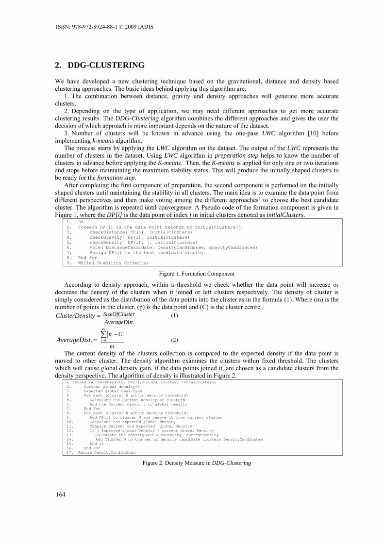
2. DDG-CLUSTERING

We have developed a new clustering technique based on the gravitational, distance and density based clustering approaches. The basic ideas behind applying this algorithm are:

1. The combination between distance, gravity and density approaches will generate more accurate clusters.

2. Depending on the type of application, we may need different approaches to get more accurate clustering results. The DDG-Clustering algorithm combines the different approaches and gives the user the decision of which approach is more important depends on the nature of the dataset.

3. Number of clusters will be known in advance using the one-pass LWC algorithm [10] before implementing k-means algorithm.

The process starts by applying the LWC algorithm on the dataset. The output of the LWC represents the number of clusters in the dataset. Using LWC algorithm in preparation step helps to know the number of clusters in advance before applying the K-means. Then, the K-means is applied for only one or two iterations and stops before maintaining the maximum stability status. This will produce the initially shaped clusters to be ready for the formation step.

After completing the first component of preparation, the second component is performed on the initially shaped clusters until maintaining the stability in all clusters. The main idea is to examine the data point from different perspectives and then make voting among the different approaches’ to choose the best candidate cluster. The algorithm is repeated until convergence. A Pseudo code of the formation component is given in Figure 1, where the DP[i] is the data point of index i in initial clusters denoted as initialClusters.

1. Do 2. Foreach DP(i) is the data Point belongs to initialClusters(j) 3. checkDistance( DP(i), initialClusters) 4. checkGravity( DP(i), initialClusters) 5. checkDensity( DP(i), j, initialClusters) 6. Vote( DistanceCandidate, DensityCandidates, gravityCandidates) 7. Assign DP(i) to the best candidate cluster 8. End for 9. While( Stability Criteria)

Figure 1. Formation Component

According to density approach, within a threshold we check whether the data point will increase or decrease the density of the clusters when it joined or left clusters respectively. The density of cluster is simply considered as the distribution of the data points into the cluster as in the formula (1). Where (m) is the number of points in the cluster, (p) is the data point and (C) is the cluster centre.

=sityClusterDen

.tAverageDisterSizeOfClus

(1)

=.tAverageDis

m

Cpm

ii∑

=

−0 (2)

The current density of the clusters collection is compared to the expected density if the data point is moved to other cluster. The density algorithm examines the clusters within fixed threshold. The clusters which will cause global density gain, if the data points joined it, are chosen as a candidate clusters from the density perspective. The algorithm of density is illustrated in Figure 2.

1. Procedure CheckDensity( DP[i],current cluster, IntialClusters) 2. Current global density=0 3. Expected global density=0 4. For each (Cluster N within density threshold) 5. Calculate the current density of clusterN 6. Add the Current densit y to global density 7. End For 8. For each (Cluster N within density threshold) 9. Add DP[i] to cluster N and remove it from current cluster 10. Calculate the Expected global density 11. Compare Current and Expected global density 12. If ( Expected global Density > current global Density) 13. Calculate the densityGain = ExDensity- currentDensity 14. Add Cluster N to the set of density candidate clusters DensityCandidates 15. End if 16. End For 17. Return DensityCandidates;

Figure 2. Density Measure in DDG-Clustering

ISBN: 978-972-8924-88-1 © 2009 IADIS

164

The second perspective is to examine the cluster according to its gravitational force. There exists a kind of force between any two objects in the universe and this force is called gravitation force [7]. According to Newton universal law of gravity, the strength of gravitation between two objects is in direct ratio to the product of the masses of the two objects, but in inverse ratio to the square of distance between them. The law can be described as follows:

221

rmmGFg = (3)

Where F is the gravitation force between two objects; G is the constant of universal gravitation; m1 is the mass of object 1; m2 the mass of object 2 and r the distance between the two objects.

Each cluster generates its own gravitational force created from its weight. The bigger the weight of the cluster the stronger the gravitational force produced from it. And therefore, the more points that cluster can attract. If the data point location is within the gravitational field of a cluster, then the data point will be attracted by this cluster’s gravitational force. Therefore, that cluster will be considered as a candidate cluster from the gravitational point of view. The gravitational threshold controls the size of the gravitational field surrounding the cluster. A pseudo code for the gravity measure is given in Figure 3.

1. Procedure CheckGravity( DP[i], intialClusters) 2. For each (Cluster N in the intialClusters and) 3. Calculate the distance between the centre of cluster N and DP[i] 4. Calculate the gravitational force between DP[i] and cluster N 5. If (gravitational force is within the gravitational threshold) 6. Add Cluster N to the set of gravity candidate clusters GravityCandidates 7. End If 8. End For 9. Return GravityCandidates;

Figure 3. Gravity Measure in DDG-Clustering

The data points are lastly checked from the distance based prospective. After Applying the density, gravity and distance examination, we get a set of candidate clusters from each approach. The voting system is used to decide which cluster is the best candidate to allocate the data point in. The pseudo code for the voting system is illustrated in Figure 4.

1. Procedure Vote( DistanceCandidate, DensityCandidates, gravityCandidates) 2. For each (Cluster N in the candidate clusters) 3. If( Cluster N is the DistanceCandidate and Cluster N is member in DensityCandidates and Cluster N is member in the GravityCandidates 4. Set Cluster N as the best candidate cluster 5. Else If( Cluster N is the DistanceCandidate and Cluster N is member in the DensityCandidates) 6. Calculate DensityGain as Cluster N DensityGain 7. For each (Cluster J in the DensityCandidates and Cluster J is member in the GravityCandidates) 8. Calculate DensityGain as Cluster J DensityGain. 9. End For 10. If( cluster J DensityGain> Cluster N Density Gain) 11. Set Cluster J as the best candidate Cluster 12. Else 13. Set Cluster N as the best candidate cluster. 14. End If 15. Else If (Cluster N in the DensityCandidates and Cluster N is member in the GravityCandidates) 16. Set Cluster N as the best candidate cluster. 17. Else If ( Cluster N is the DistanceCandidate and Cluster N is member in the GravityCandidates) 18. Set Cluster N as the best candidate cluster. 19. Else 20. Set DistanceCandidate as the best candidate cluster. 21. End If 22. End For 23. Return best candidate cluster;

Figure 4. Voting Among the Three Measures in DDG-Clustering

The formation component will be repeated till the number of points moved among clusters reduces and maintains certain percentage of accuracy. The relative importance of each approach is set by the user. In our experiments, we have assumed that all the measures have the same weight.

3. EVALUATION

To establish the practical efficiency of the proposed algorithm, we implemented it and tested its performance on a number of data sets. These included both synthetically generated data and data used in real applications. We generated data points in R2. The initial centres were chosen by taking a random sample. Then a Gaussian


165

distribution was then generated around each centre. We ran both K-means and DDG-Clustering algorithms. For each run, a new set of initial centre points and a new set of seed points were generated and both algorithms were run using the same data and initial centre points. The algorithms ran until convergence.

The results shown in Figure 5 illustrate how density and gravitational force could attract points effectively and allocate them to the right class. Although the points between the two clusters are assigned by the k-means to the closest cluster based on distance measure as in Figure 5(a), DDG-Clustering , as in Figure 5(b), assigned them to cluster 2 because it has a very strong gravitational force due to its weight that could attract these points toward it. On the other hand, the global density gain if these points assigned to the big cluster will be increased and therefore the points are assigned correctly to the big cluster.

K-means

0

50

100

150

200

250

300

350

400

450

0 100 200 300 400

Attribute1

Attrib

ute2

Cluster1

Cluster2

DGG-Clustering

0

50

100

150

200

250

300

350

400

450

0 50 100 150 200 250 300 350 400

Attribute1

Attrib

ute2

Cluster1

Cluster2

(a) K-means clustering output (b) DDG-Clustering clustering output

Figure 5. Comparing K-means and DDG-Clustering on Synthetic Dataset

Figure 6(a) explains how the initial seeds in k-means affected the clustering output, while DDG-Clustering could effectively detect the clusters correctly as in Figure 6(b).

K-means

0

50

100

150

200

250

300

350

0 100 200 300 400 500

Attribute1

Attr

ibut

e2

Cluster1Cluster2

DDG-Clustering

0

50

100

150

200

250

300

350

0 50 100 150 200 250 300 350 400 450

Attribute1

Attr

ibut

e2

Cluster1Cluster2

(a) K-means clustering output (b) DDG-Clustering clustering output

Figure 6. Comparing K-means and DDG-Clustering on Synthetic Dataset

Two well known real datasets from were selected for the experiments: glass and vehicle datasets are used for testing the accuracy of the proposed algorithm. Both datasets are from the UCI machine learning repository, which are available from the web site: http://www.ics.uci.edu/~mlearn/databases/. Main characteristics of these data sets are depicted in Table 1, including number of data samples, number of features (attributes) and number of data classes. Figure 7 shows the stability and fast convergence of DDG-Clustering when compared with K-means.

Table 1. Real Datasets Characteristics

Data Set name No. of samples No. of attributes No. of classes Glass 214 9 7 Vehicle 846 18 4

We applied DDG-Clustering on both vehicle and glasses datasets for 10 times and compared it with K-means. Both algorithms applied on the same seeds, while a new set of seed points was generated for each run. The results showed that DDG-Clustering attain higher accuracy in terms of number of points assigned correctly to clusters compared to K-means. When the number of clusters increases as in glasses dataset, DDG-Clustering algorithm operates more effectively as shown in Figure 8.

ISBN: 978-972-8924-88-1 © 2009 IADIS

166

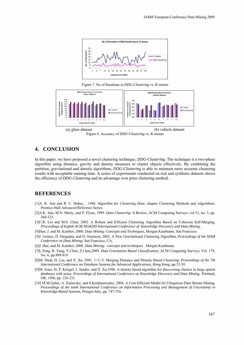
No. of iterations in DDG-Clustering vs. K-means

05

101520253035

1 4 7 10 13 16 19 22 25 28 31 34 37 40

experiment index

No.

of i

tera

tions

K-means

DDG-Clustering

Figure 7. No of Iterations in DDG-Clustering vs. K-means

DDG-Clustering vs. K-means Glass dataset

020406080

100120140160

1 2 3 4 5 6 7 8 9 10

experiment index

num

ber o

f cor

rect

ly

assi

gned

poi

nts

K-means

DDG-Clustering

DDG-Clustering vs.K-meansVehicle dataset

300

320

340

360

380

400

1 2 3 4 5 6 7 8 9 10

experiment index

num

ber o

f cor

rect

ly

assi

gned

poi

nts

K-means

DDG-Clustering

(a) glass dataset (b) vehicle dataset

Figure 8. Accuracy of DDG-Clustering vs. K-means

4. CONCLUSION

In this paper, we have proposed a novel clustering technique, DDG-Clustering. The technique is a two-phase algorithm using distance, gravity and density measures to cluster objects effectively. By combining the partition, gravitational and density algorithms, DDG-Clustering is able to maintain more accurate clustering results with acceptable running time. A series of experiments conducted on real and synthetic datasets shows the efficiency of DDG-Clustering and its advantage over prior clustering method.

REFERENCES

[1]A. K. Jain and R. C. Dubes, , 1988. Algorithm for Clustering Data, chapter Clustering Methods and Algorithms. Prentice-Hall Advanced Reference Series.

[2]A.K. Jain, M.N. Murty, and P. Flynn, 1999. Data Clustering: A Review, ACM Computing Surveys, vol.31, no. 3, pp. 264-323.

[3]C.R. Lin and M.S. Chen, 2002. A Robust and Efficient Clustering Algorithm Based on Cohesion Self-Merging, Proceedings of Eighth ACM SIGKDD International Conference of Knowledge Discovery and Data Mining.

[4]Han, J. and M. Kamber, 2000. Data Mining: Concepts and Techniques, Morgan Kaufmann, San Francisco. [5]J. Gomez, D. Dasgupta, and O. Nasraoui, 2003. A New Gravitational Clustering Algorithm, Proceedings of the SIAM

Conference on Data Mining, San Francisco, CA. [6]J. Han ,and M. Kamber, 2000. Data Mining: concepts and techniques . Morgan Kaufmann. [7]L.Peng, B. Yang, Y.Chen, Z.Chen,2009. Data Gravitation Based Classification, ACM Computing Surveys, Vol. 179,

No. 6, pp 809-819. [8]M. Dash, H. Liu, and X. Xu, 2001. 1+1>2: Merging Distance and Density Based Clustering. Proceedings of the 7th

International Conference on Database Systems for Advanced Applications, Hong Kong, pp.32-39. [9]M. Ester, H. P. Kriegel, J. Sander, and X. Xu,1996. A density-based algorithm for discovering clusters in large spatial

databases with noise. Proceedings of International Conference on Knowledge Discovery and Data Mining. Portland, OR, 1996, pp. 226-231.

[10] M.M.Gaber, A. Zaslavsky, and S.Krishnaswamy, 2004. A Cost-Efficient Model for Ubiquitous Data Stream Mining, Proceedings of the tenth International Conference on Information Processing and Management of Uncertainty in Knowledge-Based Systems, Perugia Italy, pp. 747-754.


167

Posters

WIEBMAT, A NEW INFORMATION EXTRACTION SYSTEMEN

El ouerkhaoui Asmaa, Driss Aboutajdine University of Mohamed V Agdal

Faculty of science, 3 Ibn Batouta Avenue PO BOX 1040, Rabat, Morocco

Doukkali aziz ENSIAS

PO BOX 6541, Medinat Al Irfane, Rabat, Morocco

ABSTRACT

Being aware of the amount of information containing in Internet, many researchers are now turning their attention to a relatively new task orientation known as IE (information extraction). Information extraction systems are predicated on an I/O orientation that makes it possible to conduct formal evaluations and meaningful cross-system comparisons. This paper introduces a new IE system: WiebMat which describe a specific system developed at the University of Mohamed V. Information Extraction Systems provides tools for building high-performance, multilingual, adaptive, and platform-independent natural language processing applications.

KEYWORDS

IE(Information extraction), Wrapper Induction systems, structured and semi-structured document, unsupervised systems XML.

1. INTRODUCTION

Internet is a much consulted information source and a very wealthy one. Many tools are used to search this information as search engines where user’s job is limited to enter one or more key words relative to its research. This tool has been a real revolution, but the amount of information in Internet is not totally exploited, the number of search engines dedicated to a specific area is limited. Thus, many researchers focused on this problem and they create a new research area which is IE (Information Extraction) from the Web. Many approaches have been developed and many WI (Wrapper Induction) or IE systems have been proposed.

2. WIEBMAT, A NEW APPROACH FOR IE FROM WEB PAGES

WIEbMat stands for Wrapper Induction Environment based on Matrixes, a wrapper induction [1][2][3] is a technique for automatically learning wrapper. A lot of IE system which lies on an induction environment has been proposed in the literature. We have also implemented another approach called Gene/Clone [4][5][6][7][8][9][10]. WIEbMat stands on matrixes to extract relevant data, thus we build an initial matrix which contains relevant and noisy data, by means of some calculated parameters we delete each row which contains at least one null element and we obtained at the end of the process a final matrix which contains only relevant data. We obtained very satisfying results by using this technique (almost 96%). The real problem which reduce this rates is the process of XMLisation (transforming a web pages coded in HTML into a XML) that’s why we create a new parameter which calculates the capacity of the system to XMLisate a web page before performing information extraction, thus we prove that the WIEbMat techniques is not responsible of extracting sometimes noisy data.


171

We implement this approach to create a Meta Search Engine called BERG, it uses in its back office as many search engines that we configure in its back office.

Figure 1. The main graphical interface of BERG

Once one or several keywords are entered in the text box shown in the figure 1 we obtained as much as results found using the search engines configured in the back office.

Figure 2. A response Web page of BERG

To configure a search engine in the BERG’s back office we have to enter first of all the information shown in the third figure which are the source URL (Unified resource Locator) using at least two key word, and the URL of the second response web pages. Add to this we enter the name of the search engine to identify it and the number of results found in one single web page.

Figure 3. First graphical interface of BERG back office’s

After that, we are redirected to the second graphical interface where we enter two example instances as shown in the figure four. This pattern may then be used to retrieve other instances.

ISBN: 978-972-8924-88-1 © 2009 IADIS

172

Figure 4. Second graphical interface of BERG back office’s

As shown in this figure, we use a frame which contains a view of the first response web page obtained to take the pattern from it.

3. CONCLUSION

The solution that we proposed for the construction of an adapter for Web data sources leans on a set of example’s instances of a relation to be extracted from these sources. The contexts of these instances are then extracted of a set of pages of the source. This method has several advantages with regard to the previous methods; it allows users to express simply their need of information as a set of instances of a relation to be extracted. The number of example’s instances to be given is often reduced: generally two or three instances for each source are enough.

REFERENCES

Journal Kushmerick, N. , Weld, D. ,and Doorenbos, R. , Wrapper induction for information extraction. Proceeding of the 5th

International conference on artificial intelligence (IJCAI), pp.729-735, 1992 Kushmerick, N. , Weld, D. ,and Doorenbos, R. , Wrapper induction for information extraction. Proceeding of the 5th

International conference on artificial intelligence (IJCAI), pp.729-735, 1992 Conference paper or contributed volume Habegger, B., Extraction d’information à partir du Web, thèse pour obtenir le grade de docteur de l’Université de Nantes,

2004. El Habib BEN LAHMER, Abd Elaziz SDIGUI DOUKKALI, Mohamed OUMSIS. La Meta recherché générique: vers la

génération des Meta moteurs de recherche. CopStic’03 Rabat, Maroc. El Habib BEN LAHMER, Abd Elaziz SDIGUI DOUKKALI, Mohamed OUMSIS. Towards an automatic extraction of

data from half-structured documents. In ISCCSP2006. El Habib BEN LAHMER, Abd Elaziz SDIGUI DOUKKALI, Mohamed OUMSIS, 2004, WBERG, un Meta annuaire

WAP, in isivc’04 Brest France. El Habib BEN LAHMER, Abd Elaziz SDIGUI DOUKKALI, ElOuerkhaoui Asmaa. (2006). A solution for data

extraction by a new approach: The method of Gene/Clone. ICT4M: Kuala Lumpur, Malaysia. El Habib BEN LAHMER, Abd Elaziz SDIGUI DOUKKALI, ElOuerkhaoui Asmaa. (2006). BERG 2.2: a Meta search

engine for on-line directories. ISCIT’06, Bangkok, Thailand. El Habib BEN LAHMER, Abd Elaziz SDIGUI DOUKKALI, ElOuerkhaoui Asmaa. (2006). A new solution for data

extraction: Gene/Clone method. IJCSNS volume 6. ElOuerkhaoui Asmaa, Abd Elaziz SDIGUI DOUKKALI. (2006). Comment render le contenu informationnel sur Internet

intelligible. WOTIC’07, Rabat, Maroc.


173

CLUSTER OF REUTERS 21578 COLLECTIONS USING GENETIC ALGORITHMS AND NZIPF METHOD

José Luis Castillo Sequera, José R. Fernández del Castillo, León González Sotos Department of Computer Science, University of Alcalá, Madrid, Spain

ABSTRACT

In this paper, we discuss a feature reduction technique and their application to document clustering, showing that feature reduction improves efficiency as well as accuracy. We select the terms starting from the Goffman point, selecting an area of suitable transition making use for it of the Zipf law (our method is called NZIPF). Finally, we demonstrate experimentally that the transition zone that provides better results is taking 40 terms starting from the Goffman point for a cluster of documents with a genetic algorithm non-supervised. The experiments are carried out with the collection Reuters 21578 and the results are grouped by new genetic operators designed to find the affinity and similarity of the documents without having prior knowledge of other characteristics.

KEYWORDS

Clustering, Information Management, Information Search and Retrieval, Data Mining.

1. INTRODUCTION

Document clustering has attracted much interest in the recent decades [1] [3][4][6], and much is known about the importance of feature reduction in general [1], but little has been done so far to facilitate reduction for document clustering of query results, hence, we carry out a system that reduces the dimensionality, and we validate it experimentally with a genetic algorithm with news operators of clustering. We select the terms of document starting from the Goffman point [5], selecting an area of suitable transition making use for it of the Zipf law [7]. First, a list of stop-words and stemmer was used to reduce words of the language.

GA is an iterative procedure which maintains a constant size population of feasible solutions, during each iteration step, called a generation, the fitness of current population are evaluated, and population are selected based on the fitness values. The chromosomes are selected for reproduction under the action of crossover and mutation to form new population. We propose a system of clustering of documents through a GA with new operators of crossover and mutation, we implement the GA in the collection Reuters 21578 and we compare the effects of different values of mutation rates. One the main contributions is also the form like the documents are represented, using a method that selects the terms of documents starting from the Goffman point, selecting an area of suitable transition making use for it of the Zipf law, our method is called NZIPF. In GA, the aptitude of the individuals this based on the measures of the euclidean distance and coefficient of correlation of Pearson, that allows it to find the most similar documents.

2. IMPORTANCE OF ZIPF’s LAW AND USING THE METHOD NZIPF

This law treats the frequency of the use of the words in any language. It proposes that inside a communication process, they usually use most often some terms, because the authors usually avoid the search of more vocabulary to express their ideas [7]. Zipf establishes that if we order the words of a text for falling order of occurrence, the frequency of the word that occupies the position "r" will come given by a distribution frequency-range: KFR =* . This expression indicates that the product of the frequency of a word for its range is constant. Where: R = it is the order of the word in the list, F = it is the frequency of that word, and K = it is the constant for the text. Another law of Zipf that is developed next: If we call: I1 to the

ISBN: 978-972-8924-88-1 © 2009 IADIS

174

word count frequently 1, In to the word count frequently "n" Verified that: ( )2

11 +⋅=

nnII

n

. Leaving of

these laws, Goffman established a procedure to eliminate the non outstanding terms of the documental base [5]. According to Goffman, the articles, conjunctions, etc are the words of higher frequency and the words of very low frequency are the strangest words that denote the style or vocabulary. The transition zone should be in the area in that In, this is, the word count of frequency near at 1, then with In=1, we obtain:

.2

811 1In

⋅++−= Therefore, finding that "n" (Point of Goffman), they would serve us as terms

indexers (figure 1). The transition area has the terms indexes of the documental base (figure 2). This is all the words of frequency "n", and those of frequencies n-1, n-2,... and n+1, n+2... until having a number of terms appropriate. In our experiments we make vary the number of terms from < n-K, n+K > until being able to obtain the best vectors that allow to obtain a better representation of the documental base (NZIPF).

Once we have obtained all the terms with discriminatory bigger power, the process consists on the

construction of vectors with the size of the terms. A document "gave" it will be identified by means of a collection of terms Ti1, Ti2.....Tit where Tij represents the weight of the term j (table 1). The experimental tests were carried with more than 25% of collections Reuters. The objective was to obtain a transition area that provides bigger number of successes starting from the point of Goffman. We show that it is necessary to select only 40 lemmatisers terms from the point of Goffman to reduce the dimensionality (figure 3).

0

1

2

3

4

Number of successes

on 4 groups

taken at random

10 20 30 40 50 60 70Number of terms lematizados in the transition area

Evolution of the number of successes w ith the method Nzipf in 4 groups taken at random for the 6 pirmeras distributions of the collection Reuters 21578

according to the transition area to evaluate

Distribution 0 Reuters Distribution 1 Reuters Distribution 2 Reuters

Distribution 3 Reuters Distribution 4 Reuters Distribution 5 Reuters

Figure 3. Evolution of Successes (NZIPF with 4 groups)

Table 1. Vectorial representation of the documental base

.Documents T1 T2 T3 ……. Tt

Docum. 1 T11 T12 T13 …… T1t

Docum. 2 T21 T22 T23 …… T2t

Docum. 3 T31 T32 T33 …… T3t

………. ---- … ….. …… ….

Docum. N Tn1 Tn2 Tn3 ……. Tnt

Table 2. Measures of the Function

Distance Euclidean ∑ −

=

=t

kij xxd jkik

1

2)(

Coefficient correlation of Pearson (Similarity) ⎟

⎟⎟⎟

⎠

⎞

⎜⎜⎜⎜

⎝

⎛−

⎟⎟⎟⎟

⎠

⎞

⎜⎜⎜⎜

⎝

⎛−

= ∑= x

xxxxx

j

jn

i i

i jin

rσσ

_

1

_

1

Fitness Global

Min (α Distance(Documents i) + Β (1/ Similarity(Documents i )) )

Figure 1. Point of Goggman Figure 2. Area of Transition of Goggman


175

3. EXPERIMENTATION OF GENETIC ALGORITHM

Clustering purpose is to divide a given group of documents in a number of groups in order that the objects in a particular cluster would be similar among the documents. The formal procedures use an optimization criterion. We apply the distance Euclidean and the Coefficient of Pearson simultaneously to evaluate the fitness of GA with new crossing operators and mutation designed for the problem. We use the terms have been obtained applying a processing of documents with the NZIPF method. Then we place in “preorder” all the documents in a tree structure. We generate the individual in a random way with a population of 50 or 200 individuals, the length of the chromosome depends on the number of documents to group. After that the genetic operators generate a new population (figure 4).

We use two measures of fitness (distance and similarity) attempt on one hand to maximize the similarity of the documents and by another to minimize the distances among them.

Table 3. Parameters of Genetic Algorithm

Population Size

50 few documents

200 Many documents

Mutation rate (Tm)

0.70, 0.75, 0.80, 0.85, 0.9,0.95

Tournament Size

2 Crossover rate (Tc)

0.7

Number of Generations

1000 Number of test by sample

1, 2, 3, 4, 5

Number of tokens terms

40 Adjustment α

Tm * Tc

Adjustment β

1-α

Figure 4. Initial Population of Individuals The 2 types of measures of fitness are show in table 2. Where: α: it will be the parameter that adjustment

the similarity and β: it will be the parameter that adjustment the distance. The GA was processed with the parameters of table 3 taking samples documents from the collections at random (up to 3 different samples of 80 documents that we call “many documents”). We always try to maximize the number of successes of GA.

4. CONCLUSIONS AND FURTHER WORK In this paper we show that it is necessary to select only 40 lemmatisers terms of the transition area from the point of Goffman to reduce the dimensionality of the vector documentary using our method called NZIPF to implement it in a grouping of documents with a genetic algorithm. The maximum number of hits of GA is when using the rate of mutation of 0,85. The results show that the grouping obtained with these terms is robust because the results are very similar to the true of the collections Reuters.

REFERENCES Baeza-Yates R, Ribeiro-Neto B. ”Modern Information Retrieval” Addison Wesley 1999. Cordon, Herrera, Hoffman & Magdalena “Genetic Fuzzy System”, Word Scientific 2001. Marcus A. Malov. “Machine Learning and Data Mining for Computing Security” Springer 2006 Olson David and Dursun Delen. “Advanced Data Mining Techniques”, Springer 2008. Pao M.L, 1976 “Automatic indexing based on Goffman transition of word occurrences”.American Society 1980. Salton G. “Automatic Text Processing by Computer”. Addison-Wesley, 1989. Zipf GK. “Human Behavior and the Principle of Least Effort”. Addison Wesley, 1949.

Documentary Collections Method Preprocessing

NZIPF Vectors (Lexemes) Characteristics

Creation of the Initial Population

F

f

Individual 1 Individual N=50

F: Fitness global f: Fitness local

f

f D5

D6

f D3

D1 D2

F

f f

f D4

D3 D5

f D1

D6 D2

Chromosome 50: 00035400621

Chromosome 1: 00506400123

D4

ISBN: 978-972-8924-88-1 © 2009 IADIS

176

I-SOAS DATA REPOSITORY FOR ADVANCED PRODUCT DATA MANAGEMENT

Zeeshan Ahmed Vienna University of Technology

Getreidemarkt 9/307 1060 Wien Austria

ABSTRACT

In this poster paper I shortly discuss an intelligent semantic based approach, proposed as the solution towards the problems of static and unintelligent search, platform independent system and successful PDM system implementation in the field of Product Data Management (PDM). Moreover I discuss database management system designs especially designed for the Product Data Management based software application.

KEYWORDS

I-SOAS, PDM, Repository.

1. I-SOAS REPOSITORY

Product Data Management (PDM) is a digital electronic way of maintaining organizational data to maintain and improve the quality of products and followed processes. Where PDM based products are heavily benefiting industry there PDM community is also facing some serious unresolved issues .i.e., successful secure platform independent PDM system implementation, PDM system deployment and reinstallation, static and unfriendly machine interface, unintelligent search and scalable standardized framework. Targeting above mentioned PDM based problem oriented issues I have proposed an approach called Intelligent Semantic Oriented Search (I-SOAS) (A. Zeeshan, 2008). I-SOAS implementation architecture is consist of four main modules .i.e., I-SOAS Graphical Interface, I-SOAS Data Repository, I-SOAS Knowledge Base, I-SOAS Processing Modelling and three communication layers .i.e., Process Presentation Layer (PPL), Process Database Layer (PDL), and Process Knowledge Layer (PKL). In this research I am not going in details of any other component of I-SOAS except I-SOAS Data Repository. I-SOAS Data Repository module is to store, extract, transform, load and manage organizational technical and managerial data. Moreover I-SOAS Data Repository is supposed to work like other Data Warehouses by providing several options to produce common data model for all data of interest easier to report and analyze information, prior loading data, security and retrieval of data without slowing down operational systems.

The I-SOAS Database must be designed keeping two major record keeping requirements .i.e., Organizational Data and System Data in mind. The designed Organizational database must be capable of storing and managing organizational technical and non technical data divide into three sub major categories User Data, Project Data and Product Data. The designed entity relationship diagram of I-SOAS Database Organizational Data is consists of 5 main relations .i.e., Organization, Person, Staff, Project, Product and 17 supportive relations .i.e., Name, Contacts, Contacts_Web, Contact_Telephone, Contact_City, City_Country, City_State, Start_End_Date, Project_Team, Meeting, Activity, Staff_Meeting, Document, Type, Staff_Document, Organisation_Document, Project_Document designed and connected to store and manage organizational data, employee’s (user) personal data, project data and product data (See Fig 1).


177

Figure 1. Organizational Data Design (A. Zeeshan 2009)

The designed System database must be capable of storing and managing System Data containing the information about user inputs, system output, actions, reactions, input processing, The designed entity relationship diagram of I-SOAS Database System Data Design is consists of three relations .i.e., Login, SystemInput and SystemOutput (See Fig 2).

Figure 2. Organizational Data Design (A. Zeeshan 2009)

As this research paper is about an ongoing in process research project, right now I am developing I-SOAS Data Repository as a real time software application by implementing above discussed designs.

REFERENCES

A. Zeeshan, 2009. PDM based I-SOAS Data Warehouse Design, In the proceedings of FIFTH International Conference on Statistical Sciences, Mathematics, Statistics and Applications, Organized by NCBA&E, COMSATS and ISOSS, Paper ID 125, January 23-25, 2009, Gujrat Pakistan 2009

A. Zeeshan, D. Gerhard, 2008. Intelligent Graphical User Interface, Information Processing and Data Management based Solution towards Intelligent Data Manipulation and Representation, In the proceedings of 4th Virtual Conference Network of Excellence on Innovative Production Machines and Systems, IPROMS 2008, 1-15 July, Cardiff England 2008

ISBN: 978-972-8924-88-1 © 2009 IADIS

178

DATA PREPROCESSING DEPENDENCY FOR WEB USAGE MINING BASED ON SEQUENCE RULE ANALYSIS

Michal Munk, Jozef Kapusta, Peter Švec Department of Informatics, Constantine the Philosopher University in Nitra

Tr. A. Hlinku 1, 949 74 Nitra, Slovakia

ABSTRACT

Systematic analysis of a portal with modifying content on regular basis represents a very important phase of its development. Data for the analysis is provided by a web server log file. However, the analysis of the file log is time consuming and so is data preprocessing from the file. Purging the data by excluding the search engines visits and perhaps also visitors coming from NAT or proxy devices is very important. We also detect user sessions by defining time slots. In this paper we are dealing with a problem which data preprocessing steps are required and define which of these steps can be integrated and automated. We made an experiment and compared results of sequence rule analysis of four files preprocessed in different levels. We tracked count of web accesses, count of costumers’ sequences, count of frequented sequences, and proportion of discovered rules and values of confidence of discovered rules between the files. Experiment results suggest that including the session time slots is very important for sequence rule analysis despite excluding search engines robots.

KEYWORDS

Sequence rule analysis, web usage mining, data preprocessing.

1. INTRODUCTION

University Web portal, as one type of a web portal, is an information system, where university employees, students and others seek information related not only to their study but also tasks and other opportunities the university offers. The order of menu items and the content of each item were created based on portal analysis and information arrangement, which the university provides. As it may not be optimal we optimize it by application of sequence rule analysis to web logs (Munk, 2009).

Data for a web portal analysis with anonymous visitors is gathered from a web server log file. The data is usually represented in a standard format e.g.: Common Log Format or Extended Log Format. We used the Common Log Format that stores information about IP address, date and time, http method, URL and agent information. Access to the portal is anonymous so a problem appears with identification of a single user or a single visit in case we do not use session IDs or cookies. Preprocessing of web logs is usually complex and time consuming. It comprises four different tasks: data clearing, identification of users’ sessions, obtained information about page content and structure and data formatting (Bamshad, 2000).

Data clearing and session identification consist of removing all data tracked in weblogs unnecessary for mining purposes, e.g. requests for images, styles or scripts or any other file that might be integrated on the website. Elimination of robots is not very difficult either. Today’s robots, or more precisely most of them, identify themselves through the user-agent field in web logs. If users’ network uses NAT we can only see one IP address in web logs despite the fact that there are many users accessing our website. We must decide if we want to eliminate NAT and proxy users from analysis. If so, we must identify user’s sessions. In this case we can as well identify users that share one PC, e.g. in a library or school. The session presents a time limited series of clicks. This time limitation is estimated. Bettina and Myra (2000) used 30-minute time slot, we used Google Analytics to estimate time slot to 10 minutes.


179

2. EXPERIMENT

The experiment was performed in five steps: 1. Data acquisition – defining variables into a web log (IP address, date and time, URL, user-agent). 2. Designing the data matrix – based on the web log data (access) and site map (content). 3. Four levels for data clearing and preparation (Table 1). 4. Data analysis – detection of behavioral patterns of users’ behavior. 5. Comparison – of analysis results on different levels of data preparation (proportion of discovered

rules, values of support characteristics of discovered rules within files, values of confidence of discovered rules within files).

A file with raw data (File 1) contains almost 40.000 lines (Table 1) and represents accesses to the portal in a period of one week. There are almost 11% of robots accesses and more than 9% of NAT/proxy accesses.

Table 1. Number of Accesses, Identified and Frequented Sequences in Particular Files

Count of web Accesses

Count of costumer's sequences

Count of frequented sequences

(File 1): raw data/ log file without useless data 39688 4506 90 (File 2): data without robots 35374 4454 91

(File 3): data without robots and without NAT/proxy devices 31761 4242 87

(File 4): data without robots and with session identification 35374 8875 37

We monitored access to university portal in a period of one week. Results of the analysis represent sequence rules (Table 2.), obtained from frequented sequences that fulfill minimal support (s = 0.03 in our case). Frequented sequences were obtained from identified sequences, i.e. visits of UKF portal in one week period.

Table 2. Discovered Sequence Rules in Particular Files

Sequence rules (File 1) (File 2) (File 3) (File 4) Body ==> Head s(1) c(1) s(2) c(2) s(3) c(3) s(4) c(4)

( a180 ) ==> ( a180 ), ( a180 ) 4.28 37.92 4.33 38.45 4.13 37.55

…

…

…

…

…

…

…

…

…

…

…

( a49 ) ==> ( a180 ), ( a178 ) 3.01 20.68 Count of derived sequence rules 75 75 78 78 72 72 13 13

Percent of derived sequence rules 96.2 96.2 100.0 100.0 92.3 92.3 16.7 16.7 There is a high level of conformity (Table 2) between the results of sequence analysis regarding the ratio

of rules discovered in the first three files. More specifically, most of the rules, in particular 78 rules, were derived from files excluding robots (File 2). Other 75 rules were derived from raw data (File 1) and last 72 rules were derived from a file excluding robots and NAT/proxy devices. In File 1 and File 3 the ratio of discovered rules includes over 90% rules more than File 2. The difference in discovered rules count between the first three files is minimal.

We assumed that excluding robots and NAT/proxy devices from the log will have a great impact on the results. Rules found in a log excluding robots (File 2) were derived also in raw log (File 1). The difference was in just three new rules derived in the log excluding robots (File 2). We discovered less than 6 rules in the log excluding NAT/proxy (File 3) than in the log excluding robots (File 2). The remaining rules were identical with rules derived in the raw log (File 1) and log excluding robots (File 2).

On the other hand, there is a great difference in a number of discovered rules between the log with sessions (File 4) and the remaining logs. The ratio of discovered rule is less than 20% of discovered rules in log excluding robots (File 2). Though this ratio is the least significant there is no illogical rule (Table 2), for example:

( a180 ) ==> ( a180 ), ( a180 ), support = 4.28, confidence = 37.92 We can interpret this rule as follows: If a user visits the Telephone Directory there is a probability of 38%

that he will visit the Telephone Directory and the Telephone Directory. By creating time slots to identify users’ sessions we do not only exclude NAT/proxy to our analysis, but

we also eliminate the problem of multiple users sharing one computer. Doing this, we reduce inconsequent

ISBN: 978-972-8924-88-1 © 2009 IADIS

180

sequences. Sharing one computer is typical for example for classrooms or libraries. Results of the analysis show that no illogical rules were found only in File 4.

We can also find a high level of conformity in the sequence rule analysis when it comes to support characteristics values of discovered rules in particular files. The Kendall coefficient of concordance represents conformity rate in support of discovered rules among particular files. The Kendall coefficient value is 0.9716. If the value is equal 1 we find a perfect match. If the value is equal 0 we find a mismatch (Hendl, 2004).

In the correlation matrix (Table 3) we can see, that the highest value of conformity/dependency in support can be found in rules discovered in raw log (File 1), log excluding robots (File 2) and log excluding robots and NAT/proxy (File 3). Not very distinct, but quite a significant difference (p < 0.05), is between log with sessions (File 4) and other log files.

Table 3. Kendall Tau Correlations for Support

s(1) s(2) s(3) s(4) s(1) 1.000 0.998 0.948 0.795s(2) 0.998 1.000 0.950 0.795s(3) 0.948 0.950 1.000 0.795s(4) 0.795 0.795 0.795 1.000

Table 4. Kendall Tau Correlations for Confidence

c(1) c(2) c(3) c(4) c(1) 1.000 0.995 0.974 0.744c(2) 0.995 1.000 0.973 0.769c(3) 0.974 0.973 1.000 0.718c(4) 0.744 0.769 0.718 1.000

There is a relatively high conformity regarding the confidence characteristic of discovered rules in particular files. Kendall coefficient of concordance represents level of conformity in confidence of discovered rules. The value of coefficient is 0.6064, whereas the value of 1 represents perfect match and value of 0 represents mismatch (Hendl, 2004).

In the correlation matrix (Table 4) we can see that the highest value of conformity/dependency in confidence was found in the raw log (File 1), log excluding robots (File 2) and log excluding robots and NAT/proxy (File 3). Not very distinct, but quite a significant difference (p < 0.05), is between log with sessions (File 4) and other log files.

3. CONCLUSIONS AND FUTURE WORK

Our experiment reveals a few important facts. It is remarkable that most rules were discovered after clearing robots from the data (browsing the site recursively), however with no significant effect for frequented sequences discovered by sequence rule analysis. Similar effect was achieved by excluding NAT/proxy devices. In contrary, the identification of sessions by time slots presents the most important step in the data processing. The session identification process can be improved by detecting different agents (browser) from the same IP, by detecting the cache using and by estimation of time slot which may differ from portal to portal and different time periods (Munk, 2008). Each data preprocessing step consisted of several applications. Our aim is to integrate this application into one general application.

REFERENCES Bamshad, M., Robert, C. et al, 2000. Automatic personalization based on Web usage mining. In Commun. ACM, Vol. 43,

No. 8, pp 142-151. Bettina, B. and Myra, S., 2000. Analysis of navigation behaviour in web sites integrating multiple information systems.

In The VLDB Journal, Vol. 9, No. 1, pp 56-75. Hendl, J., 2004. Prehled statistickych metod zpracovani dat: Analyza a metaanalyza dat. Portal, Praha, CR. Munk, M., 2008. Web optimization base on sequence rules. In Forum Statisticum Slovacum, Vol. 4, No. 7, pp 80-85. Munk, M., 2009. Web usage mining-methods and applications. In Forum Statisticum Slovacum, Vol. 5, No. 1, pp 65-72.


181

GEOGRAPHIC DATA MINING WITH GRR

Lubomír Popelínský1 Knowledge Discovery Lab

Faculty of Informatics, Masaryk University Brno Botanická 68a, 60200 Brno, Czech Republic

ABSTRACT

In this paper we describe new version of GRR, a tool for mining in geographical information systems which is a part of CriMi framework for mining in crisis management data. We aimed at building a platform–independent tool for mining in GIS, easily available for users, especially for non-expert in data mining.

KEYWORDS

Data mining, geographic data, crisis management.

1. GEOGRAPHIC DATA MINING AND CriMi

The tasks when mining geographic data are similar to those in general data mining, namely understanding data, discovering hidden relationship in data – e.g. classification, clustering and subgroup discovery – (re)organizing geographic databases etc. Starting from 90’th, many systems for spatial data mining have been developed that employ various learning techniques, maybe the most influential between them GeoMiner (Han et al. 1997). GeoMiner was able to find different kinds of rules, including characteristic rules, comparison rules, and association rules. The SPIN! project aimed at building a geographic data mining system for mining in official data. INGENS [15] aims at map interpretation. Inductive queries are expressed in SDMOQL, the extension of object–oriented query language OQL. Geographic data need to be stored in ObjectStore DBMS. ComonGIS enable spatial intelligent data visualization in interactive thematic maps and also offer tools for interaction with a map. All these systems offer mining capabilities with no need of programming. However, the menu of learning algorithms used to be limited. Moreover, an extension of these tools can be difficult, or even impossible without deep understanding of a particular system. competencies.

Here we introduce a new version of GRR, a system for mining in geographic information systems which is as a part of CriMi framework. The aim of this framework (Večeřa et al.) is to support civil crisis management plans in various areas based on machine learning (learning from one relation, ML) and multi-relational data mining (MRDM). This involves spatio-temporal data preprocessing, implementation of appropriate rules for learning systems, and eventually integration of the whole process into local civil crisis management planning. To the best of our knowledge, there is no comprehensive work on spatio-temporal multi-relational data mining for civil crisis management. The outcome of this work will be a proof of concept on floods data that could be used in local civil crisis management planning.

2. GRR

GRR is a general tool for mining in a geographic information system (GIS). We aimed at building a platform–independent tool for mining in GIS, easily available for users, especially for non-expert in data mining. GRR employs different learning and statistical methods and can be easily extended. GRR offers tools from R packages and Weka as well as multi-relational learning (MRDM, inductive logic programming, ILP)

1 The author has been partially supported by Faculty of Informatics, Masaryk University Brno and by the grant MSMT 0021622418 Dynamic geovisualization in crisis management.

ISBN: 978-972-8924-88-1 © 2009 IADIS

182

algorithms. GRR is composed of a graphical user interface, a module for communication with R system and Weka

classes and for communication with the geographic information system GRASS. The previous version of GRR has been described in (Buk and Kuba 2001).

GRR is a tool for mining in GRASS (http://grass.itc.it/) geographic information system. GRASS (Geographical Resources Analysis Support System) is a geographical information system is open-source free software released under GNU General Public License. The R system (http://www.r-project.org) provides wide range of statistical methods and machine learning algorithms, as well as visualization tools.

In the current version, GRR offers main pre–processing methods, analytic tools from R and also two multirelational data mining tools – Aleph and RAP – that enable to learn from vector data. Newly the tools from Weka packages has been added antd the interface with GIS GRASS has been adapted.

3. EXPERIMENTS

Here we now demonstrate an incorporation of Weka into GRR. The Weka machine learning toolbox which is implemented in Java and available under GNU license is being developed at University of Waikato, New Zealand (Witten and Frank 2005). It contains a wide repertoire of pre-processing and learning algorithms as well as tools for data visualization. The current version can process both attribute-value data and multi-instance data. Initialization script has been extended with a path to Weka directory with weka.jar . The main modification concerned a Perl script for GUI which has been extended with a new menu and an interface between Weka and internal format of learning data.A user can choose layers of data and then a classifier – its name, parameters, a way of validation of a result, and verbosity. After learning a classifier and classifying test data a user may ask the system to build a new layer from the result of classification.

Figure 1. Classification of Landcover: Original Data, the Previous Version of GRR, a New Version of GRR (Naïve Bayes

and a Decision Tree)

For demonstration of GRR capabilities we used raster data covering north–west part of Leicestershire, England that are as a part of GRAS distribution. The data cover an area of 12km by 12km, including two towns, Loughborough a Shepshed, with dense network of roads of different categories, railroads and Soar river. The northern and the eastern parts are rather flat, the rest is covered by highlands. The data consists of the following layers: crash – highway accidents; contours – contour lines; image – monochrome satellite image; landcov – exploitation of each pixel (e.g. industrial, urban, forest, bush, water etc.); plant – cleaner of water; popln – settled or non-settled ; rail – railways; roads – roads with their classification; segment – the polluted segment of Soar river; source – the source of pollution; spillage – the degree of pollution risk; topo –


183

altitude; urban – important urban regions water – rivers and lakes. The original landscape layer and results for the previous version of GRR and for various newly added learning algorithms are on Pic.1.

4. CONCLUSION

We introduced a new version of GRR mining tool that is as a part of CriMi framework for mining in crisis management data. GRR has been extended with Weka tool and allows to mine not only in attribute-value data but also in multi-instance data. We presented results obtained with the new version of GRR.

REFERENCES

Appice A et al. 2003. Discovery of spatial association rules in geo-referenced census data: A relational mining approach. In Intelligent Data Analysis, 7(6):541–566, 2003.

Appice A, et al. 2005. Mining and filtering multi-level spatial association rules with ARES. In Foundations of Intelligent Systems, volume Volume 3488/2005, pages 342–353. Springer Berlin/Heidelberg,.

Bennett B. et al 2002. Multi-dimensional modal logic as a framework for spatio-temporal reasoning. In Applied Intelligence, 17(3):239–251.

Blaťák J. and Popelínský, L. 2007. dRAP-Independent: A Data Distribution Algorithm for Mining First-Order Frequent Patterns. In Computing and Informatics, Bratislava, 26, 3, pp. 345-366.

Buk, T. et al. 2005. GRR: data mining in geographic information systems. In Proceedings of ISIM'05. Hradec nad Moravicí : MARQ, 2005. pp 11-20.

CommonGIS: visual analysis of spatio-temporal data http://www.ais.fraunhofer.de/and/ Džeroski, S. and and Lavrać, N. (editors) 2001. Relational Data Mining. Springer Verlag Berlin, Germany. Han J., Kamber M. 2006. Data Mining: Concepts and Techniques. Elsevier 2006 Han, J. et al. 1997. GeoMiner: a system prototype for spatial data mining. Proceedings of ACM SIGMOD International

Conference on Management of Data. Lisi, F.A. and Malerba, D. 2004. Inducing multi-level association rules from multiple relations. In Machine Learning,

55(2): pp. 175–210. Malerba, D. et al. 2001. A logical framework for frequent pattern discovery in spatial data. Proceedings of the Fourteenth

International Florida Artificial Intelligence Research Society Conference, pp. 557–561. AAAI Press. Mitchell T., 1997. Machine Learning. McGraw Hill, New York. Popelínský L. 2009: Filtering Information from Reports on Flood. In Proceedings of Joint Symposium of ICA Working

Group on Cartography in Early Warning and Crises Management (CEWaCM) and JBGIS Geo-information for Disaster Management (Gi4DM), Praha.

SPIN!: Spatial Mining for Data of Public Interest, EU Project IST-1999-10536 http://www.ccg.leeds.ac.uk/spin/overview.html Večeřa, M.. and Popelínský, L. 2008: Reational Data Mining in Crisis Management. In Filip Zelezný and Nada Lavrac

(Eds.): Late Breaking Papers, Inductive Logic Programming, 18th International Conference, pp. 117-122,FEL CVUT .

Witten I.H. and Frank E. 2005. Data Mining. Practical Machine Lerning Tools and Techniques. Elsevier 2005. http://www.cs.waikato.ac.nzml/weka

ISBN: 978-972-8924-88-1 © 2009 IADIS

184

AUTHOR INDEX Aboutajdine, D. ..............................................171 Aggarwal, N. ...................................................75 Agrawal, K. ....................................................127 Agrawal, R. ......................................................75 Ahmed, Z........................................................177 Alnoukari, M. ................................................153 Al-Shaqsi, J. ....................................................19 Alzoabi, Z.......................................................153 Ammar, Z. .....................................................163 Asmaa, E. ......................................................171 Aziz, D. ..........................................................171 Bala, R. ..........................................................127 Bouras, C. ........................................................67 Burda, M.........................................................103 Castillo, J. ......................................................174 Conrad, S. .......................................................133 Curotto, C. ......................................................158 Elmisery, A.......................................................11 Ezhilarasi, A. .................................................121 Fernández, J....................................................174 Fu, H.................................................................11 Fu, H.................................................................95 Fu, Y. ...............................................................95 Gaber, M.........................................................163 Ghanem, M.........................................................3 González, L. ...................................................174 Guo, Y. ...............................................................3 Iváncsy, R.................................................50, 143 Jain, H...............................................................75 Juhász, S. ..................................................50, 143 Juszczak, P. ................................................27, 35 Kääramees, M. ...............................................139 Kapusta, J. ......................................................179 Kaufmann, M. ..................................................59 Khan, S. ..........................................................148 Kowgier, M. ....................................................43 Kustra, R...........................................................43 Ma, Y. ................................................................3 Manjula, D......................................................121 Mark, L.............................................................83 Mendes, A. ....................................................111 Muneer, U. .....................................................148 Munk, M. .......................................................179 Nguyen, M. ......................................................83 Noncheva, V. .................................................111

Omiecinski, E. ................................................. 83 Paaslepp, R..................................................... 139 Popelínský, L. ................................................ 182 Poulopoulos, V. ............................................... 67 Schlüter, T. .................................................... 133 Senthilkumar, J. ............................................. 121 Sequera, J. ..................................................... 174 Sheikh, A........................................................ 153 Silintziris, P...................................................... 67 Silva, E. .......................................................... 111 Švec, P............................................................ 179 Wang, W .......................................................... 19 Zahid, A. ....................................................... 148 Zhu, Z. ............................................................. 95 Zumstein, D. .................................................... 59