A new data-based modelling method for identifying parsimonious nonlinear rainfall/flow models

International Environmental Modelling and Software Society (iEMSs)2010 International Congress on Environmental Modelling andSoftware

Modelling for Environment’s Sake, Fifth Biennial Meeting, Ottawa, CanadaDavid A. Swayne, Wanhong Yang, A. A. Voinov, A. Rizzoli, T. Filatova (Eds.)

http://www.iemss.org/iemss2010/index.php?n=Main.Proceedings

A new data-based modelling method foridentifying parsimonious nonlinear rainfall/flow

models

V. Laurain a, M. Gilsona, S. Payraudeaub, C. Gregoireb and H. Garniera

aCentre de Recherche en Automatique de Nancy (CRAN), Nancy-Universite, CNRS, BP 70239,54506 Vandoeuvre-les-Nancy Cedex, France ([email protected])

bLaboratoire d’Hydrologie et de Geochimie de Strasbourg ,Universite de Strasbourg/ENGEES,CNRS UMR 7517, 1 quai Koch BP. 61039 F, 67 070 Strasbourg Cedex, France

Abstract: The identification of rainfall/runoff relationship is a challenging issue, mainly becauseof the complexity to find a suitable model for a whole given catchment. Conceptual hydrologicalmodels fail to describe correctly the dynamic changes of thesystem for different rainfall events(e.g. intensity or duration). However, the need for such relationship grows with the water pol-lution increase in agricultural regions. Lately, a well-known type of model in the control fieldappears to be a suitable candidate for water processes identification: the Linear Parameter Vary-ing (LPV) models. This paper depicts a novel refined instrumental variable based method for theidentification of Input/Output LPV models and this algorithm is applied to identify a parsimoniousnonlinear rainfall/flow model of a 42 ha vineyard catchment located in Alsace, France.

Keywords: data-based modelling, linear parameter varying models, refined instrumental variable,rainfall, runoff, vineyard

1 INTRODUCTION

This work is inscribed in the data-based mechanistic (DBM) framework which delivers somestochastic solution to the “top-down ” modelling methods atthe catchment scale. The aim is todeliver a parsimonious model which avoids the identifiability issues linked with the high numberof parameters in conceptual models (Mambretti and Paoletti(1996); Previdi et al. (1999),Young(2003)). Nonetheless, the obtained model can be classified as hybrid metric–conceptual modelas it is optimized given some set of measured data, but the model set is defined based on someconceptual assumptions. The far-end goal is to deliver a solution for the simulation of the rain-fall/pollutant relationship at the catchment scale for intelligent environmental decision support. Inaiming at solving this challenging problem, a solution for rainfall/runoff modelling is proposed asa preliminary work.The identification of rainfall/runoff relationship is a challenging issue, mainly because of the com-plexity to find a suitable model for a whole given catchment (Beven (2000)). The need for suchrelationship grows with the size of drainage networks in urban catchments or with the water pollu-tion increase in agricultural regions. In rural catchments, there is a high spatio-temporal variabilityof the soil property whether it lies in the vegetation, in thesoil type or evapotranspiration (Youngand Garnier (2006)) and there is a high difference between the total and efficient rainfall. In thiscase, linear models most often completely fail in delivering a satisfying rainfall/flow relationship.The use of nonlinear models requires the choice for a nonlinearity. Some nonparametric meth-ods for estimating these nonlinearities such asstate dependent parameters(SDP) were introduced(Young and Garnier (2006)). Lately, a well-known type of model in the control field appears tobe a suitable candidate for water processes identification (Previdi and Lovera (2009)): theLinear

hal-0

0508

680,

ver

sion

1 -

5 Au

g 20

10Author manuscript, published in "International congress on environmental modelling and software, ottawa : Canada (2010)"

V. Laurain et al. / A new data-based modelling method for identifying parsimonious nonlinear rainfall/flow models

Parameter Varying(LPV) models. LPV models depend on so-called scheduling variables and achallenging issue is to define which variables the system depends on.The main contribution of this paper lies in the use of a recently developed refined instrumen-tal variable (RIV) based method for the identification of Input/Output LPV models with coloredARMA-type added noise for the estimation of the rainfall/runoff relationship in rural catchments.This method produces consistent estimates even when the noise assumption is not fulfilled, whichis a strong feature for stochastic optimization based methods. The paper is organized as follows.In Section 2, the main issues for applying data-based identification methods in environmentalframework are given. Then, in Section 3, a new LPV identification method based on the refinedinstrumental variable algorithm introduced in Laurain et al. (2010) is fully detailed. Finally, inSection 4, the full identification process and the model usedfor rainfall/flow modeling is givenwhile the performance of the presented algorithm are depicted using a data set coming from a 42ha vineyard catchment located in Alsace, France (Gregoire et al. (2010)).

2 ISSUES IN ENVIRONMENTAL DATA -BASED MODELLING

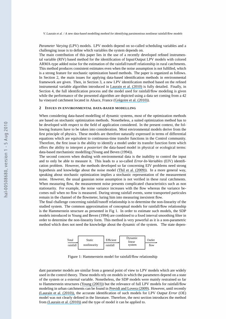
When considering data-based modelling of dynamic systems, most of the optimization methodsare based on stochastic optimization methods. Nonetheless, a suited optimization method has tobe developed with respect to the field of application considered. In the present context, the fol-lowing features have to be taken into consideration. Most environmental models derive from thefirst principle of physics. These models are therefore naturally expressed in terms of differentialequations which are equivalent to continuous-time transfer functions in the Control community.Therefore, the first issue is the ability to identify a model under its transfer function form whichoffers the ability to interpreta posteriori the data-based model in physical or ecological terms:data-based mechanistic modelling (Young and Beven (1994)).The second concern when dealing with environmental data is the inability to control the inputand to only be able to measure it. This leads to a so-calledError-In-Variables (EIV) identifi-cation problem. However, the methods developed so far concerning EIV problems need stronghypothesis and knowledge about the noise model (Thil et al. (2009)). In a more general way,speaking about stochastic optimization implies a stochastic representation of the measurementnoise. However, the usual gaussian noise assumption is not verified in these rural catchments.When measuring flow, the measurement noise presents complicated characteristics such as nonstationarity. For example, the noise variance increases with the flow whereas the variance be-comes null when no flow is measured. During strong rainfall events, some transported particulesremain in the channel of the flowmeter, luring him into measuring inexistent flow.The final challenge concerning rainfall/runoff relationship is to determine the non-linearity of thestudied system. The common approximation of conceptual models for rainfall/flow relationshipis the Hammerstein structure as presented in Fig 1. In order to estimate such models, the SDPmodels introduced in Young and Beven (1994) are combined to afixed interval smoothing filter inorder to determine the non-linearity form. This method is very powerful as it is a non-parametricmethod which does not need the knowledge about the dynamic ofthe system. The state depen-

Total

rainfall

Efficient

rainfall

Outlet

flow

Static

nonlinearity

Dynamiclinearsystem

Figure 1: Hammerstein model for rainfall/flow relationship

dant parameter models are similar from a general point of view to LPV models which are widelyused in the control theory. These models rely on models in which the parameters depend on a stateof the system or a external variable. Nonetheless, the SDP models were mainly restrained so farto Hammerstein structures (Young (2003)) but the relevanceof full LPV models for rainfall/flowmodeling in urban catchments can be found in Previdi and Lovera (2009). However, until recently(Laurain et al. (2010)), the accurate identification of suchmodels for LPVOutput Error (OE)model was not clearly defined in the literature. Therefore, the next section introduces the methodfrom (Laurain et al. (2010)) and the type of model it can be applied to.

hal-0

0508

680,

ver

sion

1 -

5 Au

g 20

10

V. Laurain et al. / A new data-based modelling method for identifying parsimonious nonlinear rainfall/flow models

3 ESTIMATION OF LPV OUTPUT ERROR M ODELS

Would the system be linear, a method dealing robustly with the noise conditions depicted inthe previous section is theSimplified Refined Instrumental Variable(SRIV) method proposed inYoung and Jakeman (1980). Moreover, this method was extended to non-linear models (Laurainet al. (2008)). This section exposes the extension of the SRIV method toLPV-OEmodels: theLPV-SRIV method. In the LPV case, most of the methods developed for Input/output (IO) mod-els based identification are derived under a linear regression form (Wei and Del Re (2006); Giarreet al. (2006); Butcher et al. (2008)). By using the concepts of the Linear Time Invariant(LTI)prediction error framework, recursiveleast squares(LS) andinstrumental variable(IV) methodshave been also introduced (Giarre et al. (2006); Butcher et al. (2008)). A discussion about theperformances and robustness of these algorithms compared to the one introduced in this paper canbe found in Laurain et al. (2010).

3.1 LPV output error models

The considered models in this application are given as:

M

{

A(pk, q−1)χ(tk) = B(pk, q−1)u(tk−d)

y(tk) = χ(tk) + e(tk)(1)

whered is the delay,χ is the noise-free output,u is the input,e is the additive noise with boundedspectral density,y is the noisy output of the system andq is the time-shift operator, i.e.q−iu(tk) =u(tk−i). p are the so-called scheduling variables. For LTI systems, the coefficients ofA andB

are constant in time while they are time-varying depending on p for LPV models.A(pk, q−1) andB(pk, q−1) are polynomials inq−1 of degreena andnb respectively:

A(pk, q−1) = 1 +

na∑

i=1

ai(pk)q−i with ai(pk) = ai,0 +

nα∑

l=1

ai,lfl(pk) i = 1, . . . , na (2)

B(pk, q−1) =

nb∑

j=0

bj(pk)q−i with bj(pk) = bj,0 +

nβ∑

l=1

bj,lgl(pk) j = 0, . . . , nb. (3)

In this parametrization,{fl}nα

l=1 and{gl}nβ

l=1 are functions ofp, with static dependence, allowingthe identifiability of the model (pairwise orthogonal functions for example). It can be noticedthat the knowledge of{ai,l}

na,nα

i=1,l=1 and{bj,l}nb,nβ

j=0,l=0 ensures the knowledge of the full model.Therefore, these model parameters are stacked columnwise in the parameter vectorρ,

ρ =[a1 . . . ana

b0 . . . bnb

]⊤∈ R

nρ , nρ = na(nα + 1) + (nb + 1)(nβ + 1)

ai =[

ai,0 ai,1 . . . ai,nα

]∈ R

nα+1 andbj =[

bj,0 bj,1 . . . bj,nβ

]∈ R

nβ+1.

The model defined by equations (1),(2) and (3) is denoted asLPV-OE.

3.2 Identification problem statement

For models given in (1) and assuming that:• the scheduling variablesp are knowna priori,• the functions{fl}

nα

l=1 and{gl}nβ

l=1 are knowna priori,• the ordersna, nb, nα, nβ andd are knowna priori,

the identification problem can then be stated as follows: given the total rainfall datau and theoutlet flow datay sampled at timestk k = 1..N , estimate the associated parameter vectorρ.

3.3 Reformulation of the model

A way to solve the LPV identification problem is to rewrite thesignal relations of (1) into thefollowing form (Laurain et al. (2010)):

Mρ

χ(tk) +

na∑

i=1

ai,0χ(tk−i)

︸ ︷︷ ︸

F (q−1)χ(tk)

+

na∑

i=1

nα∑

l=1

ai,lfl(pk)χ(tk−i)︸ ︷︷ ︸

χi,l(tk)

=

nb∑

j=0

nβ∑

l=0

bj,lgl(pk)u(tk−d−j︸ ︷︷ ︸

)

uj,l(tk)

y(tk)=χ(tk) + e(tk)

hal-0

0508

680,

ver

sion

1 -

5 Au

g 20

10

V. Laurain et al. / A new data-based modelling method for identifying parsimonious nonlinear rainfall/flow models

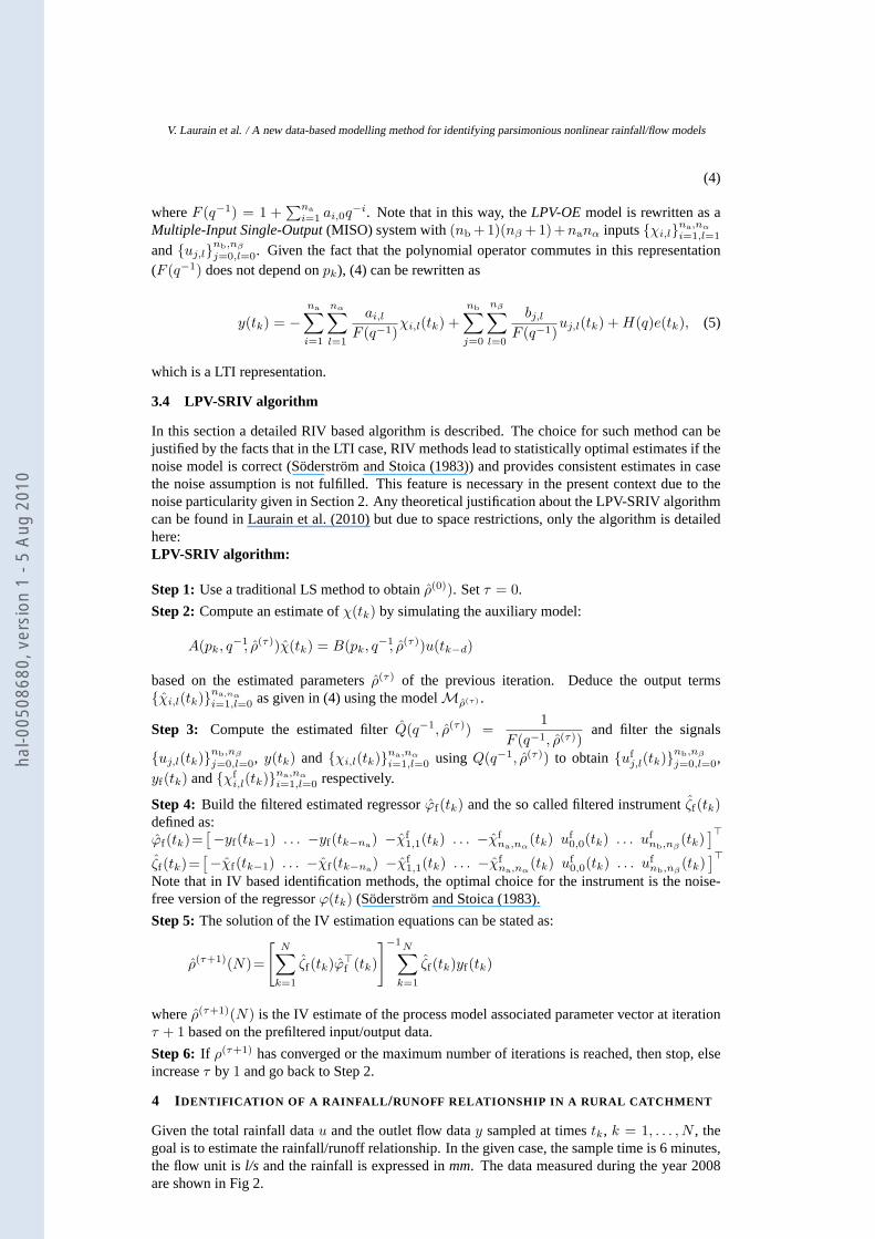
(4)

whereF (q−1) = 1 +∑na

i=1 ai,0q−i. Note that in this way, theLPV-OEmodel is rewritten as a

Multiple-Input Single-Output(MISO) system with(nb +1)(nβ +1)+nanα inputs{χi,l}na,nα

i=1,l=1

and{uj,l}nb,nβ

j=0,l=0. Given the fact that the polynomial operator commutes in this representation(F (q−1) does not depend onpk), (4) can be rewritten as

y(tk) = −

na∑

i=1

nα∑

l=1

ai,l

F (q−1)χi,l(tk) +

nb∑

j=0

nβ∑

l=0

bj,l

F (q−1)uj,l(tk) + H(q)e(tk), (5)

which is a LTI representation.

3.4 LPV-SRIV algorithm

In this section a detailed RIV based algorithm is described.The choice for such method can bejustified by the facts that in the LTI case, RIV methods lead tostatistically optimal estimates if thenoise model is correct (Soderstrom and Stoica (1983)) and provides consistent estimates in casethe noise assumption is not fulfilled. This feature is necessary in the present context due to thenoise particularity given in Section 2. Any theoretical justification about the LPV-SRIV algorithmcan be found in Laurain et al. (2010) but due to space restrictions, only the algorithm is detailedhere:LPV-SRIV algorithm:

Step 1: Use a traditional LS method to obtainρ(0)). Setτ = 0.

Step 2: Compute an estimate ofχ(tk) by simulating the auxiliary model:

A(pk, q−1, ρ(τ))χ(tk) = B(pk, q−1, ρ(τ))u(tk−d)

based on the estimated parametersρ(τ) of the previous iteration. Deduce the output terms{χi,l(tk)}

na,nα

i=1,l=0 as given in (4) using the modelMρ(τ) .

Step 3: Compute the estimated filterQ(q−1, ρ(τ)) =1

F (q−1, ρ(τ))and filter the signals

{uj,l(tk)}nb,nβ

j=0,l=0, y(tk) and {χi,l(tk)}na,nα

i=1,l=0 using Q(q−1, ρ(τ)) to obtain{ufj,l(tk)}

nb,nβ

j=0,l=0,yf(tk) and{χf

i,l(tk)}na,nα

i=1,l=0 respectively.

Step 4: Build the filtered estimated regressorϕf(tk) and the so called filtered instrumentζf(tk)defined as:ϕf(tk)=

[−yf(tk−1) . . . −yf(tk−na

) −χf1,1(tk) . . . −χf

na,nα(tk) uf

0,0(tk) . . . ufnb,nβ

(tk)]⊤

ζf(tk)=[−χf(tk−1) . . . −χf(tk−na

) −χf1,1(tk) . . . −χf

na,nα(tk) uf

0,0(tk) . . . ufnb,nβ

(tk)]⊤

Note that in IV based identification methods, the optimal choice for the instrument is the noise-free version of the regressorϕ(tk) (Soderstrom and Stoica (1983).

Step 5: The solution of the IV estimation equations can be stated as:

ρ(τ+1)(N)=

[N∑

k=1

ζf(tk)ϕ⊤

f (tk)

]−1N∑

k=1

ζf(tk)yf(tk)

whereρ(τ+1)(N) is the IV estimate of the process model associated parametervector at iterationτ + 1 based on the prefiltered input/output data.

Step 6: If ρ(τ+1) has converged or the maximum number of iterations is reached, then stop, elseincreaseτ by 1 and go back to Step 2.

4 IDENTIFICATION OF A RAINFALL /RUNOFF RELATIONSHIP IN A RURAL CATCHMENT

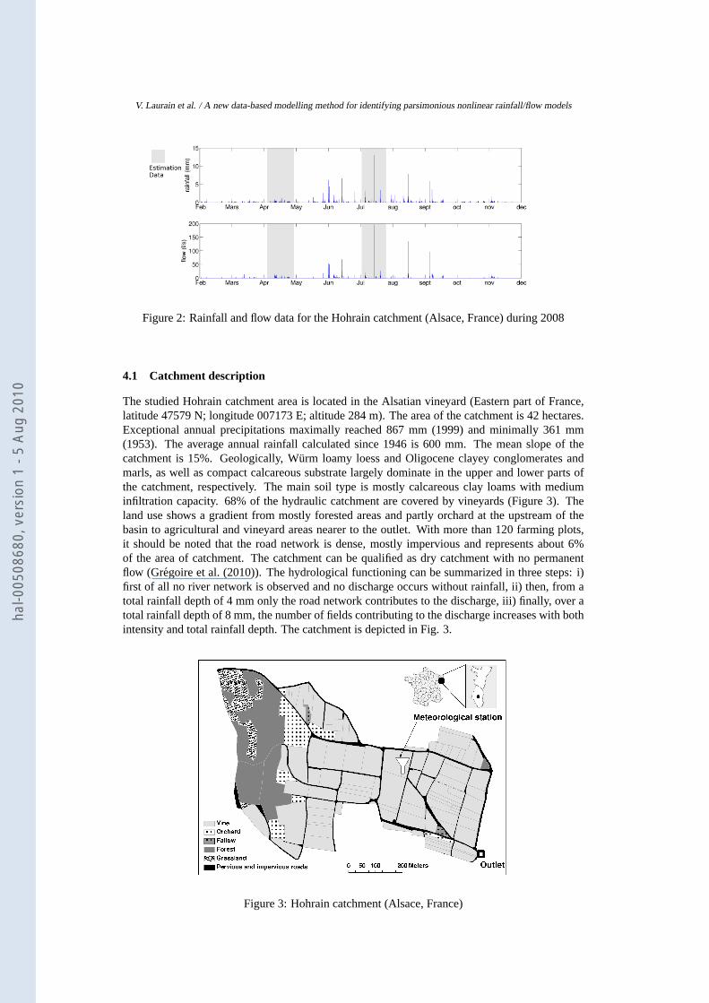
Given the total rainfall datau and the outlet flow datay sampled at timestk, k = 1, . . . , N , thegoal is to estimate the rainfall/runoff relationship. In the given case, the sample time is 6 minutes,the flow unit isl/s and the rainfall is expressed inmm. The data measured during the year 2008are shown in Fig 2.

hal-0

0508

680,

ver

sion

1 -

5 Au

g 20

10

V. Laurain et al. / A new data-based modelling method for identifying parsimonious nonlinear rainfall/flow models

Figure 2: Rainfall and flow data for the Hohrain catchment (Alsace, France) during 2008

4.1 Catchment description

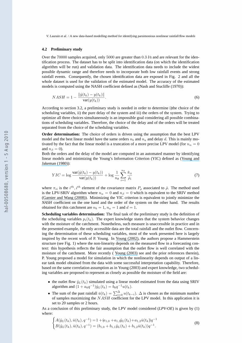
The studied Hohrain catchment area is located in the Alsatian vineyard (Eastern part of France,latitude 47579 N; longitude 007173 E; altitude 284 m). The area of the catchment is 42 hectares.Exceptional annual precipitations maximally reached 867 mm (1999) and minimally 361 mm(1953). The average annual rainfall calculated since 1946 is 600 mm. The mean slope of thecatchment is 15%. Geologically, Wurm loamy loess and Oligocene clayey conglomerates andmarls, as well as compact calcareous substrate largely dominate in the upper and lower parts ofthe catchment, respectively. The main soil type is mostly calcareous clay loams with mediuminfiltration capacity. 68% of the hydraulic catchment are covered by vineyards (Figure 3). Theland use shows a gradient from mostly forested areas and partly orchard at the upstream of thebasin to agricultural and vineyard areas nearer to the outlet. With more than 120 farming plots,it should be noted that the road network is dense, mostly impervious and represents about 6%of the area of catchment. The catchment can be qualified as drycatchment with no permanentflow (Gregoire et al. (2010)). The hydrological functioning can be summarized in three steps: i)first of all no river network is observed and no discharge occurs without rainfall, ii) then, from atotal rainfall depth of 4 mm only the road network contributes to the discharge, iii) finally, over atotal rainfall depth of 8 mm, the number of fields contributing to the discharge increases with bothintensity and total rainfall depth. The catchment is depicted in Fig. 3.

Figure 3: Hohrain catchment (Alsace, France)

hal-0

0508

680,

ver

sion

1 -

5 Au

g 20

10

V. Laurain et al. / A new data-based modelling method for identifying parsimonious nonlinear rainfall/flow models

4.2 Preliminary study

Over the70000 samples acquired, only5000 are greater than0.3 l/s and are relevant for the iden-tification process. The dataset has to be split into identification data (on which the identificationalgorithm will be run) and validation data. The identification data needs to include the widestpossible dynamic range and therefore needs to incorporate both low rainfall events and strongrainfall events. Consequently, the chosen identification data are exposed in Fig. 2 and all thewhole dataset is used for the validation of the estimated model. The accuracy of the estimatedmodels is computed using the NASH coefficient defined as (Nashand Stucliffe (1970)):

NASH = 1 −‖y(tk) − y(tk)‖

var(y(tk)). (6)

According to section 3.2, a preliminary study is needed in order to determine i)the choice of thescheduling variables, ii) the pure delay of the system and iii) the orders of the system. Trying tooptimize all three choices simultaneously is an impossiblegoal considering all possible combina-tions of scheduling variables. Therefore, the choice of thedelay and of the orders will be treatedseparated from the choice of the scheduling variables.

Order determination: The choice of orders is driven using the assumption that the best LPVmodel and the best linear model have the same ordersnb andna and delayd. This is mainly mo-tivated by the fact that the linear model is a truncation of a more precise LPV model (fornα = 0andnβ = 0).Both the orders and the delay of the model are computed in an automated manner by identifyinglinear models and minimizing the Young’s Information Criterion (YIC) defined as (Young andJakeman (1980)):

Y IC = logvar(y(tk) − y(tk))

var(y(tk))+ log

1

nθ

nθ∑

i=1

πii

ρi

(7)

whereπii is theith, ith element of the covariance matrixPρ associated toρ. The method usedis the LPV-SRIV algorithm wherenα = 0 andnβ = 0 which is equivalent to the SRIV method(Garnier and Wang (2008)). Minimizing the YIC criterion is equivalent to jointly minimize theNASHcoefficient on the one hand and the order of the system on the other hand. The resultsobtained for this catchment arenb = 1, na = 1 andd = 1.

Scheduling variables determination:The final task of the preliminary study is the definition ofthe scheduling variablespi(tk). The expert knowledge states that the system behavior changeswith the moisture of the catchment. Nonetheless, such measure is unaccessible in practice and inthe presented example, the only accessible data are the total rainfall and the outlet flow. Concern-ing the determination of these scheduling variables, most of the work presented here is largelyinspired by the recent work of P. Young. In Young (2002), the authors propose a Hammersteinstructure (see Fig. 1) where the non-linearity depends on the measured flow in a forecasting con-text: this hypothesis reflects the fair assumption that the outlet flow is well correlated with themoisture of the catchment. More recently ( Young (2003) see and the prior references therein),P. Young proposed a model for simulation in which the nonlinearity depends on output of a lin-ear tank model obtained from the data with some successful interpretation capability. Therefore,based on the same correlation assumption as in Young (2003) and expert knowledge, two schedul-ing variables are proposed to represent as closely as possible the moisture of the field are:

• the outlet flowyL(tk) simulated using a linear model estimated from the data usingSRIValgorithm and(1 + a0q

−1)yL(tk) = b0q−1u(tk).

• The sum of the past rainfallu(tk) =∑∆

i=0 u(tk−i). ∆ is chosen as the minimum numberof samples maximizing theNASH coefficient for the LPV model. In this application it isset to 20 samples or 2 hours.

As a conclusion of this preliminary study, the LPV model considered (LPV-OE) is given by (1)where:

{

A(yL(tk), u(tk), q−1) =1 +(a1,0 +a1,1yL(tk)+a1,2u(tk))q−1

B(yL(tk), u(tk), q−1) = (b1,0 + b1,1yL(tk) + b1,2u(tk))q−1.(8)

hal-0

0508

680,

ver

sion

1 -

5 Au

g 20

10

V. Laurain et al. / A new data-based modelling method for identifying parsimonious nonlinear rainfall/flow models

4.3 Results

In this section, the results exposed will focus in showing i)the relevance of the LPV model and ii)the relevance of using a consistent method for unknown noisestructure. Therefore, the presentedalgorithm will be compared to LS based methods which assumeAuto Regressive models witheXogenous inputs(ARX) where the noise has the same dynamic as the system, whether it is alinear model (ARX),

(1 + a0q−1)y(tk) = b0q

−1u(tk) + e(tk), (9)

or a LPV model (LPV-ARX)

A(yL(tk), u(tk), q−1)y(tk) = B(yL(tk), u(tk), q−1)u(tk) + e(tk). (10)

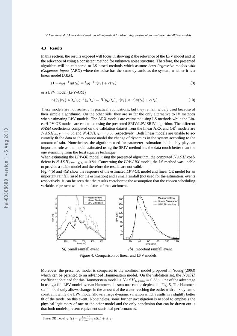
These models are not realistic in practical applications, but they remain widely used because oftheir simple algorithmic. On the other side, they are so far the only alternative to IV methodswhen estimating LPV models. The ARX models are estimated using LS methods while the Lin-ear/LPV OE models are estimated using the presented SRIV/LPV-SRIV algorithm. The differentNASHcoefficients computed on the validation dataset from the linear ARX and OE1 models areNASHARX = 0.54 andNASHOE = 0.63 respectively. Both linear models are unable to ac-curately fit the data as they cannot model the change of dynamics in the system according to theamount of rain. Nonetheless, the algorithm used for parameter estimation indubitably plays animportant role as the model estimated using the SRIV method fits the data much better than theone stemming from the least squares technique.When estimating theLPV-OEmodel, using the presented algorithm, the computedNASH coef-ficient isNASHLPV −OE = 0.84. Concerning theLPV-ARXmodel, the LS method was unableto provide a stable model and therefore the results are not valid.Fig. 4(b) and 4(a) show the response of the estimatedLPV-OEmodel and linear OE model for animportant rainfall (used for the estimation) and a small rainfall (not used for the estimation) eventsrespectively. It can be seen that the results corroborate the assumption that the chosen schedulingvariables represent well the moisture of the catchment.

100 200 300 400 5000

2

4

6

8

10

12

14

16

18

time (min)

flow

(l/s

)

Measured flowLinear SimulationLPV Simulation

(a) Small rainfall event

20 40 60 80 100 120

20

40

60

80

100

120

140

160

180

time (min)

flow

(l/s

)

Measured flowLinear SimulationLPV Simulation

(b) Important rainfall event

Figure 4: Comparison of linear and LPV models

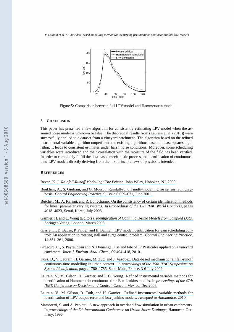
Moreover, the presented model is compared to the nonlinear model proposed in Young (2003)which can be parented to an advanced Hammerstein model. On the validation set, theNASH

coefficient obtained for this Hammerstein model isNASHHamm = 0.835. One of the advantagein using a full LPV model over an Hammerstein structure can bedepicted in Fig. 5. The Hammer-stein model only allows changes in the amount of the water reaching the outlet with a fix dynamicconstraint while the LPV model allows a large dynamic variation which results in a slightly betterfit of the model on this event. Nonetheless, some further investigation is needed to emphasis thephysical legitimacy of one or the other model and the only conclusion that can be drawn out isthat both models present equivalent statistical performances.

1Linear OE model:y(tk) = b0q−1

(1+a0q−1)u(tk) + e(tk)

hal-0

0508

680,

ver

sion

1 -

5 Au

g 20

10

V. Laurain et al. / A new data-based modelling method for identifying parsimonious nonlinear rainfall/flow models

20 40 60 80 100 120

50

100

150

200

time (min)

flow

(l/s

)

Measured flowHammerstein SimulationLPV Simulation

Figure 5: Comparison between full LPV model and Hammersteinmodel

5 CONCLUSION

This paper has presented a new algorithm for consistently estimating LPV model when the as-sumed noise model is unknown or false. The theoretical results from (Laurain et al. (2010)) weresuccessfully applied to a dataset from a vineyard catchment. The algorithm based on the refinedinstrumental variable algorithm outperforms the existingalgorithms based on least squares algo-rithm: it leads to consistent estimates under harsh noise conditions. Moreover, some schedulingvariables were introduced and their correlation with the moisture of the field has been verified.In order to completely fulfill the data-based mechanistic process, the identification of continuous-time LPV models directly deriving from the first principle laws of physics is intended.

REFERENCES

Beven, K. J.Rainfall-Runoff Modelling: The Primer. John Wiley, Hoboken, NJ, 2000.

Boukhris, A., S. Giuliani, and G. Mourot. Rainfall-runoff multi-modelling for sensor fault diag-nosis.Control Engineering Practice, 9, Issue 6:659–671, June 2001.

Butcher, M., A. Karimi, and R. Longchamp. On the consistencyof certain identification methodsfor linear parameter varying systems. InProceedings of the 17th IFAC World Congress, pages4018–4023, Seoul, Korea, July 2008.

Garnier, H. and L. Wang (Editors).Identification of Continuous-time Models from Sampled Data.Springer-Verlag, London, March 2008.

Giarre, L., D. Bauso, P. Falugi, and B. Bamieh. LPV model identification for gain scheduling con-trol: An application to rotating stall and surge control problem. Control Engineering Practice,14:351–361, 2006.

Gregoire, C., S. Payraudeau and N. Domange. Use and fate of 17 Pesticides applied on a vineyardcatchment.Inter. J. Environ. Anal. Chem., 09:404–418, 2010.

Kuss, D., V. Laurain, H. Garnier, M. Zug, and J. Vazquez. Data-based mechanistic rainfall-runoffcontinuous-time modelling in urban context. Inproceedings of the 15th IFAC Symposium onSystem Identification, pages 1780–1785, Saint-Malo, France, 3-6 July 2009.

Laurain, V., M. Gilson, H. Garnier, and P. C. Young. Refined instrumental variable methods foridentification of Hammerstein continuous time Box-Jenkinsmodels. Inproceedings of the 47thIEEE Conference on Decision and Control, Cancun, Mexico, Dec 2008.

Laurain, V., M. Gilson, R. Toth, and H. Garnier. Refined instrumental variable methods foridentification of LPV output-error and box-jenkins models.Accepted to Automatica, 2010.

Mambretti, S. and A. Paoletti. A new approach in overland flowsimulation in urban catchments.In proceedings of the 7th International Conference on Urban Storm Drainage, Hannover, Ger-many, 1996.

hal-0

0508

680,

ver

sion

1 -

5 Au

g 20

10

V. Laurain et al. / A new data-based modelling method for identifying parsimonious nonlinear rainfall/flow models

Nash, J. and J. Stucliffe. River flow forecasting through conceptuel models. part 1-a discussion ofprinciples.Journal of Hydrology, 10, Issue 3:282–290, 1970.

Previdi, F. and M. Lovera. Identification of parametrically- varying models for the rainfall-runoffrelationship in urban drainage networks. Inproceedings of the 15th IFAC Symposium on SystemIdentification, pages 1768–1773, Saint-Malo, France, 3-6 July 2009.

Previdi, F., M. Lovera, and S. Mambretti. Identification of the rainfall-runoff relationship in urbandrainage networks.Control Engineering Practice, 7, Issue 12:1489–1504, 1999.

Soderstrom, T. and P. Stoica.Instrumental Variable Methods for System Identification. Springer-Verlag, New York, 1983.

Thil, S., W. Zheng, M. Gilson, and H. Garnier. Unifying some higher-order statistic-based meth-ods for errors-in-variables model identification.Automatica, 45, Issue 8:1937–1942, August2009.

Wei, X. and L. Del Re. On persistent excitation for parameterestimation of quasi-LPV systemsand its application in modeling of diesel engine torque. InProceedings of the 14th IFAC Sym-posium on System Identification, pages 517–522, Newcastle, Australia, March 2006.

Young, P. C. and A. Jakeman. Refined instrumental variable methods of recursive time-seriesanalysis - part III. extensions.International Journal of Control, 31, Issue 4:741–764, 1980.

Young, P. and K. Beven. Data-based mechanistic modelling and the rainfall-flow non-linearity.Environmetrics, 5:335–363, 1994.

Young, P. C. Advances on real-time flood forecastingPhil. Trans. of the Royal Society, 360, no.1796:1433–1450, 2002.

Young, P. C. Top-down ad data-based mechanistic modelling of rainfall-flow dynamics at thecatchment scale.Hydrological processes, 17:2195–2217, 2003.

Young, P. C. and H. Garnier. Identification and estimation ofcontinuous-time, data-based mech-anistic (DBM) models for environmental systems.Environmental Modelling & Software, 21,Issue 8:1055–1072, August 2006.

hal-0

0508

680,

ver

sion

1 -

5 Au

g 20

10