Jawaharlal Nehru Technological University Hyderabad Master Thesis A New Approach to Design and Implement FFT / IFFT Processor Based on Radix-4 2 Algorithm Author: Parunandula Shravankumar Supervisor: Mr. Srujan Gaddam A thesis submitted in fulfilment of the requirements for the degree of Master of Technology in the Department of Electronics and Communication Engineering Aurora’s Scientific, Technological & Research Academy December 2014

Welcome message from author
This document is posted to help you gain knowledge. Please leave a comment to let me know what you think about it! Share it to your friends and learn new things together.
Transcript
Jawaharlal Nehru TechnologicalUniversity Hyderabad
Master Thesis
A New Approach to Design andImplement FFT / IFFT Processor
Based on Radix-42 Algorithm
Author:
Parunandula
Shravankumar
Supervisor:
Mr. Srujan Gaddam
A thesis submitted in fulfilment of the requirements
for the degree of Master of Technology
in the
Department of Electronics and Communication
Engineering
Aurora’s Scientific, Technological & Research Academy
December 2014

Declaration of Authorship
I, Parunandula Shravankumar, declare that this thesis titled, ’A New Approach
to Design and Implement FFT / IFFT Processor Based on Radix-42 Algorithm’
and the work presented in it are my own. I confirm that:
This work was done wholly or mainly while in candidature for a research
degree at this University.
Where any part of this thesis has previously been submitted for a degree or
any other qualification at this University or any other institution, this has
been clearly stated.
Where I have consulted the published work of others, this is always clearly
attributed.
Where I have quoted from the work of others, the source is always given.
With the exception of such quotations, this thesis is entirely my own work.
I have acknowledged all main sources of help.
Where the thesis is based on work done by myself jointly with others, I have
made clear exactly what was done by others and what I have contributed
myself.
Signed:
Date:
i

Abstract
Fast Fourier Transform (FFT) processing is an important component of many
Digital Signal Processing (DSP) applications and communication systems. This
thesis focused on Algorithm development, mathematical analysis, High Level Syn-
thesis, and C/C++ prototyping. A new approach to design and implement Fast
Fourier Transform(FFT) using Radix-42 algorithm ,and how the multidimensional
index mapping reduces the complexity of FFT computation are Proposed and Dis-
cussed in an easy understanding manner. Using mathematical analysis on radix-4
DFT(Discrete Fourier Transform) kernel, the formal radix-4 butterfly structure is
remodeled.
This makes the design perspective so simple to implement the mathematical algo-
rithm into hardware realization model. The cost of the processor is proportional to
the cost of the constant multipliers. So, to reduce the cost of constant multipliers,
we reduced the phase factor storage for the entire range of N-point sequence to
increase the FFT Computation efficiency.
A clear and straight analysis has done and described, two approaches are given
to implement the FFT algorithm, One is hardware generation using MATLAB-
Simulink and the other is C / C++ prototype. Also compared the speeds of MEX
(Matlab Executable) C code vs. MATLAB .m function.High level synthesis has
done using Simulink and shown the reduced number of computation in terms of
Multipliers and Add / Sub tractors.

Contents
Declaration of Authorship i
Abstract ii
Contents iii
List of Figures vi
List of Tables viii
Abbreviations ix
Symbols x
1 Introduction 1
1.1 Aim of the Project . . . . . . . . . . . . . . . . . . . . . . . . . . . 2
1.2 Problem Definition . . . . . . . . . . . . . . . . . . . . . . . . . . . 4
1.3 Motivation . . . . . . . . . . . . . . . . . . . . . . . . . . . . . . . . 4
1.4 Organization of Thesis . . . . . . . . . . . . . . . . . . . . . . . . . 10
2 Literature survey 11
3 Theoretical Analysis 14
3.1 Efficient Computation of the DFT : FFT Algorithms . . . . . . . . 14
3.1.1 Defination of DFT . . . . . . . . . . . . . . . . . . . . . . . 15
3.1.2 Inverse DFT . . . . . . . . . . . . . . . . . . . . . . . . . . . 16
3.2 Mathematics of DFT . . . . . . . . . . . . . . . . . . . . . . . . . . 16
3.2.1 Orthogonality of Sinusoids . . . . . . . . . . . . . . . . . . . 18
3.2.2 Nth Roots of Unity . . . . . . . . . . . . . . . . . . . . . . . 19
3.2.3 DFT Sinusoids . . . . . . . . . . . . . . . . . . . . . . . . . 19
3.3 Mixed-Radix Cooley-Tukey FFT . . . . . . . . . . . . . . . . . . . 20
3.3.1 Divide-and-Conquer Approach to Computation of the DFT . 22
iii
Contents iv
3.3.2 Decimation in Time FFT Algorithms . . . . . . . . . . . . . 25
3.3.3 Radix 2 FFT Algorithm . . . . . . . . . . . . . . . . . . . . 26
3.3.4 Computational cost of radix-2 DIT FFT . . . . . . . . . . . 28
3.4 Prime Factor Algorithm (PFA) . . . . . . . . . . . . . . . . . . . . 28
3.5 Radix-4 FFT Algorithms . . . . . . . . . . . . . . . . . . . . . . . . 29
3.5.1 Radix-4 FFT Operation Counts . . . . . . . . . . . . . . . . 35
4 Experimental Investigations 36
4.1 Understanding the FFT . . . . . . . . . . . . . . . . . . . . . . . . 36
4.1.1 Phase factors / Twiddle factors . . . . . . . . . . . . . . . . 36
4.1.2 Multi-Dimensional Index Mapping . . . . . . . . . . . . . . 38
4.1.3 Index Mapping . . . . . . . . . . . . . . . . . . . . . . . . . 38
4.2 Radix-42 FFT/IFFT Algorithm . . . . . . . . . . . . . . . . . . . . 39
4.3 Implementation of the Processing Element . . . . . . . . . . . . . . 41
4.4 FFT Design Using Simulink . . . . . . . . . . . . . . . . . . . . . . 45
4.4.1 Simulink . . . . . . . . . . . . . . . . . . . . . . . . . . . . . 45
4.4.2 Generating HDL Code . . . . . . . . . . . . . . . . . . . . . 46
4.4.3 HDL Code Generation from MATLAB . . . . . . . . . . . . 46
4.4.4 HDL Code Generation from Simulink . . . . . . . . . . . . . 47
4.4.5 Model Designing . . . . . . . . . . . . . . . . . . . . . . . . 47
5 Experimental Results 54
5.1 Prototyping as C/C++ Code . . . . . . . . . . . . . . . . . . . . . 54
5.1.1 Use Cases . . . . . . . . . . . . . . . . . . . . . . . . . . . . 55
5.1.2 Motivations . . . . . . . . . . . . . . . . . . . . . . . . . . . 56
5.1.3 Requirements . . . . . . . . . . . . . . . . . . . . . . . . . . 56
5.2 C Code Generation using MATLAB Coder . . . . . . . . . . . . . . 57
5.2.1 Main function . . . . . . . . . . . . . . . . . . . . . . . . . . 57
5.2.2 Testbench . . . . . . . . . . . . . . . . . . . . . . . . . . . . 60
5.2.3 Running MEX and Code Generation . . . . . . . . . . . . . 62
6 Discussion of Results 68
6.1 Profiling . . . . . . . . . . . . . . . . . . . . . . . . . . . . . . . . . 68
6.2 Profile Summary . . . . . . . . . . . . . . . . . . . . . . . . . . . . 69
6.2.1 MEX vs. .m function . . . . . . . . . . . . . . . . . . . . . . 72
7 Summery,Conclusion and Reccomendations 75
7.1 summary . . . . . . . . . . . . . . . . . . . . . . . . . . . . . . . . . 75
7.2 Conclusion . . . . . . . . . . . . . . . . . . . . . . . . . . . . . . . . 76
7.3 Future Work . . . . . . . . . . . . . . . . . . . . . . . . . . . . . . . 76
Contents v
A MATLAB Functions, Codes and Test-benches 77
A.1 MATLAB function of fftx N . . . . . . . . . . . . . . . . . . . . . . 77
A.2 Code generation for function ’fftx N’ . . . . . . . . . . . . . . . . . 82
A.3 Processing Element.vhd . . . . . . . . . . . . . . . . . . . . . . . . 91
A.4 Processing Element tb.vhd . . . . . . . . . . . . . . . . . . . . . . . 96
Bibliography 117

List of Figures
3.1 N throots of Unity . . . . . . . . . . . . . . . . . . . . . . . . . . . . 20
3.2 Sinusoids . . . . . . . . . . . . . . . . . . . . . . . . . . . . . . . . . 21
3.3 Decimation-in-Time . . . . . . . . . . . . . . . . . . . . . . . . . . . 27
3.4 Radix-4 FFT Butterfly Structure:Basic butterfly computation in aradix-4 FFT algorithm . . . . . . . . . . . . . . . . . . . . . . . . . 31
3.5 Radix-4 FFT Butterfly Structure:16-point radix-4 decimation-in-time algorithm . . . . . . . . . . . . . . . . . . . . . . . . . . . . . 32
3.6 Radix-4 FFT Butterfly Structure:16-point radix-4 decimation-in-frequency algorithm . . . . . . . . . . . . . . . . . . . . . . . . . . . 34
4.1 Multi-Dimensional array structure . . . . . . . . . . . . . . . . . . . 38
4.2 Proposed Butterfly Structure . . . . . . . . . . . . . . . . . . . . . 43
4.3 Simulink Model of Proposed Butterfly structure . . . . . . . . . . . 43
4.4 Radix-4 FFT Simulink Model . . . . . . . . . . . . . . . . . . . . . 48
4.5 Radix-4 FFT Simulink Model Processing Element : First Stage . . 48
4.6 List variables in workspace, with sizes and types . . . . . . . . . . . 49
4.7 Radix-4 FFT Simulink Model : Second Stage . . . . . . . . . . . . . 50
4.8 Radix-4 FFT Simulink Model : Third Stage . . . . . . . . . . . . . 51
4.9 HDL Coder Workflow Advisor for Simulink. . . . . . . . . . . . . . 52
4.10 Resource Utilization report . . . . . . . . . . . . . . . . . . . . . . . 52
4.11 HDL Code Generation Summary . . . . . . . . . . . . . . . . . . . 53
5.1 MATLAB Coder Project:Checking Code Generation Readiness . . . 59
5.2 MATLAB Coder Project:Starting a new Project . . . . . . . . . . . 59
5.3 MATLAB Coder Project:Overview . . . . . . . . . . . . . . . . . . 60
5.4 MATLAB Coder Project:Adding Files to MATLAB Coder . . . . . 60
5.5 MATLAB Coder Project:Defining the Variables . . . . . . . . . . . 61
5.6 MATLAB Coder Project:Running for MEX . . . . . . . . . . . . . 61
5.7 MATLAB Coder Project:Static Library . . . . . . . . . . . . . . . 63
5.8 FFTx N: Output of MEX 256-point . . . . . . . . . . . . . . . . . . 64
5.9 MATLAB Coder Project:Building the Code for Project . . . . . . . 65
5.10 MATLAB Coder Project:Some lines of the Generated C Code . . . 66
5.11 MATLAB Coder Project:Static Code Metrics Report . . . . . . . . 66
vi
List of Figures vii
5.12 MATLAB Code Project:C files Generated . . . . . . . . . . . . . . 67
6.1 Profile Summary : Profile Summary unoptimized . . . . . . . . . . 70
6.2 Profile Summary: Function Listing unoptimized . . . . . . . . . . . 71
6.3 Profile Summary . . . . . . . . . . . . . . . . . . . . . . . . . . . . 72
6.4 Profile Summary: Function Listing . . . . . . . . . . . . . . . . . . 72
6.5 Lines where the most time was spent . . . . . . . . . . . . . . . . . 73
6.6 Spectrum: FFT . . . . . . . . . . . . . . . . . . . . . . . . . . . . 74
6.7 MEX:Lines where the most time was spent . . . . . . . . . . . . . . 74
6.8 Lines where the most time was spent MEX vs. Function . . . . . . 74
List of Tables
4.1 Twiddle Factors : W16 . . . . . . . . . . . . . . . . . . . . . . . . . 50
viii
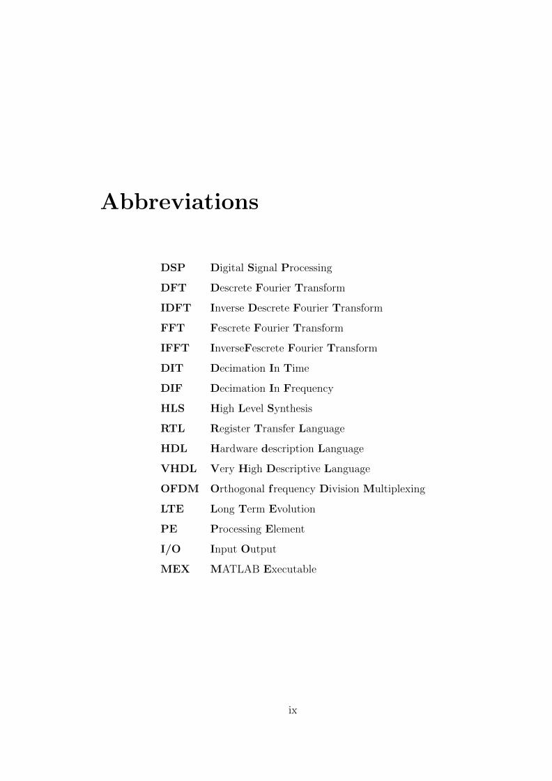
Abbreviations
DSP Digital Signal Processing
DFT Descrete Fourier Transform
IDFT Inverse Descrete Fourier Transform
FFT Fescrete Fourier Transform
IFFT InverseFescrete Fourier Transform
DIT Decimation In Time
DIF Decimation In Frequency
HLS High Level Synthesis
RTL Register Transfer Language
HDL Hardware description Language
VHDL Very High Descriptive Language
OFDM Orthogonal frequency Division Multiplexing
LTE Long Term Evolution
PE Processing Element
I/O Input Output
MEX MATLAB Executable
ix

Symbols
i or j Imaginry Unit
W or ω Twiddle Factor
x

Chapter 1
Introduction
The fast Fourier transform (FFT) has become well known as a very efficient al-
gorithm for calculating the discrete Fourier transform (DFT) of the sequence of
N numbers. The DFT plays an important role in the analysis, design, and imple-
mentation of discrete-time signal-processing algorithms and systems. The DFT is
used in many disciplines to obtain the spectrum or frequency content of a Signal,
and to facilitate the computation of discrete convolution and correlation. The fast
Fourier transform (FFT) is a fundamental problem-solving tool in the educational,
industrial, and military sectors. Since 1965,FFT usage has rapidly expanded and
personal computers fuel an explosion of additional FFT applications. The FFT
is certainly ubiquitous because of the great variety of apparent unrelated fields of
applications, However, we know that the proliferation of applications across broad
and diverse areas is because they are united by a common entity, the Fourier Trans-
form. For years only the elitist theoretical mathematician was capable of staying
abreast of such a broad spectrum of technologies. However, with the FFT, Fourier
analysis has been reduced to readily available and practical procedure that can be
applied effectively without sophisticated training or years of experience. The FFT
has become a standard analysis module because of its usefulness and availability.
1
Chapter 1. Introduction 2
The Next portable devices such as smart phone, tablet, personal digital assistant
demand high transmission bandwidth and high communication quality[1].FFT
processors have been extensively used in various applications such as communi-
cations, image, and bio-medical signal processing.For example, high performance
and low power FFT processing are imperative in Orthogonal Frequency Division
Multiplexing (OFDM) based Communication systems, as a programmable base
band processor for multiple radio standards, including the wireless LAN stan-
dards 802.11a and 802.11b. 802.11a is based on OFDM and uses a 64-point FFT.
The WiMAX also base band is constructed around OFDM technology requiring
high processing throughput. The fixed, IEEE 802.16e version of WiMAX also
needs a 256-point FFT computation.[2]
1.1 Aim of the Project
An increasing number of ASIC designs are based on highly mathematical algo-
rithms. Why?
Media-processing systems, which contain wireless communications, imaging or au-
dio processing, are all based on mathematical algorithms. These systems require a
unique design process that start with the initial description of the algorithm and
continuing to the final implementation.
Getting the algorithm right and implementing it on the right mix of hardware and
software is the key to a successful system. The implementation decisions start at
the architectural level. To ensure design success, however, the high-level model
must be tightly coupled to the implementation design flow. More implementation
detail needs to be brought into the algorithmic design. Trade-offs can then be
made at a higher level. In addition, more implementation detail needs to be
passed to the register-transfer-level (RTL), verification, and software engineers.
They’ll start from a firmer footing as they begin to create the realizable description
Chapter 1. Introduction 3
of the system. Media-processing systems are signal-processing-centric. Consider
Ultra Wideband (UWB), 802.11n, or H.264. The signal-processing algorithm is
the intellectual core of the design. The complex mathematical algorithm must be
described at a high level so that it can be thoroughly characterized and optimized
for mathematical accuracy. The algorithm design language of choice is MATLAB
from The Mathworks.
Initially, there isn’t a distinction between the hardware and software portions of
the algorithm. It’s possible that the entire algorithm will be implemented as an
application-specific integrated circuit (ASIC). It also is possible that the algorithm
will be implemented as software executing on a standard digital signal processor
(DSP). For our discussion, let’s consider a common case for sophisticated signal-
processing systems: Part of the algorithm becomes custom RTL while another
part executes on an embedded core.
For mathematical accuracy, holistic design is important. The whole algorithm
must be completely characterized before it can be divided. Usually, a small group
of system architects starts by creating a MATLAB model of the algorithm. The
initial algorithm that’s described is an idealized floating-point model. Extensive
simulations are executed to characterize the mathematical behavior.
To become an end product, this algorithm will have to go through multiple tran-
sitions. Being able to reproducibly go from the high-level description of the ideal
behavior to implementable RTL or deployable C is fundamentally important to the
design process. To make accurate tradeoffs at the implementation level, system ar-
chitects need a reliable way to go from MATLAB to either RTL or C. In addition,
implementation engineers need accurate guidance on the algorithm’s technology
requirements.
We have many Algorithms and Architectures to compute FFT. In this project we
have mainly concentrated on Radix-42 FFT algorithm and it’s implementation.We
Chapter 1. Introduction 4
used Matlabr and Simulinkr to develop the model and algorithm also used for
testing.
1.2 Problem Definition
The direct DFT calculation is computationally quite “ expensive ” — meaning
that the time taken to compute the result is signifi cant when compared with the
sample period. Not only is a faster method desirable, in real - time applications,
it is essential. This section describes the so - called FFT, which substantially
reduces the computation required to produce exactly the same result as the DFT.
The FFT is a key algorithm in many signal processing areas today. This is because
its use extends far beyond simple frequency analysis — it may be used in a number
of “ fast ” algorithms for fi ltering and other transformations. As such, a solid
understanding of the FFT is well worth the intellectual effort.
1.3 Motivation
Why is the Fourier transform so important?
It indeed is quite hard to pinpoint why exactly Fourier transforms are important
in signal processing. The simplest, hand waving answer one can provide is that it
is an extremely powerful mathematical tool that allows you to view your signals
in a different domain, inside which several difficult problems become very simple
to analyze.
Its ubiquity in nearly every field of engineering and physical sciences, all for dif-
ferent reasons, makes it all the more harder to narrow down a reason. I hope that
looking at some of its properties which led to its widespread adoption along with
Chapter 1. Introduction 5
some practical examples and a dash of history might help one to understand its
importance.
History:
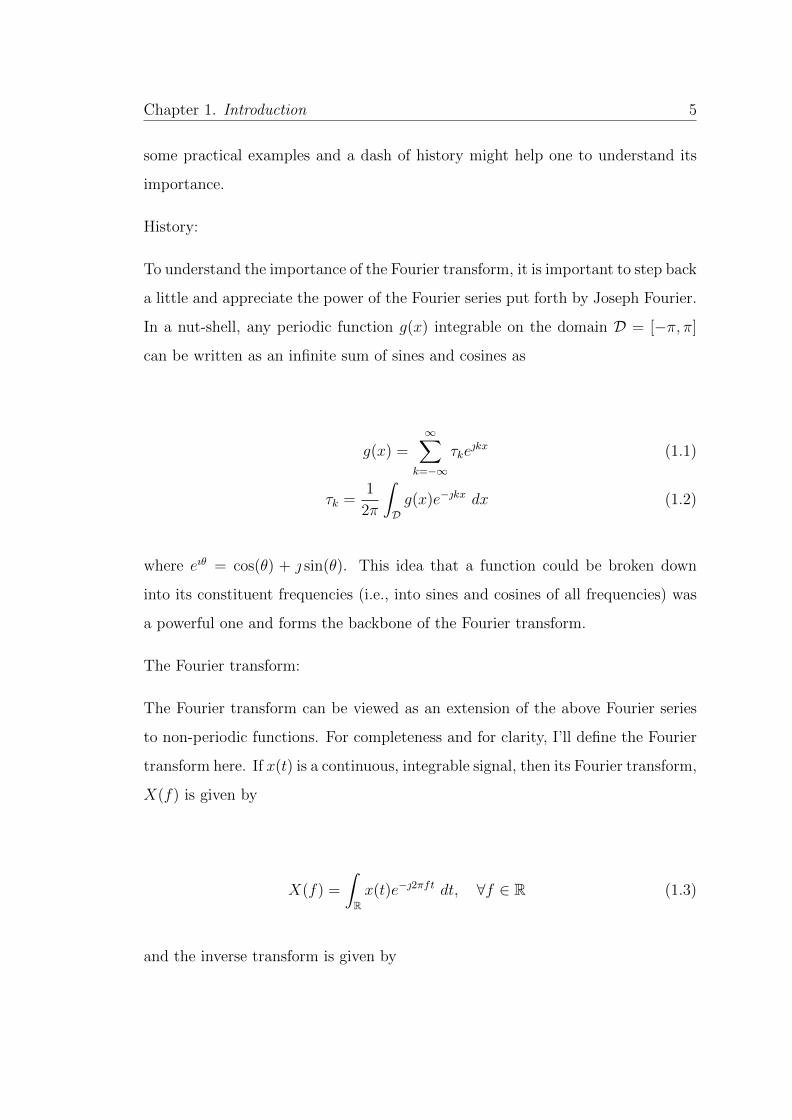
To understand the importance of the Fourier transform, it is important to step back
a little and appreciate the power of the Fourier series put forth by Joseph Fourier.
In a nut-shell, any periodic function g(x) integrable on the domain D = [−π, π]
can be written as an infinite sum of sines and cosines as
g(x) =∞∑
k=−∞
τkekx (1.1)
τk =1
2π
∫Dg(x)e−kx dx (1.2)
where eıθ = cos(θ) + sin(θ). This idea that a function could be broken down
into its constituent frequencies (i.e., into sines and cosines of all frequencies) was
a powerful one and forms the backbone of the Fourier transform.
The Fourier transform:
The Fourier transform can be viewed as an extension of the above Fourier series
to non-periodic functions. For completeness and for clarity, I’ll define the Fourier
transform here. If x(t) is a continuous, integrable signal, then its Fourier transform,
X(f) is given by
X(f) =
∫Rx(t)e−2πft dt, ∀f ∈ R (1.3)
and the inverse transform is given by
Chapter 1. Introduction 6
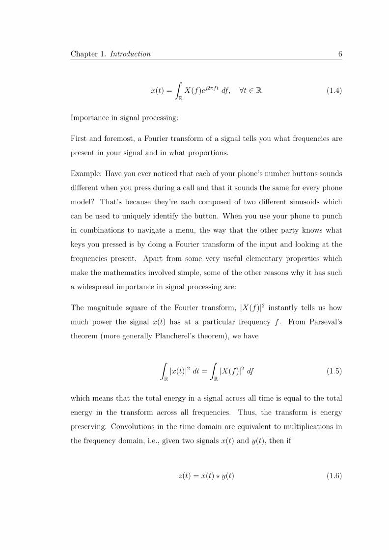
x(t) =
∫RX(f)e2πft df, ∀t ∈ R (1.4)
Importance in signal processing:
First and foremost, a Fourier transform of a signal tells you what frequencies are
present in your signal and in what proportions.
Example: Have you ever noticed that each of your phone’s number buttons sounds
different when you press during a call and that it sounds the same for every phone
model? That’s because they’re each composed of two different sinusoids which
can be used to uniquely identify the button. When you use your phone to punch
in combinations to navigate a menu, the way that the other party knows what
keys you pressed is by doing a Fourier transform of the input and looking at the
frequencies present. Apart from some very useful elementary properties which
make the mathematics involved simple, some of the other reasons why it has such
a widespread importance in signal processing are:
The magnitude square of the Fourier transform, |X(f)|2 instantly tells us how
much power the signal x(t) has at a particular frequency f . From Parseval’s
theorem (more generally Plancherel’s theorem), we have
∫R|x(t)|2 dt =
∫R|X(f)|2 df (1.5)
which means that the total energy in a signal across all time is equal to the total
energy in the transform across all frequencies. Thus, the transform is energy
preserving. Convolutions in the time domain are equivalent to multiplications in
the frequency domain, i.e., given two signals x(t) and y(t), then if
z(t) = x(t) ? y(t) (1.6)

Chapter 1. Introduction 7
where ? denotes convolution, then the Fourier transform of z(t) is merely
Z(f) = X(f) · Y (f) (1.7)
For discrete signals, with the development of efficient FFT algorithms, almost
always, it is faster to implement a convolution operation in the frequency domain
than in the time domain.
Similar to the convolution operation, cross-correlations are also easily implemented
in the frequency domain as Z(f) = X(f)∗Y (f), where ∗ denotes complex conju-
gate. By being able to split signals into their constituent frequencies, one can
easily block out certain frequencies selectively by nullifying their contributions.
Example: When a wave travels through a heterogenous medium, it slows down and
speeds up according to changes in the speed of wave propagation in the medium.
So by observing a change in phase from what’s expected and what’s measured, one
can infer the excess time delay which in turn tells you how much the wave speed has
changed in the medium. This is of course, a very simplified layman explanation,
but forms the basis for tomography. Derivatives of signals (nth derivatives too)
can be easily calculated(see 106) using Fourier transforms.
Digital signal processing (DSP) vs. Analog signal processing (ASP)
The theory of Fourier transforms is applicable irrespective of whether the signal
is continuous or discrete, as long as it is ”nice” and absolutely integrable. So yes,
ASP uses Fourier transforms as long as the signals satisfy this criterion. However,
it is perhaps more common to talk about Laplace transforms, which is a generalized
Fourier transform, in ASP. The Laplace transform is defined as
X(s) =
∫ ∞0
x(t)e−st dt, ∀s ∈ C (1.8)

Chapter 1. Introduction 8
The advantage is that one is not necessarily confined to ”nice signals” as in the
Fourier transform, but the transform is valid only within a certain region of con-
vergence. It is widely used in studying/analyzing/designing LC/RC/LCR circuits,
which in turn are used in radios/electric guitars, wah-wah pedals, etc.
This is pretty much all I could think of right now, but do note that no amount of
writing/explanation can fully capture the true importance of Fourier transforms
in signal processing and in science/engineering.
Fourier transforms are a mathematical trick to simplify how you represent a com-
plicated signal–say the waves of sound made by speaking. They work by reducing
the complex wave pattern to a simple and pretty short list of numbers that, when
run through the system again, result in a very good approximation of the original
signal. FFTs (Fast Fourier Transforms) are simply a way of making this magic
happen in a digital computer, but the combination of math and machine means
the FFT has revolutionized science and many industries that have technology at
their core. Which is why it’s been labeled the ”most important algorithm of our
lifetime.”
How so? Well, here’s just one example plucked from an average interaction with
our daily tech: You’re certainly familiar with a type of image format called JPEG.
They’re much smaller than other sorts of digital image format, which is why they’re
used all over web pages like this one (that way less data has to get to your home
from the Net speedily). The magic happens because the original complicated
digital picture–an array of pixels with color and brightness–is squeezed by some
clever math so that the JPEG looks at lot like it, with small errors you normally
ignore, but it takes up less memory space. The core bit of this transformation is
an FFT, treating the original image as a complicated signal.
Now, you should remember that sound waves, and both picture and video signals,
are all handled by processors in your TV, PC, and phone, and that the radio waves
that whizz through the air to keep us all connected to the Internet need digital
Chapter 1. Introduction 9
processing too. That’s every compressed sound signal that you listen to as an
MP3 or similar format, most every image that you snap with your smart phone or
DSLR, every image frame in the video you’re watching on your TV streamed over
the Net, many images–such as those from an MRI–your doctor uses to diagnose
your disease and every burst of radio that connects your cell phone to the nearest
tower or your PC to its Wi-Fi router.
So calculating FFTs up to ten times faster is a big deal. It means that if you
use existing hardware to do the math, it’ll be quicker at solving the problem
you’ve set–so you need less compute time to do the task. If you’re talking about a
portable computer like the one in your smart phone, that means it can spend more
time doing other things instead. And with the valuable computing and battery
resources of these portable devices under such pressure (you wouldn’t want your
phone to be laggy now, would you?) that’s a good thing.
On the other hand, it also could let you use slower, cheaper computing hardware
to do many of the same tasks we use today’s hardware to do–meaning the cost
could tumble on some everyday objects.
Think about the kind of computer graphics that could be enabled by this inno-
vation: By clever application of FFTs in mobile graphics processors, the kind of
3-D rendering that you’re used to on your laptop could appear on your tablet PC.
The radar systems that are vital for tech like self-driving cars also rely heavily
on FFTs–and a significant speed and efficiency boost could really improve both
their accuracy and effectiveness (and possibly price). The trillions of calculations
that are used to predict the environment so your weather presenter can deliver
you a weekly forecast over your breakfast coffee also rely on this sort of math.
Faster calculations means you can do more calculations more effectively, so the
weather model accuracy could go up–which also has implications for the kinds of
crazy math used in global weather simulations to understand climate damage and
global warming.

Chapter 1. Introduction 10
There are secondary implications too–the new system could lead to new more
efficient image, sound, and video compression techniques, which could impact
everything from the amount of data you consume monthly by using your smart
phone to the quality of video streamed over your digital TV connection at home.
Even image and voice recognition systems could get a boost, which may prove
vital for the expected robot revolution and how we’ll speak to our phones and
even TVs soon.
1.4 Organization of Thesis
Thesis is Organized as follows :
In the Chapter Introduction we have discussed Aim of the project, problem defi-
nition and motivation. Chapter 2 discussed and acknowledged the previous work.
Chapter 3 gives a detailed discussion to understand the theory and math behind
FFT. Also discussed Divide-and-Conquer technique, radix - 2, radix -4 FFT algo-
rithms with computational complexity. In Chapter 4 we have discussed the main
concept of this thesis.Also given the simulink model for HDL generation.Chapter
5 deals with C / C++ prototype, mex generation and C code generation.Moving
on to Chapter 6 we have discussed the results, in specific profiling in MATLAB
to check its speed performance, we have discussed two scenarios unoptimized and
optimized functions and their performances. Chapter 7 summarizes the Thesis
and gives Future scope.
Chapter 2
Literature survey
Many researchers have recently concentrated on designing a re-configurable FFT
processors to achieve a high processing rate and low power consumption on next
generation portable devices. He et al.[3] has Presented several reliable architec-
tures and the detailed comparisons of the corresponding hardware cost for efficient
pipeline FFT processor.The results of the comparison of these architectures indi-
cate that the Radix-22 single path delay feedback (SDF) has the highest butterfly
utilization and lowest hardware resource usage in the pipeline FFT/IFFT archi-
tecture. Lin et al.[4] presented noval Radix-42 architecture and provided detailed
comparisons between Radix-42 and Radix-22 SDF architectures.Yang et al. [5] pre-
sented design methodology for power and area minimization of flexible FFT pro-
cessors.Also,discussed Radix-2 butterfly based architectures,butterfly structures of
Radix -2/22/23/24 re-configurable architectures.
The Cooley–Tukey algorithm,[6] named after J.W. Cooley and John Tukey, is the
most common fast Fourier transform (FFT) algorithm. It re-expresses the discrete
Fourier transform (DFT) of an arbitrary composite sizeN = N1N2 in terms of
smaller DFTs of sizes N1 and N2, recursively, in order to reduce the computation
time to O(NlogN) for highly composite N (smooth numbers). Because of the
11
Chapter 2. Literature survey 12
algorithm’s importance, specific variants and implementation styles have become
known by their own names, as described below.
Because the Cooley-Tukey algorithm breaks the DFT into smaller DFTs, it can be
combined arbitrarily with any other algorithm for the DFT. For example, Rader’s
or Bluestein’s algorithm can be used to handle large prime factors that cannot be
decomposed by Cooley–Tukey, or the prime-factor algorithm can be exploited for
greater efficiency in separating out relatively prime factors.
Matrix multiplication in S = (WN)x can be done very efficiently. Since coefficients
in the matrix WN are periodic, we can arrive at a much more efficient method of
computing. The given sequence can be transformed to the frequency domain by
multiplying with an N ×N matrix.[7]
The Fast Fourier Transform (FFT) is another method for calculating the DFT.
While it produces the same result as the other approaches, it is incredibly more
efficient, often reducing the computation time by hundreds. This is the same im-
provement as flying in a jet aircraft versus walking! If the FFT were not available,
many of the techniques described in this book would not be practical. While the
FFT only requires a few dozen lines of code, it is one of the most complicated
algorithms in DSP.
Chu et al. [1] proposed a reconfigurable pipeline processor to support 128/256/512/
1024/1536/2048-point 1D FFT/IFFT computations and 16× 16 2D DCT compu-
tation. To adopt the radix− 42 + radix− 2n algorithm, the proposed single path
delay feedback (SDF) based architecture achieves low computation complexity,
low cost and high utilization rate advantages. So as to further reduce the cost
of constant multiplier, the complex conjugate symmetry rule and sub-expression
elimination algorithm have been used on the shift-and-add circuit without com-
plex multiplier. Moreover, from the derivation results, the proposed architecture
meets the high efficiency for next-generation portable device requirements on LTE
and HEVC standard.,
Chapter 2. Literature survey 13
Wen-Chang et al. [8] presented a novel split-radix fast Fourier transform (SRFFT)
pipeline architecture design. A mapping methodology has been developed to ob-
tain regular and modular pipeline for split-radix algorithm. The pipeline is re-
partitioned to balance the latency between complex multiplication and butterfly
operation by using carry-save addition. The number of complex multiplier is mini-
mized via a bit-inverse and bit-reverse data scheduling scheme. One can also apply
the design methodology described here to obtain regular and modular pipeline for
the other Cooley-Tukey-based algorithms. For an N(= 2n)-point FFT, the re-
quirements are log4N − 1 multipliers, 4log4N complex adders, and memory of size
N − 1 complex words for data reordering. The initial latency is N + 2∆log2N
clock cycles. On the average, it completes an N-point FFT in N clock cycles.
FFT architectures have been extensively studied. Traditional architectures include
memory-based [9], pipelined [3], array [10], and cached-memory architecture[11].
The benefits of radix factorization for reduced hardware cost of custom FFTs
have been largely unexplored. A ring-structured multiprocessor architecture was
proposed in [12] to utilize mixed radix. A mixed-radix (radix 4 and radix 8)
multipath delay feedback (MRMDF) architecture and indexed-scaling pipelined
architecture were introduced in [13] and [14], respectively. A variable-length FFT
processor that integrates two radix-2 stages and three radix-2 stages for FFT sizes
512, 1024 and 2048 was proposed in [15].
Chapter 3
Theoretical Analysis
3.1 Efficient Computation of the DFT : FFT Al-
gorithms
Before we get started on the DFT, let’s look for a moment at the Fourier transform
(FT) and explain why we are not talking about it instead. The Fourier transform
of a continuous-time signal x(t) may be defined as
X(ω) =
∫ ∞−∞
x(t)e−jωtdt, ω ∈ (−∞,∞). (3.1)
Thus, right off the bat, we need calculus. The DFT, on the other hand, replaces
the infinite integral with a finite sum:
X(ω) =
∫ ∞−∞
x(t)e−jωtdt, ω ∈ (−∞,∞). (3.2)
where the various quantities in this formula are defined on the next page. Calculus
is not needed to define the DFT (or its inverse, as we will see), and with finite
14

Chapter 3. Theoretical Analysis 15
summation limits, we cannot encounter difficulties with infinities (provided x(tn)
is finite, which is always true in practice). Moreover, in the field of digital signal
processing, signals and spectra are processed only in sampled form, so that the
DFT is what we really need anyway (implemented using an FFT when possible). In
summary, the DFT is simpler mathematically, and more relevant computationally
than the Fourier transform.
3.1.1 Defination of DFT
The Discrete Fourier Transform (DFT) of a signal x may be defined by
X(ωk) ,N−1∑n=0
x(tn)e−jωktn , k = 0, 1, 2, . . . , N − 1, (3.3)
where ‘,’ means “is defined as” or “equals by definition”, and
N−1∑n=0
f(n) , f(0) + f(1) + · · ·+ f(N − 1)
x(tn) , input signal amplitude (real or complex) at time tn (sec)
tn , nT = nth sampling instant (sec), n an integer ≥ 0
T , sampling interval (sec)
X(ωk) , spectrum of x (complex valued), at frequency ωk
ωk , kΩ = kth frequency sample (radians per second)
Ω ,2π
NT= radian-frequency sampling interval (rad/sec)
fs , 1/T = sampling rate (samples/sec, or Hertz (Hz))
N = number of time samples = no. frequency samples (integer).
The sampling interval T is also called the sampling period.
Chapter 3. Theoretical Analysis 16
3.1.2 Inverse DFT
The inverse DFT (the IDFT) is given by
x(tn) =1
N
N−1∑k=0
X(ωk)ejωktn , n = 0, 1, 2, . . . , N − 1. (3.4)
The inverse DFT is written using ‘= ’ instead of ‘ , ’ because the result follows
from the definition of the DFT
3.2 Mathematics of DFT
In the signal processing literature, it is common to write the DFT and its inverse
in the more pure form below, obtained by setting T = 1 in the previous definition:
X(k) ,N−1∑n=0
x(n)e−j2πnk/N , k = 0, 1, 2, . . . , N − 1 (3.5)
x(n) =1
N
N−1∑k=0
X(k)ej2πnk/N , n = 0, 1, 2, . . . , N − 1 (3.6)
where x(n) denotes the input signal at time (sample) n , and X(k) denotes the k
th spectral sample. This form is the simplest mathematically, while the previous
form is easier to interpret physically.
There are two remaining symbols in the DFT we have not yet defined:
j ,√−1
e , limn→∞
(1 +
1
n
)n= 2.71828182845905 . . .
Chapter 3. Theoretical Analysis 17
The first, j =√−1 , is the basis for complex numbers.1.1 As a result, complex
numbers will be the first topic we cover in this book (but only to the extent needed
to understand the DFT).
The second, e = 2.718 . . . , is a (transcendental) real number defined by the above
limit. We will derive e and talk about why it comes up in Chapter 3.
Note that not only do we have complex numbers to contend with, but we have
them appearing in exponents, as in
sk(n) , ej2πnk/N . We will systematically develop what we mean by imaginary
exponents in order that such mathematical expressions are well defined. With e ,
j , and imaginary exponents understood, we can go on to prove Euler’s Identity:
ejθ = cos(θ) + j sin(θ) Euler’s Identity is the key to understanding the meaning of
expressions like sk(tn) , ejωktn = cos(ωktn) + j sin(ωktn). We’ll see that such an
expression defines a sampled complex sinusoid, and we’ll talk about sinusoids in
some detail, particularly from an audio perspective. Finally, we need to understand
what the summation over n is doing in the definition of the DFT. We’ll learn that
it should be seen as the computation of the inner product of the signals x and sk
defined above, so that we may write the DFT, using inner-product notation, as
X(k) , 〈x, sk〉 where sk(n) , ej2πnk/N is the sampled complex sinusoid at (nor-
malized) radian frequency ωkT = 2πk/N , and the inner product operation 〈 · , · 〉
is defined by 〈x, y〉 ,∑N−1
n=0 x(n)y(n). We will show that the inner product of x
with the k th “basis sinusoid” sk is a measure of “how much” of sk is present in
x and at “what phase” (since it is a complex number). After the foregoing, the
inverse DFT can be understood as the sum of projections of x onto skN−1k=0 ; i.e.,
we’ll show
x(n) =N−1∑k=0
Xksk(n), n = 0, 1, 2, . . . , N − 1
Chapter 3. Theoretical Analysis 18
where Xk ,X(k)N
is the coefficient of projection of x onto sk . Using the notation
x , x(·) to mean the whole signal x(n) for all n ∈ [0, N−1] , the IDFT can be writ-
ten more simply as x =∑
k Xksk. Note that both the basis sinusoids sk and their
coefficients of projection Xk are complex valued in general. Having completely
understood the DFT and its inverse mathematically, we go on to proving various
Fourier Theorems, such as the “shift theorem,” the “convolution theorem,” and
“Parseval’s theorem.” The Fourier theorems provide a basic thinking vocabulary
for working with signals in the time and frequency domains. They can be used to
answer questions such as
“What happens in the frequency domain if I do [operation x] in the time do-
main?” Usually a frequency-domain understanding comes closest to a perceptual
understanding of audio processing.
3.2.1 Orthogonality of Sinusoids
A key property of sinusoids is that they are orthogonal at different frequencies.
That is,
ω1 6= ω2 =⇒ A1 sin(ω1t+ φ1) ⊥ A2 sin(ω2t+ φ2).
This is true whether they are complex or real, and whatever amplitude and phase
they may have. All that matters is that the frequencies be different. Note, however,
that the durations must be infinity (in general). For length N sampled sinusoidal
signal segments, such as used by the DFT, exact orthogonality holds only for the
harmonics of the sampling-rate-divided-by-N , i.e., only for the frequencies (in Hz)
fk = kfsN, k = 0, 1, 2, 3, . . . , N − 1.
Chapter 3. Theoretical Analysis 19
These are the only frequencies that have a whole number of periods in N samples
(depicted in Fig.6.2 for N = 8 ).6.1 The complex sinusoids corresponding to the
frequencies fk are
sk(n) , ejωknT , ωk , k2π
Nfs, k = 0, 1, 2, . . . , N − 1.
These sinusoids are generated by the N th roots of unity in the complex plane.
3.2.2 Nth Roots of Unity
W kN , ejωkT , ejk2π(fs/N)T = ejk2π/N , k = 0, 1, 2, . . . , N − 1,
are called the N th roots of unity because each of them satisfies
[W kN
]N=[ejωkT
]N=[ejk2π/N
]N= ejk2π = 1. (3.7)
In particular, WN is called a primitive N th root of unity. The N th roots of
unity are plotted in the complex plane in 3.1 for N = 8 . It is easy to find them
graphically by dividing the unit circle into N equal parts using N points, with one
point anchored at z = 1 , as indicated in Fig 3.1 When N is even, there will be a
point at z = −1 (corresponding to a sinusoid with frequency at exactly half the
sampling rate), while if N is odd, there is no point at z = −1 .
figure environment
3.2.3 DFT Sinusoids
The sampled sinusoids generated by integer powers of the N roots of unity are
plotted in Fig.6.2. These are the sampled sinusoids (W kN)n = ej2πkn/N = ejωknT
used by the DFT. Note that taking successively higher integer powers of the point
W kN on the unit circle generates samples of the k th DFT sinusoid, giving [W k
N ]n

Chapter 3. Theoretical Analysis 20
Figure 3.1: The N roots of unity for N = 8.
, n = 0, 1, 2, . . . , N − 1 . The k th sinusoid generator W kN is in turn the k th N
th root of unity (k th power of the primitive N th root of unity WN ). figure
environment
Note that in Fig.3.2 the range of k is taken to be [−N/2, N/2−1] = [−4, 3] instead
of [0, N − 1] = [0, 7] . This is the most “physical” choice since it corresponds with
our notion of “negative frequencies.” However, we may add any integer multiple
of N to k without changing the sinusoid indexed by k . In other words, k ±mN
refers to the same sinusoid exp(jωknT ) for all integers m .
3.3 Mixed-Radix Cooley-Tukey FFT
When the desired DFT length N can be expressed as a product of smaller integers,
the Cooley-Tukey decomposition provides what is called a mixed radix Cooley-
Tukey FFT algorithm.

Chapter 3. Theoretical Analysis 21
Figure 3.2: Complex sinusoids used by the DFT for N = 8.
Basically, the computational problem for the DFT is to compute the sequence
X(k) of N complex-valued numbers given another sequence of data x(n) of length
N, according to the formula
X[k] =N−1∑n=0
x(n)W nkN (3.8)
Inverse Discrete Fourier Transform(IDFT) is given by
x(n) =1
N
N−1∑k=0
X(k)W−nkN (3.9)
Chapter 3. Theoretical Analysis 22
n = 0, 1, 2, 3, ..., N − 1;
k = 0, 1, 2, 3, ..., N − 1;
n is the time sequence index of input data ,k is frequency component index of
DFT.
where WN = e−j2π/N is the principle N th root of Unity Where x(n) is the data se-
quence of length N . A straight forward computation of the DFT using equation(1)
require Θ(N2) operations.[6]
Direct computation of the DFT is basically inefficient primarily because it does
not exploit the symmetry and periodicity properties of the phase factor WN . In
particular, these two properties are :
Symmetryproperty : Wk+N/2N = −W k
N (3.10)
Periodicityproperty : W k+NN = W k
N (3.11)
Two basic varieties of Cooley-Tukey FFT are decimation in time (DIT) and its
Fourier dual, decimation in frequency (DIF). The next section illustrates decima-
tion in time.
3.3.1 Divide-and-Conquer Approach to Computation of
the DFT
The development of computationally efficient algorithms for the DFT is made pos-
sible if we adopt a divide-and-conquer approach. This approach is based on the
Chapter 3. Theoretical Analysis 23
decomposition of an N-point DFT into successively smaller DFTs. This basic ap-
proach leads to a family of computationally efficient algorithms known collectively
as FFT algorithms.
To illustrate the basic notions, let us consider the computation of an N-point DFT,
where N can be factorized as a product of two integers, that is,
N = LM (3.12)
The assumption that N is not a prime number is not restrictive, since we can pad
any sequence with zeros to ensure a factorization of the form Eq. (3.12).
Now the sequence x(n), 0 ≤ n ≤ N − 1, can be stored either in one-dimensional
array indexed by n or as a two dimensional array indexed by l and m, where
0 ≤ l ≤ L− 1 and 0 ≤ m ≤M − 1
A similar arrangement can be used to store the computed DFT values. In partic-
ular, the mapping is from the index k to a pair of indices p, q, whare 0 ≤ p ≤ L−1
and 0 ≤ q ≤M − 1.
Since DFT given by Eq.(3.8)
X[k] =N−1∑n=0
x(n)W nkN
Then
X[p, q] =M−1∑m=0
L−1∑l=0
x(l,m)W(Mp+q)(mL+l)N (3.13)
But
Chapter 3. Theoretical Analysis 24
W(Mp+q)(mL+l)N = WMLmp
N WmLqN WMpl
N W lqN (3.14)
However, WNmpN = 1,WmLq
N = WmqN/L = Wmq
M ,WMplN = W pl
N/M = W plL ,
Now, the Eq.(3.13) can beast as
X(p, q) =L−1∑l=0
W lqN
[M−1∑m=0
x(l,m)WmqM
]W lpL (3.15)
The above Eq.(3.15) can be computed in three steps:
1. First, we compute the M-point DFTs
F (l, q) =M−1∑m=0
x(l,m)WmqM , 0 ≤ q ≤M − 1 (3.16)
for each of the rows l = 0, 1, ..., L− 1.
2. Second, we compute a new rectangular array G(l, q) defined as
G(l, q) = W lqNF (l, q) (3.17)
0 ≤ q ≤M − 1
0 ≤ p ≤ L− 1
3. Finally, we compute the L-point DFTs
X(p, q) =L−1∑l=0
G(l, q)W lpL (3.18)
for each column q = 0, 1, ...,M − 1, of the array G(l, q)
Chapter 3. Theoretical Analysis 25
3.3.2 Decimation in Time FFT Algorithms
In Computing the DFT, dramatic efficiency results from decomposing the com-
putation into successively smaller DFT computations. In this process, we ex-
ploit both the symmetry and the periodicity of the complex exponential W knN =
e−j(2π/N)kn. Algorithms in which the decomposition is based on decomposing the
sequence x[n] into successively smaller subsequences are called Decimation in Time
Algorithms.
The Principle of the decimation-in-time algorithms is most conveniently illustrated
by considering by special case of N an integer power of 2, i.e., N = 2v. Since N
is an even integer, we can consider computing X[k] by separating x(n) into two
(N/2)-point power sequences consisting of the even-numbered points in x[n] and
the odd-numbered points in x[n]. With X[k] given by
X[k] =N−1∑n=0
x[n]W nkN , k = 0, 1, ...., N − 1, (3.19)
and separating x[n] into its even-and odd-numbered points, we obtain
X[k] =N−1∑n=even
x[n]W nkN +
N−1∑n=odd
x[n]W nkN , (3.20)
or, with the substitution of variables n = 2r for n even and n = 2r + 1 for n odd,
X[k] =
(N/2)−1∑r=0
x[2r]W 2rkN +
(N/2)−1∑r=0
x[2r + 1]W(2r+1)kN ,
=
(N/2)−1∑r=0
x[2r](W 2N)rk +W k
N
(N/2)−1∑r=0
x[2r + 1](W 2N)rk (3.21)

Chapter 3. Theoretical Analysis 26
But W 2N = WN/2, since
W 2N = e−2j(2π/N) = e−2jπ/(N/2) = WN/2 (3.22)
Consequently Eq.(3.21) can be rewrite as
X[k] =
(N/2)−1∑r=0
x[2r]W rkN/2 +W k
N
(N/2)−1∑r=0
x[2r + 1]W rkN/2,
= G[k] +W kNH[k], k = 0, 1, ...., N − 1. (3.23)
Each of the sums in Eq. (3.23) is recognized as an (N/2)-point DFT, the first sum
being the (N/2)-point DFT of the even-numbered point of the original sequence
and the second being the (N/2)-point DFT of the odd-numbered points of the
original sequence.Although the index k ranges over N values , k = 0, 1, . . . , N-1,
each of the sums must be computed only for k between 0 and (N/2)-1, since G[k]
and H[k] are each periodic in k with period N/2.after the two DFTs are computed,
they are combined according to the Eq. (3.23) to yield the N-point DFT X[k].
3.3.3 Radix 2 FFT Algorithm
When N is a power of 2 , say N = 2K where K > 1 is an integer, then the above
DIT decomposition can be performed K − 1 times, until each DFT is length 2 .
A length 2 DFT requires no multiplies. The overall result is called a radix 2 FFT.
A different radix 2 FFT is derived by performing decimation in frequency.
A split radix FFT is theoretically more efficient than a pure radix 2 algorithm
because it minimizes real arithmetic operations. The term “split radix” refers to
a DIT decomposition that combines portions of one radix 2 and two radix 4 FFTs
Chapter 3. Theoretical Analysis 27
[htb]
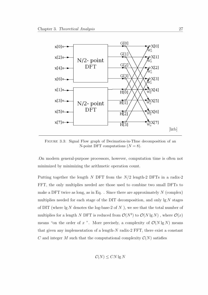
Figure 3.3: Signal Flow graph of Decimation-in-TIme decomposition of anN-point DFT computations (N = 8).
.On modern general-purpose processors, however, computation time is often not
minimized by minimizing the arithmetic operation count.
Putting together the length N DFT from the N/2 length-2 DFTs in a radix-2
FFT, the only multiplies needed are those used to combine two small DFTs to
make a DFT twice as long, as in Eq. . Since there are approximately N (complex)
multiplies needed for each stage of the DIT decomposition, and only lgN stages
of DIT (where lgN denotes the log-base-2 of N ), we see that the total number of
multiplies for a length N DFT is reduced from O(N2) to O(N lgN) , where O(x)
means “on the order of x ”. More precisely, a complexity of O(N lgN) means
that given any implementation of a length-N radix-2 FFT, there exist a constant
C and integer M such that the computational complexity C(N) satisfies
C(N) ≤ CN lgN
Chapter 3. Theoretical Analysis 28
for all N > M . In summary, the complexity of the radix-2 FFT is said to be “N
log N”, or O(N lgN) .
3.3.4 Computational cost of radix-2 DIT FFT
• N2log2N complex multiplies
• Nlog2N complex adds
This is a remarkable savings over direct computation of the DFT. For example,
a length-1024 DFT would require 1048576 complex multiplications and 1047552
complex additions with direct computation, but only 5120 complex multiplications
and 10240 complex additions using the radix-2 FFT, a savings by a factor of 100
or more. The relative savings increase with longer FFT lengths, and are less for
shorter lengths.
Modest additional reductions in computation can be achieved by noting that cer-
tain twiddle factors, namely Using special butterflies forW 0N ,W
N2N ,W
N4N ,W
N8N ,W
3N8
N ,
require no multiplications, or fewer real multiplies than other ones.
3.4 Prime Factor Algorithm (PFA)
By the prime factorization theorem, every integer N can be uniquely factored into
a product of prime numbers pi raised to an integer power mi ≥ 1 :
N =
np∏i=1
pmii
As discussed above, a mixed-radix Cooley Tukey FFT can be used to implement
a length N DFT using DFTs of length pi . However, for factors of N that are
Chapter 3. Theoretical Analysis 29
mutually prime (such as pmii and p
mj
j for i 6= j ), a more efficient prime factor
algorithm (PFA), also called the Good-Thomas FFT algorithm, can be used. The
Chinese Remainder Theorem is used to re-index either the input or output samples
for the PFA.A.5Since the PFA is only applicable to mutually prime factors of N
, it is ideally combined with a mixed-radix Cooley-Tukey FFT, which works for
any integer factors. It is interesting to note that the PFA actually predates the
Cooley-Tukey FFT paper of 1965 [6], with Good’s 1958 work on the PFA being
cited in that paper [16].
The PFA and Winograd transform are closely related, with the PFA being some-
what faster.
3.5 Radix-4 FFT Algorithms
When the number of data points N in the DFT is a power of 4(i.e., N = 4v),we
can, of course, always use a Radix-2 algorithm for computation. However, for this
case, it is more efficient computationally to employ a radix-4 FFT algorithm.[17]
Let us begin by describing a radix-4 decimation-in-time FFT algorithm, which is
obtained by selecting L = 4 and M = N/4 divide-and-conquer-approach for the
choice of L and M, we have l,p = 0, 1, 2, 3; m,q = 0, 1...., N/4−1; n = 4m+l; and k =
(N/4)p+q. Thus we split or determine the N-point input sequence into four sub
sequences, x(4n), x(4n+ 1), x(4n+ 2), x(4n+ 3), n = 0, 1, ......, N/4− 1.
By applying Eq. (??)
X(p, q) =3∑l=0
[W lqNF (l, q)
]W lp
4 , p = 0, 1, 2, 3, 4 (3.24)
where F(l,q) is given by
Chapter 3. Theoretical Analysis 30
F (l, q) =
(N/4)−1∑m=0
x(l,m)WmqN/4, (3.25)
l = 0, 1, 2, 3, q = 01, 2, ...., N4− 1
and
x(l,m) = x(4m+ l) (3.26)
X(p, q) = X(N
4+ q) (3.27)
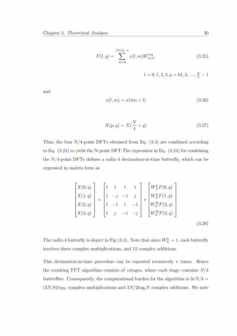
Thus, the four N/4-point DFTs obtained from Eq. (3.4) are combined according
to Eq. (3.24) to yield the N-point DFT.The expression in Eq. (3.24) for combining
the N/4-point DFTs defines a radix-4 decimation-in-time butterfly, which can be
expressed in matrix form as
X(0, q)
X(1, q)
X(2, q)
X(3, q)
=
1 1 1 1
1 −j −1 j
1 −1 1 −1
1 j −1 −j
∗W 0NF (0, q)
W qNF (1, q)
W 2qN F (2, q)
W 3qN F (3, q)
(3.28)
The radix-4 butterfly is depict in Fig (3.4). Note that since W 0N = 1, each butterfly
involves three complex multiplications, and 12 complex additions.
This decimation-in-time procedure can be repeated recursively v times. Hence
the resulting FFT algorithm consists of vstages, where each stage contains N/4
butterflies. Consequently, the computational burden for the algorithm is 3vN/4 =
(3N/8)logN complex multiplications and 3N/2log2N complex additions. We note
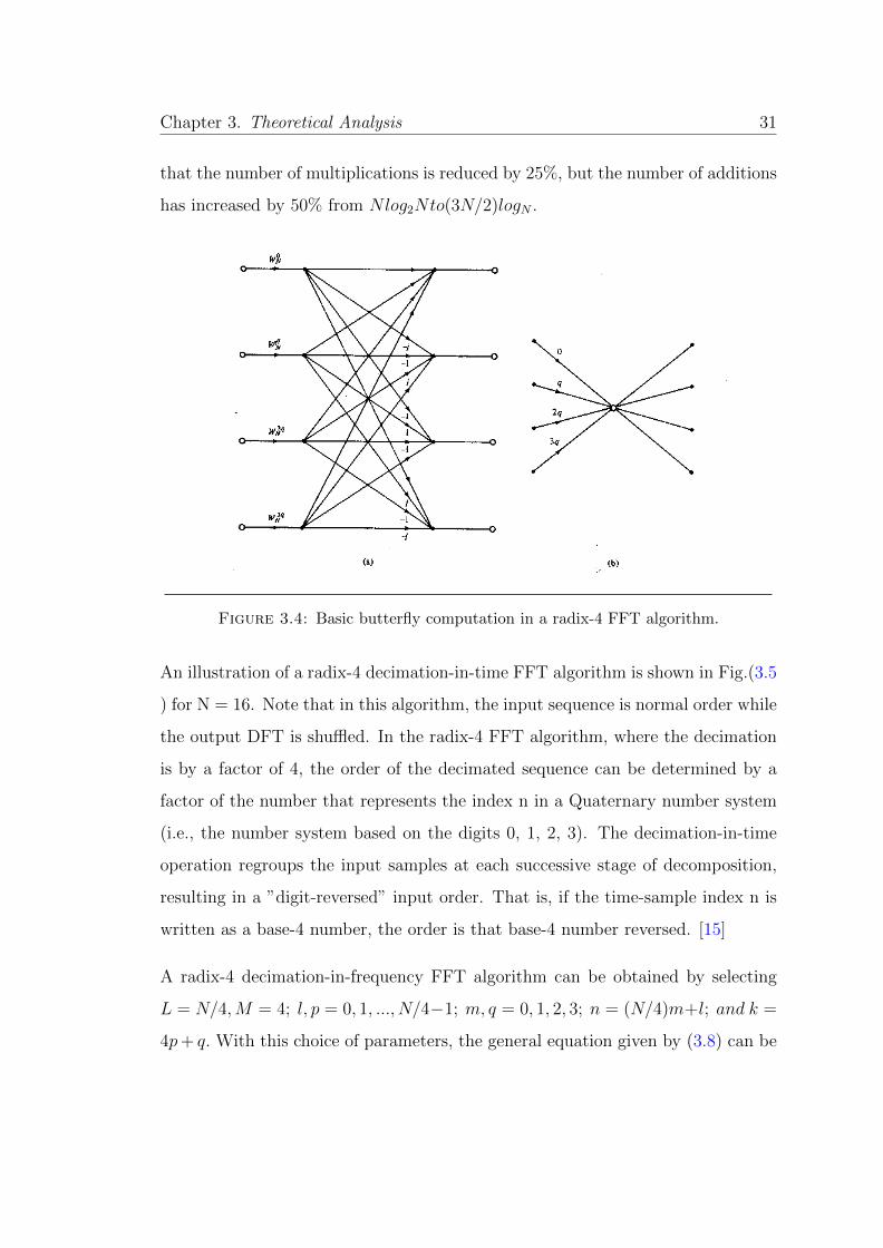
Chapter 3. Theoretical Analysis 31
that the number of multiplications is reduced by 25%, but the number of additions
has increased by 50% from Nlog2Nto(3N/2)logN .
Figure 3.4: Basic butterfly computation in a radix-4 FFT algorithm.
An illustration of a radix-4 decimation-in-time FFT algorithm is shown in Fig.(3.5
) for N = 16. Note that in this algorithm, the input sequence is normal order while
the output DFT is shuffled. In the radix-4 FFT algorithm, where the decimation
is by a factor of 4, the order of the decimated sequence can be determined by a
factor of the number that represents the index n in a Quaternary number system
(i.e., the number system based on the digits 0, 1, 2, 3). The decimation-in-time
operation regroups the input samples at each successive stage of decomposition,
resulting in a ”digit-reversed” input order. That is, if the time-sample index n is
written as a base-4 number, the order is that base-4 number reversed. [15]
A radix-4 decimation-in-frequency FFT algorithm can be obtained by selecting
L = N/4,M = 4; l, p = 0, 1, ..., N/4−1; m, q = 0, 1, 2, 3; n = (N/4)m+l; and k =
4p+ q. With this choice of parameters, the general equation given by (3.8) can be

Chapter 3. Theoretical Analysis 32
Figure 3.5: 16-point radix-4 decimation-in-time algorithm with input in nor-mal order and output in bit reversed order The integer multipliers shown on the
graph represent the exponent on W16.
expressed as
X(p, q) =
(N/4)−1∑l=0
G(l, q)W lpN/4 (3.29)
where
G(l, q) = W lqNF (l, q), (3.30)
q = 0, 1, 2, 3, l = 01, 2, ...., N4− 1
and
F (l, q) =3∑
m=0
x(l,m)Wmq4 , (3.31)
q = 0, 1, 2, 3, l = 01, 2, ...., N4− 1
Chapter 3. Theoretical Analysis 33
For illustrative purposes, let us re-derive the radix-4 decimation-in-frequency al-
gorithm by breaking the N-point DFT formula into four smaller DFTs. We have
X[k] =N−1∑n=0
x[n]W nkN
=
N/4−1∑n=0
x[n]W knN +
N/2−1∑n=N/4
x[n]W knN +
3N/4−1∑n=N/2
x[n]W knN +
N−1∑n=3N/4
x[n]W knN
=
N/4−1∑n=0
x[n]W knN +W
Nk/4N
N/4−1∑n=0
x(n+N
4)W nk
N +WNk/2N
N/4−1∑n=0
x(n+N
2)W nk
N
+ W3Nk/4N
N/4−1∑n=0
x(n+3N
4)W nk
N (3.32)
From the definition of the twiddle factors, we have
WNk/4N = (−j)k,
WNk/2N = (−1)k,
W3Nk/4N = (j)k (3.33)
After substitution of Eq.(3.33) into Eq. (3.32), we obtaion
X(k) =
N/4−1∑n=0
[x(n) + (−j)kx(n+
N
4) + (−1)kx(n+
N
2) + (j)kx(n+
3N
4)
]W nkN
(3.34)
The relation is not an N/4-point DFT because the twiddle factor depends on N and
not on N/4. To convert it into an N/4-point DFT, we subdivide the DFT sequence
Chapter 3. Theoretical Analysis 34
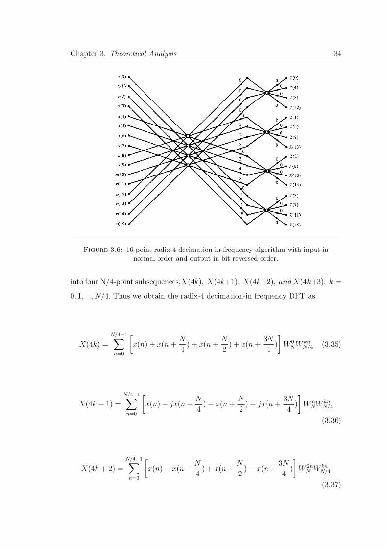
Figure 3.6: 16-point radix-4 decimation-in-frequency algorithm with input innormal order and output in bit reversed order.
into four N/4-point subsequences,X(4k), X(4k+1), X(4k+2), and X(4k+3), k =
0, 1, ..., N/4. Thus we obtain the radix-4 decimation-in frequency DFT as
X(4k) =
N/4−1∑n=0
[x(n) + x(n+
N
4) + x(n+
N
2) + x(n+
3N
4)
]W 0NW
knN/4 (3.35)
X(4k + 1) =
N/4−1∑n=0
[x(n)− jx(n+
N
4)− x(n+
N
2) + jx(n+
3N
4)
]W nNW
knN/4
(3.36)
X(4k + 2) =
N/4−1∑n=0
[x(n)− x(n+
N
4) + x(n+
N
2)− x(n+
3N
4)
]W 2nN W kn
N/4
(3.37)

Chapter 3. Theoretical Analysis 35
X(4k + 3) =
N/4−1∑n=0
[x(n) + jx(n+
N
4)− x(n+
N
2)− jx(n+
3N
4)
]W 3nN W kn
N/4
(3.38)
where we have used the property W 4knN = W kn
N/4. Note that the input to each
N/4-point DFT is a linear combination of four signal samples scaled by a twiddle
factor. This procedure is repeated v times, where v = log4N.
3.5.1 Radix-4 FFT Operation Counts
• 3N4log2N
2= 3
8Nlog2Ncomplex multiplies (75% of a radix-2 FFT)
• 8N4log2N
2= Nlog2N complex adds (same as a radix-2 FFT)
The radix-4 FFT requires only 75% as many complex multiplies as the radix-2
FFTs, although it uses the same number of complex additions. These additional
savings make it a widely-used FFT algorithm.
Chapter 4
Experimental Investigations
4.1 Understanding the FFT
FFT algorithms are based on the fundamental principle of decomposing the com-
putation of the discrete Fourier Transform of a sequence of length N into succes-
sively smaller discrete Fourier transform. The manner in which the principle is
implemented leads to a variety of different algorithms, all with comparable im-
provements in computational speed.
The DFT is inefficient and takes a lot of computational time for larger number of
N compare to FFT, because it does not exploit the properties stated in Eq. (3.10)
& (3.11). To understand FFT in depth we need to understand the phase factors
and its properties first.
4.1.1 Phase factors / Twiddle factors
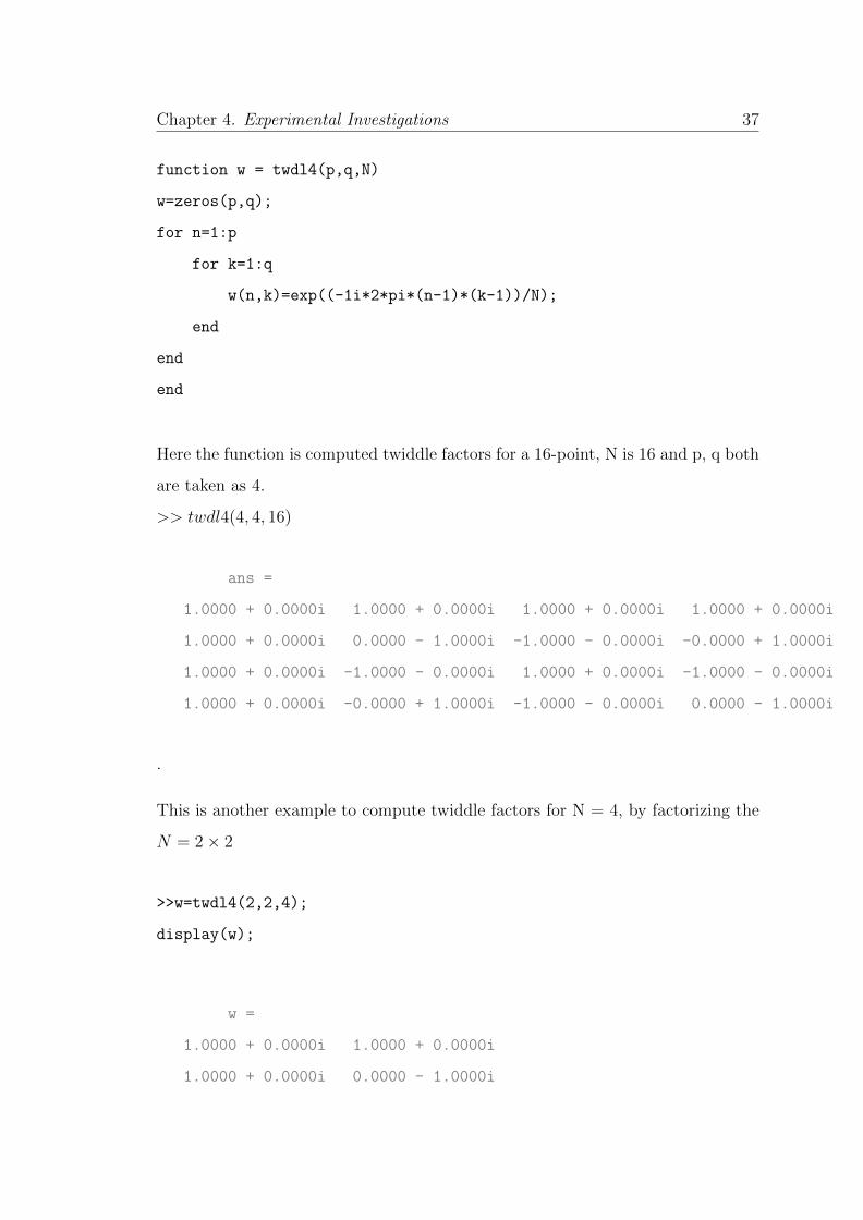
The following function will compute the twiddle factors for an N-point sequence
by its composite factors. Therefore N = pq;
36
Chapter 4. Experimental Investigations 37
function w = twdl4(p,q,N)
w=zeros(p,q);
for n=1:p
for k=1:q
w(n,k)=exp((-1i*2*pi*(n-1)*(k-1))/N);
end
end
end
Here the function is computed twiddle factors for a 16-point, N is 16 and p, q both
are taken as 4.
>> twdl4(4, 4, 16)
ans =
1.0000 + 0.0000i 1.0000 + 0.0000i 1.0000 + 0.0000i 1.0000 + 0.0000i
1.0000 + 0.0000i 0.0000 - 1.0000i -1.0000 - 0.0000i -0.0000 + 1.0000i
1.0000 + 0.0000i -1.0000 - 0.0000i 1.0000 + 0.0000i -1.0000 - 0.0000i
1.0000 + 0.0000i -0.0000 + 1.0000i -1.0000 - 0.0000i 0.0000 - 1.0000i
.
This is another example to compute twiddle factors for N = 4, by factorizing the
N = 2× 2
>>w=twdl4(2,2,4);
display(w);
w =
1.0000 + 0.0000i 1.0000 + 0.0000i
1.0000 + 0.0000i 0.0000 - 1.0000i
Chapter 4. Experimental Investigations 38
These phase factors can be used to compute FFT for a 4-point sequence.
Similarly we can generate the phase factors with respect to the decomposition of
N.(4.1.1)
4.1.2 Multi-Dimensional Index Mapping
Index mapping is a technique to reduce the required arithmetic to compute DFT
of a N-point input[18].
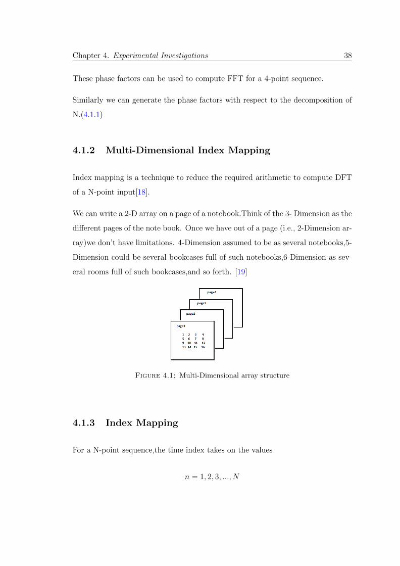
We can write a 2-D array on a page of a notebook.Think of the 3- Dimension as the
different pages of the note book. Once we have out of a page (i.e., 2-Dimension ar-
ray)we don’t have limitations. 4-Dimension assumed to be as several notebooks,5-
Dimension could be several bookcases full of such notebooks,6-Dimension as sev-
eral rooms full of such bookcases,and so forth. [19]
Figure 4.1: Multi-Dimensional array structure
4.1.3 Index Mapping
For a N-point sequence,the time index takes on the values
n = 1, 2, 3, ..., N
Chapter 4. Experimental Investigations 39
where N=4v, so that the index mapping for the N-point of 1-dimensional array to
v -dimensional array is given by
n =N
41n1 +
N
42n2 + ...+
N
4v−1nv−1 +
N
4vnv
where n1, n2, n3...nv =0,1,2,3
similarly k is also mapped from 1-dimensional array to v -dimensional array as
k =N
4vk1 +
N
4v−1k2 + ...+
N
42kv−1 +
N
41kv
Therefore equation (3.8) can be written as
X
[k1 + 4k2 + ...+ 4vkv
]
=3∑
nv=0
3∑nv−1=0
...3∑
n1=0
x
(N
4n1 +
N
42n2+
...+N
4vnv)
)WN
(N4n1+
N42n2+...+
N4vnv)∗(k1+4k2+...+4vkv) (4.1)
Note : The number 4 in the denominator of the above Equations can be replaced
with ”r”, where r is the radix of your interest.
4.2 Radix-42 FFT/IFFT Algorithm
For N=16 (i.e., N=42), To perform index mapping on the 16-point input, Equation
(4.1) can be recast as
X[k1 + 4k2]
=3∑
n2=0
3∑n1=0
x(4n1 + n2)W16(4n1+n2)∗(k1+4k2) (4.2)

Chapter 4. Experimental Investigations 40
here the twiddle factor W16(4n1+n2)∗(k1+4k2) can be decomposed as[20]
= W164n1k1 .W16
16n1k2 .W16n1k2 .W16
4n2k2
where W1616n1k2 = 1,Therefore Equation (4.2) can be recast as
X[k1 + 4k2]
=3∑
n2=0
[3∑
n1=0
x(4n1 + n2)W4n1k1
].W16
n1k2
.W4
n2k2 (4.3)
here W4n1k1 ,W4
4n2k2 are DFT kernels and both are equal.and W16n1k2
are the twiddle factors,the complex multiplications required are
W k116 , (W
−k116 ),W 2k1
16 , (W−2k116 ),W 3k1
16 , (W−3k116 ) in the N-point FFT/IFFT mode.
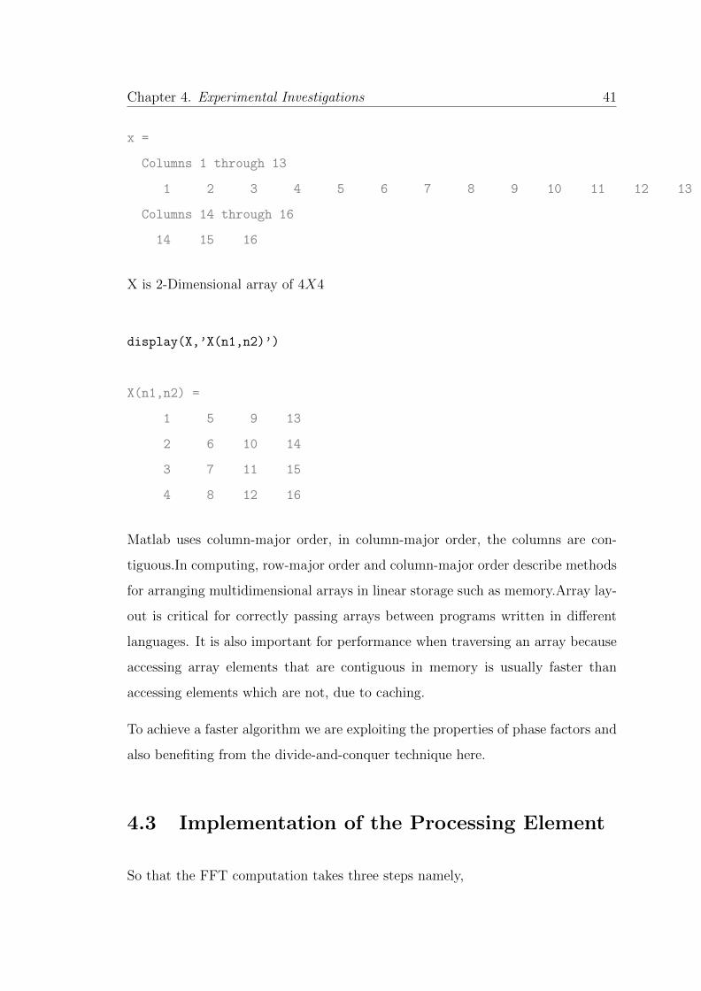
16-point Index Map
Considering an N-point sequence, where N = 16, and decomposing it into 4 x 4.
x(n) is one-dimensional array
x=1:16;
display(x)
for n1=1:4
for n2=1:4
X(n1,n2)=x(4*(n1-1)+n2);
end
end
X=X’;
Chapter 4. Experimental Investigations 41
x =
Columns 1 through 13
1 2 3 4 5 6 7 8 9 10 11 12 13
Columns 14 through 16
14 15 16
X is 2-Dimensional array of 4X4
display(X,’X(n1,n2)’)
X(n1,n2) =
1 5 9 13
2 6 10 14
3 7 11 15
4 8 12 16
Matlab uses column-major order, in column-major order, the columns are con-
tiguous.In computing, row-major order and column-major order describe methods
for arranging multidimensional arrays in linear storage such as memory.Array lay-
out is critical for correctly passing arrays between programs written in different
languages. It is also important for performance when traversing an array because
accessing array elements that are contiguous in memory is usually faster than
accessing elements which are not, due to caching.
To achieve a faster algorithm we are exploiting the properties of phase factors and
also benefiting from the divide-and-conquer technique here.
4.3 Implementation of the Processing Element
So that the FFT computation takes three steps namely,
Chapter 4. Experimental Investigations 42
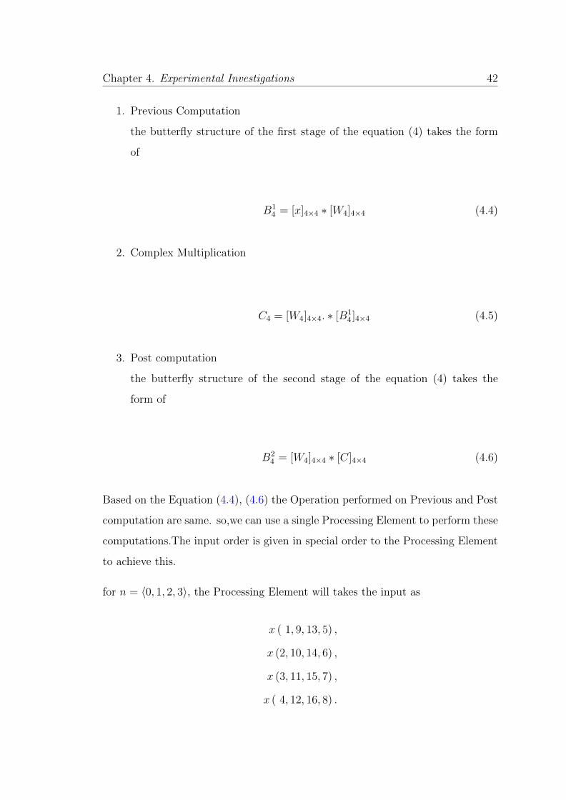
1. Previous Computation
the butterfly structure of the first stage of the equation (4) takes the form
of
B14 = [x]4×4 ∗ [W4]4×4 (4.4)
2. Complex Multiplication
C4 = [W4]4×4. ∗ [B14 ]4×4 (4.5)
3. Post computation
the butterfly structure of the second stage of the equation (4) takes the
form of
B24 = [W4]4×4 ∗ [C]4×4 (4.6)
Based on the Equation (4.4), (4.6) the Operation performed on Previous and Post
computation are same. so,we can use a single Processing Element to perform these
computations.The input order is given in special order to the Processing Element
to achieve this.
for n = 〈0, 1, 2, 3〉, the Processing Element will takes the input as
x ( 1, 9, 13, 5) ,
x (2, 10, 14, 6) ,
x (3, 11, 15, 7) ,
x ( 4, 12, 16, 8) .
Chapter 4. Experimental Investigations 43
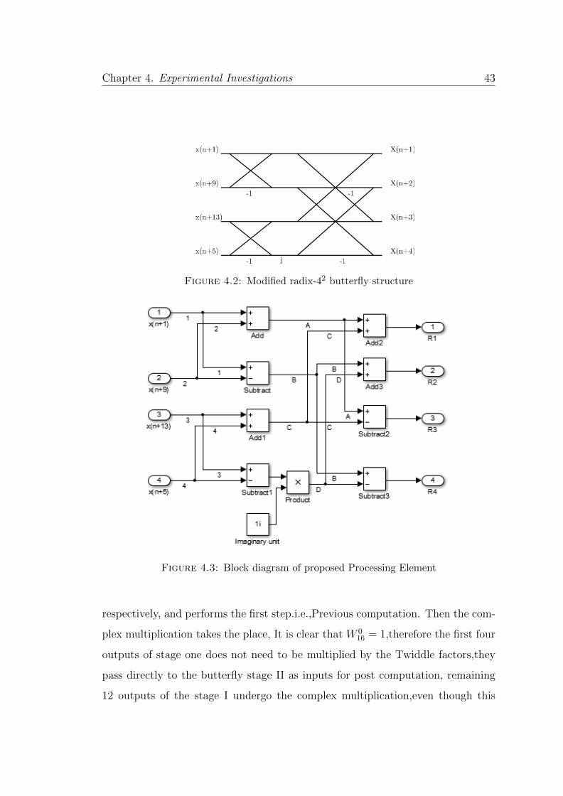
Figure 4.2: Modified radix-42 butterfly structure
Figure 4.3: Block diagram of proposed Processing Element
respectively, and performs the first step.i.e.,Previous computation. Then the com-
plex multiplication takes the place, It is clear that W 016 = 1,therefore the first four
outputs of stage one does not need to be multiplied by the Twiddle factors,they
pass directly to the butterfly stage II as inputs for post computation, remaining
12 outputs of the stage I undergo the complex multiplication,even though this

Chapter 4. Experimental Investigations 44
complex multiplication can be further reduced to 9 by using the same property
W 016 = 1 and produce intermediate results for post computation as
R1 ( 1, 2, 3, 4) ,
R2 ( 5, 6, 7, 8) ,
R3 ( 9, 10, 11, 12) ,
R4 (13, 14, 15, 16) .
now to compute the final result,these intermediate results are given input to the
Processing Element in the following order
R1 (1, 9, 13, 5) ,
R2 (2, 10, 14, 6) ,
R3 (3, 11, 15, 7) ,
R4 (4, 12, 16, 8) .
for 〈n = 0, 1, 2, 3〉, the PE computes R1,R2,R3,R4 respectively and produces the
output
X ( 1, 9, 13, 5) ,
X (2, 10, 14, 6) ,
X (3, 11, 15, 7) ,
X ( 4, 12, 16, 8) .
The Final Output is obtained by applying index mapping on X. i.e.,X [k1 + 4k2]
for 〈k1, k2 = 0, 1, 2, 3〉, in other words the [X]4×4 is to be transposed.

Chapter 4. Experimental Investigations 45
Similarly we can perform index mapping on any number of N-point (N=4v i.e.,
N=16,64,256,1024,4096,...) 1-Dimensional array.[21]
However we can achieve Inverse Fast Fourier Transform (IFFT) with a little mod-
ification to the FFT algorithm,i.e., sign inversion on the twiddle factors and Nor-
malizing by dividing N .Therefore IFFT formula is given by
x[4n1 + n2]
=1
N
3∑k2=0
3∑k1=0
X(k1 + 4k2)W16−(4n1+n2)∗(k1+4k2) (4.7)
x[4n1 + n2]
=1
N
3∑k2=0
[3∑
k1=0
X(k1 + 4k2)W4−n1k1
].W16
−n1k2
.W4
−n2k2 (4.8)
4.4 FFT Design Using Simulink
4.4.1 Simulink
Simulink R© is a block diagram environment for multidomain simulation and Model-
Based Design. It supports simulation, automatic code generation, and continuous
test and verification of embedded systems.
Simulink provides a graphical editor, customizable block libraries, and solvers for
modeling and simulating dynamic systems. It is integrated with MATLAB R©, en-
abling you to incorporate MATLAB algorithms into models and export simulation
results to MATLAB for further analysis. Simulink is widely used in control theory
and digital signal processing for multidomain simulation and Model-Based Design.
Chapter 4. Experimental Investigations 46
HDL CoderTM generates portable, synthesizable Verilog R© and VHDL R© code from
MATLAB R© functions, Simulink R©models, and Stateflow R© charts. The generated
HDL code can be used for FPGA programming or ASIC prototyping and design.
HDL Coder provides a workflow advisor that automates the programming of
Xilinx R© and Altera R© FPGAs. You can control HDL architecture and imple-
mentation, highlight critical paths, and generate hardware resource utilization es-
timates. HDL Coder provides traceability between your Simulink model and the
generated Verilog and VHDL code, enabling code verification for high-integrity
applications adhering to DO-254 and other standards.
4.4.2 Generating HDL Code
HDL Coder lets you generate synthesizable HDL code for FPGA and ASIC im-
plementations in a few steps:
Model your design using a combination of MATLAB code, Simulink blocks, and
Stateflow charts. Optimize models to meet area-speed design objectives. Gen-
erate HDL code using the integrated HDL Workflow Advisor for MATLAB and
Simulink. Verify generated code using HDL VerifierTM.
4.4.3 HDL Code Generation from MATLAB
The HDL Workflow Advisor in HDL Coder automatically converts MATLAB code
from floating-point to fixed-point and generates synthesizable VHDL and Verilog
code. This capability lets you model your algorithm at a high level using abstract
MATLAB constructs and System objects while providing options for generating
HDL code that is optimized for hardware implementation. HDL Coder provides
a library of ready-to-use logic elements, such as counters and timers, which are
written in MATLAB.
Chapter 4. Experimental Investigations 47
4.4.4 HDL Code Generation from Simulink
The HDL Workflow Advisor Fig.4.9 generates VHDL and Verilog code from
Simulink and Stateflow. With Simulink, you can model your algorithm using
a library of more than 200 blocks, including Stateflow charts. This library pro-
vides complex functions, such as the Viterbi decoder, FFT, CIC filters, and FIR
filters, for modeling signal processing and communications systems and generating
HDL code.
4.4.5 Model Designing
Hardware can be Implement for Mathematical models by using Mathwork’s
Simulink.In Simulink library we will find most of all sorts of industry hardware
models to model and simulate the your design. HDL library in simulink will be
very useful to generate hardware for the model designed. To open Simulink library
using command window type
simulink
My Algorithm has been Implemented Using hdllib.
The main root system consists of three stages, which are described in detailed in
the section 4.3. Stage 1 Fig.4.5 and Stage 3 Fig.4.7 consists of Processing Element
Fig.4.5, and the second stage only consists of multiplications Fig.4.7.
Blocks Used to Model
1. ADD / SUBTRACT:
The Sum block performs addition or subtraction on its inputs. This block
can add or subtract scalar, vector, or matrix inputs. It can also collapse the
elements of a signal.

Chapter 4. Experimental Investigations 48
Figure 4.4: MATLAB HDL Project : Simulink Model of Radix - 4 FFT
Figure 4.5: MATLAB HDL Project - Processing Element
2. PRODUCT:
By default, the Product block outputs the result of multiplying two inputs:
two scalars, a scalar and a nonscalar, or two nonscalars that have the same
dimensions. The default parameter values that specify this behavior are:
• Multiplication: Element-wise(.*)
Chapter 4. Experimental Investigations 49
• Number of inputs: 2
3. Multiport Selector: The Multiport Selector block extracts multiple sub-
sets of rows or columns from M-by-N input matrix u, and propagates each
new submatrix to a distinct output port. The block treats an unoriented
length-M vector input as an M-by-1 matrix.
The Indices to output parameter is a cell array whose kth cell contains a
one-dimensional indexing expression specifying the subset of input rows or
columns to be propagated to the kth output port. The total number of cells
in the array determines the number of output ports on the block.
When you set the Select parameter to Rows, the block uses the one-
dimensional indices you specify to select matrix rows, and all elements
on the chosen rows are included. When you set the Select parameter to
Columns, the block uses the one-dimensional indices you specify to select
matrix columns, and all elements on the chosen columns are included. A
given input row or column can appear any number of times in any of the
outputs, or not at all.
When an index references a nonexistent row or column of the input, the
block reacts with the action you specify using the Invalid index parameter.
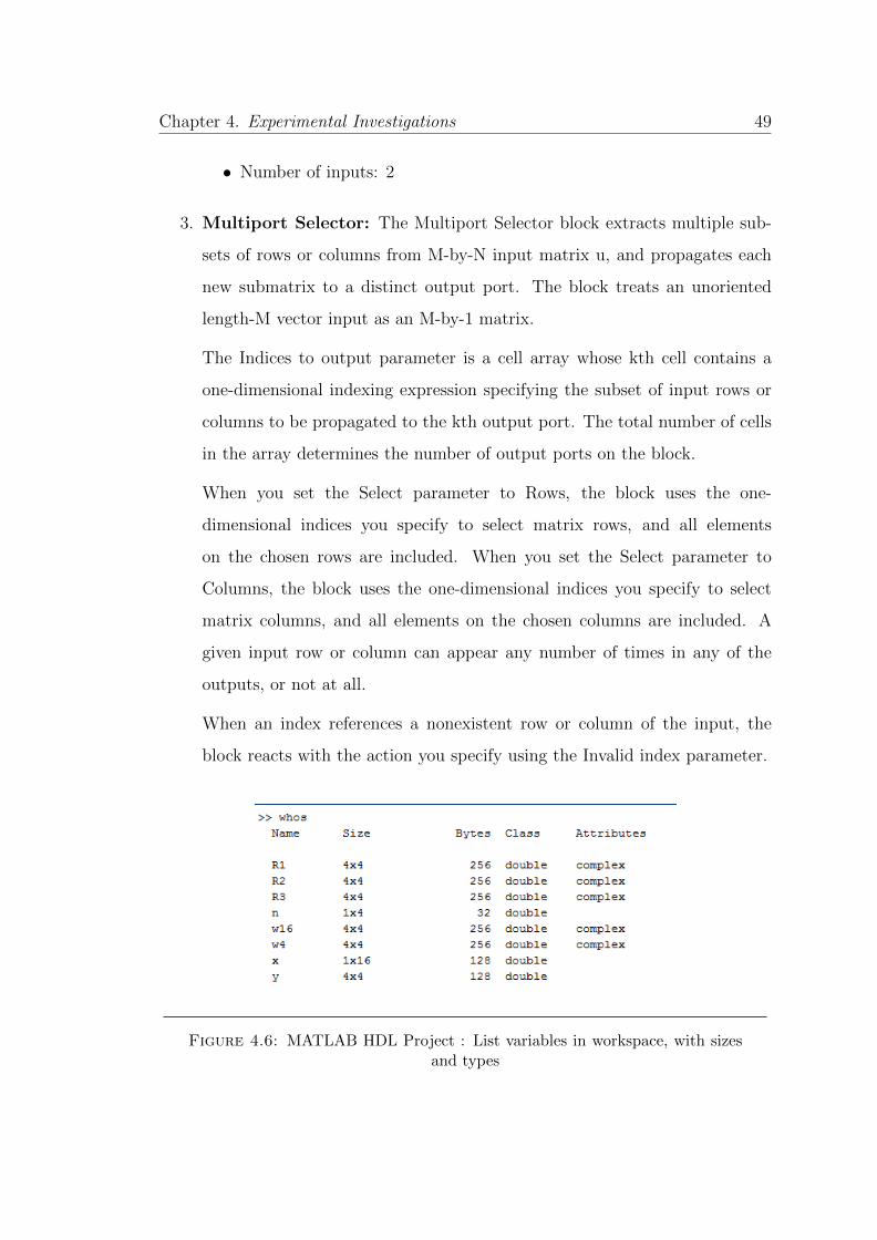
Figure 4.6: MATLAB HDL Project : List variables in workspace, with sizesand types

Chapter 4. Experimental Investigations 50
This will takes the input from the work space here. List variables in workspace,
with sizes and types as shown in Fig. 4.6.
Figure 4.7: MATLAB HDL Project : Second Stage
In the second stage the multiplication is performed using twiddle factors.
Column 1 Column 2 Column 3 Coulmn 41 1 1 11 0.9239 - 0.3827i 0.7071 - 0.7071i 0.3827 - 0.9239i1 0.7071 - 0.7071i 0.0000 - 1.0000i -0.7071 - 0.7071i1 0.3827 - 0.9239i -0.7071 - 0.7071i -0.9239 + 0.3827i
Table 4.1: Twiddle Factors : W16
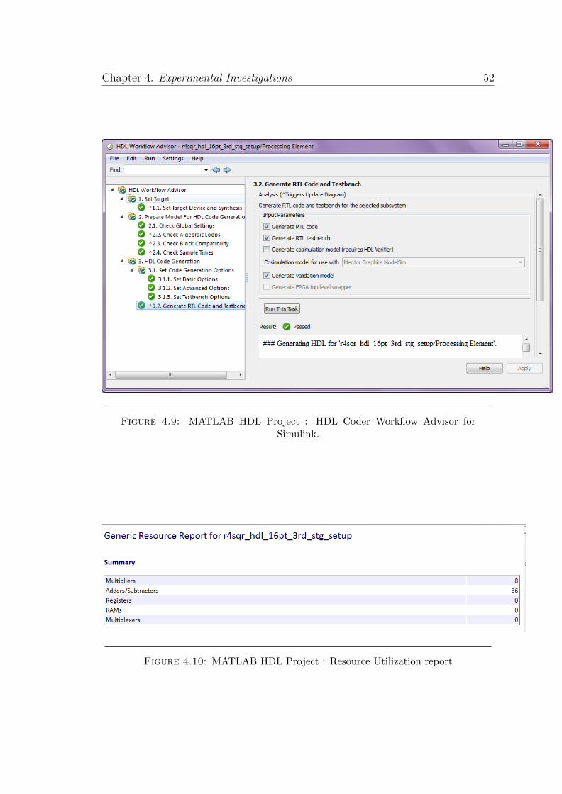
HDL Coder workflow advicer Fig.4.9 is used to generate HDL code for the designed
model. it passed all the checks and generated report all that specified.
Chapter 4. Experimental Investigations 51
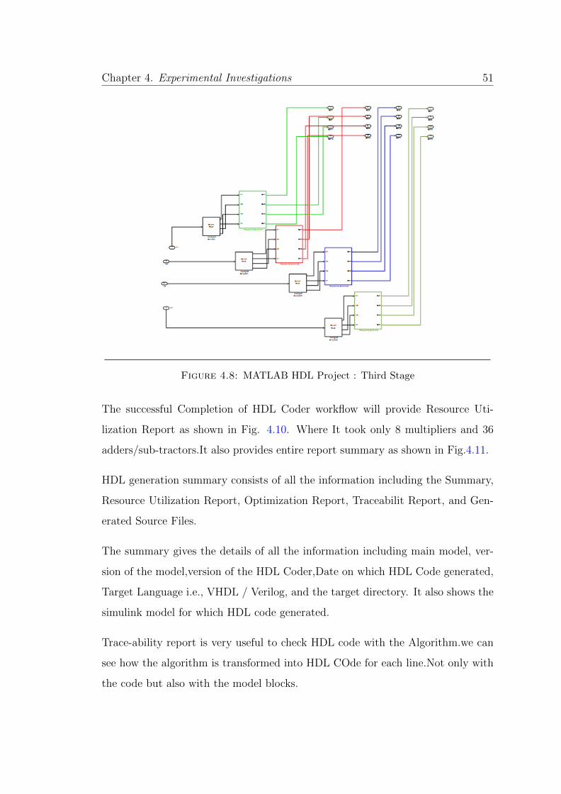
Figure 4.8: MATLAB HDL Project : Third Stage
The successful Completion of HDL Coder workflow will provide Resource Uti-
lization Report as shown in Fig. 4.10. Where It took only 8 multipliers and 36
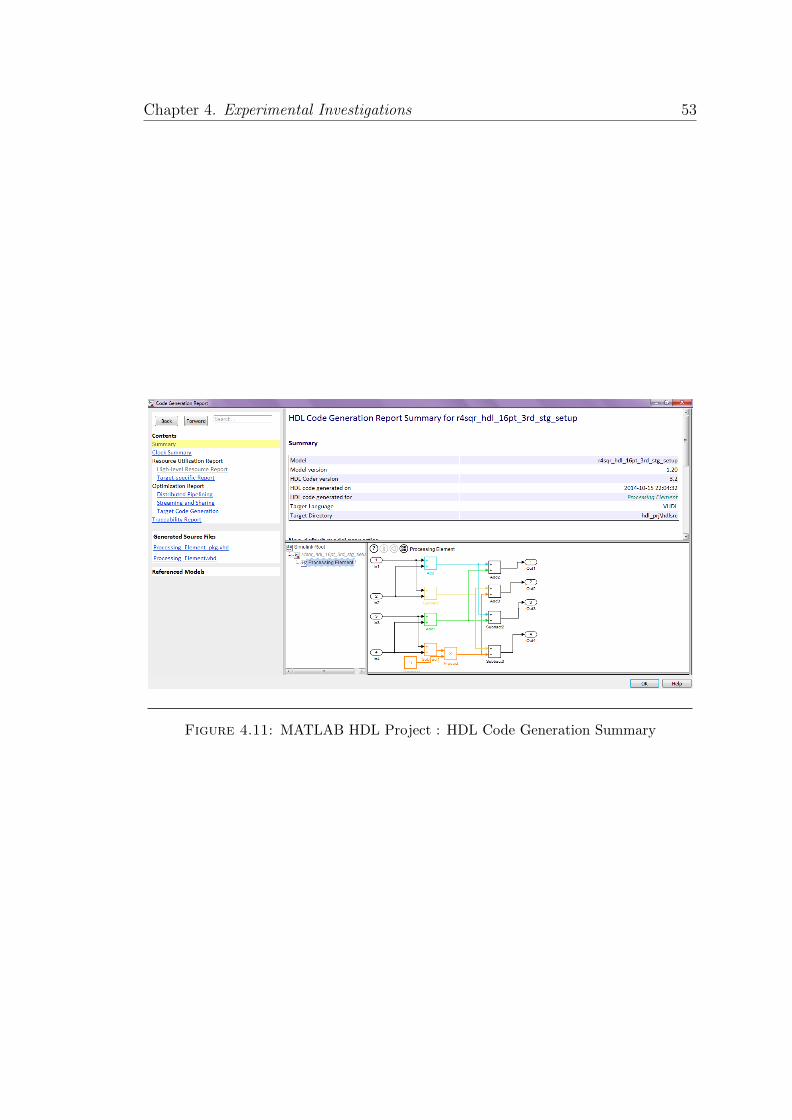
adders/sub-tractors.It also provides entire report summary as shown in Fig.4.11.
HDL generation summary consists of all the information including the Summary,
Resource Utilization Report, Optimization Report, Traceabilit Report, and Gen-
erated Source Files.
The summary gives the details of all the information including main model, ver-
sion of the model,version of the HDL Coder,Date on which HDL Code generated,
Target Language i.e., VHDL / Verilog, and the target directory. It also shows the
simulink model for which HDL code generated.
Trace-ability report is very useful to check HDL code with the Algorithm.we can
see how the algorithm is transformed into HDL COde for each line.Not only with
the code but also with the model blocks.
Chapter 4. Experimental Investigations 52
Figure 4.9: MATLAB HDL Project : HDL Coder Workflow Advisor forSimulink.
Figure 4.10: MATLAB HDL Project : Resource Utilization report
Chapter 4. Experimental Investigations 53
Figure 4.11: MATLAB HDL Project : HDL Code Generation Summary
Chapter 5
Experimental Results
5.1 Prototyping as C/C++ Code
So far we have developed MATLAB R© programs and Simulink models in order to
simulate the FFT / IFFT models in the MATLAB environment. At some stage
in the work flow of a communications system design, we might need to produce
a software component that cannot be directly simulated in MATLAB. For exam-
ple, we might need to interface to an existing simulation environment based on
a C/C++ software implementation. If we want to export the result of modeling
and simulation in MATLAB to an external C/C++ programming environment,
we essentially have two choices: we can either manually translate algorithms de-
veloped in MATLAB into a C or C++ implementation or we can take advantage
of automatic MATLAB C-code generation. By using MATLAB Coder, we can
generate standalone C and C++ code from MATLAB code. The generated source
code is portable and readable. MATLAB Coder supports a subset of MATLAB
language features, including program control constructs, functions, and matrix
operations. It can generate MATLAB executable (MEX) functions that let us
54
Chapter 5. Experimental Results 55
accelerate computationally intensive portions of MATLAB code and verify its be-
havior. It can also generate C/C++ source code for integration with existing C
code, creation of an executable prototype, or direct implementation on a Digital
Signal Processor (DSP) or general-purpose CPU using a C/C++ compiler. In this
chapter we examine the process of generating standalone C and C++ code from
MATLAB code using MATLAB Coder. We first present use cases, motivations,
and requirements for C/C++ code generation and then examine the mechanics
of code generation using two methods: (i) calling code-generation functions from
the MATLAB command line and (ii) using the MATLAB Coder Project Applica-
tion. We then elaborate on the extent of support for code generation inMATLAB,
highlighting code-generation support by various System toolboxes and support for
various data types, including fixed-point data, and forMATLAB programs em-
ploying variable-sized data. Finally, we present a full workflow for the integration
of generated code from a MATLAB algorithm into an existing C/C++ testbench.
5.1.1 Use Cases
Before we tackle the subject of generating C code from MATLAB, let us first
elucidate the reasons why engineers translate MATLAB code to C today:
• Integration: We may want to integrate our MATLAB algorithms into an
existing C-based project or software, such as a custom simulator, as source
code or libraries.
• Prototyping: We may need to create a standalone prototype or executable
for testing purposes or in order to create proof-of concept demonstrations.
• Acceleration: We may want to wrap the C code as MEX files for execution
back in MATLAB. This use case is essentially for accelerating the execution
of portions of algorithms that are numerically intensive.
Chapter 5. Experimental Results 56
• Implementation:Wemay need to take the C code and implement it in em-
bedded processors as part of a larger system design.
5.1.2 Motivations
With the automatic translation of an algorithm from MATLAB to C, we can
save the time it takes to rewrite the program and debug the low-level C code.
This can provide more time for development and tuning of our algorithms at a
high level in MATLAB. As we update each version of our MATLAB code, we
can then generate a MEX file automatically. We can use the MEX file and call
it in MATLAB in order to verify that the compiled version of the code executes
properly. The MEX file can also be used to speed up the code in most cases.
We can also generate source code, executables, or libraries automatically. As a
result, we can maintain one design in MATLAB and periodically get a C/C++
code as a byproduct. Having a single software reference in MATLAB makes it
easier to make changes or to improve the performance. As will be discussed in this
chapter, we can also leverage automated tools to help assess the readiness of the
MATLAB code for code generation. These tools can guide us in the steps needed
to successfully generate C code from MATLAB algorithms.
5.1.3 Requirements
In order to generate C/C++ code fromMATLAB algorithms, we must installMAT-
LAB Coder and use a C/C++ compiler. First, we set up the compiler. For most
platforms,MathWorks supplies a default compiler with MATLAB. If an installa-
tion does not include a default compiler, we must obtain and install a supported
C/C++ compiler. The MATLAB documentation contains a list of supported com-
pilers by platform . To set up an installed compiler, at the MATLAB command
line enter:
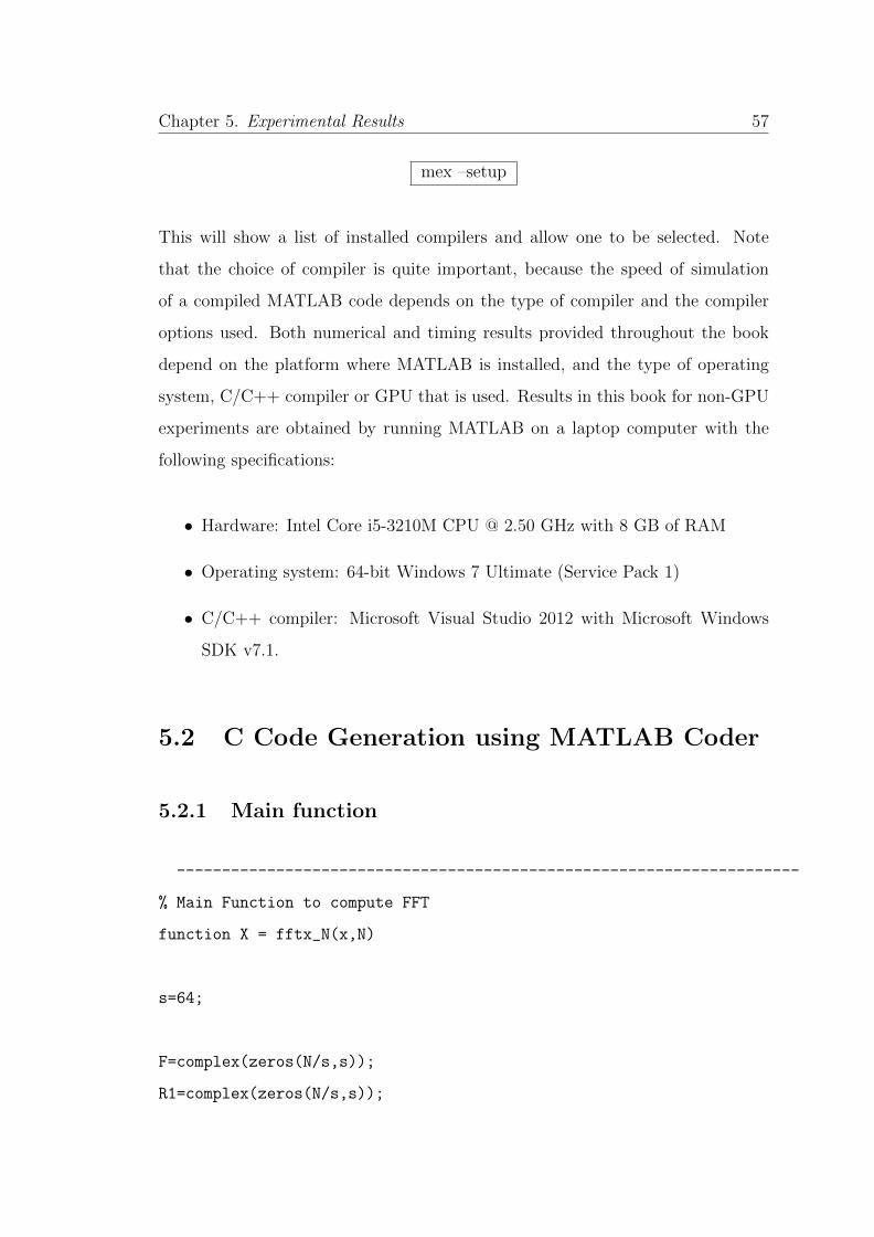
Chapter 5. Experimental Results 57
mex –setup
This will show a list of installed compilers and allow one to be selected. Note
that the choice of compiler is quite important, because the speed of simulation
of a compiled MATLAB code depends on the type of compiler and the compiler
options used. Both numerical and timing results provided throughout the book
depend on the platform where MATLAB is installed, and the type of operating
system, C/C++ compiler or GPU that is used. Results in this book for non-GPU
experiments are obtained by running MATLAB on a laptop computer with the
following specifications:
• Hardware: Intel Core i5-3210M CPU @ 2.50 GHz with 8 GB of RAM
• Operating system: 64-bit Windows 7 Ultimate (Service Pack 1)
• C/C++ compiler: Microsoft Visual Studio 2012 with Microsoft Windows
SDK v7.1.
5.2 C Code Generation using MATLAB Coder
5.2.1 Main function
---------------------------------------------------------------------
% Main Function to compute FFT
function X = fftx_N(x,N)
s=64;
F=complex(zeros(N/s,s));
R1=complex(zeros(N/s,s));
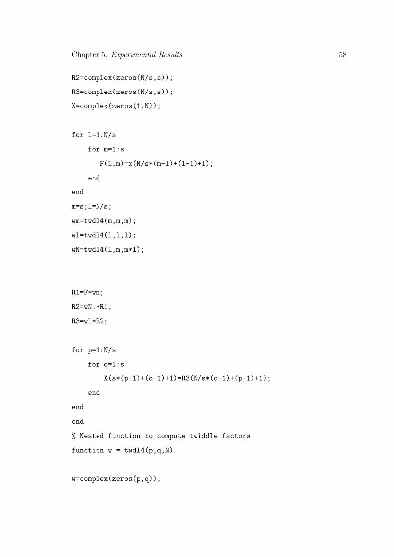
Chapter 5. Experimental Results 58
R2=complex(zeros(N/s,s));
R3=complex(zeros(N/s,s));
X=complex(zeros(1,N));
for l=1:N/s
for m=1:s
F(l,m)=x(N/s*(m-1)+(l-1)+1);
end
end
m=s;l=N/s;
wm=twdl4(m,m,m);
wl=twdl4(l,l,l);
wN=twdl4(l,m,m*l);
R1=F*wm;
R2=wN.*R1;
R3=wl*R2;
for p=1:N/s
for q=1:s
X(s*(p-1)+(q-1)+1)=R3(N/s*(q-1)+(p-1)+1);
end
end
end
% Nested function to compute twiddle factors
function w = twdl4(p,q,N)
w=complex(zeros(p,q));

Chapter 5. Experimental Results 59
for n=1:p
for k=1:q
w(n,k)=exp((-1i*2*pi*(n-1)*(k-1))/N);
end
end
end
---------------------------------------------------------------------
This Function will compute the N-point FFT for the given input sequence x.
To speed up the computation we have pre-allocated some of the variables in the
function with zeros.Fig.5.1 shows the Code Generation Readiness of this function.
To set up your coder environment in MATLAB, in Command Window
coder
Fig.5.2 will appears on the screen, then we need to provide a name and make sure
the output type is MEX, C/C++.
Figure 5.1: MATLABCode Project:CheckingCode Generation Readi-
ness
Figure 5.2: MATLABCode Project:Starting a
new Project
The function is added to the MATLAB Coder as Shown in Fig.5.4. The Function
fftx N is added and we need to define the variable size to each variable in the
function. Here Our variables are x, N. x is defined as double(1 × 256) and N is
defined as constant(double(1× 1)).
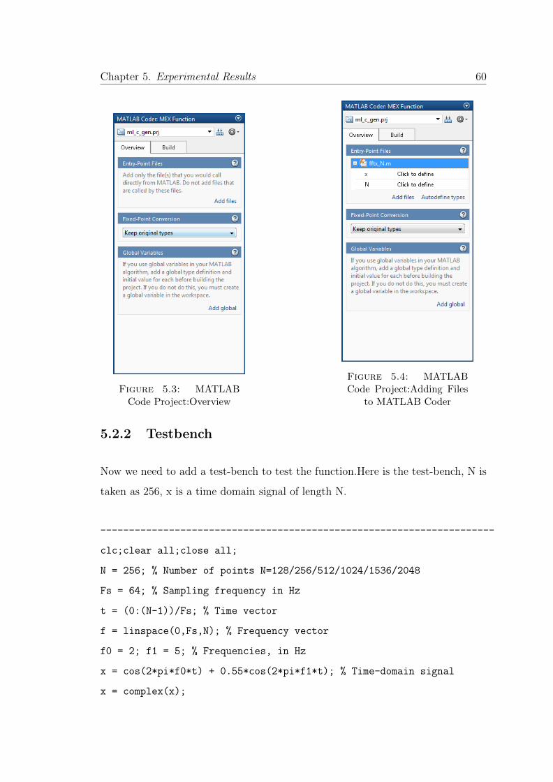
Chapter 5. Experimental Results 60
Figure 5.3: MATLABCode Project:Overview
Figure 5.4: MATLABCode Project:Adding Files
to MATLAB Coder
5.2.2 Testbench
Now we need to add a test-bench to test the function.Here is the test-bench, N is
taken as 256, x is a time domain signal of length N.
---------------------------------------------------------------------
clc;clear all;close all;
N = 256; % Number of points N=128/256/512/1024/1536/2048
Fs = 64; % Sampling frequency in Hz
t = (0:(N-1))/Fs; % Time vector
f = linspace(0,Fs,N); % Frequency vector
f0 = 2; f1 = 5; % Frequencies, in Hz
x = cos(2*pi*f0*t) + 0.55*cos(2*pi*f1*t); % Time-domain signal
x = complex(x);

Chapter 5. Experimental Results 61
X=fftx_N_mex(x,N);
figure(gcf); clf
subplot(211); stem(t,real(x),’b.-’); xlabel(’Time (s)’);
ylabel(’Amplitude’);legend(’X’)
grid on
subplot(212); plot(f,abs(X),’m.-’); xlabel(’Frequency (Hz)’);
ylabel(’Magnitude’);legend(’abs(fft(X))’)
grid on
---------------------------------------------------------------------
Figure 5.5: MATLABCode Project:Defining the
Variables
Figure 5.6: MATLABCode Project:Running for
MEX

Chapter 5. Experimental Results 62
5.2.3 Running MEX and Code Generation
When we click on the Run button, the testbench executes. This enables MATLAB
Coder to infer the size, data type, and complexity of each input variable of the
MATLAB entry-point function. By clicking on the Use These Types button, we
accept these properties and assign them to the input function parameters. As a
last step, we click on the Build tab to select the output file name and output type
and then click on the Build button to generate code Fig.5.9. By default, the output
type is a MEX function. This means that following code generation, MATLAB
Coder compiles the code as a MEX function that can only be called from within
MATLAB environment. The Verification section in theMATLAB Coder Project
enables the generated MEX function to be run with the same testbench (calling
script) used to define the data types. By comparing the result of running the
fftx N.m function with the result of running the MEX function, we can verify that
the MATLAB function and the generated MEX function are numerically identical.
We can obtain the actual C source code generated by MATLAB Coder by changing
the output type to either dynamic C/C++ library or static C/C++ library. In
this example, we just change the output type of the project to static C/C++
library and click on the Build button, as shown in Fig5.7
After the Build button is pressed, the code-generation Build dialog appears Fig.5.9.
As illustrated in the figure, this dialog shows the code-generation progress and
illustrates any error or warning messages that might be generated during the code-
generation process. If code generation is successful, we can click on a hyperlink
that will open the Code Generation Report and show the result of code generation.
In this example, the Code Generation Report is identical to that shown in Fig 5.10.
In the Fig.5.8 the first subplot will shows the time-domain signal, the second
subplot show the Absolute value of FFT. Where we do not see time scale instead
we see Frequency. Y-axis is Amplitude in both the plots. The second subplot show
the magnitude of the time domain signal at specified frequencies it has in it. In time
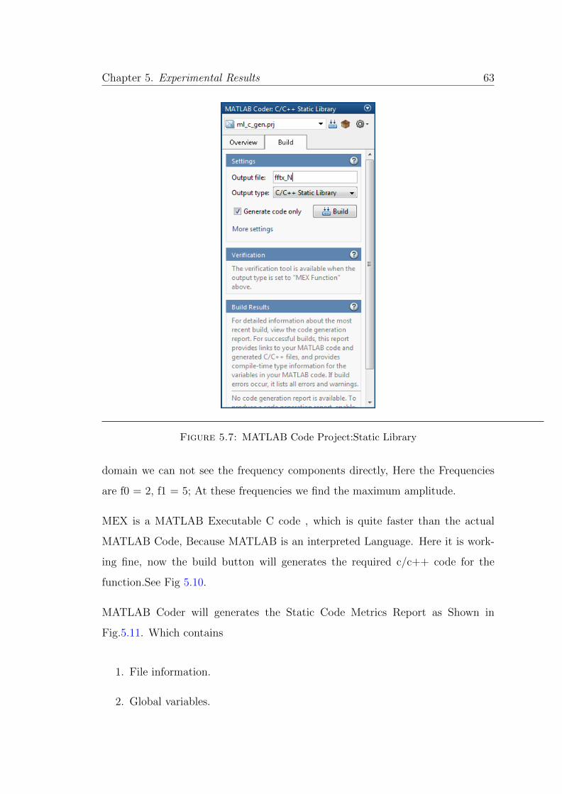
Chapter 5. Experimental Results 63
Figure 5.7: MATLAB Code Project:Static Library
domain we can not see the frequency components directly, Here the Frequencies
are f0 = 2, f1 = 5; At these frequencies we find the maximum amplitude.
MEX is a MATLAB Executable C code , which is quite faster than the actual
MATLAB Code, Because MATLAB is an interpreted Language. Here it is work-
ing fine, now the build button will generates the required c/c++ code for the
function.See Fig 5.10.
MATLAB Coder will generates the Static Code Metrics Report as Shown in
Fig.5.11. Which contains
1. File information.
2. Global variables.
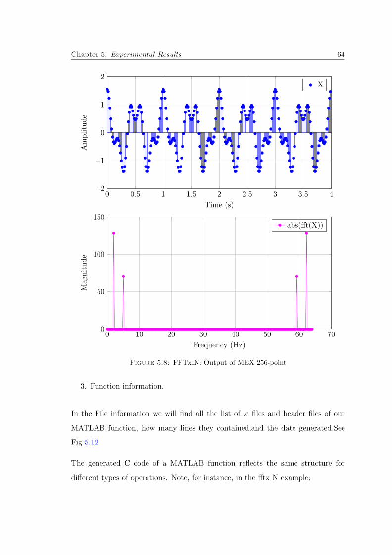
Chapter 5. Experimental Results 64
0 0.5 1 1.5 2 2.5 3 3.5 4−2
−1
0
1
2
Time (s)
Am
plitu
de
X
0 10 20 30 40 50 60 700
50
100
150
Frequency (Hz)
Mag
nit
ude
abs(fft(X))
Figure 5.8: FFTx N: Output of MEX 256-point
3. Function information.
In the File information we will find all the list of .c files and header files of our
MATLAB function, how many lines they contained,and the date generated.See
Fig 5.12
The generated C code of a MATLAB function reflects the same structure for
different types of operations. Note, for instance, in the fftx N example:
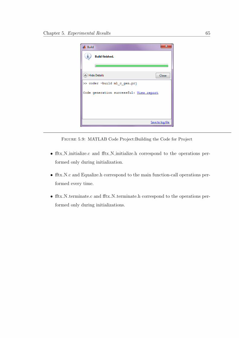
Chapter 5. Experimental Results 65
Figure 5.9: MATLAB Code Project:Building the Code for Project
• fftx N initialize.c and fftx N initialize.h correspond to the operations per-
formed only during initialization.
• fftx N.c and Equalize.h correspond to the main function-call operations per-
formed every time.
• fftx N terminate.c and fftx N terminate.h correspond to the operations per-
formed only during initializations.

Chapter 5. Experimental Results 66
Figure 5.10: MATLAB Code Project:Some lines of the Generated C Code
Figure 5.11: MATLAB Code Project:Static Code Metrics Report
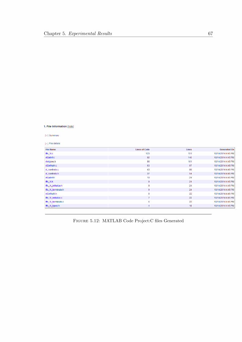
Chapter 5. Experimental Results 67
Figure 5.12: MATLAB Code Project:C files Generated
Chapter 6
Discussion of Results
6.1 Profiling
In software engineering, profiling (”program profiling”, ”software profiling”) is a
form of dynamic program analysis that measures, for example, the space (mem-
ory) or time complexity of a program, the usage of particular instructions, or the
frequency and duration of function calls. Most commonly, profiling information
serves to aid program optimization.
Profiling is achieved by instrumenting either the program source code or its binary
executable form using a tool called a profiler (or code profiler). Profilers may use
a number of different techniques, such as event-based, statistical, instrumented,
and simulation methods.
The profile function helps you debug and optimize MATLAB R© code files by track-
ing their execution time. For each MATLAB function, MATLAB local function,
or MEX-function in the file, profile records information about execution time,
number of calls, parent functions, child functions, code line hit count, and code
line execution time. Some people use profile simply to see the child functions; see
68

Chapter 6. Discussion of Results 69
also depfun for that purpose. To open the Profiler graphical user interface, use
the profile viewer syntax. By default, Profiler time is CPU time. The total time
reported by the Profiler is not the same as the time reported using the tic and toc
functions or the time you would observe using a stopwatch.
6.2 Profile Summary
The Profile Summary report presents statistics about the overall execution of the
function and provides summary statistics for each function called. The report
formats these values in four columns.
• Function Name — A list of all the functions called by the profiled function.
When first displayed, the functions are listed in order by the amount of
time they took to process. To sort the functions alphabetically, click the
Function Name link at the top of the column.
• Calls — The number of times the function was called while profiling was on.
To sort the report by the number of times functions were called, click the
Calls link at the top of the column.
• Total Time — The total time spent in a function, including all child functions
called, in seconds. The time for a function includes time spent on child
functions. To sort the functions by the amount of time they consumed, click
the Total Time link at the top of the column. By default, the summary
report displays profiling information sorted by Total Time. Be aware that
the Profiler itself uses some time, which is included in the results. Also note
that total time can be zero for files whose running time was inconsequential.
• Self Time — The total time spent in a function, not including time for any
child functions called, in seconds. If MATLAB can determine the amount of
time spent for profiling overhead, MATLAB excludes it from the self time
Chapter 6. Discussion of Results 70
also. (MATLAB excludes profiling overhead from the total time and the
time for individual lines in the Profile Detail Report as well.) The bottom
of the Profiler page contains a message like one of the following, depending
on whether MATLAB can determine the profiling overhead:
-Self time is the time spent in a function excluding:
– The time spent in its child functions
– Most of the overhead resulting from the process of profiling
• Total Time Plot — Graphic display showing self time compared to total
time.
File Listing
• The first column lists the execution time for each line.
• The second column lists the number of times the line was called
• The third column specifies the source code for the function.
In the function listing, the color of the text indicates the following:
Green — Comment lines
Black — Lines of code that executed
Gray — Lines of code that did not execute
By default, the Profile Detail report highlights lines of code with the longest
execution time. The darker the highlighting, the longer the line of code took to
execute.see Fig. 6.2
In this test-bench we have compared to functions. One is .m function and the
other is mex function , both takes same input and produce the same output with
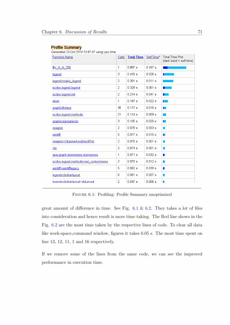
Chapter 6. Discussion of Results 71
Figure 6.1: Profiling: Profile Summary unoptimized
great amount of difference in time. See Fig. 6.1 & 6.2. They takes a lot of files
into consideration and hence result is more time taking. The Red line shows in the
Fig. 6.2 are the most time taken by the respective lines of code. To clear all data
like work-space,command window, figures it takes 0.05 s. The most time spent on
line 13, 12, 11, 1 and 16 respectively.
If we remove some of the lines from the same code, we can see the improved
performance in execution time.
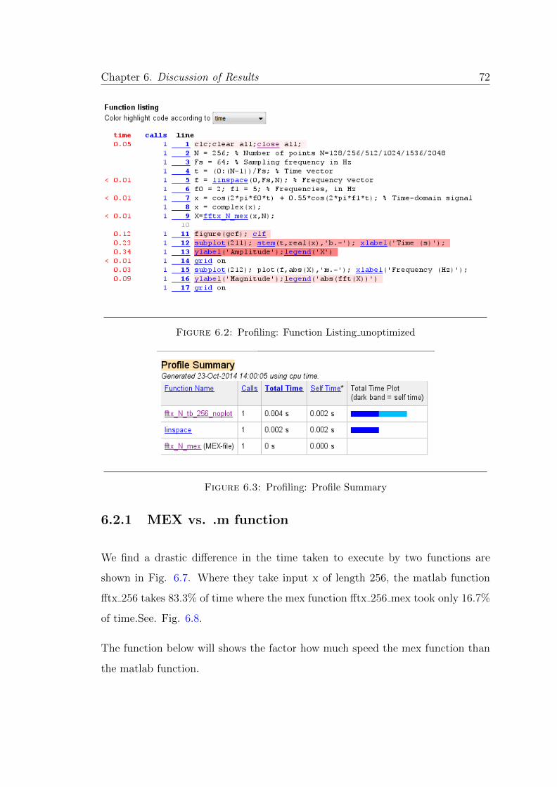
Chapter 6. Discussion of Results 72
Figure 6.2: Profiling: Function Listing unoptimized
Figure 6.3: Profiling: Profile Summary
6.2.1 MEX vs. .m function
We find a drastic difference in the time taken to execute by two functions are
shown in Fig. 6.7. Where they take input x of length 256, the matlab function
fftx 256 takes 83.3% of time where the mex function fftx 256 mex took only 16.7%
of time.See. Fig. 6.8.
The function below will shows the factor how much speed the mex function than
the matlab function.
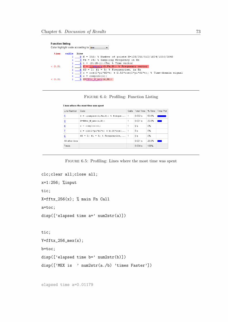
Chapter 6. Discussion of Results 73
Figure 6.4: Profiling: Function Listing
Figure 6.5: Profiling: Lines where the most time was spent
clc;clear all;close all;
x=1:256; %input
tic;
X=fftx_256(x); % main Fn Call
a=toc;
disp([’elapsed time a=’ num2str(a)])
tic;
Y=fftx_256_mex(x);
b=toc;
disp([’elapsed time b=’ num2str(b)])
disp([’MEX is ’ num2str(a./b) ’times Faster’])
elapsed time a=0.01179
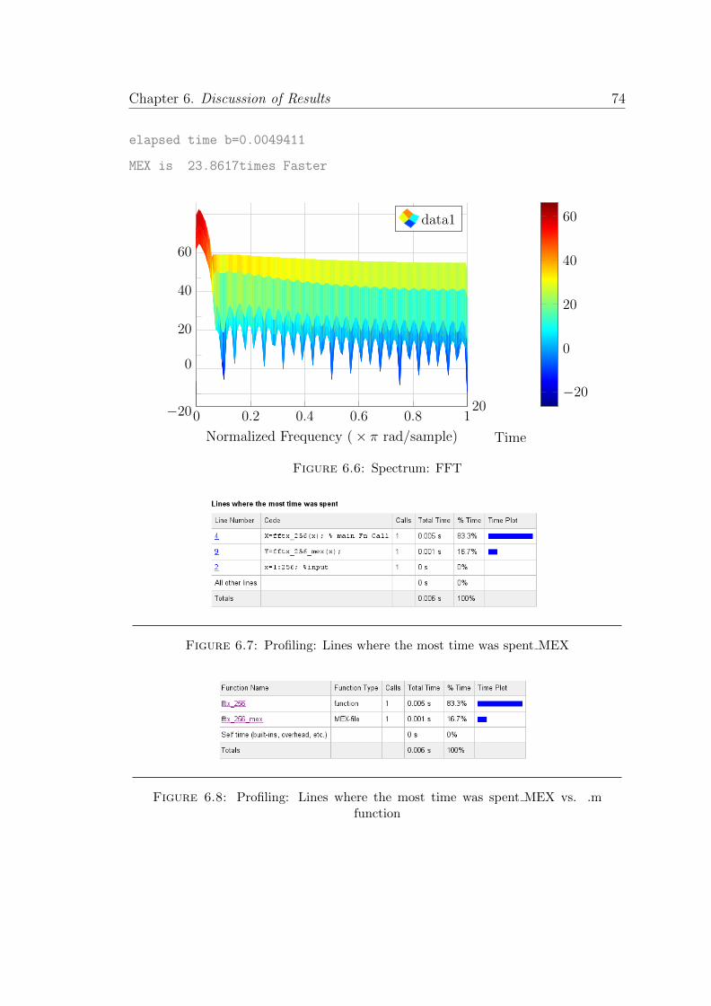
Chapter 6. Discussion of Results 74
elapsed time b=0.0049411
MEX is 23.8617times Faster
0 0.2 0.4 0.6 0.8 120−20
0
20
40
60
Normalized Frequency (× π rad/sample) Time
data1
−20
0
20
40
60
Figure 6.6: Spectrum: FFT
Figure 6.7: Profiling: Lines where the most time was spent MEX
Figure 6.8: Profiling: Lines where the most time was spent MEX vs. .mfunction

Chapter 7
Summery,Conclusion and
Reccomendations
7.1 summary
In this chapter we summarize the topics discussed in the thesis and provide a
framework for future work.In this dessertion we have discussed DFT, and it’s Faster
version i.e., FFT. We also studied Divide-and-conquer technique and implemented
an algorithm using the concept.
We have implemented algorithm in MATLAB and tested. Then we have im-
plemented C/C++ prototype to it, in order to develop the software using the
algorithm.
Modeling is very useful tool of simulink to design systems.We have analyzed mathe-
matical basis of twiddle factors, found that similarity in computation and designed
a reduced computational algorithm. Modeled it using hdllib and generated HDL
code and resource utilization report to it.
75
Chapter 7. Summery,Conclusion and Reccomendations 76
7.2 Conclusion
Mathematical algorithms are very important in every field of engineering. MAT-
LAB provides very efficient tools to prototype as well as hardware generation for
the algorithms. It saves a lot of time of designer and also cost.
7.3 Future Work
Since many years we have been using traditional way of approach to design hard-
ware i.e., by using Hardware description languages like VHDL, Verilog etc., Now
It’s time to move on for the High Level Synthesis. High level languages such
as C/C++ can be used to design Hardware. Simply Provide a C code ,and a
test-bench in vivado HLS will generates Hardware.
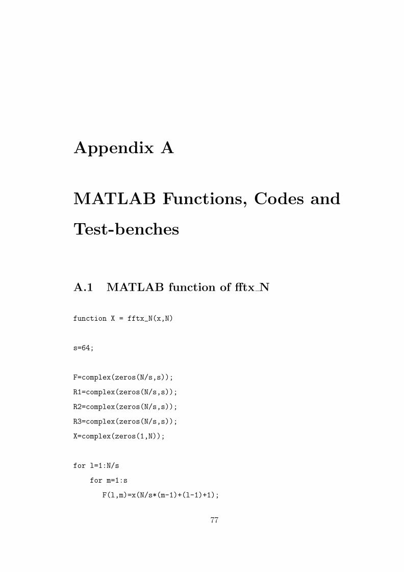
Appendix A
MATLAB Functions, Codes and
Test-benches
A.1 MATLAB function of fftx N
function X = fftx_N(x,N)
s=64;
F=complex(zeros(N/s,s));
R1=complex(zeros(N/s,s));
R2=complex(zeros(N/s,s));
R3=complex(zeros(N/s,s));
X=complex(zeros(1,N));
for l=1:N/s
for m=1:s
F(l,m)=x(N/s*(m-1)+(l-1)+1);
77

Appendix A. MATLAB Functions and Test-benches 78
end
end
m=s;
l=N/s;
wm=twdl4(m,m,m);
wl=twdl4(l,l,l);
wN=twdl4(l,m,m*l);
R1=F*wm;
R2=wN.*R1;
R3=wl*R2;
for p=1:N/s
for q=1:s
X(s*(p-1)+(q-1)+1)=R3(N/s*(q-1)+(p-1)+1);
end
end
end
function w = twdl4(p,q,N)
w=complex(zeros(p,q));
for n=1:p
for k=1:q
w(n,k)=exp((-1i*2*pi*(n-1)*(k-1))/N);
end
end
end
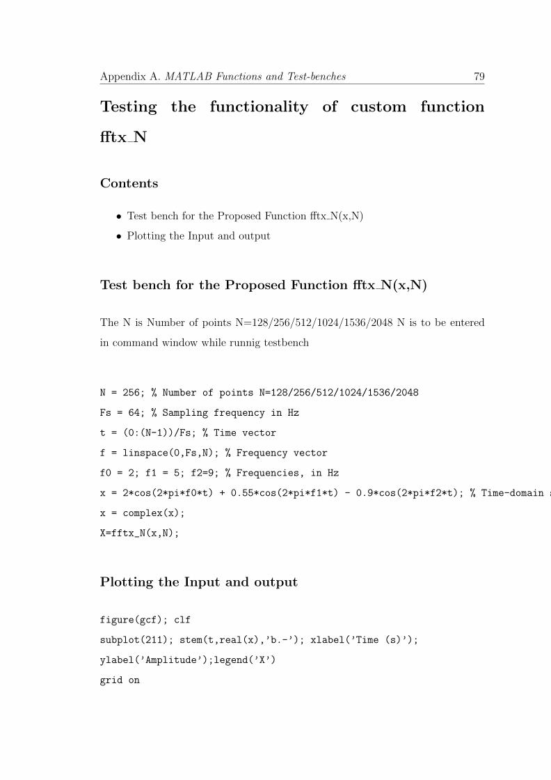
Appendix A. MATLAB Functions and Test-benches 79
Testing the functionality of custom function
fftx N
Contents
• Test bench for the Proposed Function fftx N(x,N)
• Plotting the Input and output
Test bench for the Proposed Function fftx N(x,N)
The N is Number of points N=128/256/512/1024/1536/2048 N is to be entered
in command window while runnig testbench
N = 256; % Number of points N=128/256/512/1024/1536/2048
Fs = 64; % Sampling frequency in Hz
t = (0:(N-1))/Fs; % Time vector
f = linspace(0,Fs,N); % Frequency vector
f0 = 2; f1 = 5; f2=9; % Frequencies, in Hz
x = 2*cos(2*pi*f0*t) + 0.55*cos(2*pi*f1*t) - 0.9*cos(2*pi*f2*t); % Time-domain signal
x = complex(x);
X=fftx_N(x,N);
Plotting the Input and output
figure(gcf); clf
subplot(211); stem(t,real(x),’b.-’); xlabel(’Time (s)’);
ylabel(’Amplitude’);legend(’X’)
grid on

Appendix A. MATLAB Functions and Test-benches 80
subplot(212); plot(f,abs(X),’m.-’); xlabel(’Frequency (Hz)’);
ylabel(’Magnitude’);legend(’abs(fft(X))’)
grid on
Verification of user defined function with default
fft function
clc;clear all;close all;
Fs = 1000; % Sampling frequency
T = 1/Fs; % Sample time
L = 1024; % Length of signal
t = (0:L-1)*T; % Time vector

Appendix A. MATLAB Functions and Test-benches 81
% Sum of a 50 Hz sinusoid and a 120 Hz sinusoid
x = 0.7*sin(2*pi*50*t) + sin(2*pi*120*t);
y = x + 2*randn(size(t)); % Sinusoids plus noise
figure,plot(Fs*t(1:500),y(1:500))
title(’Signal Corrupted with Zero-Mean Random Noise’)
xlabel(’time (milliseconds)’)
NFFT = 2^nextpow2(L); % Next power of 2 from length of y
display(’1.default ’)
display(’2.userdefined’)
input_fn = input(’Enter a number:’);
switch input_fn
case 1
Y = fft(y,NFFT)/L;
disp(’****default fft function output****’)
otherwise
Y = fftx_N(y,NFFT)/L;
disp(’####User defined fft function output####’)
end
f = Fs/2*linspace(0,1,NFFT/2+1);
% Plot single-sided amplitude spectrum.
figure,plot(f,2*abs(Y(1:NFFT/2+1)))
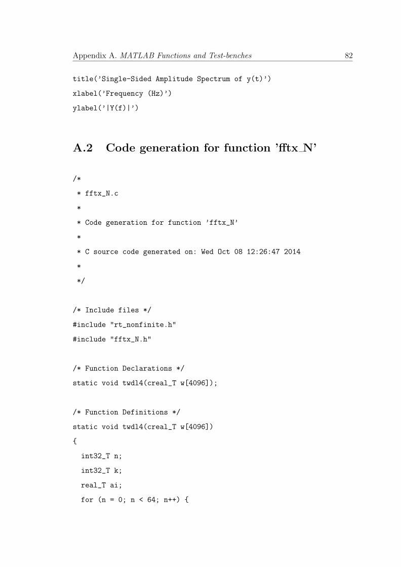
Appendix A. MATLAB Functions and Test-benches 82
title(’Single-Sided Amplitude Spectrum of y(t)’)
xlabel(’Frequency (Hz)’)
ylabel(’|Y(f)|’)
A.2 Code generation for function ’fftx N’
/*
* fftx_N.c
*
* Code generation for function ’fftx_N’
*
* C source code generated on: Wed Oct 08 12:26:47 2014
*
*/
/* Include files */
#include "rt_nonfinite.h"
#include "fftx_N.h"
/* Function Declarations */
static void twdl4(creal_T w[4096]);
/* Function Definitions */
static void twdl4(creal_T w[4096])
int32_T n;
int32_T k;
real_T ai;
for (n = 0; n < 64; n++)
Appendix A. MATLAB Functions and Test-benches 83
for (k = 0; k < 64; k++)
ai = ((1.0 + (real_T)n) - 1.0) * -6.2831853071795862 * ((1.0 + (real_T)k)
- 1.0);
if (ai == 0.0)
ai = 0.0;
else
ai /= 64.0;
w[n + (k << 6)].re = cos(ai);
w[n + (k << 6)].im = sin(ai);
void fftx_N(const int8_T x[256], creal_T X[256])
int32_T l;
cint8_T F[256];
int32_T q;
creal_T wm[4096];
creal_T b_F[256];
int32_T i0;
creal_T wN[256];
static const creal_T b_wN[256] = 1.0, 0.0 , 1.0, 0.0 , 1.0, 0.0 ,
1.0, 0.0 , 1.0, 0.0 , 0.99969881869620425, -0.024541228522912288 ,
0.99879545620517241, -0.049067674327418015 , 0.99729045667869021,
-0.073564563599667426 , 1.0, 0.0 , 0.99879545620517241,
-0.049067674327418015 , 0.99518472667219693, -0.0980171403295606 ,
Appendix A. MATLAB Functions and Test-benches 84
0.989176509964781, -0.14673047445536175 , 1.0, 0.0 ,
0.99729045667869021, -0.073564563599667426 , 0.989176509964781,
-0.14673047445536175 , 0.97570213003852857, -0.2191012401568698 ,
1.0, 0.0 , 0.99518472667219693, -0.0980171403295606 ,
0.98078528040323043, -0.19509032201612825 , 0.95694033573220882,
-0.29028467725446233 , 1.0, 0.0 , 0.99247953459871,
-0.1224106751992162 , 0.970031253194544, -0.24298017990326387 ,
0.932992798834739, -0.35989503653498811 , 1.0, 0.0 ,
0.989176509964781, -0.14673047445536175 , 0.95694033573220882,
-0.29028467725446233 , 0.90398929312344334, -0.42755509343028208 ,
1.0, 0.0 , 0.98527764238894122, -0.17096188876030122 ,
0.94154406518302081, -0.33688985339222005 , 0.87008699110871146,
-0.49289819222978404 , 1.0, 0.0 , 0.98078528040323043,
-0.19509032201612825 , 0.92387953251128674, -0.38268343236508978 ,
0.83146961230254524, -0.55557023301960218 , 1.0, 0.0 ,
0.97570213003852857, -0.2191012401568698 , 0.90398929312344334,
-0.42755509343028208 , 0.78834642762660634, -0.61523159058062682 ,
1.0, 0.0 , 0.970031253194544, -0.24298017990326387 ,
0.881921264348355, -0.47139673682599764 , 0.74095112535495922,
-0.67155895484701833 , 1.0, 0.0 , 0.96377606579543984,
-0.26671275747489837 , 0.85772861000027212, -0.51410274419322166 ,
0.68954054473706694, -0.72424708295146689 , 1.0, 0.0 ,
0.95694033573220882, -0.29028467725446233 , 0.83146961230254524,
-0.55557023301960218 , 0.63439328416364549, -0.77301045336273688 ,
1.0, 0.0 , 0.94952818059303667, -0.31368174039889152 ,
0.80320753148064494, -0.59569930449243336 , 0.57580819141784534,
-0.81758481315158371 , 1.0, 0.0 , 0.94154406518302081,
-0.33688985339222005 , 0.773010453362737, -0.63439328416364549 ,
0.51410274419322166, -0.85772861000027212 , 1.0, 0.0 ,
Appendix A. MATLAB Functions and Test-benches 85
0.932992798834739, -0.35989503653498811 , 0.74095112535495922,
-0.67155895484701833 , 0.4496113296546066, -0.89322430119551532 ,
1.0, 0.0 , 0.92387953251128674, -0.38268343236508978 ,
0.70710678118654757, -0.70710678118654746 , 0.38268343236508984,
-0.92387953251128674 , 1.0, 0.0 , 0.91420975570353069,
-0.40524131400498986 , 0.67155895484701844, -0.74095112535495911 ,
0.31368174039889157, -0.94952818059303667 , 1.0, 0.0 ,
0.90398929312344334, -0.42755509343028208 , 0.63439328416364549,
-0.77301045336273688 , 0.24298017990326398, -0.970031253194544 , 1.0,
0.0 , 0.89322430119551532, -0.44961132965460654 ,
0.59569930449243347, -0.80320753148064483 , 0.17096188876030136,
-0.98527764238894122 , 1.0, 0.0 , 0.881921264348355,
-0.47139673682599764 , 0.55557023301960229, -0.83146961230254524 ,
0.09801714032956077, -0.99518472667219682 , 1.0, 0.0 ,
0.87008699110871146, -0.49289819222978404 , 0.51410274419322166,
-0.85772861000027212 , 0.024541228522912264, -0.99969881869620425 ,
1.0, 0.0 , 0.85772861000027212, -0.51410274419322166 ,
0.47139673682599781, -0.88192126434835494 , -0.049067674327418008,
-0.99879545620517241 , 1.0, 0.0 , 0.84485356524970712,
-0.53499761988709715 , 0.4275550934302822, -0.90398929312344334 , -
0.12241067519921615, -0.99247953459871 , 1.0, 0.0 ,
0.83146961230254524, -0.55557023301960218 , 0.38268343236508984,
-0.92387953251128674 , -0.19509032201612819, -0.98078528040323043 ,
1.0, 0.0 , 0.81758481315158371, -0.57580819141784534 ,
0.33688985339222005, -0.94154406518302081 , -0.26671275747489831,
-0.96377606579543984 , 1.0, 0.0 , 0.80320753148064494,
-0.59569930449243336 , 0.29028467725446233, -0.95694033573220894 , -
0.33688985339221994, -0.94154406518302081 , 1.0, 0.0 ,
0.78834642762660634, -0.61523159058062682 , 0.24298017990326398,

Appendix A. MATLAB Functions and Test-benches 86
-0.970031253194544 , -0.40524131400498975, -0.91420975570353069 ,
1.0, 0.0 , 0.773010453362737, -0.63439328416364549 ,
0.19509032201612833, -0.98078528040323043 , -0.4713967368259977,
-0.881921264348355 , 1.0, 0.0 , 0.75720884650648457,
-0.65317284295377676 , 0.14673047445536175, -0.989176509964781 , -
0.534997619887097, -0.84485356524970723 , 1.0, 0.0 ,
0.74095112535495922, -0.67155895484701833 , 0.09801714032956077,
-0.99518472667219682 , -0.59569930449243336, -0.80320753148064494 ,
1.0, 0.0 , 0.724247082951467, -0.68954054473706683 ,
0.049067674327418126, -0.99879545620517241 , -0.65317284295377653,
-0.75720884650648468 , 1.0, 0.0 , 0.70710678118654757,
-0.70710678118654746 , 6.123233995736766E-17, -1.0 , -
0.70710678118654746, -0.70710678118654757 , 1.0, 0.0 ,
0.68954054473706694, -0.72424708295146689 , -0.049067674327418008,
-0.99879545620517241 , -0.75720884650648468, -0.65317284295377664 ,
1.0, 0.0 , 0.67155895484701844, -0.74095112535495911 , -
0.098017140329560645, -0.99518472667219693 , -0.80320753148064483,
-0.59569930449243347 , 1.0, 0.0 , 0.65317284295377687,
-0.75720884650648457 , -0.14673047445536164, -0.989176509964781 , -
0.84485356524970712, -0.53499761988709715 , 1.0, 0.0 ,
0.63439328416364549, -0.77301045336273688 , -0.19509032201612819,
-0.98078528040323043 , -0.88192126434835494, -0.47139673682599786 ,
1.0, 0.0 , 0.61523159058062682, -0.78834642762660623 , -
0.24298017990326387, -0.970031253194544 , -0.91420975570353069,
-0.40524131400498992 , 1.0, 0.0 , 0.59569930449243347,
-0.80320753148064483 , -0.29028467725446216, -0.95694033573220894 ,
-0.9415440651830207, -0.33688985339222033 , 1.0, 0.0 ,
0.57580819141784534, -0.81758481315158371 , -0.33688985339221994,
-0.94154406518302081 , -0.96377606579543984, -0.26671275747489848 ,
Appendix A. MATLAB Functions and Test-benches 87
1.0, 0.0 , 0.55557023301960229, -0.83146961230254524 , -
0.38268343236508973, -0.92387953251128674 , -0.98078528040323043,
-0.19509032201612861 , 1.0, 0.0 , 0.53499761988709726,
-0.844853565249707 , -0.42755509343028186, -0.90398929312344345 , -
0.99247953459871, -0.12241067519921635 , 1.0, 0.0 ,
0.51410274419322166, -0.85772861000027212 , -0.4713967368259977,
-0.881921264348355 , -0.99879545620517241, -0.049067674327417966 ,
1.0, 0.0 , 0.49289819222978409, -0.87008699110871135 , -
0.51410274419322155, -0.85772861000027212 , -0.99969881869620425,
0.02454122852291208 , 1.0, 0.0 , 0.47139673682599781,
-0.88192126434835494 , -0.555570233019602, -0.83146961230254535 , -
0.99518472667219693, 0.09801714032956059 , 1.0, 0.0 ,
0.4496113296546066, -0.89322430119551532 , -0.59569930449243336,
-0.80320753148064494 , -0.98527764238894133, 0.17096188876030097 ,
1.0, 0.0 , 0.4275550934302822, -0.90398929312344334 , -
0.63439328416364538, -0.7730104533627371 , -0.970031253194544,
0.24298017990326382 , 1.0, 0.0 , 0.40524131400498986,
-0.91420975570353069 , -0.67155895484701844, -0.740951125354959 , -
0.94952818059303679, 0.31368174039889118 , 1.0, 0.0 ,
0.38268343236508984, -0.92387953251128674 , -0.70710678118654746,
-0.70710678118654757 , -0.92387953251128685, 0.38268343236508967 ,
1.0, 0.0 , 0.35989503653498828, -0.93299279883473885 , -
0.74095112535495888, -0.67155895484701855 , -0.89322430119551532,
0.44961132965460665 , 1.0, 0.0 , 0.33688985339222005,
-0.94154406518302081 , -0.773010453362737, -0.63439328416364549 , -
0.85772861000027212, 0.51410274419322155 , 1.0, 0.0 ,
0.31368174039889157, -0.94952818059303667 , -0.80320753148064483,
-0.59569930449243347 , -0.81758481315158371, 0.57580819141784534 ,
1.0, 0.0 , 0.29028467725446233, -0.95694033573220894 , -
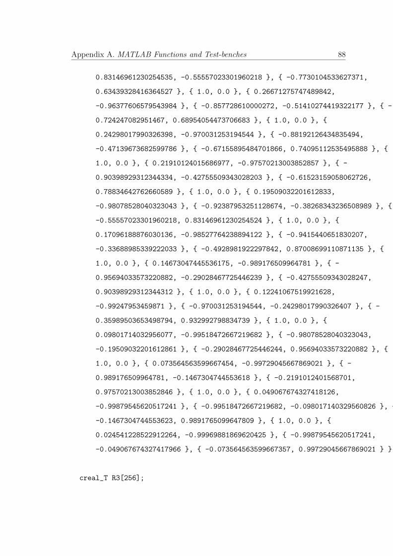
Appendix A. MATLAB Functions and Test-benches 88
0.83146961230254535, -0.55557023301960218 , -0.7730104533627371,
0.63439328416364527 , 1.0, 0.0 , 0.26671275747489842,
-0.96377606579543984 , -0.857728610000272, -0.51410274419322177 , -
0.724247082951467, 0.68954054473706683 , 1.0, 0.0 ,
0.24298017990326398, -0.970031253194544 , -0.88192126434835494,
-0.47139673682599786 , -0.67155895484701866, 0.74095112535495888 ,
1.0, 0.0 , 0.21910124015686977, -0.97570213003852857 , -
0.90398929312344334, -0.42755509343028203 , -0.61523159058062726,
0.78834642762660589 , 1.0, 0.0 , 0.19509032201612833,
-0.98078528040323043 , -0.92387953251128674, -0.38268343236508989 ,
-0.55557023301960218, 0.83146961230254524 , 1.0, 0.0 ,
0.17096188876030136, -0.98527764238894122 , -0.9415440651830207,
-0.33688985339222033 , -0.4928981922297842, 0.87008699110871135 ,
1.0, 0.0 , 0.14673047445536175, -0.989176509964781 , -
0.95694033573220882, -0.29028467725446239 , -0.42755509343028247,
0.90398929312344312 , 1.0, 0.0 , 0.12241067519921628,
-0.99247953459871 , -0.970031253194544, -0.24298017990326407 , -
0.35989503653498794, 0.932992798834739 , 1.0, 0.0 ,
0.09801714032956077, -0.99518472667219682 , -0.98078528040323043,
-0.19509032201612861 , -0.29028467725446244, 0.95694033573220882 ,
1.0, 0.0 , 0.073564563599667454, -0.99729045667869021 , -
0.989176509964781, -0.1467304744553618 , -0.2191012401568701,
0.97570213003852846 , 1.0, 0.0 , 0.049067674327418126,
-0.99879545620517241 , -0.99518472667219682, -0.098017140329560826 ,
-0.1467304744553623, 0.9891765099647809 , 1.0, 0.0 ,
0.024541228522912264, -0.99969881869620425 , -0.99879545620517241,
-0.049067674327417966 , -0.073564563599667357, 0.99729045667869021 ;
creal_T R3[256];
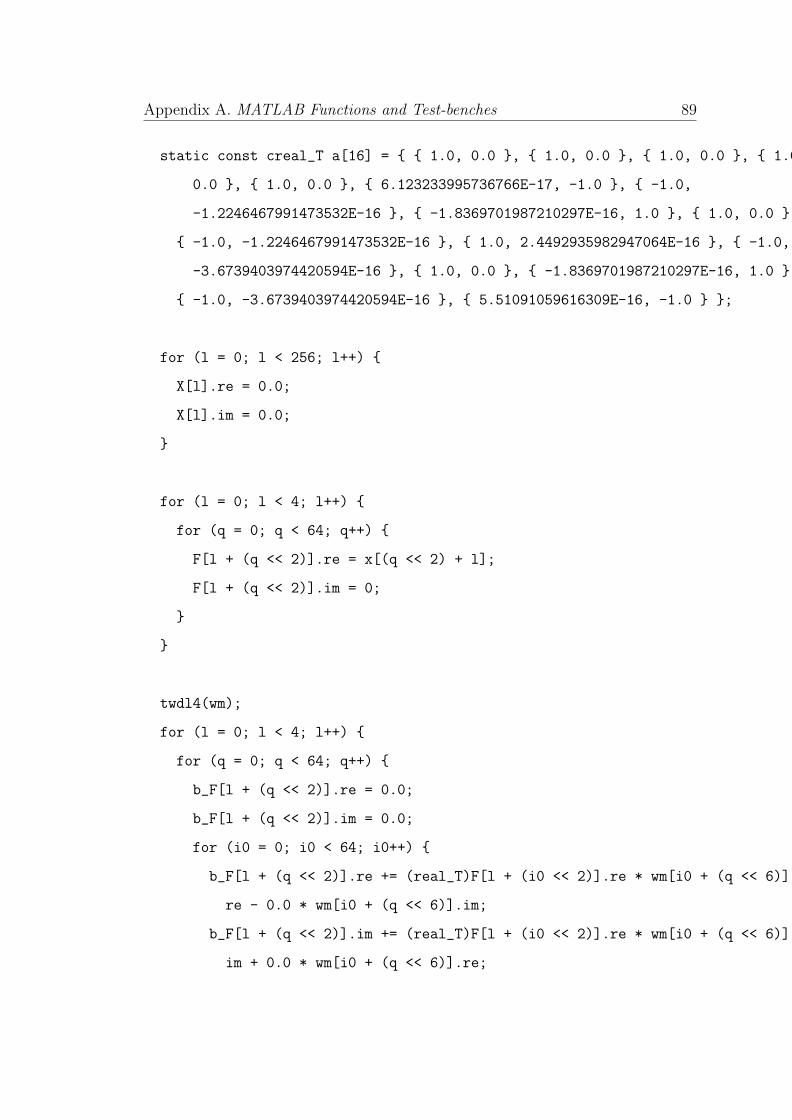
Appendix A. MATLAB Functions and Test-benches 89
static const creal_T a[16] = 1.0, 0.0 , 1.0, 0.0 , 1.0, 0.0 , 1.0,
0.0 , 1.0, 0.0 , 6.123233995736766E-17, -1.0 , -1.0,
-1.2246467991473532E-16 , -1.8369701987210297E-16, 1.0 , 1.0, 0.0 ,
-1.0, -1.2246467991473532E-16 , 1.0, 2.4492935982947064E-16 , -1.0,
-3.6739403974420594E-16 , 1.0, 0.0 , -1.8369701987210297E-16, 1.0 ,
-1.0, -3.6739403974420594E-16 , 5.51091059616309E-16, -1.0 ;
for (l = 0; l < 256; l++)
X[l].re = 0.0;
X[l].im = 0.0;
for (l = 0; l < 4; l++)
for (q = 0; q < 64; q++)
F[l + (q << 2)].re = x[(q << 2) + l];
F[l + (q << 2)].im = 0;
twdl4(wm);
for (l = 0; l < 4; l++)
for (q = 0; q < 64; q++)
b_F[l + (q << 2)].re = 0.0;
b_F[l + (q << 2)].im = 0.0;
for (i0 = 0; i0 < 64; i0++)
b_F[l + (q << 2)].re += (real_T)F[l + (i0 << 2)].re * wm[i0 + (q << 6)].
re - 0.0 * wm[i0 + (q << 6)].im;
b_F[l + (q << 2)].im += (real_T)F[l + (i0 << 2)].re * wm[i0 + (q << 6)].
im + 0.0 * wm[i0 + (q << 6)].re;
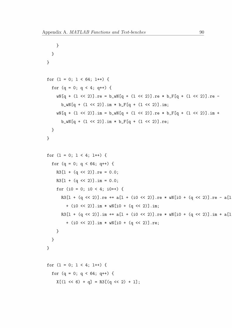
Appendix A. MATLAB Functions and Test-benches 90
for (l = 0; l < 64; l++)
for (q = 0; q < 4; q++)
wN[q + (l << 2)].re = b_wN[q + (l << 2)].re * b_F[q + (l << 2)].re -
b_wN[q + (l << 2)].im * b_F[q + (l << 2)].im;
wN[q + (l << 2)].im = b_wN[q + (l << 2)].re * b_F[q + (l << 2)].im +
b_wN[q + (l << 2)].im * b_F[q + (l << 2)].re;
for (l = 0; l < 4; l++)
for (q = 0; q < 64; q++)
R3[l + (q << 2)].re = 0.0;
R3[l + (q << 2)].im = 0.0;
for (i0 = 0; i0 < 4; i0++)
R3[l + (q << 2)].re += a[l + (i0 << 2)].re * wN[i0 + (q << 2)].re - a[l
+ (i0 << 2)].im * wN[i0 + (q << 2)].im;
R3[l + (q << 2)].im += a[l + (i0 << 2)].re * wN[i0 + (q << 2)].im + a[l
+ (i0 << 2)].im * wN[i0 + (q << 2)].re;
for (l = 0; l < 4; l++)
for (q = 0; q < 64; q++)
X[(l << 6) + q] = R3[(q << 2) + l];

Appendix A. MATLAB Functions and Test-benches 91
/* End of code generation (fftx_N.c) */
A.3 Processing Element.vhd
-- -------------------------------------------------------------
--
-- File Name: hdl_prj\hdlsrc\r4sqr_hdl_16pt_3rd_stg_setup\Processing_Element.vhd
-- Created: 2014-10-15 22:04:28
--
-- Generated by MATLAB 8.1 and HDL Coder 3.2
--
--
-- -------------------------------------------------------------
-- Rate and Clocking Details
-- -------------------------------------------------------------
-- Model base rate: 0.2
-- Target subsystem base rate: 0.2
--
-- -------------------------------------------------------------
-- -------------------------------------------------------------
--
-- Module: Processing_Element
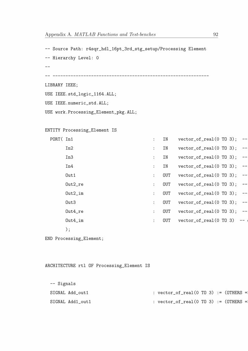
Appendix A. MATLAB Functions and Test-benches 92
-- Source Path: r4sqr_hdl_16pt_3rd_stg_setup/Processing Element
-- Hierarchy Level: 0
--
-- -------------------------------------------------------------
LIBRARY IEEE;
USE IEEE.std_logic_1164.ALL;
USE IEEE.numeric_std.ALL;
USE work.Processing_Element_pkg.ALL;
ENTITY Processing_Element IS
PORT( In1 : IN vector_of_real(0 TO 3); -- double [4]
In2 : IN vector_of_real(0 TO 3); -- double [4]
In3 : IN vector_of_real(0 TO 3); -- double [4]
In4 : IN vector_of_real(0 TO 3); -- double [4]
Out1 : OUT vector_of_real(0 TO 3); -- double [4]
Out2_re : OUT vector_of_real(0 TO 3); -- double [4]
Out2_im : OUT vector_of_real(0 TO 3); -- double [4]
Out3 : OUT vector_of_real(0 TO 3); -- double [4]
Out4_re : OUT vector_of_real(0 TO 3); -- double [4]
Out4_im : OUT vector_of_real(0 TO 3) -- double [4]
);
END Processing_Element;
ARCHITECTURE rtl OF Processing_Element IS
-- Signals
SIGNAL Add_out1 : vector_of_real(0 TO 3) := (OTHERS => 0.0); -- double [4]
SIGNAL Add1_out1 : vector_of_real(0 TO 3) := (OTHERS => 0.0); -- double [4]
Appendix A. MATLAB Functions and Test-benches 93
SIGNAL Add2_out1 : vector_of_real(0 TO 3) := (OTHERS => 0.0); -- double [4]
SIGNAL Subtract_out1 : vector_of_real(0 TO 3) := (OTHERS => 0.0); -- double [4]
SIGNAL Subtract1_out1 : vector_of_real(0 TO 3) := (OTHERS => 0.0); -- double [4]
SIGNAL Constant4_out1_re : real := 0.0; -- double
SIGNAL Constant4_out1_im : real := 0.0; -- double
SIGNAL Product_out1_re : vector_of_real(0 TO 3) := (OTHERS => 0.0); -- double [4]
SIGNAL Product_out1_im : vector_of_real(0 TO 3) := (OTHERS => 0.0); -- double [4]
SIGNAL Add3_out1_re : vector_of_real(0 TO 3) := (OTHERS => 0.0); -- double [4]
SIGNAL Add3_out1_im : vector_of_real(0 TO 3) := (OTHERS => 0.0); -- double [4]
SIGNAL Subtract2_out1 : vector_of_real(0 TO 3) := (OTHERS => 0.0); -- double [4]
SIGNAL Subtract3_out1_re : vector_of_real(0 TO 3) := (OTHERS => 0.0); -- double [4]
SIGNAL Subtract3_out1_im : vector_of_real(0 TO 3) := (OTHERS => 0.0); -- double [4]
BEGIN
-- <S1>/Add
Add_out1_gen: FOR t_0 IN 0 TO 3 GENERATE
Add_out1(t_0) <= In1(t_0) + In2(t_0);
END GENERATE Add_out1_gen;
-- <S1>/Add1
Add1_out1_gen: FOR t_01 IN 0 TO 3 GENERATE
Add1_out1(t_01) <= In3(t_01) + In4(t_01);
END GENERATE Add1_out1_gen;
-- <S1>/Add2

Appendix A. MATLAB Functions and Test-benches 94
Add2_out1_gen: FOR t_02 IN 0 TO 3 GENERATE
Add2_out1(t_02) <= Add_out1(t_02) + Add1_out1(t_02);
END GENERATE Add2_out1_gen;
-- <S1>/Subtract
Subtract_out1_gen: FOR t_03 IN 0 TO 3 GENERATE
Subtract_out1(t_03) <= In1(t_03) - In2(t_03);
END GENERATE Subtract_out1_gen;
-- <S1>/Subtract1
Subtract1_out1_gen: FOR t_04 IN 0 TO 3 GENERATE
Subtract1_out1(t_04) <= In3(t_04) - In4(t_04);
END GENERATE Subtract1_out1_gen;
-- <S1>/Constant4
Constant4_out1_re <= 0.0;
Constant4_out1_im <= 1.0;
-- <S1>/Product
Product_out1_re(0) <= Subtract1_out1(0) * Constant4_out1_re;
Product_out1_im(0) <= Subtract1_out1(0) * Constant4_out1_im;
Product_out1_re(1) <= Subtract1_out1(1) * Constant4_out1_re;
Product_out1_im(1) <= Subtract1_out1(1) * Constant4_out1_im;

Appendix A. MATLAB Functions and Test-benches 95
Product_out1_re(2) <= Subtract1_out1(2) * Constant4_out1_re;
Product_out1_im(2) <= Subtract1_out1(2) * Constant4_out1_im;
Product_out1_re(3) <= Subtract1_out1(3) * Constant4_out1_re;
Product_out1_im(3) <= Subtract1_out1(3) * Constant4_out1_im;
-- <S1>/Add3
Add3_out1_im_gen: FOR t_05 IN 0 TO 3 GENERATE
Add3_out1_re(t_05) <= Subtract_out1(t_05) + Product_out1_re(t_05);
Add3_out1_im(t_05) <= Product_out1_im(t_05);
END GENERATE Add3_out1_im_gen;
-- <S1>/Subtract2
Subtract2_out1_gen: FOR t_06 IN 0 TO 3 GENERATE
Subtract2_out1(t_06) <= Add_out1(t_06) - Add1_out1(t_06);
END GENERATE Subtract2_out1_gen;
-- <S1>/Subtract3
Subtract3_out1_im_gen: FOR t_07 IN 0 TO 3 GENERATE
Subtract3_out1_re(t_07) <= Subtract_out1(t_07) - Product_out1_re(t_07);
Subtract3_out1_im(t_07) <= - (Product_out1_im(t_07));
END GENERATE Subtract3_out1_im_gen;
Out1 <= Add2_out1;
Appendix A. MATLAB Functions and Test-benches 96
Out2_re <= Add3_out1_re;
Out2_im <= Add3_out1_im;
Out3 <= Subtract2_out1;
Out4_re <= Subtract3_out1_re;
Out4_im <= Subtract3_out1_im;
END rtl;
A.4 Processing Element tb.vhd
-- -------------------------------------------------------------
--
-- Module: Processing_Element_tb
-- Path: hdl_prj\hdlsrc\r4sqr_hdl_16pt_3rd_stg_setup
-- Created: 2014-10-15 22:04:37
-- Generated by MATLAB 8.1 and HDL Coder 3.2
-- Hierarchy Level: 1
--
--
-- -------------------------------------------------------------
LIBRARY IEEE;
USE IEEE.std_logic_1164.all;

Appendix A. MATLAB Functions and Test-benches 97
USE IEEE.numeric_std.ALL;
USE work.Processing_Element_pkg.ALL;
USE work.Processing_Element_tb_pkg.ALL;
USE work.Processing_Element_tb_data.ALL;
ENTITY Processing_Element_tb IS
END Processing_Element_tb;
ARCHITECTURE rtl OF Processing_Element_tb IS
-- -------------------------------------------------------------
-- Component Declarations
-- -------------------------------------------------------------
COMPONENT Processing_Element
PORT( In1 : IN vector_of_real(0 TO 3); -- double
In2 : IN vector_of_real(0 TO 3); -- double
In3 : IN vector_of_real(0 TO 3); -- double
In4 : IN vector_of_real(0 TO 3); -- double
Out1 : OUT vector_of_real(0 TO 3); -- double
Out2_re : OUT vector_of_real(0 TO 3); -- double
Out2_im : OUT vector_of_real(0 TO 3); -- double
Out3 : OUT vector_of_real(0 TO 3); -- double
Out4_re : OUT vector_of_real(0 TO 3); -- double
Out4_im : OUT vector_of_real(0 TO 3) -- double
);
END COMPONENT;

Appendix A. MATLAB Functions and Test-benches 98
-- -------------------------------------------------------------
-- Component Configuration Statements
-- -------------------------------------------------------------
FOR ALL : Processing_Element
USE ENTITY work.Processing_Element(rtl);
-- Constants
CONSTANT clk_high : time := 5 ns;
CONSTANT clk_low : time := 5 ns;
CONSTANT clk_period : time := 10 ns;
CONSTANT clk_hold : time := 2 ns;
CONSTANT MAX_TIMEOUT : integer := 1; -- uint32
CONSTANT MAX_ERROR_COUNT : integer := 51; -- uint32
-- Signals
SIGNAL In1 : vector_of_real(0 TO 3) := (0.0,0.0,0.0, 0.0); -- double
SIGNAL In2 : vector_of_real(0 TO 3) := (0.0,0.0,0.0, 0.0); -- double
SIGNAL In3 : vector_of_real(0 TO 3) := (0.0,0.0,0.0, 0.0); -- double
SIGNAL In4 : vector_of_real(0 TO 3) := (0.0,0.0,0.0, 0.0); -- double
SIGNAL Out1 : vector_of_real(0 TO 3) := (0.0,0.0,0.0, 0.0); -- double
SIGNAL Out2_re : vector_of_real(0 TO 3) := (0.0,0.0,0.0, 0.0); -- double
SIGNAL Out2_im : vector_of_real(0 TO 3) := (0.0,0.0,0.0, 0.0); -- double
SIGNAL Out3 : vector_of_real(0 TO 3) := (0.0,0.0,0.0, 0.0); -- double
SIGNAL Out4_re : vector_of_real(0 TO 3) := (0.0,0.0,0.0, 0.0); -- double
SIGNAL Out4_im : vector_of_real(0 TO 3) := (0.0,0.0,0.0, 0.0); -- double
SIGNAL clk : std_logic; -- boolean
SIGNAL reset : std_logic; -- boolean

Appendix A. MATLAB Functions and Test-benches 99
SIGNAL clk_enable : std_logic; -- boolean
SIGNAL tb_enb : std_logic; -- boolean
SIGNAL srcDone : std_logic; -- boolean
SIGNAL snkDone : std_logic; -- boolean
SIGNAL testFailure : std_logic; -- boolean
SIGNAL tbenb_dly : std_logic; -- boolean
SIGNAL rdEnb : std_logic; -- boolean
SIGNAL Constant_out1_rdenb : std_logic; -- boolean
SIGNAL Constant_out1_addr : unsigned(5 DOWNTO 0); -- ufix6
SIGNAL Constant_out1_done : std_logic; -- boolean
SIGNAL Constant1_out1_rdenb : std_logic; -- boolean
SIGNAL Constant1_out1_addr : unsigned(5 DOWNTO 0); -- ufix6
SIGNAL Constant1_out1_done : std_logic; -- boolean
SIGNAL Constant2_out1_rdenb : std_logic; -- boolean
SIGNAL Constant2_out1_addr : unsigned(5 DOWNTO 0); -- ufix6
SIGNAL Constant2_out1_done : std_logic; -- boolean
SIGNAL Constant3_out1_rdenb : std_logic; -- boolean
SIGNAL Constant3_out1_addr : unsigned(5 DOWNTO 0); -- ufix6
SIGNAL Constant3_out1_done : std_logic; -- boolean
SIGNAL Out1_testFailure : std_logic; -- boolean
SIGNAL Out1_timeout : integer; -- uint32
SIGNAL Out1_errCnt : integer; -- uint32
SIGNAL delayLine_out : std_logic; -- boolean
SIGNAL ce_out : std_logic; -- boolean
SIGNAL Out1_rdenb : std_logic; -- boolean
SIGNAL Out1_addr : unsigned(5 DOWNTO 0); -- ufix6
SIGNAL Out1_done : std_logic; -- boolean
SIGNAL Out1_ref : vector_of_real(0 TO 3); -- double
SIGNAL check1_Done : std_logic; -- boolean
Appendix A. MATLAB Functions and Test-benches 100
SIGNAL Out2_re_testFailure : std_logic; -- boolean
SIGNAL Out2_re_timeout : integer; -- uint32
SIGNAL Out2_re_errCnt : integer; -- uint32
SIGNAL Out2_im_errCnt : integer; -- uint32
SIGNAL Out2_re_rdenb : std_logic; -- boolean
SIGNAL Out2_re_addr : unsigned(5 DOWNTO 0); -- ufix6
SIGNAL Out2_re_done : std_logic; -- boolean
SIGNAL Out2_re_ref : vector_of_real(0 TO 3); -- double
SIGNAL Out2_im_ref : vector_of_real(0 TO 3); -- double
SIGNAL check2_Done : std_logic; -- boolean
SIGNAL Out3_testFailure : std_logic; -- boolean
SIGNAL Out3_timeout : integer; -- uint32
SIGNAL Out3_errCnt : integer; -- uint32
SIGNAL Out3_rdenb : std_logic; -- boolean
SIGNAL Out3_addr : unsigned(5 DOWNTO 0); -- ufix6
SIGNAL Out3_done : std_logic; -- boolean
SIGNAL Out3_ref : vector_of_real(0 TO 3); -- double
SIGNAL check3_Done : std_logic; -- boolean
SIGNAL Out4_re_testFailure : std_logic; -- boolean
SIGNAL Out4_re_timeout : integer; -- uint32
SIGNAL Out4_re_errCnt : integer; -- uint32
SIGNAL Out4_im_errCnt : integer; -- uint32
SIGNAL Out4_re_rdenb : std_logic; -- boolean
SIGNAL Out4_re_addr : unsigned(5 DOWNTO 0); -- ufix6
SIGNAL Out4_re_done : std_logic; -- boolean
SIGNAL Out4_re_ref : vector_of_real(0 TO 3); -- double
SIGNAL Out4_im_ref : vector_of_real(0 TO 3); -- double
SIGNAL check4_Done : std_logic; -- boolean

Appendix A. MATLAB Functions and Test-benches 101
BEGIN
-- Component Instances
u_Processing_Element: Processing_Element
PORT MAP (
In1 => In1,
In2 => In2,
In3 => In3,
In4 => In4,
Out1 => Out1,
Out2_re => Out2_re,
Out2_im => Out2_im,
Out3 => Out3,
Out4_re => Out4_re,
Out4_im => Out4_im );
-- Block Statements
-- -------------------------------------------------------------
-- Driving the test bench enable
-- -------------------------------------------------------------
tb_enb <= ’0’ WHEN reset = ’1’ ELSE
’1’ WHEN snkDone = ’0’ ELSE
’0’ AFTER clk_period * 2;
completed_msg: PROCESS (clk, reset)
BEGIN
IF (reset = ’1’) THEN

Appendix A. MATLAB Functions and Test-benches 102
-- Nothing to reset here.
ELSIF clk’event AND clk = ’1’ THEN
IF snkDone=’1’ THEN
IF (testFailure = ’0’) THEN
ASSERT FALSE
REPORT "**************TEST COMPLETED (PASSED)**************"
SEVERITY NOTE;
ELSE
ASSERT FALSE
REPORT "**************TEST COMPLETED (FAILED)**************"
SEVERITY NOTE;
END IF;
END IF;
END IF;
END PROCESS completed_msg;
-- -------------------------------------------------------------
-- System Clock (fast clock) and reset
-- -------------------------------------------------------------
clk_gen: PROCESS
BEGIN
clk <= ’1’;
WAIT FOR clk_high;
clk <= ’0’;
WAIT FOR clk_low;
IF snkDone = ’1’ THEN
clk <= ’1’;
WAIT FOR clk_high;

Appendix A. MATLAB Functions and Test-benches 103
clk <= ’0’;
WAIT FOR clk_low;
WAIT;
END IF;
END PROCESS clk_gen;
reset_gen: PROCESS
BEGIN
reset <= ’1’;
WAIT FOR clk_period * 2;
WAIT UNTIL clk’event AND clk = ’1’;
WAIT FOR clk_hold;
reset <= ’0’;
WAIT;
END PROCESS reset_gen;
-- -------------------------------------------------------------
-- Testbench clock enable
-- -------------------------------------------------------------
tb_enb_delay : PROCESS (clk, reset)
BEGIN
IF reset = ’1’ THEN
tbenb_dly <= ’0’;
ELSIF clk’event AND clk = ’1’ THEN
IF tb_enb = ’1’ THEN
tbenb_dly <= tb_enb;
END IF;
END IF;

Appendix A. MATLAB Functions and Test-benches 104
END PROCESS tb_enb_delay;
rdEnb <= tbenb_dly WHEN snkDone = ’0’ ELSE
’0’;
-- -------------------------------------------------------------
-- Read the data and transmit it to the DUT
-- -------------------------------------------------------------
Constant_out1_procedure (
clk => clk,
reset => reset,
rdenb => Constant_out1_rdenb,
addr => Constant_out1_addr,
done => Constant_out1_done);
Constant_out1_rdenb <= rdEnb;
stimuli_Constant_out1 : PROCESS(Constant_out1_addr, Constant_out1_rdenb, tbenb_dly)
BEGIN
IF tbenb_dly = ’0’ THEN
In1 <= ( OTHERS => 0.0000000000000000E+00) AFTER clk_hold;
ELSIF Constant_out1_rdenb = ’1’ THEN
In1 <= Constant_out1_force AFTER clk_hold;
END IF;
END PROCESS stimuli_Constant_out1;
-- -------------------------------------------------------------
-- Read the data and transmit it to the DUT
Appendix A. MATLAB Functions and Test-benches 105
-- -------------------------------------------------------------
Constant1_out1_procedure (
clk => clk,
reset => reset,
rdenb => Constant1_out1_rdenb,
addr => Constant1_out1_addr,
done => Constant1_out1_done);
Constant1_out1_rdenb <= rdEnb;
stimuli_Constant1_out1 : PROCESS(Constant1_out1_addr, Constant1_out1_rdenb, tbenb_dly)
BEGIN
IF tbenb_dly = ’0’ THEN
In2 <= ( OTHERS => 0.0000000000000000E+00) AFTER clk_hold;
ELSIF Constant1_out1_rdenb = ’1’ THEN
In2 <= Constant1_out1_force AFTER clk_hold;
END IF;
END PROCESS stimuli_Constant1_out1;
-- -------------------------------------------------------------
-- Read the data and transmit it to the DUT
-- -------------------------------------------------------------
Constant2_out1_procedure (
clk => clk,
reset => reset,
rdenb => Constant2_out1_rdenb,
addr => Constant2_out1_addr,
Appendix A. MATLAB Functions and Test-benches 106
done => Constant2_out1_done);
Constant2_out1_rdenb <= rdEnb;
stimuli_Constant2_out1 : PROCESS(Constant2_out1_addr, Constant2_out1_rdenb, tbenb_dly)
BEGIN
IF tbenb_dly = ’0’ THEN
In3 <= ( OTHERS => 0.0000000000000000E+00) AFTER clk_hold;
ELSIF Constant2_out1_rdenb = ’1’ THEN
In3 <= Constant2_out1_force AFTER clk_hold;
END IF;
END PROCESS stimuli_Constant2_out1;
-- -------------------------------------------------------------
-- Read the data and transmit it to the DUT
-- -------------------------------------------------------------
Constant3_out1_procedure (
clk => clk,
reset => reset,
rdenb => Constant3_out1_rdenb,
addr => Constant3_out1_addr,
done => Constant3_out1_done);
Constant3_out1_rdenb <= rdEnb;
stimuli_Constant3_out1 : PROCESS(Constant3_out1_addr, Constant3_out1_rdenb, tbenb_dly)
BEGIN
IF tbenb_dly = ’0’ THEN

Appendix A. MATLAB Functions and Test-benches 107
In4 <= ( OTHERS => 0.0000000000000000E+00) AFTER clk_hold;
ELSIF Constant3_out1_rdenb = ’1’ THEN
In4 <= Constant3_out1_force AFTER clk_hold;
END IF;
END PROCESS stimuli_Constant3_out1;
-- -------------------------------------------------------------
-- Create done signal for Input data
-- -------------------------------------------------------------
srcDone <= Constant_out1_done AND Constant1_out1_done AND Constant2_out1_done AND Constant3_out1_done;
delayLine_out <= rdEnb;
ce_out <= delayLine_out AND clk_enable;
-- -------------------------------------------------------------
-- Checker: Checking the data received from the DUT.
-- -------------------------------------------------------------
Out1_procedure (
clk => clk,
reset => reset,
rdenb => Out1_rdenb,
addr => Out1_addr,
done => Out1_done);
Out1_rdenb <= ce_out;

Appendix A. MATLAB Functions and Test-benches 108
Out1_ref <= Out1_expected;
checker_1: PROCESS(clk, reset)
BEGIN
IF reset = ’1’ THEN
Out1_timeout <= 0;
Out1_errCnt <= 0;
Out1_testFailure <= ’0’;
ELSIF clk’event and clk =’1’ THEN
IF Out1_rdenb = ’1’ THEN
Out1_timeout <= 0;
IF NOT(isEqual(Out1, Out1_expected)) THEN
Out1_errCnt <= Out1_errCnt + 1;
Out1_testFailure <= ’1’;
ASSERT FALSE
REPORT "Error in Out1: Expected "
& to_hex(Out1_expected)
& " Actual "
& to_hex(Out1)
SEVERITY ERROR;
IF Out1_errCnt >= MAX_ERROR_COUNT THEN
ASSERT FALSE
REPORT "Number of errors have exceeded the maximum error"
SEVERITY Warning;
END IF;
END IF;
ELSIF Out1_timeout > MAX_TIMEOUT AND Out1_rdenb = ’1’ THEN
Out1_errCnt <= Out1_errCnt + 1;
Out1_testFailure <= ’1’;
ASSERT FALSE
Appendix A. MATLAB Functions and Test-benches 109
REPORT "Timeout: Data was not received after timeout."
SEVERITY FAILURE ;
ELSIF Out1_rdenb = ’1’ THEN
Out1_timeout <= Out1_timeout + 1 ;
END IF;
END IF;
END PROCESS checker_1;
checkDone_1: PROCESS(clk, reset)
BEGIN
IF reset = ’1’ THEN
check1_Done <= ’0’;
ELSIF clk’event and clk =’1’ THEN
IF check1_Done = ’0’ AND Out1_done = ’1’ AND Out1_rdenb = ’1’ THEN
check1_Done <= ’1’;
END IF;
END IF;
END PROCESS checkDone_1;
-- -------------------------------------------------------------
-- Checker: Checking the data received from the DUT.
-- -------------------------------------------------------------
Out2_re_procedure (
clk => clk,
reset => reset,
rdenb => Out2_re_rdenb,
addr => Out2_re_addr,
done => Out2_re_done);
Appendix A. MATLAB Functions and Test-benches 110
Out2_re_rdenb <= ce_out;
Out2_re_ref <= Out2_re_re_expected;
Out2_im_ref <= Out2_re_im_expected;
checker_2: PROCESS(clk, reset)
BEGIN
IF reset = ’1’ THEN
Out2_re_timeout <= 0;
Out2_re_errCnt <= 0;
Out2_re_testFailure <= ’0’;
ELSIF clk’event and clk =’1’ THEN
IF Out2_re_rdenb = ’1’ THEN
Out2_re_timeout <= 0;
IF (NOT(isEqual(Out2_re, Out2_re_re_expected))) OR (NOT(isEqual(Out2_im, Out2_re_im_expected))) THEN
Out2_re_errCnt <= Out2_re_errCnt + 1;
Out2_re_testFailure <= ’1’;
ASSERT FALSE
REPORT "Error in Out2_re/Out2_im: Expected (real) "
& to_hex(Out2_re_re_expected)
& " Actual (real) "
& to_hex(Out2_re)
& " Expected (imaginary) "
& to_hex(Out2_re_im_expected)
& " Actual (imaginary) "
& to_hex(Out2_im)
SEVERITY ERROR;
IF Out2_re_errCnt >= MAX_ERROR_COUNT THEN
ASSERT FALSE
REPORT "Number of errors have exceeded the maximum error"
Appendix A. MATLAB Functions and Test-benches 111
SEVERITY Warning;
END IF;
END IF;
ELSIF Out2_re_timeout > MAX_TIMEOUT AND Out2_re_rdenb = ’1’ THEN
Out2_re_errCnt <= Out2_re_errCnt + 1;
Out2_re_testFailure <= ’1’;
ASSERT FALSE
REPORT "Timeout: Data was not received after timeout."
SEVERITY FAILURE ;
ELSIF Out2_re_rdenb = ’1’ THEN
Out2_re_timeout <= Out2_re_timeout + 1 ;
END IF;
END IF;
END PROCESS checker_2;
checkDone_2: PROCESS(clk, reset)
BEGIN
IF reset = ’1’ THEN
check2_Done <= ’0’;
ELSIF clk’event and clk =’1’ THEN
IF check2_Done = ’0’ AND Out2_re_done = ’1’ AND Out2_re_rdenb = ’1’ THEN
check2_Done <= ’1’;
END IF;
END IF;
END PROCESS checkDone_2;
-- -------------------------------------------------------------
-- Checker: Checking the data received from the DUT.
-- -------------------------------------------------------------

Appendix A. MATLAB Functions and Test-benches 112
Out3_procedure (
clk => clk,
reset => reset,
rdenb => Out3_rdenb,
addr => Out3_addr,
done => Out3_done);
Out3_rdenb <= ce_out;
Out3_ref <= Out3_expected;
checker_3: PROCESS(clk, reset)
BEGIN
IF reset = ’1’ THEN
Out3_timeout <= 0;
Out3_errCnt <= 0;
Out3_testFailure <= ’0’;
ELSIF clk’event and clk =’1’ THEN
IF Out3_rdenb = ’1’ THEN
Out3_timeout <= 0;
IF NOT(isEqual(Out3, Out3_expected)) THEN
Out3_errCnt <= Out3_errCnt + 1;
Out3_testFailure <= ’1’;
ASSERT FALSE
REPORT "Error in Out3: Expected "
& to_hex(Out3_expected)
& " Actual "
& to_hex(Out3)
SEVERITY ERROR;
IF Out3_errCnt >= MAX_ERROR_COUNT THEN
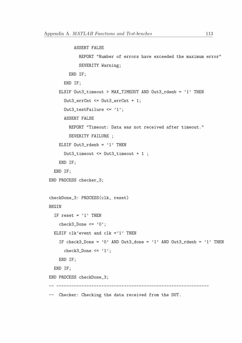
Appendix A. MATLAB Functions and Test-benches 113
ASSERT FALSE
REPORT "Number of errors have exceeded the maximum error"
SEVERITY Warning;
END IF;
END IF;
ELSIF Out3_timeout > MAX_TIMEOUT AND Out3_rdenb = ’1’ THEN
Out3_errCnt <= Out3_errCnt + 1;
Out3_testFailure <= ’1’;
ASSERT FALSE
REPORT "Timeout: Data was not received after timeout."
SEVERITY FAILURE ;
ELSIF Out3_rdenb = ’1’ THEN
Out3_timeout <= Out3_timeout + 1 ;
END IF;
END IF;
END PROCESS checker_3;
checkDone_3: PROCESS(clk, reset)
BEGIN
IF reset = ’1’ THEN
check3_Done <= ’0’;
ELSIF clk’event and clk =’1’ THEN
IF check3_Done = ’0’ AND Out3_done = ’1’ AND Out3_rdenb = ’1’ THEN
check3_Done <= ’1’;
END IF;
END IF;
END PROCESS checkDone_3;
-- -------------------------------------------------------------
-- Checker: Checking the data received from the DUT.
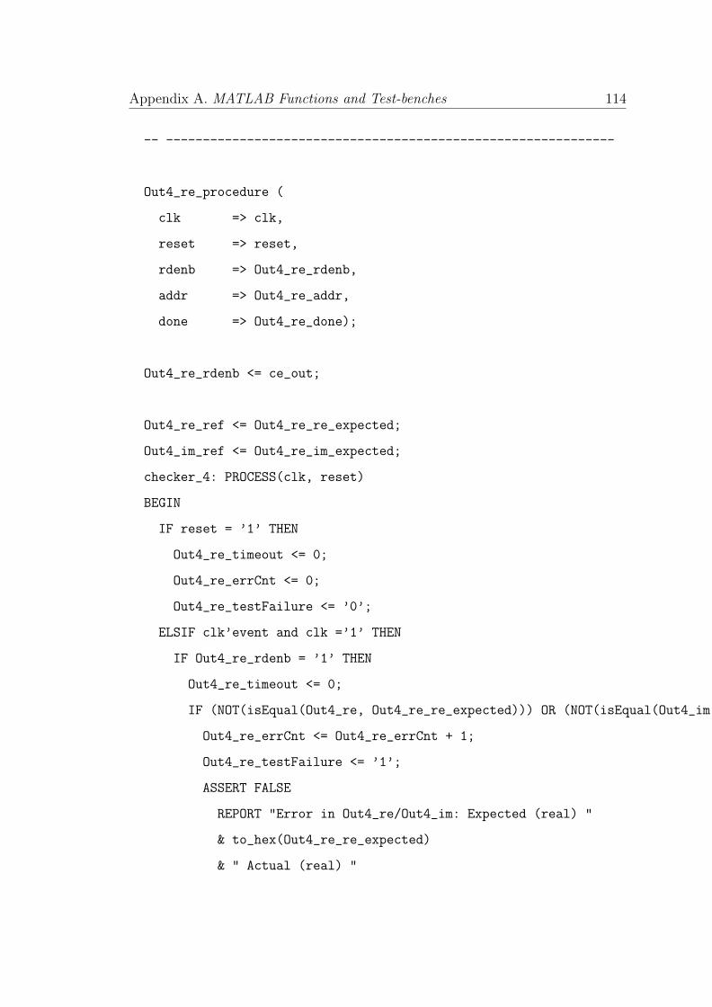
Appendix A. MATLAB Functions and Test-benches 114
-- -------------------------------------------------------------
Out4_re_procedure (
clk => clk,
reset => reset,
rdenb => Out4_re_rdenb,
addr => Out4_re_addr,
done => Out4_re_done);
Out4_re_rdenb <= ce_out;
Out4_re_ref <= Out4_re_re_expected;
Out4_im_ref <= Out4_re_im_expected;
checker_4: PROCESS(clk, reset)
BEGIN
IF reset = ’1’ THEN
Out4_re_timeout <= 0;
Out4_re_errCnt <= 0;
Out4_re_testFailure <= ’0’;
ELSIF clk’event and clk =’1’ THEN
IF Out4_re_rdenb = ’1’ THEN
Out4_re_timeout <= 0;
IF (NOT(isEqual(Out4_re, Out4_re_re_expected))) OR (NOT(isEqual(Out4_im, Out4_re_im_expected))) THEN
Out4_re_errCnt <= Out4_re_errCnt + 1;
Out4_re_testFailure <= ’1’;
ASSERT FALSE
REPORT "Error in Out4_re/Out4_im: Expected (real) "
& to_hex(Out4_re_re_expected)
& " Actual (real) "

Appendix A. MATLAB Functions and Test-benches 115
& to_hex(Out4_re)
& " Expected (imaginary) "
& to_hex(Out4_re_im_expected)
& " Actual (imaginary) "
& to_hex(Out4_im)
SEVERITY ERROR;
IF Out4_re_errCnt >= MAX_ERROR_COUNT THEN
ASSERT FALSE
REPORT "Number of errors have exceeded the maximum error"
SEVERITY Warning;
END IF;
END IF;
ELSIF Out4_re_timeout > MAX_TIMEOUT AND Out4_re_rdenb = ’1’ THEN
Out4_re_errCnt <= Out4_re_errCnt + 1;
Out4_re_testFailure <= ’1’;
ASSERT FALSE
REPORT "Timeout: Data was not received after timeout."
SEVERITY FAILURE ;
ELSIF Out4_re_rdenb = ’1’ THEN
Out4_re_timeout <= Out4_re_timeout + 1 ;
END IF;
END IF;
END PROCESS checker_4;
checkDone_4: PROCESS(clk, reset)
BEGIN
IF reset = ’1’ THEN
check4_Done <= ’0’;
ELSIF clk’event and clk =’1’ THEN

Appendix A. MATLAB Functions and Test-benches 116
IF check4_Done = ’0’ AND Out4_re_done = ’1’ AND Out4_re_rdenb = ’1’ THEN
check4_Done <= ’1’;
END IF;
END IF;
END PROCESS checkDone_4;
-- -------------------------------------------------------------
-- Create done and test failure signal for output data
-- -------------------------------------------------------------
snkDone <= check1_Done AND check2_Done AND check3_Done AND check4_Done;
testFailure <= Out1_testFailure OR Out2_re_testFailure OR Out3_testFailure OR Out4_re_testFailure;
-- -------------------------------------------------------------
-- Global clock enable
-- -------------------------------------------------------------
clk_enable <= tbenb_dly AFTER clk_hold WHEN snkDone = ’0’ ELSE
’0’ AFTER clk_hold;
-- Assignment Statements
END rtl;
Bibliography
[1] Yuan-Chu Yu and Yuan-Tse Yu. Design of a high efficiency reconfigurable
pipeline processor on next generation portable device. In Digital Signal Pro-
cessing and Signal Processing Education Meeting (DSP/SPE), 2013 IEEE,
pages 42–47, Aug 2013. doi: 10.1109/DSP-SPE.2013.6642562.
[2] E. Tell, O. Seger, and D. Liu. A converged hardware solution for fft, dct and
walsh transform. In Signal Processing and Its Applications, 2003. Proceedings.
Seventh International Symposium on, volume 1, pages 609–612 vol.1, July
2003. doi: 10.1109/ISSPA.2003.1224777.
[3] Shousheng He and M. Torkelson. A new approach to pipeline fft processor.
In Parallel Processing Symposium, 1996., Proceedings of IPPS ’96, The 10th
International, pages 766–770, Apr 1996. doi: 10.1109/IPPS.1996.508145.
[4] Chin-Teng Lin, Yuan-Chu Yu, and Lan-Da Van. Cost-effective triple-mode
reconfigurable pipeline fft/ifft/2-d dct processor. Very Large Scale Integration
(VLSI) Systems, IEEE Transactions on, 16(8):1058–1071, Aug 2008. ISSN
1063-8210. doi: 10.1109/TVLSI.2008.2000676.
[5] Chia-Hsiang Yang, Tsung-Han Yu, and D. Markovic. Power and area min-
imization of reconfigurable fft processors: A 3gpp-lte example. Solid-State
Circuits, IEEE Journal of, 47(3):757–768, March 2012. ISSN 0018-9200. doi:
10.1109/JSSC.2011.2176163.
117

Bibliography 118
[6] James W. Cooley and John W. Tukey. An algorithm for the machine calcu-
lation of complex fourier series. Math. Comp.,, 19:297–301, 1965.
[7] K.V. Rangarao and R.K. Mallik. Digital Signal Processing: A Practitioner’s
Approach. Wiley, 2006. ISBN 9780470032879. URL http://books.google.
co.in/books?id=niiudDJK5zIC.
[8] Wen-Chang Yeh and Chein-Wei Jen. High-speed and low-power split-radix
fft. Signal Processing, IEEE Transactions on, 51(3):864–874, March 2003.
ISSN 1053-587X. doi: 10.1109/TSP.2002.806904.
[9] S. Magar, S. Shen, G. Luikuo, M. Fleming, and R. Aguilar. An application
specific dsp chip set for 100 mhz data rates. In Acoustics, Speech, and Sig-
nal Processing, 1988. ICASSP-88., 1988 International Conference on, pages
1989–1992 vol.4, Apr 1988. doi: 10.1109/ICASSP.1988.197015.
[10] J. O’Brien, J. Mather, and B. Holland. A 200 mips single-chip 1 k fft processor.
In Solid-State Circuits Conference, 1989. Digest of Technical Papers. 36th
ISSCC., 1989 IEEE International, pages 166–167, Feb 1989. doi: 10.1109/
ISSCC.1989.48244.
[11] B.M. Baas. A low-power, high-performance, 1024-point fft processor. Solid-
State Circuits, IEEE Journal of, 34(3):380–387, Mar 1999. ISSN 0018-9200.
doi: 10.1109/4.748190.
[12] Guichang Zhong, Fan Xu, and Jr. Willson, A.N. A power-scalable re-
configurable fft/ifft ic based on a multi-processor ring. Solid-State Cir-
cuits, IEEE Journal of, 41(2):483–495, Feb 2006. ISSN 0018-9200. doi:
10.1109/JSSC.2005.862344.
[13] Yu-Wei Lin, Hsuan-Yu Liu, and Chen-Yi Lee. A 1-gs/s fft/ifft processor for
uwb applications. Solid-State Circuits, IEEE Journal of, 40(8):1726–1735,
Aug 2005. ISSN 0018-9200. doi: 10.1109/JSSC.2005.852007.

Bibliography 119
[14] Yuan Chen, Yu-Chi Tsao, Yu-Wei Lin, Chin-Hung Lin, and Chen-Yi Lee.
An indexed-scaling pipelined fft processor for ofdm-based wpan applications.
Circuits and Systems II: Express Briefs, IEEE Transactions on, 55(2):146–
150, Feb 2008. ISSN 1549-7747. doi: 10.1109/TCSII.2007.910771.
[15] Y.-T. Lin, P.-Y. Tsai, and T.-D. Chiueh. Low-power variable-length fast
fourier transform processor. Computers and Digital Techniques, IEE Pro-
ceedings -, 152(4):499–506, July 2005. ISSN 1350-2387. doi: 10.1049/ip-cdt:
20041224.
[16] I. J. Good. ‘the interaction algorithm and practical fourier analysis. Journal
of the Royal Statistical Society, 20(2):361–372, 1958.
[17] W.H. Press. Numerical Recipes 3rd Edition: The Art of Scientific Com-
puting. Cambridge University Press, 2007. ISBN 9780521880688. URL
http://books.google.co.in/books?id=1aAOdzK3FegC.
[18] C. Sidney Burrus. Multidimensional index mapping, May 2012. URL http:
//cnx.org/contents/3c48e4b5-0786-4d1f-bd30-a0cd860be3ab@12.
[19] R. Pratap. Getting Started with MATLAB 7: A Quick Introduction for Sci-
entists and Engineers, chapter Programming in MATLAB:Scripts and Func-
tions, pages 87–115. Oxford University Press, 2006.
[20] Dimitris G. Manolakis John G. Proakis. Digital Signal Processing, chapter
Efficient Computation of the DFT: Fast Fourier Transform Algorithms, pages
511–536. Pearson Prentice Hall, 2007, 2007.
[21] Shravankumar Parunandula, Srujan Gaddam, and Sanath kumar G. A New
Approach to Design and Implement FFT / IFFT Processor Based on Radix-
42 Algorithm. 09 2014. URL http://dx.doi.org/10.6084/m9.figshare.
1183541.
Related Documents