A Na¨ ıve Time Analysis and its Theory of Cost Equivalence DAVID SANDS, DIKU, Department of Computer Science, University of Copenhagen, Universitetsparken 1, DK-2100 Copenhagen, Denmark. E-mail: [email protected] Abstract Techniques for reasoning about extensional properties of functional programs are well understood, but methods for analysing the underlying intensional or operational properties have been much neglected. This paper begins with the development of a simple but useful calculus for time analysis of non-strict functional programs with lazy lists. One limitation of this basic calculus is that the ordinary equational reasoning on functional programs is not valid. In order to buy back some of these equational properties we develop a non-standard operational equivalence relation called cost equivalence, by considering the number of computation steps as an ‘observable’ component of the evaluation process. We define this relation by analogy with Park’s definition of bisimulation in CCS. This formulation allows us to show that cost equivalence is a contextual congruence (and thus is substitutive with respect to the basic calculus) and provides useful proof techniques for establishing cost-equivalence laws. It is shown that basic evaluation time can be derived by demonstrating a certain form of cost equivalence, and we give an axiomatization of cost equivalence which is complete with respect to this application. This shows that cost equivalence subsumes the basic calculus. Finally we show how a new operational interpretation of evaluation demands can be used to provide a smooth interface between this time analysis and more compositional approaches, retaining the advantages of both. Keywords: Time analysis, lazy evaluation, operational semantics. 1 Introduction An appealing property of functional programming languages is the ease with which the extensional properties of a program can be understood—above all the ability to show that operations on programs preserve meaning. Prominent in the study of algorithms in general, and central to formal activities such as program transformation and parallelization, are questions of efficiency, i.e. the running-time and space requirements of programs. These are intensional properties of a program—properties of how the program computes, rather that what it computes. The study of intensional properties is not immediately amenable to the algebraic methods with which extensional properties are so readily explored. Moreover, the declarative emphasis of functional programs, together with some of the features that afford expressive power and modularity, namely higher-order functions and lazy evaluation, serve to make intensional properties more opaque. In spite of this, relatively little attention has been given to the development of methods for reasoning about the computational cost of functional programs. As a motivating example consider the following defining equations for insertion sort (written in a Haskell-like syntax) J. Logic Computat., Vol. 5 No. 93-19:?, pp. 1–46 1995 c Oxford University Press

Welcome message from author
This document is posted to help you gain knowledge. Please leave a comment to let me know what you think about it! Share it to your friends and learn new things together.
Transcript

A Naıve Time Analysis and its Theory ofCost EquivalenceDAVID SANDS, DIKU, Department of Computer Science, University ofCopenhagen, Universitetsparken 1, DK-2100 Copenhagen, Denmark.E-mail: [email protected]
AbstractTechniques for reasoning about extensional properties of functional programs are well understood, but methods foranalysing the underlying intensional or operational properties have been much neglected. This paper begins with thedevelopment of a simple but useful calculus for time analysis of non-strict functional programs with lazy lists. Onelimitation of this basic calculus is that the ordinary equational reasoning on functional programs is not valid. In orderto buy back some of these equational properties we develop a non-standard operational equivalence relation called costequivalence, by considering the number of computation steps as an ‘observable’ component of the evaluation process.We define this relation by analogy with Park’s definition of bisimulation in CCS. This formulation allows us to showthat cost equivalence is a contextual congruence (and thus is substitutive with respect to the basic calculus) and providesuseful proof techniques for establishing cost-equivalence laws. It is shown that basic evaluation time can be derived bydemonstrating a certain form of cost equivalence, and we give an axiomatization of cost equivalence which is completewith respect to this application. This shows that cost equivalence subsumes the basic calculus. Finally we show how anew operational interpretation of evaluation demands can be used to provide a smooth interface between this time analysisand more compositional approaches, retaining the advantages of both.
Keywords: Time analysis, lazy evaluation, operational semantics.
1 IntroductionAn appealing property of functional programming languages is the ease with which the extensionalproperties of a program can be understood—above all the ability to show that operations onprograms preserve meaning. Prominent in the study of algorithms in general, and central toformal activities such as program transformation and parallelization, are questions of efficiency,i.e. the running-time and space requirements of programs. These are intensional propertiesof a program—properties of how the program computes, rather that what it computes. Thestudy of intensional properties is not immediately amenable to the algebraic methods with whichextensional properties are so readily explored. Moreover, the declarative emphasis of functionalprograms, together with some of the features that afford expressive power and modularity, namelyhigher-order functions and lazy evaluation, serve to make intensional properties more opaque. Inspite of this, relatively little attention has been given to the development of methods for reasoningabout the computational cost of functional programs.
As a motivating example consider the following defining equations for insertion sort (writtenin a Haskell-like syntax)
J. Logic Computat., Vol. 5 No. 93-19:?, pp. 1–46 1995 c�
Oxford University Press

2 A Naıve Time Analysis and its Theory of Cost Equivalence
isort [ ] = [ ]isort (h:t) = insert h (isort t)
insert x [ ] = [x]insert x (h:t) = x:(h:t) if �����
= h:(insert x t) otherwise.
As expected, isort requires ������ time to sort a list of length . However, under lazy evaluation,isort enjoys a rather nice modularity property with respect to time: if we specify a program whichcomputes the minimum of a list of numbers, by taking the head of the sorted list, �
minimum � head � isort
then the time to compute minimum is only ����� . This rather pleasing property of insertion-sortis a well-used example in the context of reasoning about running time of lazy evaluation.
By contrast, the following time property of lazy ‘quicksort’ is seldom reported. A typicaldefinition of a functional quicksort over lists might be:
qsort [ ] = [ ]qsort (h:t) = qsort (below h t) ++ (h:qsort (above h t))
where below and above return lists of elements from t which are no bigger, and strictly smallerthan h, respectively, and ��� is infix list-append. Functional accounts of quicksort are alsoquadratic time algorithms, but conventional wisdom would label quicksort as a better algorithmthan insertion-sort because of its better average-case behaviour. A rather less pleasing propertyof lazy evaluation is that by replacing ‘better’ sorting algorithm qsort for isort in the definition ofminimum, we obtain an asymptotically worse algorithm, namely one which is ������ in the lengthof the input.
1.1 Overview
In the first part of the paper we consider the problem of reasoning about evaluation time in termsof a very simple measure of evaluation cost. A simple set of time rules are derived very directlyfrom a call-by-name operational model, and concern equations on ����� � (the ‘time’ to evaluateexpression � to (weak) head normal form) and �����"! (the time to evaluate � to normal-form). Theapproach is naıve in the sense that it is non-compositional (in general, the cost of computing anexpression is not defined as a combination of the costs of computing its subexpressions), and doesnot model graph reduction. However, despite (or perhaps because of) its simplicity, the methodappears to be useful as a means of formalizing sufficiently many operational details to reason(rigorously, but not necessarily formally) about the complexity of lazy algorithms.
One of the principal limitations of the approach is the fact that the usual meanings of ‘equality’for programs do not provide equational reasoning in the context of the time rules. This problemmotivates development of a non-standard theory of operational equivalence in which the numberof computation steps are viewed as an ‘observable’ component of the evaluation process. We#
The example is originally due to D. Turner; it appears as an exercise in informal reasoning about lazy evaluation in [6][Ch. 6], and in the majority(!) ofpapers on time analysis of non-strict evaluation.
A Naıve Time Analysis and its Theory of Cost Equivalence 3
define this relation by analogy with Park’s definition of bisimulation between processes. Thisformulation provides a uniform method for establishing cost-equivalence laws, and together withthe key result that cost equivalence is a contextual congruence, provides a useful substitutiveequivalence with which the time rules can be extended, since if � � is cost equivalent to � � , thenfor any syntactic context $ , �%$�&'� �)( �*��+�%$�&'� �"( �* .
In addition we show that the theory of cost equivalence subsumes the time rules, by providingan axiomatization of cost equivalence which is sound and complete (in a certain sense) withrespect to simple evaluation time properties of expressions.
Finally, we return to a significant flaw in the time model, namely of its use of call-by-namerather than call-by-need. We sketch a method to alleviate this problem which provides a smoothintegration of the simple time analysis here, and the more compositional call-by-need approaches,with some of the advantages of both.
The development of the theory of cost equivalence is somewhat technical, but the paper iswritten so that the reader interested primarily in the problem of time analysis of programs in alazy language should be able to skip the bulk of the technical development, but still take advantageof its results, namely cost equivalence. In the remainder of this introduction we summarize therest of the paper.
Sections 2 to 5 develop a simple time analysis for a first order language with lazy lists. Sec-tion 2 gives some background describing approaches to the efficiency analysis of lazy functionalprograms. In Section 3 we define our language and its operational semantics. Section 4 definesthe notion of time cost over this operational model, and introduces the time rules which form thebasis of the calculus. Section 5 provides some examples of the use of the time rules in reasoningabout the complexity of simple programs.
Section 6 motivates and develops the theory of cost equivalence. Cost equivalence is basedupon a cost simulation preordering which is shown to be preserved by substitution into arbitraryprogram contexts. It is also shown that it is the largest such relation. Section 7 gives somevariants of the co-induction proof principal which are useful for establishing cost equivalences,and presents an axiomatization of cost equivalence which is complete with respect to the basictime properties of expressions. In Section 8 we extend the language with higher-order functions.Time rules are easily added to the new language, and the theory of cost equivalence is extendedin the obvious way by considering an ‘applicative’ cost simulation, which is also shown to havethe necessary substitutivity property.
Section 9 presents an example time analysis, illustrating the combined use of time rules andcost equivalences.
Section 10 outlines a flexible approach to increasing the compositionality and accuracy of thetime analysis with respect to call-by-need evaluation, via the definition of a family of evaluatorsindexed by representations of strictness properties.
To conclude, we consider related work in the area of intensional semantics.
A preliminary version of this paper appeared as [39], and summarized [36][Ch. 4]. In additionto the inclusion of proofs, further examples and additional technical results, Sections 7, 8, 9 and10 are new, and contain a number of important extensions to the earlier work.
2 Time analysis: backgroundA number of researchers have developed prototype (time) complexity analysis tools in which thealgorithm under analysis is expressed as a first-order call-by-value functional program [44, 22,

4 A Naıve Time Analysis and its Theory of Cost Equivalence
33, 17]. It could be argued that the subject of study in these cases is not functional programmingper se; the choice of a functional language is motivated by the fact that, for a first-order languagewith a call-by-value semantics, it is straightforward to construct, mechanically, functions with thesame domain as a given function, which describe (recursively) the number of computation stepsrequired by that function. Although this does not by any means trivialize the problem of findingsolutions to these equations in terms of some size-measure of the arguments, it gives a simple butformal reading of the program as a description of computational cost. This is because the cost ofevaluating some function application fun( , ) can be understood in terms of the cost of evaluating, , plus the cost of evaluating the application of fun to the value of , .
In the case of a higher-order strict language cost is not only dependent on the simple cost ofevaluating the argument , , but also on the possible cost of subsequently applying , , applyingthe result of an application, and so forth. Techniques for handling this problem were introducedin [34], where syntactic structures called cost closures were introduced to enable intensionalproperties to be carried by functions. Additional techniques for reasoning about higher-orderfunctions which complement this approach are described in [36].
A problem in reasoning about the efficiency of programs under lazy evaluation (i.e. call-by-name, or more usually, call-by-need, extended to data structures) is that the cost of computing thesubexpression , is dependent entirely on the way in which the expression is used in the functionfun. More generally, the cost of evaluating some (sub)expression is dependent on the amount ofits value needed by its context.
The compositional approachOne approach to reasoning about the time cost of lazy evaluation is to parameterize the descriptionof the cost of computing an expressionby a description of the amount of the result that is needed bythe context in which it appears. This approach is due to Bjerner [7], where a compositional theoryfor time analysis of the (primitive recursive) programs of Martin-Lof type-theory is developed.A characterization of ‘need’ (more accurately ‘not-need’) provided by a new form of strictnessanalysis [43] enabled Wadler to give a simpler account of Bjerner’s approach [42] in the contextof a (general) first-order functional language. The strictness-analysis perspective also gives anatural notion of approximation in the description of context information, and gives rise, viaabstract interpretation to a completely mechanizable analysis for reasoning about (approximate)contexts. In [37, 36] the context information available from such an analysis is used to characterizesufficient-time and necessary-time equations which together provide bounds on the exact timecost of lazy evaluation, and the method is extended to higher-order functions using a modificationof the cost-closure technique.
A problem with these compositional approaches to time analysis remains: the informationrequired about context is itself an uncomputable property in general. The options are to settleeither for approximate information via abstract interpretation (or a related approach), or towork with a complete calculus for contexts and hope to find more exact solutions. The formerapproach, while simplifying the task of reasoning about context (assuming that an implementationis available), can lead to unacceptable approximations in time cost. The latter approach (see [8])can be impractically cumbersome for many relatively simple problems, and is unlikely to extendusefully to higher-order languages.

A Naıve Time Analysis and its Theory of Cost Equivalence 5
The naıve approachIn the following three sections, we explore a complementary approach which begins with a moredirect operational viewpoint. We define a small first-order lazy functional language with lists, anddefine time cost in terms of an operational model. (The treatment of a higher-order language inthe naıve approach is just as straightforward, but is postponed in order to simplify the expositionof the theory of cost equivalence.) The simplicity of the chosen semantics (a substitution-basedcall-by-name model) leads to a correspondingly straightforward definition of time cost, which isrefined to give an unsophisticated calculus, in the form of time rules with which we can analysetime cost. We illustrate the utility of the naıve approach before going on to consider extensionsand improvements.
3 A simple operational modelWe initially consider a first-order language with lists. For simplicity we present an untypedsemantics, but the syntax will be suggestive of a typed version. List construction is sugared withan infix cons ‘:’, and lists are examined and decomposed via a case-expression. Programs areclosed expressions in the context of function definitions-�. ��/ �10�2�2�2"0 /43657 8��� . 2We also assume some strict primitive functions over the atomic constants of the language(booleans, integers etc.). Expressions are described by the grammar in Fig. 1.� 979'� - �� � 0�2�2�2 0 � 3 (function call): ; �� � 0�2�2�2)0 � 3 (primitive function call):
if � � then � � else �=< (conditional): >?case � � of
nil @A� �/B9C/ED�@A� < FG(list-case expression): � � 9H� � (cons): / (identifier): I(constant)
FIG. 1. Expression syntax
3.1 Semantic rules
It is possible to reason about time-complexity of a closed expression by reasoning directlyabout the ‘steps’ in the evaluation of an expression. The problem with this approach is that itrequires us to have the machinery of an operational semantics at our fingertips in order to reasonin a formal manner. The degree of operational reasoning necessary can be minimized by anappropriately abstract choice of semantics. In particular, simplicity motivates the choice of acall-by-name calling mechanism—shortcomings and improvements to this model are discussedin Section 10. The semantics is defined via two types of evaluation rule: one describing evaluationto head-normal-form, and one for evaluation to normal-form. Including rules for evaluation to

6 A Naıve Time Analysis and its Theory of Cost Equivalence
normal-form is somewhat non-standard for the semantics of a lazy language. To talk aboutthe complete evaluation of programs it is usual to define a print-loop to describe accurately thetop-level behaviour of a program. Since our motivation is the analysis of time cost, the rules forevaluation to normal-form give a convenient approximation to the printing mechanism (since inthe case of non-terminating programs we would need to place them in some ‘terminating context’to describe their time behaviour anyway).
Fun� . J � �LK / �NM�M�M � 3 5 K / 3 5�OQPBRQS- . ��� � 0�2�2�2"0 � 3 5T 8PBR�S
Prim� � PBU I �VM�M�M � 3XW PBU ILY ��Z[� apply\4� ; . 0 I � 0�2�2�2 0 I 3 5% ) ; . ��� � 0�2�2�2"0 � 3]W ^P_R�Z
Cond� � PBU true � � PBR�S
if � � then � � else �=<QPBR�S � � P U false � < P R Sif � � then � � else �L<`PBR�S
Cons� � PBabZ �`0 � � PBaBZ �� � 9H� � P a Z � 9CZ � � � 9C� � P U � � 9C� �
Const I P R ICase
� � PBU nil � � P_R�S>?case � � of
nil @c� �/B9C/ED�@c� < FG P R S � � PBUB��de9C�=fg�=< J ��d K / 0 �=f K /hDiO`PBR�S>?case � � of
nil @c� �/B9H/ED�@c�=< FG P_R�SFIG. 2. Dynamic semantics
We define the operational semantics via rules which allow us to make judgements of the form:��PBajZ and ��P Ulk . These can be read as ‘expression � evaluates to normal form Z ’ and‘expression � evaluates to head-normal form � k ’ respectively. There is no rule for evaluating avariable—evaluation is only defined over closed expressions. These rules are presented in Fig. 2,using meta-variable m to range over labels n and o . Normal-forms, ranged over by Z 0 Z � 0 Z �etc. (sometimes referred to simply as values) are the fully evaluated expressions i.e. either fullyevaluated lists, or atomic constants (
I): Z�979'� I[: Z � 9CZ �H2
Head-normal forms, ranged over by k 0 k � 0 k � etc., are simply the constants and arbitrary cons-expressions: k 979 � I[: � � 9H� � 2
A brief explanation of the semantic rules is given below:pThe use of the term head-normal-form is not to be confused with the corresponding notion in the (pure) lambda calculus; we use this term as a first-order
manifestationof the notion of weak head-normal-form from the terminology of lazy functional languages [31].

A Naıve Time Analysis and its Theory of Cost Equivalence 7q To describe function application we perform direct substitution of parameters. We use thenotation � J �=r K /�O to mean expression � with free occurrences of / replaced by the expression� r (see comments below).q We assume the primitive functions are strict functions on constants, and are given meaningby some partial function apply \ . Since the constants are included in the head-normal formsis it sufficient to evaluate the arguments to primitive functions with PsU . In a lower-levelsemantics in which errors (eg. ‘divide-by-zero’) are distinguished from non-termination thischoice would be significant, but here it makes no difference.q To evaluate a case-expressioneither to normal or head-normal-form, we must evaluate the list-expression � � to determine which branch to take. However, we do not evaluate the expressionany further than the first cons-node.
NotationWe summarize some of the notation used in the remainder of the paper.
Variables and substitution A list of zero or more variables / � 0�2�2�2 / 3 will often be denoted t/ ,and similarly for a list of expressions.
We use the notation � J � � 0�2�2�2"0 � 3 K / � 0�2�2�2"0 / 3 O to mean expression � with free occurrences of/ � 0�2�2�2"0 / 3 simultaneously replaced by the expressions � � 0�2�2�2u0 � 3 . In a case expression
case � � ofnil @v� �/B9C/hDN@v� <
the variables / and /hD are considered bound in � < . A formal definition of substitution is omitted,but is standard (see e.g. [4]). We will also assume the following substitution property (the standard‘substitution lemma’): if variables t/ and tw are distinct, then; J tx K t/�O J ty K tw O`� ; J ty K tw O J tx J ty K tw O K t/hOwhere tx J ty K tw OQ� x � J ty K tw O 0�2�2�2 0 x 3 J ty K tw O
The idea of a context, ranged over by $ , $ � , etc. will be used (informally) to denote anexpression with a ‘hole’, & ( , in the place of a subexpression; $�& � ( is the expression produced byreplacing the hole with expression � . Generally we will assume that the expression is closed, andso this notation can be considered shorthand for substitution. <Relations If z is a relation, then we will usually write {|z~} to mean ��{ 0 }L ^�Vz . A relation zis a preorder if it is transitive and reflexive, and an equivalence relation if it is also symmetric.Syntactic equivalence up to renaming of bound variables will be denoted � . The maximumrelation on closed expression will be denoted by � .
4 Deriving time-rulesWe wish to reason about the time cost of evaluating an expression. For simplicity we express thisproperty in terms of the number of non-primitive function calls occurring in the evaluation of theexpression.�
Formal definitions usually allow free variables in � to be captured by � . We will revert to the substitution notation when we need to be more formal, andconsider the special case of variable capture explicitly.
8 A Naıve Time Analysis and its Theory of Cost Equivalence
For the operational semantics given, the evaluation process is understood in terms of (theconstruction of) a proof of some judgement according to the semantic rules. The above propertyof an evaluation corresponds to the number of instances of the rule Fun in the proof of ��PsR�Sfor some closed expression � , whenever such a proof exists for some S . In order to extract rulesfor reasoning about this property, we rely on some basic properties of the semantics:q The rules describe deterministic computation: if ��P R S and �`P R S4r then S���S4r .q Proofs are unique: if � and ��r are proofs of ��PBR�S then � and ��r are identical.
In the following let � 0 � � 2�2�2 range over judgements of the form ��PbR�S , and let � 0 � � 2�2�2range over proofs of judgements.
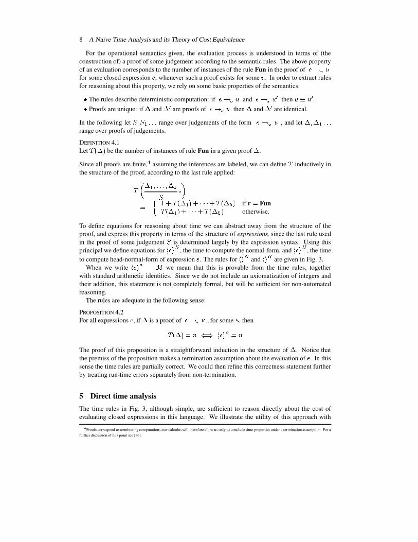
DEFINITION 4.1Let ����� be the number of instances of rule Fun in a given proof � .
Since all proofs are finite, � assuming the inferences are labeled, we can define � inductively inthe structure of the proof, according to the last rule applied:��� � �i0�2�2�2 0 � Y
r� �� ��� ������� � �� M�M�M ������� Y if r � Fun����� � �� M�M�M �l���� Y otherwise 2To define equations for reasoning about time we can abstract away from the structure of theproof, and express this property in terms of the structure of expressions, since the last rule usedin the proof of some judgement � is determined largely by the expression syntax. Using thisprincipal we define equations for �%���u! , the time to compute the normal-form, and �%���"� , the timeto compute head-normal-form of expression � . The rules for �%� ! and �%� � are given in Fig. 3.
When we write �%��� * ��� we mean that this is provable from the time rules, togetherwith standard arithmetic identities. Since we do not include an axiomatization of integers andtheir addition, this statement is not completely formal, but will be sufficient for non-automatedreasoning.
The rules are adequate in the following sense:
PROPOSITION 4.2For all expressions � , if � is a proof of �`P R S , for some S , then����� ���A��@ �%���"*���The proof of this proposition is a straightforward induction in the structure of � . Notice thatthe premiss of the proposition makes a termination assumption about the evaluation of � . In thissense the time rules are partially correct. We could then refine this correctness statement furtherby treating run-time errors separately from non-termination.
5 Direct time analysisThe time rules in Fig. 3, although simple, are sufficient to reason directly about the cost ofevaluating closed expressions in this language. We illustrate the utility of this approach with�
Proofs correspond to terminating computations;our calculus will therefore allow us only to conclude time-propertiesunder a termination assumption. For afurther discussion of this point see [36].
A Naıve Time Analysis and its Theory of Cost Equivalence 9� - . ��� � 0�2�2�2"0 � 3 5� )�"* � � �~��� . J � ��K / � 0�2�2�2"0 � 3 5 K / 3 5�O1� *� ; ��� �10�2�2�2"0 � Y )� * � �%� � � � � M�M�M �~��� Y � �� if � � then � � else � < � * � �%� � ���j� � ��� � �)* if � � PBU true���L<i�)* if � � PBU false�case � � of
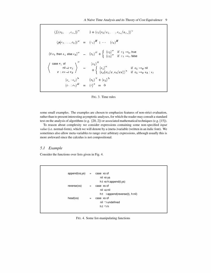
nil @c� �/B9C/ED�@c�=<�� * � �� � � �� � �%� � �)* if � � P_U nil�%�=< J ��d K / 0 �=f K /ED�O1�* if � � P_Us��d�9H�Lf�%� � 9C� � �! � �%� � ��!j� �%� � ��!�%� � 9C� � �� � � I � * � ¡FIG. 3. Time rules
some small examples. The examples are chosen to emphasize features of non-strict evaluation,rather than to present interesting asymptotic analyses, for which the reader may consult a standardtext on the analysis of algorithms (e.g. [20, 2]) or associated mathematical techniques (e.g. [15]).
To reason about complexity we consider expressions containing some non-specified inputvalue (i.e. normal-form), which we will denote by a (meta-)variable (written in an italic font). Wesometimes also allow meta-variables to range over arbitrary expressions, although usually this ismore awkward since the calculus is not compositional.
5.1 Example
Consider the functions over lists given in Fig. 4.
append(xs,ys) = case xs ofnil @ ysh:t @ h:append(t,ys)
reverse(xs) = case xs ofnil @ nilh:t @ append(reverse(t), h:nil)
head(xs) = case xs ofnil @ undefinedh:t @ h
FIG. 4. Some list-manipulating functions

10 A Naıve Time Analysis and its Theory of Cost Equivalence
Now we wish to consider the cost of evaluating the expression
head(reverse( Z ))
which computes the last element of some non-empty list-value Z��¢ZHd~9£Z�f . Applying thedefinitions in Fig. 3 � head(reverse( Z )) � ! � � �~� reverse( Z ) � � ����� d � !where reverse( Z ) PBUb��d�9C�=f for some ��d 0 �Lf . It is not hard to show that ��d is a value (using thefact that Z is, and by induction on its length), and hence that �%� d � ! ��¡ . Now since Z[��Z d 9CZ f ,and hence Z[P U Z d 9HZ f we have that� reverse( Z ) � �� � ���%ZC� � �~� append(reverse( Z�f ), Z�d :nil) � �� � ��� append(reverse( Z f ), Z d :nil) ��� � � � �~� reverse( Z1f ) � ��¥¤¦ § � nil ��� 0 if reverse( Z�f ) PBU nil���Lr d 9 append( �Lrf , Zid :nil) �� 0
if reverse( Z1f ) PBUb�Lrd 9C�Lrf� ¨©��� reverse( Z f ) �� 2We now have the recurrence equations parameterized by the input value:� reverse(nil) ��� � �� reverse( Z�9HZCD ) �u� � ¨©��� reverse( ZCD ) � �whose solution is � reverse( Z ) �)�ª� � ��¨C , where is the length of the list Z . Thus we have atotal cost of � head(reverse( Z )) � ! �~¨]� � �j� where is the length of the list Z , i.e. linear time complexity (compare with quadratic complexityfor the call-by-value reading, and for � reverse( Z ) � ! ).
5.2 Example
Here we present the example from the introduction (in the syntax we have defined) which showsthe rather pleasing property that one can compute the smallest element of a list in linear timeby taking the first element of the (insertion-) sort of the list. The equations in Fig. 5 define aninsertion-sort function (isort).
The time to compute the head-normal-form of insertion-sort given some list-value (normal-form) Z is easily calculated from the time rules. First consider the insertion function. Anyexhaustive application of the time rules together with a few minor simplifications allow us toconclude that for integer valued expressions � � , and integer-list valued expressions � � ,� insert( � � , � � ) � � � � �~�� � � ���� ¡ if � � PBU nil�%� � � � � � k � � if }©PBU k 9�« 2

A Naıve Time Analysis and its Theory of Cost Equivalence 11
isort(xs) = case xs ofnil @ nilh:t @ insert(h, isort(t))
insert(x, ys) = case ys ofnil @ x:nilh:t @ if x � h
then x:(h:t)else h:insert(x,t)
FIG. 5. Insertion sort
Now consider computing the head-normal-form of insertion-sort applied to some list of integersZ 3 9 2�2�2 9CZ � 9 nil where b¬ � . To aid notation, let 4® denote the list nil and, for each ¯^°~ , let .�± � denote the list Z .�± � 9] . . � isort( ® ) ���� �� isort( .�±h. ) ���� � ��� insert( Z .�± � ,isort( . )) � �� � � � �~� isort( . ) ���+ � ¡ if isort( . ) PBU nil��Z .T± � ����~� k ��� if isort( . ) PBU k 91« 2
Clearly �%Z .�± � � � �²¡ . A simple induction in ¯ establishes that if isort( . ) P_U k 9�« then� k � � ��¡ also. This leaves us with the simple recurrence� isort( 6® ) � � � �� isort( .T±h. ) ��� � ¨©� � isort( . ) ��giving � isort( 3 ) � � ��¨H|� � .
5.3 Example
Consider the following (somewhat non-standard ³ ) definition of Fibonacci:
fib(n) = f(n,0)f(n, r) = if n=0 then 1
else r + f(n-1, f(n-2,0)).´
Note that under a call-by-value semantics fib is divergent for any n µ`¶ .
12 A Naıve Time Analysis and its Theory of Cost Equivalence
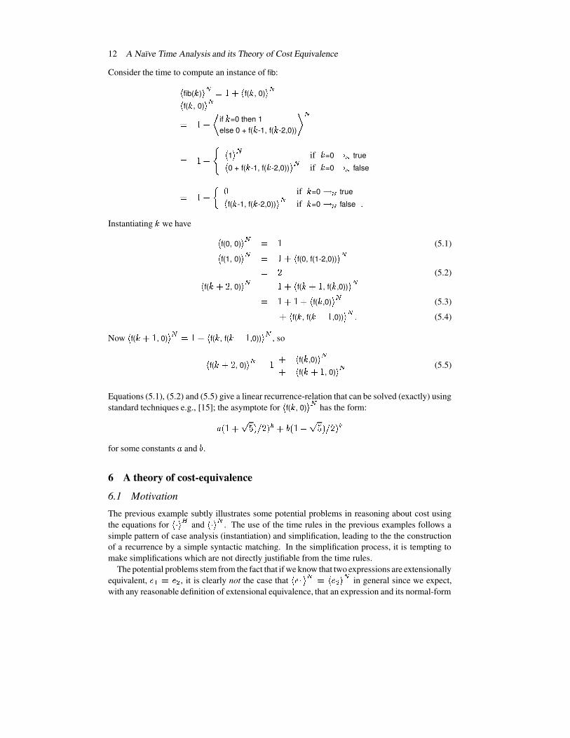
Consider the time to compute an instance of fib:� fib( · ) �!�� � �~� f( · , 0) � !� f( · , 0) � !� � ��¸ if · =0 then 1else 0 + f( · -1, f( · -2,0)) ¹ !
� � ��º � 1 �! if · =0 P a true� 0 + f( · -1, f( · -2,0)) ��! if · =0 PBa false� � � � ¡ if · =0 P a true� f( · -1, f( · -2,0)) �u! if · =0 PBa false 2Instantiating · we have � f(0, 0) �! � � (5.1)� f(1, 0) �! � � ��� f(0, f(1-2,0)) ��!� ¨ (5.2)� f( ·[��¨ , 0) � ! � � ��� f( ·[� � , f( · ,0)) � !� � � � ��� f( · ,0) ��! (5.3)��� f( · , f( ·¼» � ,0)) ��! 2 (5.4)
Now � f( ·[� � , 0) �!�� � � � f( · , f( ·�» � ,0)) ��! , so� f( ·[�l¨ , 0) � ! � � � � f( · ,0) ��!� � f( ·[� � , 0) � ! 2 (5.5)
Equations (5.1), (5.2) and (5.5) give a linear recurrence-relation that can be solved (exactly) usingstandard techniques e.g., [15]; the asymptote for � f( · , 0) � ! has the form:{4� � ��½ ¾C K ¨C Y ��}�� � »¿½ ¾H K ¨H Yfor some constants { and } .6 A theory of cost-equivalence
6.1 Motivation
The previous example subtly illustrates some potential problems in reasoning about cost usingthe equations for � M � � and � M � ! . The use of the time rules in the previous examples follows asimple pattern of case analysis (instantiation) and simplification, leading to the the constructionof a recurrence by a simple syntactic matching. In the simplification process, it is tempting tomake simplifications which are not directly justifiable from the time rules.
The potential problems stem from the fact that if we know that two expressions are extensionallyequivalent, � � �À� � , it is clearly not the case that �%� � �!A�v�%� � �! in general since we expect,with any reasonable definition of extensional equivalence, that an expression and its normal-form

A Naıve Time Analysis and its Theory of Cost Equivalence 13
(supposing one exists) will be equivalent. More generally given any context $ , we expect that$�&'� �( ��$�&'� � ( , but not that �%$�&'� ��( � * �À�$�&'� � ( � * in general, so ordinary equational reasoningis not valid within the time rules. Similarly if ��� � ����À�%� � �� then we cannot expect in generalthat ��$�& � �( �����+�%$�& � � ( �� .
However, even in the last example above we have used simple equalities such as (line 5.4)�·�� � - 1 ��· in precisely this way (albeit benignly) to simplify cost expressions in orderto construct a recurrence. Á In this instance the simplification is obviously correct, but with thecurrent calculus we cannot justify it.
To take a less contrived example, where the limitations of the method are more significant,consider the quicksort program given in the introduction. The following equations (Fig. 6) definea simple functional version of quicksort (qs) using auxiliary functions below and above, andappend (as defined earlier) written here as an infix function ��� . Primitive functions for integercomparison have also been written infix to aid readability. The definition for above has beenomitted, but is like that of below with the comparison ‘  ’ in place of ‘ � ’.
qs(xs) = case xs ofnil @ nilh:t @ qs(below(h,t))��� (h : qs(above(h,t)))
below(x,ys) = case ys ofnil @ nilh:t @ if h � x then h : below(x,t)
else below(x,t)
FIG. 6. Functional quicksort
The aim will be fairly modest: to show that quicksort exhibits its worst-case ������� behavioureven when we only require the first element of the list to be computed, in contrast to the earlierinsertion sort example which always takes linear time to compute the first element of the result.First consider the general case:� qs( � ) � � � � �~����� � �ä¦ § ¡ if �`PBU nil¸ qs(below( w , Ä ))��� ( w :qs(above( w , Ä ))) 2 ¹ �
if �`PBU w : ÄFrom the time rules and the definition of append, this simplifies to� qs( � ) ���� � �~����� �l� � ¡ if �©PBU nil� �~� qs(below( w , Ä )) ��� if �©P U w : Ä 2 (6.1)
Proceeding to the particular problem, it is not too surprising that we will use non-increasinglists Z to show that � qs( Z ) � � �Å������� . Towards this goal, fix an arbitrary family of integerÆ
Spelling this simplificationout, we have an applicationof a primitive function (subtraction) to the (meta) constant ‘ ÇhÈÊÉ ’ (i.e., the constant one larger thanthe meta-constant Ç ), which we simplify to ‘ Ç ’.

14 A Naıve Time Analysis and its Theory of Cost Equivalence
valuesJ Z . O .%Ë ® such that Z . �ÌZ"Í whenever ¯Î��Ï . Now define the family of non-increasing listsJ�Ð`. O .%Ñ ® by induction on ¯ : Ð ®Ò� nilÐ Y ± � � Z Y ± � 9 Ð Y 2
The goal is now to show that � qs(Ð 3 ) � � is quadratic in . Instantiating the general equation (6.1)
in the ‘interesting’ case when ��� Ð Y ± � for some ·e¬~¡ we obtain:� qs(Ð Y ± � ) ���� � �~� Ð Y ± � ���j� � ��� qs(below( w , Ä] ) � �
whereÐ Y ± � P U w : Ä� ¨©�~� qs(below( Z Y ± � ,
Ð Y ± � )) ��� 2At this point we can only further manipulate the expression � qs(below( Z Y ± � ,
Ð Y ± � )) ��� :� qs(below( Z Y ± � ,Ð Y ± � )) � �� � � � below( Z Y ± � ,
Ð Y ± � ) ���� � � � qs(below( w , Ä )) � �where below( Z Y ± � ,
Ð Y ± � ) PBU w : Ä� Ó©� � qs(below( Z Y ± � ,below( Z Y ± � ,Ð Y
))) �� 2So now we have the equation� qs(
Ð Y ± � ) � � � ¾©��� qs(below( Z Y ± � ,below( Z Y ± � ,Ð Y
))) � � 2This should be sufficient to convince the reader that quadratic-time behaviour is a possibility,since in the successive recursive calls to qs (with respect to this time equation) we can see thatthe arguments become increasingly complex, and it becomes increasingly costly to compute theirrespective head-normal-forms.
With the current calculus we can do little more than give this intuition. What we are not ableto do is to simplify or generalize the calls to below to obtain a simple recurrence equation. Wewill return to this example.
The remainder of this section is devoted to developing a stronger notion of equivalence ofexpressions which respects cost, and allows a richer form of equational reasoning on expressionswithin the calculus. We will conclude the above example in Section 7.3.
What is needed is an appropriate characterization of (the weakest) equivalence relation ��ÔÖÕwhich satisfies �`�¼ÔÖÕN� r ��@¥�$�&'� ( �*��×��$�&'�Lr ( � * 2To develop this general ‘contextual congruence’ relation, we use a notion of simulation similar tothe various simulations developed in process algebras such as Milner’s calculus of communicatingsystems [26]. In the theory of concurrency a central idea is that processes that cannot bedistinguished by observation should be identified. This ‘observational’ viewpoint is adopted inthe ‘lazy’ Ø -calculus [1], where an equivalence called applicative bisimulation is introduced. Inthe lazy Ø -calculus, the observable properties are just the convergence of untyped lambda-terms.For our purposes we need to treat cost as an observable component of the evaluation process, andso we develop a suitable notion of cost (bi)simulation.

A Naıve Time Analysis and its Theory of Cost Equivalence 15
6.2 Cost simulation
The partial functions PVU and P a together with ��� ! and �%��� are not sufficient to characterizecompletely the cost behaviour of expressions in all contexts, since we need to characterizepossiblyinfinite ‘observations’ on expressions which arise in our language because of the non-strict list-constructor (c.f. untyped weak head-normal-forms in [1]).
Roughly speaking, the notion of equivalence we want satisfies:� and �Lr are equivalent iff �����u�������Lr�� � and their head-normal-forms are either1. identical constants, or2. cons-expressions, whose corresponding components are equivalent.
Unfortunately, although this is a property that we would like our equivalence to obey, it does notconstitute a definition (to see why, note that we not only wish to relate expressions having normal-forms, but also those which are ‘infinite’), so following [26] we use a technique due to Park [30]for identifying processes—the notion of a bisimulation and its related proof technique. We willdevelop the equivalence relation we require in terms of preorders called cost simulations—wewill then say that two expressions are cost equivalent if they simulate each other.
To simplify our presentation we add some notation:
DEFINITION 6.1If ٠is a binary relation on closed expressions, then ٠9 is the binary relation on head-normal-formssuch that � k ٠9 k r ��@ either k � k rh� I
or k ��� � 9H� � 0 k rE�~�=r � 9C�=r� and� � Ùc�Lr � 0 and � � ÙÛ�=r� 2DEFINITION 6.2The cost-labelled transition,
fP_R , «Ê� N is defined� fP_R�S def.�Ü�`PBR�S and �%��� * ��« 2Now we define a basic notion of cost simulation, by analogy with Park’s (bi)simulation:
DEFINITION 6.3 (Cost Simulation)
A binary relation Ù on closed expressions is a cost simulation if, whenever �^Ùc�1r� fP Ubk ��@��Î� r fP Ubk r and k Ù 9 k r 2DEFINITION 6.4For each relation Ý on closed expressions, define Þe��Ý[ to be the relation on closed expressionsthat relates � and ��r exactly when� fPBU k ��@���� r fPBU k r and k Ý 9 k r 2Now we can easily see thatq Þ is monotonic, i.e., ÙÅßjàl��@áÞe��Ù_ âßjÞe�%àÊ q à is a cost simulation iff à�ß²Þ���àÊ (since à²ß�Þ���àÊ means that ã�� � 0 � � 0 � � �Î� � @� �Lä ��� � � , and by expanding the definition of ä we recover Definition 6.3).
16 A Naıve Time Analysis and its Theory of Cost Equivalence
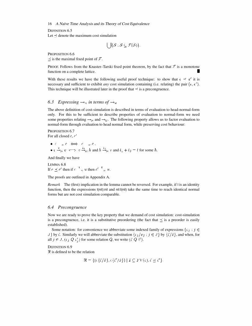
DEFINITION 6.5Let å denote the maximum cost simulationæ J à~9ià�ß�Þ���àÊ "O 2PROPOSITION 6.6å is the maximal fixed point of Þ .
PROOF. Follows from the Knaster–Tarski fixed point theorem, by the fact that Þ is a monotonefunction on a complete lattice.
With these results we have the following useful proof technique: to show that ��å²�1r it isnecessary and sufficient to exhibit any cost simulation containing (i.e. relating) the pair �� 0 �ir� .This technique will be illustrated later in the proof that å is a precongruence.
6.3 Expressing ç�è in terms of ç�éThe above definition of cost-simulation is described in terms of evaluation to head-normal-formonly. For this to be sufficient to describe properties of evaluation to normal-form we needsome properties relating P a and PBU . The following property allows us to factor evaluation tonormal-form through evaluation to head normal form, while preserving cost behaviour:
PROPOSITION 6.7For all closed � , ��rq �`PBa I ��@ ��P U I
.q � fP a Z���@ � f #PBU k and k f pP a Z and « � �ê« � �j« for some k .
And finally we have
LEMMA 6.8If �ëåÌ�=r then if � fP_aBS then �=r fPBabS .
The proofs are outlined in Appendix A.
Remark The (first) implication in the lemma cannot be reversed. For example, if I is an identityfunction, then the expressions I(nil):nil and nil:I(nil) take the same time to reach identical normalforms but are not cost simulation comparable.
6.4 Precongruence
Now we are ready to prove the key property that we demand of cost simulation: cost-simulationis a precongruence, i.e. it is a substitutive preordering (the fact that å is a preorder is easilyestablished).
Some notation: for convenience we abbreviate some indexed family of expressionsJ �LÍ�9iÏ��ì O by í� . Similarly we will abbreviate the substitution
J �"Í K /HÍ[9�Ï�� ì O byJ í� K í/îO , and when, for
all Ï|� ì, ��� Í�Ý��LrÍ for some relation Ý , we write �Lí��ÝÀí�=r7 .
DEFINITION 6.9ïis defined to be the relationï � J ��� J í� K í/�O 0 � J í� r K í/�O1 : í/eß ä [���� 0 í��å�í� r O 2
A Naıve Time Analysis and its Theory of Cost Equivalence 17
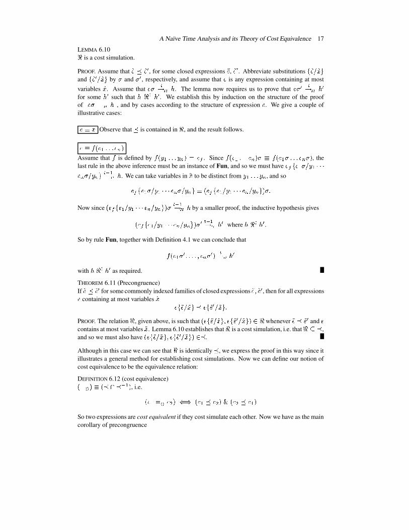
LEMMA 6.10ïis a cost simulation.
PROOF. Assume that í�¼åAí�=r , for some closed expressions í� , í��r . Abbreviate substitutionsJ í� K í/hO
andJ í�=r K í/�O by ð and ðhr , respectively, and assume that � is any expression containing at most
variables í/ . Assume that ��ð fPBU k . The lemma now requires us to prove that ��ðîr fPBU k rfor some k r such that k ï 9 k r . We establish this by induction on the structure of the proofof ��ð�PBU k , and by cases according to the structure of expression � . We give a couple ofillustrative cases:�`�~/ Observe that å is contained in
ï, and the result follows.�`� - ��� � 2�2�2 � 3
Assume that-
is defined by- � w � 2�2�2 w 3 ¼�A�Lñ . Since
- �� � 2�2�2 � 3 ðj� - ��� � ð 2�2�2 � 3 ð� , thelast rule in the above inference must be an instance of Fun, and so we must have �1ñ J � � ð K w ��M�M�M�=3Eð K w 3hO f�ò �P U~k . We can take variables in í/ to be distinct from w ��2�2�2 w 3 , and so�=ñ J � � ð K w ��M�M�M � 3 ð K w 3 Oó�ô���=ñ J � ��K w �NM�M�M � 3 K w 3 Oi )ð 2Now since ���=ñ J � �LK w �NM�M�M � 3 K w 3 O1 )ð fò �P_U k by a smaller proof, the inductive hypothesis gives���=ñ J � ��K w ��M�M�M � 3 K w 3 Oi )ð r f�ò �PBU k r where k ï 9 k r .So by rule Fun, together with Definition 4.1 we can conclude that- ��� � ð r 0�2�2�2"0 � 3 ð r fPBU k rwith k ï 9 k r as required.
THEOREM 6.11 (Precongruence)If í��å�í�Lr for some commonly indexed families of closed expressions í� 0 í��r , then for all expressions� containing at most variables í/ � J í� K í/hO[åj� J í� r K í/hO 2PROOF. The relation
ï, given above, is such that ��� J í� K í/îO 0 � J í��r K í/�O1 ^� ï
whenever í��å�í�=r and �contains at most variables í/ . Lemma 6.10 establishes that
ïis a cost simulation, i.e. that
ï ß�å ,and so we must also have �� J í� K í/�O 0 � J í��r K í/�Oi 8�^å .
Although in this case we can see thatï
is identically å , we express the proof in this way since itillustrates a general method for establishing cost simulations. Now we can define our notion ofcost equivalence to be the equivalence relation:
DEFINITION 6.12 (cost equivalence)��[ÔÖÕ 8�õ�)ålöså ò �� , i.e. �� � � ÔÖÕ � � Ú��@ ��� � å~� � 8÷õ��� � å~� � So two expressions are cost equivalent if they cost simulate each other. Now we have as the maincorollary of precongruence
18 A Naıve Time Analysis and its Theory of Cost Equivalence
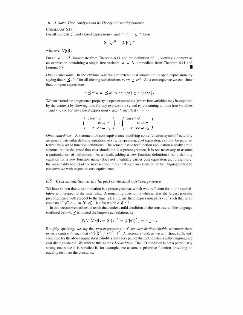
COROLLARY 6.13For all contexts $ , and closed expressions � and ��r , if ���¼ÔÖÕ��=r , then��$�&'� ( � * �+�%$�&'�=r ( � *whenever $�&'� (ùø RPROOF. m��cn , immediate from Theorem 6.11 and the definition of å , viewing a context asan expression containing a single free variable; m��¢o , immediate from Theorem 6.11 andLemma 6.8
Open expressions In the obvious way we can extend cost simulation to open expressions bysaying that ��å��=r if for all closing substitutions ð , ��ðúå���ð�r . As a consequence we can showthat, on open expressions,��å~� r ÷~� � å~� � @û� J � � K /�OQå~� r J � � K /�O 2We can extend the congruence property to open expressions (where free variables may be capturedby the context) by showing that, for any expressions � � and � � containing at most free variables/ and /hD , and for any closed expressions � and ��r such that � � å~� �>?
case � ofnil @A�=r/B9C/hDN@A� � FG å >?
case � ofnil @v�Lr/B9C/hDN@v� � FG 2
Open endedness A statement of cost equivalence involving some function symbol f naturallyassumes a particular defining equation, so strictly speaking, cost equivalence should be parame-terized by a set of function definitions. The semantic rule for function application is really a ruleschema, but in the proof that cost simulation is a precongruence, it is not necessary to assumea particular set of definitions. As a result, adding a new function definition (i.e., a definingequation for a new function name) does not invalidate earlier cost equivalences; furthermore,the maximality results of the next section imply that such an extension of the language must beconservative with respect to cost equivalence.
6.5 Cost simulation as the largest contextual cost congruence
We have shown that cost simulation is a precongruence, which was sufficient for it to be substi-tutive with respect to the time rules. A remaining question is whether it is the largest possibleprecongruence with respect to the time rules. i.e. are there expression pairs � 0 �ir such that in allcontexts $ , �%$�&'� ( � * �+�%$�&'� ( � * but for which ��üå~�=r ?
In this section we outline the result that, under a mild condition on the constructsof the language(outlined below), å is indeed the largest such relation, i.e.��ãî$ 2 $�&'� (�ø R @¥�%$�&'� ( � * ����$�&'�Lr ( � * ^@û��åj� r 2Roughly speaking, we say that two expressions � 0 � r are cost distinguishable whenever thereexists a context $ such that ��$�&'� ( � * ü�×��$�&'�Lr ( � * . A necessary (and, as we will show, sufficient)condition for the above implication to hold is that every pair of distinct constants in the language arecost distinguishable. We refer to this as the CD condition. The CD condition is not a particularlystrong one since it is satisfied if, for example, we assume a primitive function providing anequality test over the constants.

A Naıve Time Analysis and its Theory of Cost Equivalence 19
We prove the above result by exploring the relationship between cost simulation and variouscontextual congruences. We summarize these results below, and refer the reader to Appendix Bfor more details.q We define a cost congruence preorder ��ý between closed expressions such that � � �óý�� �
if and only if for all contexts $ , $�&'� � ( Þ�� �Q �$�&'� � ( . i.e. if the results of evaluation tohead-normal-form are produced in the same number of steps, and the results have the same‘outermost’ form (see Definition 6.4).q We show that åj�ô� ý .q We define a pure cost congruence preorder � \ ý which does not take into account the actual
head-normal-forms produced: � � � \ ý � � if and only if for all contexts $ , whenever $�&'� �( fPBUS � then there exists S � such that $�&'� � ( fP_UsS � .q Assuming the CD condition, we show that � ý �Ã� \ ý . As a corollary, we have that��ãî$ 2 $�&'� � (iø U�@þ�%$�&'� �( � � �û�$�&'� � ( � � �@Ò�êå²� r . The extension of this to includeevaluation to normal-form is straightforward.
7 Proof principles and an axiomatization of cost equivalenceThe definition of cost simulation comes with a useful proof technique for establishing instances.In the first part of this section we outline some simple variations of this technique.
In the second part of this section we show that cost equivalence subsumes the time rules (i.e.canbe viewed as the basis of a time calculus independently) by giving a complete axiomatization ofcost equivalence with respect to the cost-labelled transition
fPBU .
7.1 Co-induction principles
We motivated the theory of cost equivalence with a need for substitutive laws (i.e. cost-equivalenceschemas) with which to augment the time rules. Some example laws are given below:PROPOSITION 7.1 ��¯� ; � I � 0�2�2�2 0 I 3 ÿ�[ÔÖÕ I
if apply � ; 0 I � 0�2�2�2 0 I 3 8� I����¯�¯� ���� � ��� � ����=< �[ÔÖÕÜ� � ���� � �l�=<1 ���¯�¯�¯% case
>?case ��® of
nil @c� �w 9 w DÎ@c� � FGof
nil @A�=</b9C/hDN@A� ��[ÔÖÕcase � ® of
nil @ � case � � ofnil @A� </s9C/hDN@A� � w 9 w D�@ � case � � ofnil @A�=</s9C/hDN@A� � 2

20 A Naıve Time Analysis and its Theory of Cost Equivalence
The proof of Theorem 6.11 illustrates a general technique for establishing cost-equivalencelaws such as the above, where we construct a suitable relation (i.e. containing all instances of thelaw), and show that it is a cost simulation. Recall from the previous section the functional Þe� :for each relation Ý on closed expressions,�óÞ��Ý[ 8� r ��@ � fPBU k ��@���� r fPBU k r and k Ý 9 k r The definition of å as the maximal fixed point of Þe� comes with the following useful prooftechnique, which following [27] we call co-induction:
To show that ��å~�=r it is necessary and sufficient to exhibit any relation z containing (i.e.relating) the pair �� 0 �=r� and such that z is a cost simulation (i.e. z�ß©Þ��zQ ).
Some minor variations of this technique also turn out to be useful.
PROPOSITION 7.2To prove z is a cost simulation, it is sufficient to prove either of the following conditions (costsimulation modulo S, and cost simulation up to cost equivalence respectively):
1. z�ß©Þe��z��B�Î for some cost simulation � .2. z�ß©Þe��� ÔÖÕ � z � � Ô Õ 2
PROOF. 1. z�ß©Þ��z��_�Î impliesz��så ß Þ��z��B�Î ��âå� Þ��z��B�Î ��sÞe�)å` ( å is a f. p.)ß Þ��z��B���såó (monotonicity)� Þ��z��så` ( ��ß�å )
which implies that ��z���å` £ß�å and hence z�ß�å .
2. For arbitrary relationsÐ
and it is not hard to show thatÞe� Ð � Þe�¼ Lß©Þe� Ð � [ 2Using the fact that � ÔÖÕ is transitive, and a fixed point of Þ�� we can show that���¼ÔÖÕ � Þ���[ÔÖÕ � z � �¼ÔÖÕ% � �¼ÔÖÕ� £ß©Þ���[ÔÖÕ � z � �[ÔÖÕ� 2Now z�ß©Þ��� ÔÖÕ � z � � ÔÖÕ implies�[ÔÖÕ � z � �¼ÔÖÕÜß �¼ÔÖÕ � Þe���¼ÔÖÕ � z � �¼ÔÖÕ% � �¼ÔÖÕß Þe���¼ÔÖÕ � z � �¼ÔÖÕ� 2Hence �� ÔÖÕ � z � � ÔÖÕ ^ß�å , and since � ÔÖÕ is greater than the identity relation, z�ß�å .
Method (i) is typically used with � taken to be the relation of syntactic equivalence. Method (ii)can be viewed as a ‘semantic’ co-induction principle. For example, part (iii) of Proposition 7.1 isproved by showing that the relation containing all instances is a cost simulation modulo syntacticequivalence. This goes through by a simple case analysis on the possible outcomes of theconditionals, and is left as an exercise.

A Naıve Time Analysis and its Theory of Cost Equivalence 21
7.2 An axiomatization of cost equivalence
The language is too expressive to expect a complete set of cost equivalence laws. However wecan give a set which is complete with respect to the time rules in a sense that we will make precisebelow.
The key to this axiomatization is the use of an identity function to represent a single ‘tick’ ofcomputation time.
DEFINITION 7.3Let I be an identity function given by a program definition I(x) = x. For any integer ê¬~¡ , writeI3 � exp for the expression given by applications of the function I to exp:
I � M�M�M I �� �� �3 exp M�M�M 2We will write I ��� exp as simply I � exp .
In Fig. 7 we state a set � of cost-equivalence laws. We write
Fun.I- . ��� � 0�2�2�2"0 � 3 5� �¼ÔÖÕ I �� . J � ��K / �NM�M�M � 3 5 K / 3 5%Oi
Prim.I; . �� �i0�2�2�2u0 I ��� Í 0�2�2�2"0 �=3 W � ÔÖÕ I � ; . ��� �10�2�2�2"0 � Í 0�2�2�2u0 �=3 W )
Prim; . � I �i0�2�2�2"0 I 3 W � ÔÖÕ Z if Z|� apply\ � ; . 0 I ��0�2�2�2"0 I 345T
Cond.I if I ��� � then � � else �=<g�¼ÔÖÕ I(if � � then � � else �=< )
Cond.true if true then � � else � < � ÔÖÕ � �Cond.false if false then � � else � < � ÔÖÕ � <Case.I
>?case I �� � of
nil @A� �/b9C/hDN@A�=< FG � ÔÖÕ I
>?case � � of
nil @A� �/B9C/hDN@A�=< FGCase.nil
>?case nil of
nil @A� �/b9C/hDN@A� < FG �¼ÔÖÕ � �Case.cons
>?case � d 9C� f of
nil @A� �/b9C/hDN@A� < FG � ÔÖÕ � < J � d K / 0 � f K /hD�OFIG. 7. Cost-equivalence laws ���� � � � Ô Õ � �

22 A Naıve Time Analysis and its Theory of Cost Equivalence
if � � �¼ÔÖÕ�� � is provable from the cost-equivalence laws � together with the facts that ��ÔÖÕis a congruence relation (i.e. reflexivity, transitivity and substitutivity rules) and the followingtick-elimination rule:
I-elimI �� � 8� ÔÖÕ I �� � � � �¼ÔÖÕN� � 2
Now we have the following soundness and completeness results for the system���
, with respectto the cost-labelled transition relation
fP U :
THEOREM 7.4 (completeness)
For all closed expressions � , if � �P_U k then� � �©�¼ÔÖÕ I
� � k .The proof is given in Appendix A
THEOREM 7.5 (soundness)For all closed expressions � , and head-normal-forms k � , if� � ���[ÔÖÕ I
� � k � then � �P Ubk � for some k � such that
��� k � � ÔÖÕNk � .
PROOF. By definition of I, and the fact that k � is a head-normal-form, I� � k � �P_U k � . By
definition of cost equivalence it follows that � �PBU k � for some k � such that k � �¼Ô Õ k � . Itremains to show that this cost equivalence is provable:� �PBU k � @ � �
I� � k � 8�¼ÔÖÕN� (Theorem 7.4)@ � �
I� � k � 8�¼ÔÖÕ I
� � k � @ � � k � �[ÔÖÕ k � (I-elim) 27.3 Example (continued)
Now we conclude the example from the beginning of Section 6.1, illustrating the use of costequivalence, together with its proof techniques and axiomatization.
Recall the definition of quicksort (qs) from figure 6. From the time rules and the earlier analysisof the append function we obtained the time equation� qs( � ) � � � � �~����� �� � ¡ if �©PBU nil� ��� qs(below(y,z)) ��� if �©P U w : Ä 2Then we considered the special case of non-increasing lists
J�Ðë. O .�Ñ ® , and we showed that� qs(Ð Y ± � ) � � � ¾©��� qs(below( Z Y ± � ,below( Z Y ± � ,
Ð Y))) � � 2
The key to showing that � qs(Р3 ) ��� is quadratic in is the identification of a cost equivalence
which allows us to simplify a general instance of below. Define the family of listsJ�Ð��. O .�Ñ ®�� � Ñ ®
A Naıve Time Analysis and its Theory of Cost Equivalence 23
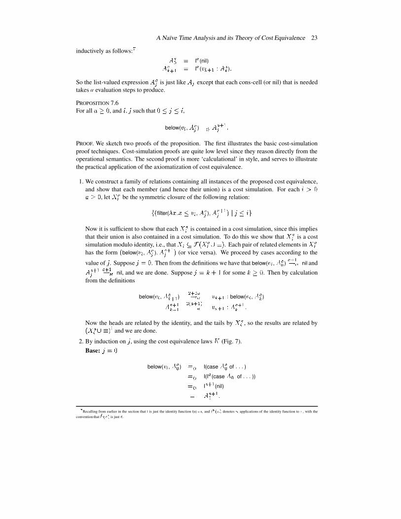
inductively as follows: � Ð��® � I�(nil)Ð��Y ± � � I�( Z Y ± � 9 Ð��Y ) 2
So the list-valued expressionÐ �Í is just like
Ð Í except that each cons-cell (or nil) that is neededtakes { evaluation steps to produce.
PROPOSITION 7.6For all {�¬~¡ , and ¯ 0 Ï such that ¡¼��Ï|�~¯ ,
below( Z . , Ð��Í ) �¼ÔÖÕ Ð � ± �Í 2PROOF. We sketch two proofs of the proposition. The first illustrates the basic cost-simulationproof techniques. Cost-simulation proofs are quite low level since they reason directly from theoperational semantics. The second proof is more ‘calculational’ in style, and serves to illustratethe practical application of the axiomatization of cost equivalence.
1. We construct a family of relations containing all instances of the proposed cost equivalence,and show that each member (and hence their union) is a cost simulation. For each ¯ë ¡{�¬~¡ , let � �. be the symmetric closure of the following relation:J � filter( Øh/ 2 /e�~Z . , Ð��Í ) 0 Ð � ± �Í : Ï|�~¯�ONow it is sufficient to show that each � �. is contained in a cost simulation, since this impliesthat their union is also contained in a cost simulation. To do this we show that � �. is a costsimulation modulo identity, i.e., that � . ß�Þe��� �. �ê�� . Each pair of related elements in � �.has the form � below( Z . , Ð �Í ) 0 Ð � ± �Í (or vice versa). We proceed by cases according to the
value of Ï . Suppose Ï[��¡ . Then from the definitions we have that below( Z . , Ð��® )� ± �P U nil andÐ � ± �Í � ± �PBU nil, and we are done. Suppose Ï|�×·�� � for some ·B¬�¡ . Then by calculation
from the definitions
below( Z . , Ð��Y ± � ) � ± � �P U Z Y ± � 9 below( Z . , Ð��Y )Ð � ± �Y ± � � � � ± ���PBU Z Y ± � 9 Ð � ± �Y 2Now the heads are related by the identity, and the tails by � �. , so the results are related by��� �. �ú�� 9 and we are done.
2. By induction on Ï , using the cost equivalence laws � (Fig. 7).Base: Ïë��¡
below( Z . , Ð �® ) � ÔÖÕ I(caseÐ �® of 2�2�2 )� ÔÖÕ I(I
�(case
Ð ® of 2�2�2 ))�¼ÔÖÕ I� ± � (nil)� Ð � ± �® 2
Recalling from earlier in the section that I is just the identity function I(x) = x, and I !�"��$# denotes % applications of the identity function to � , with theconvention that I &'"��$# is just � .

24 A Naıve Time Analysis and its Theory of Cost Equivalence
Induction: Ïë��·�� �below( Z . , Ð��Y ± � ) �¼ÔÖÕ I(case
Ð��Y ± � of …)�¼ÔÖÕ I� ± � (case Z Y ± � 9 Ð��Y of …)�¼ÔÖÕ I� ± � (if Z . �~Z Y ± � then Z Y ± � :below( Z . , Ð��Y ) else 2�2�2 )�¼ÔÖÕ I� ± � ( Z Y ± � :below( Z . , Ð��Y ))�¼ÔÖÕ I� ± � ( Z Y ± � :
Ð � ± �Y) (Hypothesis)� Ð � ± �Y ± � 2
Remark While a proof using the cost-equivalence laws and simple induction may be preferable,the proof method of constructing a cost simulation is strictly more powerful—for example, itallows the proposition be generalized to include possibly infinite non-increasing lists (althoughthis generalization is not relevant in the context of the sorting example).
Now we can return to quicksort. We consider the more general caseof ( qs(Ð��Í ) ) � . Considering
the cases when Ï[��¡ and Ï[��·�� � , and instantiating the general time equation gives� qs(Ð��® ) �� � � ��� Ð��® ���� � ��{( qs(
Ð��Y ± � ) ) � � � � ( Ð��Y ± � ) � � � �~� qs(below( Z Y ± � ,Ð��Y
)) ���� ¨©��{`�~� qs(below( Z Y ± � ,Ð��Y
)) � � 2We can simplify the right-hand side by the proposition, to give( qs(
Ð��Y ± � ) ) � �~¨©��{`�*( qs(Ð � ± �Y
) ) � 2Again the recurrence is easily solved; a simple induction is sufficient to check that� qs(
Ð��3 ) ���� ������¾C ¨ �l{4��� � �� � 2Since the
Ð 3 are justÐ ®3 , we finally have� qs(
Ð 3 ) ���� ��|��¾C ¨ � � 28 Higher-order functionsOne advantage of a simple operational approach to reasoning about programs is the relative easewith which we can handle higher-order functions. In this section we show how the time rulescan be easily extended to cope with the incorporation of the terms and evaluation rules of thelazy lambda calculus [1]. The only potentially difficult part is the extension of the theory of costequivalence. We sketch how the precongruence proof for cost simulation can be extended, withfew modifications, to handle lambda terms and their application.
8.1 The lazy lambda calculus
We consider an extension to the language with the terms and evaluation rules of the lazy lambdacalculus[1, 29]. The lazy lambda calculus, + , shares the syntax of the pure untyped lambda

A Naıve Time Analysis and its Theory of Cost Equivalence 25
calculus, but has an operational semantics which is consistent with implementations of higher-order functional languages, namely, there is no evaluation ‘under a lambda’.
The usual definitions of free and bound variables in lambda terms apply, and we do not repeatthe definitions here. The evaluation rules for application and lambda terms are given below:
lambda Øh/ 2 �©PBR�Øh/ 2 �apply
� � PBUbØE/ 2 � � J � ��K /�O`PBRQS� � � � P_R�S 2Remark Notice that we do not evaluate under a lambda even in the case of evaluation to ‘normal-form’. This is consistent with the printing mechanisms provided for higher-order functionallanguages that allow functions to be the top-level results of programs. However, in the sequel wefocus purely on the P U relation.
In the analysis of cost we choose additionally to count the number of times we invoke the applyrule in the evaluation of a term. The extension of the time rules is completely obvious:�%Øh/ 2 ���)* � ¡�%� � � � � * � � ���%� � ���j�~��� J � ��K /�O1� * 0 if � � PBUBØh/ 2 � 28.2 Applicative cost simulation
We will sketch the following:q the extension of the definition of cost simulation to applicative cost simulation;q the proof that applicative cost simulation is a precongruence.
The extension of the definition of cost simulation to handle the case where an expressionevaluates to a lambda expression follows the definition of applicative (bi)simulation [1].
DEFINITION 8.1If Ù is a binary relation on closed expressions, then Ù-, is the binary relation on lambdaexpressions such that ��Øh/ 2 � � Ù.,�Ø w 2 � � if and only if for all closed expressions � , ��Øh/ 2 � � )�óÙ�Ø w 2 � � )�
As in Definition 6.5 we define applicative cost simulation as the maximal fixed point of amonotone function: For each binary relation z on closed expressions, define the relation /e��z� by �0/��z� �� r ��@ if � fP Ubk
then �Lr fP UBk r for some k rsuch that k � Ù 9 �BÙ.,] k r 2
Now we say that a relation � is an applicative cost simulation if ���/e���Π.DEFINITION 8.2 (Applicative cost simulation)
Let 1 denote the largest applicative cost simulation, the maximum fixed point of /�� M , given by2 J ��9C���/����Π=O
26 A Naıve Time Analysis and its Theory of Cost Equivalence
It is again straightforward to show that 1 is a preorder. We prove that 1 is preserved bysubstitution into arbitrary (closed) contexts by a direct extension of the proof of that for å(Lemma 6.10 and Theorem 6.11). As before we construct a relation which contains 1 and allclosed substitution instances and show that it is a cost simulation.
THEOREM 8.3 (Precongruence II)If í��1�í�Lr for some commonly indexed families of closed expressions í� 0 í��r , then for all expressions� containing at most variables í/ � J í� K í/hO�1j� J í� r K í/hO 2The proof is sketched in Appendix A.
Again the use of the term congruence could be challenged since we do not consider openexpressions whose free variables are captured by the context. As before we can extend applicativecost simulation to open expressions � and ��r , by saying �31 �=r if ��ð41²��ðîr for all closingsubstitutions ð . It is then easy to show that, for example, Øh/ 2 ��1~Øh/ 2 ��r .9 A further exampleIn this section we present a final example. It gives a good illustration of the use (and proof) ofcost equivalence in the derivation of a time property. The reader is invited to attempt an analysiswithout the use of cost equivalence.
9.1 Maxtails
Figure 8 defines some functions including max, which computes the first element, according todictionary order, of a list of words. Words are represented as lists of characters. max employs anauxiliary binary comparison on words, dmax, which in turn employs a primitive function precedeswhich tests if one character precedes another.
Two abbreviations have been adopted to aid presentation: parentheses have been elided in theapplication of unary functions, and a function name f ( -ary) written directly denotes the obviousabstraction ØE/ ��2�2�2�2 Øh/63 2 f ��/ �N2�2�2 /43E .
In what follows we will denote words just by the concatenation of the elements (so, for example,aab represents the list a:a:b:nil). We can thus illustrate the functionality of dmax by saying thatdmax(a,aa) P a a and dmax(aa,ab) P a aa.
The object of the example is the function maxtails, which computes the dictionary maximumof the non-empty tails of a list. For example, the tails of aba are aba, ba and a, of which a is the‘maximum’. The objective is, at first sight a modest one. We wish to show that maxtails can takequadratic time (in the length of the list argument) to produce a normal form.
The quadratic time result is not obvious because of the interaction of the lazy evaluation orderand the (lazy) lexicographic ordering, which very often gives good performance. For example,maxtails is linear on the following classes of lists:q lists of strictly ‘decreasing’ elements eg. abcde…,q lists of strictly ‘increasing’ elements, eg. zyx…, andq stationary lists, eg bbb….
The proofs of these properties are left as exercises.

A Naıve Time Analysis and its Theory of Cost Equivalence 27
maxtails xs = max (tails xs)
max xs = case xs ofnil @ undefinedh:t @ foldr(dmax,h,t)
dmax(xs,ys) = case ys ofnil @ nilh:t @ case xs of
nil @ nilh’:t’ @ if h=h’ then h: dmax(t’,t)
else if (h precedes h’) then h:t else h’:t’
tails ys = case ys ofnil @ nilh:t @ (h:t): tails t
foldr(f,b,xs) = case xs ofnil @ bh:t @ f h foldr(f,b,t)
FIG. 8. Maxtails
9.1.1 OverviewThe remainder of this section builds a proof of the above quadratic time property. We breakthe proof down into a number of distinct steps, each of which illustrates some techniques forreasoning using cost equivalence.
The first step is to find a simpler representation of the problem via a cost equivalence: wederive a recursive function and recast the problem in terms of properties of this new function.The second step is to find a family of lists that will yield the quadratic time result (we just givesome informal motivation at this point). Now, as in the quicksort example, we find a crucialsimplifying cost equivalence relating to this family of lists. Given these steps the final timeanalysis is straightforward.
9.2 An equivalent problem
From the cost-equivalence laws, including the case law from Proposition 7.1, we have that
max (tails x) � ÔÖÕ I �576�8:9 (tails x) ofnil @ undefinedh:t @ foldr(dmax,h,t))� ÔÖÕ I ���576�8:9 x of
nil @ undefinedh:t @ foldr(dmax,(h:t),tails t))
2

28 A Naıve Time Analysis and its Theory of Cost Equivalence
Now we wish to proceed by analysing the expression foldr(dmax,(h:t),tails t). We derive a recursivefunction for the slightly more general expression foldr(dmax,y,tails xs). The function fot we derivewill satisfy fot(y,xs) �|Ô Õ I(foldr(dmax,y,tails xs)) 2 Initially we can satisfy this by defining
fot(y,xs) = foldr(dmax,y,tails xs).
We consider this to be an initial specification of fot, and proceed by transforming the right-handside in the manner of unfold fold transformation [12], maintaining cost equivalence:
foldr(dmax,y,tails xs)� ÔÖÕ I(case (tails xs) ofnil @ yh:t @ I � (dmax(h,foldr(dmax,y,t))))
(unfold foldr)�¼ÔÖÕ I � (case xs ofnil @ yh:t @ I � (dmax((h:t),foldr(dmax,y,tails t))))
(unfold tails, case law)�¼ÔÖÕ I � (case xs ofnil @ yh:t @ I
<(case foldr(dmax,y,tails t) of…)))
(unfold dmax)� ÔÖÕ I � (case xs ofnil @ yh:t @ I � (case I(foldr(dmax,y,tails t)) of…)))
(case law)� ÔÖÕ I � (case xs ofnil @ yh:t @ I(dmax((h:t),I(foldr(dmax,y,tails t)))))
(fold dmax)�¼ÔÖÕ I � (case xs ofnil @ yh:t @ I(dmax((h:t),fot(y,t))))
2 (fot spec.)
So we obtain a recursive definition
fot(y,xs) = I � (case xs ofnil @ yh:t @ I(dmax((h:t),fot(y,t))))
2PROPOSITION 9.1fot(y,xs) �¼ÔÖÕ I(foldr(dmax,y,tails xs))
PROOF. The above derivation constitutes a proof, although the fact that this is a proof needs somefurther justification, and depends critically on the fact that the steps are cost equivalences—see[40], but we can also prove it directly by the usual method of showing that it is a simulation. Thedetails are left as an exercise.

A Naıve Time Analysis and its Theory of Cost Equivalence 29
We are interested in computing the normal-form of maxtails � . From the above cost equivalences,we have that:� maxtails ��� ! � � � �
I � >?case � of
nil @ undefinedh:t @ foldr(dmax,(h:t),tails t)
FG � !� � � �
I
>?case � of
nil @ I undefinedh:t @ I foldr(dmax,(h:t),tails t)
FG � !� ¨©� �
case � ofnil @ I undefinedh:t @ fot((h:t),t) � ! 2
9.3 A quadratic case
Informally speaking, dmax evaluates enough of its arguments to determine which is the answer.So the amount of evaluation is bounded by the length of the answer. This suggests that to obtainworst-case inputs for maxtails, the size of the result should be ���� , where is the length ofthe input. Furthermore, to force dmax to ‘recurse’ often, the various tails of the input should be,as far as possible, element-wise equal. Inputs of the form a…ab satisfy these requirements— theresult is the input itself, and any pair of tails, eg. aaaab and aab, are element-wise equal up to butnot including the last element of the shorter.
DEFINITION 9.2For ·e¬Ì¡ , let { Y } denote the list consisting of · as followed by a single b.
We will show that this family of lists gives rise to quadratic time performance.The following family of functions will be instrumental in expressing a key cost equivalence
DEFINITION 9.3The functions
JTY O Y Ñ ® are given by the following scheme:
T ® xs � xsTY ± � xs � 576�8:9 xs of
nil @ nilh:t @ h:(T
Yt)
2For list-valued arguments, T
Y‘traverses’ its argument up to a depth · . The following properties
of the TY
follow easily:
PROPOSITION 9.4
1. T ® �`� ÔÖÕ I( � ).2. T
Y ± � ( � � : � � ) �¼ÔÖÕ I( � � :TY � � ).
3. For all expressions � such that �`P a Z � 9 2�2�2 Z"Í|9 nil, Ï|¬~¡ ,� T Y ���!�� � ��;�{]/���Ï 0 ·4 ��~�����! 2Before we state the key cost equivalence we need one technical construction:
30 A Naıve Time Analysis and its Theory of Cost Equivalence
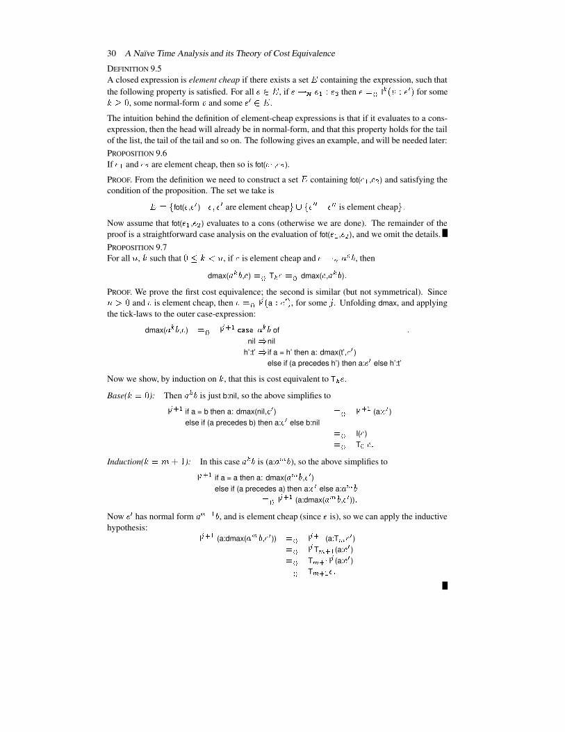
DEFINITION 9.5A closed expression is element cheap if there exists a set , containing the expression, such thatthe following property is satisfied. For all �ë�V, , if �`PbUB� � 9C� � then �`�¼ÔÖÕ I
Y �Z�9C�=r� for some·�¬Ì¡ , some normal-form Z and some ��r��Ú, .
The intuition behind the definition of element-cheap expressions is that if it evaluates to a cons-expression, then the head will already be in normal-form, and that this property holds for the tailof the list, the tail of the tail and so on. The following gives an example, and will be needed later:PROPOSITION 9.6If � � and � � are element cheap, then so is fot( � � , � � ).
PROOF. From the definition we need to construct a set , containing fot( � � , � � ) and satisfying thecondition of the proposition. The set we take is,�� J
fot( � , �=r ) : � 0 � r are element cheap O<� J � r'r : �Lr'r is element cheap O 2Now assume that fot( � � , � � ) evaluates to a cons (otherwise we are done). The remainder of theproof is a straightforward case analysis on the evaluation of fot( � � , � � ), and we omit the details.PROPOSITION 9.7For all , · such that ¡¼�~·e°j , if � is element cheap and �`P a { 3 } , then
dmax( { Y } , � ) � ÔÖÕ TY �©� ÔÖÕ dmax( � , { Y } ) 2
PROOF. We prove the first cost equivalence; the second is similar (but not symmetrical). SincesÂ�¡ and � is element cheap, then ��� ÔÖÕ IÍ � a 9]�=rT , for some Ï . Unfolding dmax, and applyingthe tick-laws to the outer case-expression:
dmax( { Y } , � ) � ÔÖÕ IÍ ± �=576�8:9_{ Y } ofnil @ nil
h’:t’ @ if a = h’ then a: dmax(t’, � r )else if (a precedes h’) then a: �=r else h’:t’
2Now we show, by induction on · , that this is cost equivalent to T
Y � .
Base( ·���¡ ): Then { Y } is just b:nil, so the above simplifies to
IÍ ± � if a = b then a: dmax(nil, �=r )else if (a precedes b) then a: �=r else b:nil
�[ÔÖÕ IÍ ± � (a: �Lr )�[ÔÖÕ I( � )�[ÔÖÕ T ®£� 2Induction( ·��>;+� � ): In this case { Y } is (a: { � } ), so the above simplifies to
IÍ ± � if a = a then a: dmax( { � } , �=r )else if (a precedes a) then a: �=r else a: { � }� Ô Õ IÍ ± � (a:dmax( { � } , �=r )) 2
Now �Lr has normal form { 3 ò �u} , and is element cheap (since � is), so we can apply the inductivehypothesis:
IÍ ± � (a:dmax( { � } , �=r )) �¼ÔÖÕ IÍ ± � (a:T � �Lr )�¼ÔÖÕ IÍ T � ± � (a: �=r )�¼ÔÖÕ T � ± � IÍ (a: �=r )� ÔÖÕ T � ± � � 2

A Naıve Time Analysis and its Theory of Cost Equivalence 31
9.4 The final analysis
We now draw the components together to show that maxtails { 3 } is ������L . First, assume sÂj¡ .From the simplifying cost equivalence in Section 9.2 we have that� maxtails { 3 }L� ! � ¨©� �
case { 3 } ofnil @ I undefinedh:t @ fot((h:t),t) � !
� ¨©� ( fot( { 3 } , { 3 ò �u} ) ) ! 2Now we take advantage of our knowledge of the extensional properties of maxtails (withoutproof)—in particular, that the normal-form of fot( { 3 } , { � } ) for any ;v°~ is { 3 } . In the generalcase where VÂ?;vÂ~¡ we have that� fot( { 3 } , { � } ) � ! � Ó£� ( dmax( { � } ,fot( { 3 } , { � ò �L} )) ) !� Ó£�>( T � fot( { 3 } , { � ò �L} ) ) ! �@ yBA ; �C 2ED 0 @ yBA ; �$C 2EF � Ó£�G;+�H( fot( { 3 } , { � ò ��} ) ) ! �@ yBA ; �C 2 I ) 2The case when VÂ?;Û��¡ is given by direct calculation from the time rules:� fot( { 3 } , } ) � !��HJ 2So we can solve this recurrence when sÂH;v¬j¡ to give� fot( { 3 } , { � } ) ��!��ô� �K � ¯% ��lÓL;×��J 2So returning to the main problem,� maxtails { 3 }"� ! � ¨©�*( fot( { 3 } , { 3 ò �L} ) ) !� ¨©� �M 3 ò �� ¯% ��lÓ]��» � ���J� �� ����� � ��l¨H|� F42Final remark Some of the intermediate steps are more general than necessary to obtain thisresult. In particular the technicalities Definition 9.5–Proposition 9.7 regarding element-cheapexpressions and the properties of dmax could be eliminated by a more direct proof in the finalanalysis above, but they help make the result robust with respect to, for example, the order inwhich the tails are ‘folded’ together. For example it is an easy exercise to show that replacingfoldr by a ‘fold from the left’ does not essentially change this quadratic-time case.
10 Call-by-need and compositionalityThe calculus is betrayed by its simple operational origins because it describes a call-by-nameevaluation mechanism, when most actual implementations of lazy evaluation use call-by-need.For example, consider the definition
average(xs) = divide(sum(xs),length(xs))
where divide is a primitive function, and sum and length are the obvious functions on lists. Inreasoning about the evaluation of an instance, average( � ), our method will overestimate the
32 A Naıve Time Analysis and its Theory of Cost Equivalence
evaluation time, because of the duplication of expression � on substitution into the body ofaverage. Assuming � has a normal-form which is a non-empty list of integers, to compute thenecessary calls to sum and length each cons in the result of � must be computed, but this workwill be performed independently by sum and length using their own copies of � , whereas undercall-by-need this evaluation (and hence its cost) will be shared.
One solution is to work with an operational model that takes into account the sharing ofexpressions and evaluations [5]. Unfortunately this may overly complicate the calculus, andis likely to be impractical—although there are some promising (less general) approaches tomodelling sharing and storage, [3, 25], which may be prove usable.
Another solution is to move towards the compositional approaches mentioned in the introduc-tion. A suitable interface between the compositional approach in [37] (which differs from thatof [42] in its use of genuine strictness rather than absence information) from and the operationalapproach of this paper is via Burn’s notion of an evaluator [10]. An evaluator is an operationalconcept which provides a link from information provided by (list-based extensions of) strictnessanalysis, to the operational semantics. In particular, strictness analysis [11] will tell us that whenan application of average is being evaluated, it is safe to evaluate the argument to normal-form(since this evaluation will occur anyway). In terms of our calculus, by taking into account (inadvance) the amount of evaluation that must be performed on the argument, we obtain a morecompositional analysis, and a better approximation to call-by-need, using:� average( � ) � � �+�%��� ! ��� average( Z ) � � 0 where �`P a Z .
In this section we describe a new formalization of evaluators appropriate for providing asmooth interface between compositional and non-compositional (call-by-need and call-by-name)approaches to time analysis. The development is for the first-order language, although it can beused within higher-order programs.
10.1 Demands
Burn’s formalization of evaluators is couched in terms of reduction strategies in a typed lambdacalculus with constants. An evaluator is defined, relative to a particular (Scott) closed set ofdenotations, as any reduction strategy which fails to terminate exactly when the denotation of theterm is in the set. For example, the leftmost outermost reduction strategy fails to terminate if andonly if the denotation of the term is in the Scott-closed set
JLN O .However, the definition of an evaluator is not constructive. Given a Scott-closed set, Burn does
not provide an operational definition of an evaluator for that set.In the approach we have taken to the operational semantics of the language, issues of reduction
strategy are internalized by the evaluation relations. In order to use the evaluator concept inreasoning about evaluation cost we need a constructive definition of evaluators. We will define afamily of evaluators, and show how the relations P a and PBU can be viewed as instances. Thestarting point of this definition is a language of demands.
We interpret a demand as a specification of a degree of evaluation, and define a demand-parameterized evaluation relation which realises these demands. Bjerner and Holmstrom [8]use a particularly simple language of demands in the context of compositional time analysis.Their interpretation of a demand only makes sense relative to a particular expression: a demandon an expression is a representation of an approximation to its denotation. Their language ofdemands is too ‘precise’ for our purposes. The language of demands which we use will becloser to that of, for example, Lindstrom’s lattice of demands [23] or Dybjer’s formal opens

A Naıve Time Analysis and its Theory of Cost Equivalence 33
[14], and our interpretation of demand, as in [14], will be closely related to strictness. Theoperational interpretation of demand as an evaluator is, in turn, reminiscent of Bjerner’s definitionof computing an expression to one of its proper evaluation degrees [7].
DEFINITION 10.1The language of demands, O��-P is given byPÀ�>Q :BRÚ: P � 9ù9 P � :�R ��P � 979 P � :�S / 2 �P� : / 2The demand Q is the zero-demand which is satisfied by any expression. The demand
Ris satisfied
by any expression which evaluates to a constant, including nil (we could easily extend the demandsto include demands for each individual constant). The cons-demand P � 979EP � is satisfied by anyexpression which evaluates to a cons, and whose head and tail satisfy P � and P � respectively.We have a restricted form of disjunctive demand for either a constant or a cons, and finally weadd a recursive demand useful for specifying demands over lists.
This informal reading of a demand can easily be formalized, and the set of expressions whichsatisfy a demand can be shown to be open with respect to the usual operational preorder (c.f.[14]).We do not pursue this formalization here, but just focus on the operational interpretation ofdemands as evaluators.DEFINITION 10.2For each closed demand O we define an associated evaluator ��@�T . The family of evaluators isdefined by inductively as the least relations between closed expressions that satisfy the followingrules: �©��@-U�� �`P U I�`��@WV I�©PBUb� � 9C� � � � ��@ T # � r � � � ��@ T # � r �����@XT #:Y Y T p � r � 9C� r ��`��@WV[� r�`��@XV ± T # Y Y T p � r �`��@ T # Y Y T p � r�`��@WV ± T # Y Y T p � r����@ T:Z:[�\^] � T �`_ \Ba � r
.�`��@ [�\^] � T � � rNote that the evaluators are defined using the basic reduction engine, P U . It is not difficult
to show that evaluators are deterministic (i.e., each ��@�T is a partial function) and that proofs ofevaluation judgements are unique. As for PbR , we write � f��@ T �=r when ����@ T �Lr and its proofuses «©¬~¡ instances of rule Fun.
Now we can show that the previous evaluation relations can be viewed as instancesof evaluators:
PROPOSITION 10.3
1. � f��@�V ± U Y Y U �=r���@ � fP_UB�=r2. � f��@ [�\L] � V ± \ Y Y \ � � r ��@ � fPBab� r
PROOF. 1. The first part is simple. ( @ ) follows from the definition of evaluators, ( � ) byconsidering the two cases for ��r .
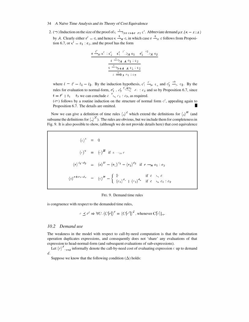
34 A Naıve Time Analysis and its Theory of Cost Equivalence
2. ( @ ) Induction on the size of the proof of � f��@ [�\^] � V ± \ Y Y \ � �=r . Abbreviate demandS / 2 � R ��/N979 /h
byÐ
. Clearly either �=r�� I, and hence � fP U I
, in which case � fPBa Ifollows from Proposi-
tion 6.7, or �=rE��� � 9C� � , and the proof has the form� f�bP_UB� r � 9C� r � � r � f ���@dcê� � � r � f ���@ec¿� �� f��@ c Y Y c � � 9H� �� f��@ V ± c Y Y c � � 9C� �� f��@dcê� � 9C� �where «ë� «)r6�Ì« � �Ì« � . By the induction hypothesis, ��r � f �P a � � and �=r � f �P a � � . By the
rules for evaluation to normal-form, ��r � 96�Lr� f # ± f pPBa � � 96� � and so by Proposition 6.7, since«Ê��«)r]�ê« � ��« � we can conclude � fPBaB� � 9C� � , as required.( � ) follows by a routine induction on the structure of normal form ��r , appealing again toProposition 6.7. The details are omitted.
Now we can give a definition of time rules � � T which extend the definitions for � � � (andsubsume the definitions for � ��! ). The rules are obvious, but we include them for completeness inFig. 9. It is also possible to show, (although we do not provide details here) that cost equivalence
����� U � ¡���� V � ������� if �`P U I����� T # Y Y T p � ����� � ���%� � � T # �~��� � � T p if �`PBUB� � 9C� ������ V ± T #fY Y T p � �������j��� ¡ if ��P U I�%� � � T # �~��� � � T p if ��PBUb� � 9H� �FIG. 9. Demand time rules
is congruence with respect to the demanded time rules,��åÌ� r @¢ãî$ 2 ��$�&'� ( � T �×��$�&'� r ( � T 0 whenever $�&'� (�øBg 210.2 Demand use
The weakness in the model with respect to call-by-need computation is that the substitutionoperation duplicates expressions, and consequently does not ‘share’ any evaluations of thatexpression to head-normal-form (and subsequent evaluations of sub-expressions).
Let ����� T�h7i$i$j informally denote the call-by-need cost of evaluating expression � up to demandO .Suppose we know that the following condition ( � ) holds:
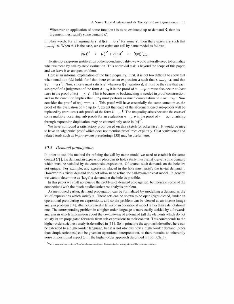
A Naıve Time Analysis and its Theory of Cost Equivalence 35
Whenever an application of some function f is to be evaluated up to demand O , then itsargument must satisfy some demand OXr .
In other words, for all arguments � , if f( � ) ��@ T �=r for some �=r , then there exists a S such that����@ T b S . When this is the case, we can refine our call by name model as follows.� f( � ) � T ¬ ����� T b ��� f( S ) � T ¬ � f( S ) � Th7i$i$j 2To attempt a rigorous justification of the second inequality, we would naturally need to formalize
what we mean by call-by-need evaluation. This nontrivial task is beyond the scope of this paper,and we leave it as an open problem.
Here is an informal explanation of the first inequality. First, it is not too difficult to show thatwhen condition ( � ) holds for f that there exists an expression S such that ����@-T b S , and thatf( S ) ��@XT��Lr 2 k Now, since � must satisfy OXr whenever f ��� satisfies O , it must be the case that eachsub-proof of a judgement of the form {�P U } in the proof of ����@WT b S must also occur at leastonce in the proof of f( � ) ��@WT��Lr . This is because no backtracking is needed in proof construction,and so the condition implies that ��@.T must perform as much computation on � as ��@.T b . Nowconsider the proof of f( S ) ��@WTe� r . This proof will have essentially the same structure as theproof of the evaluation of f( � ) up to O , except that each of the aforementioned sub-proofs will bereplaced by (zero-cost) sub-proofs of the form }£PbUb} . The inequality arises because the costs ofsome multiply-occurring sub-proofs for an evaluation {�PbUê} in the proof of ����@ T b S , arisingthrough expression duplication, may be counted only once in �%��� T b .
We have not found a satisfactory proof based on this sketch (or otherwise). It would be niceto have an ‘algebraic’ proof which does not mention proof-trees explicitly. Cost equivalence andrelated tools such as improvement preorderings [38] may be useful here.
10.3 Demand propagation
In order to use this method for refining the call-by-name model we need to establish for somecontext $�& ( , the demand an expression placed in its hole satisfy must satisfy, given some demandwhich must be satisfied by the composite expression. Of course, such demands on the hole arenot unique. For example, any expression placed in the hole must satisfy the trivial demand Q .However this trivial demand does not allow us to refine the call-by-name cost model. In generalwe want to determine as ‘large’ a demand on the hole as possible.
In this paper we shall not pursue the problem of demand propagation, but mention some of theconnections with the much-studied strictness analysis problem.
As mentioned earlier, demand propagation can be formalized by modelling a demand as theset of expressions which satisfy it. These sets can be shown to be open (right-closed) under anoperational preordering on expressions, and so the problem can be viewed as an inverse-imageanalysis problem [14], albeit expressed in terms of an operational model rather than a denotationalone. The corresponding problem in a higher-order language is more easily tackled by a forwardsanalysis in which information about the complement of a demand (all the elements which do notsatisfy it) are propagated forwards from sub-expressions to their context. This corresponds to thehigher-order strictness analysis described in [11]. So in principle the approach described here canbe extended to a higher-order language, but it is not obvious how a higher-order demand (otherthan simple strictness) can be given an operational interpretation, so there remains an inherentlynon-compositional aspect (c.f.. the higher-order approach described in [36], Ch. 5).l
This is a constructive version of Burn’s evaluation transformer theorem—further investigations will be presented elsewhere.

36 A Naıve Time Analysis and its Theory of Cost Equivalence
10.4 Comparison with earlier compositional approaches
Here we place the approach outlined in this section in comparison with the compositional methodsfor time analysis overviewed in Section 2. The use of demands to refine call-by-name evaluationtime to give a better approximation to call-by-need is consistent with the use of strictness infor-mation in necessary-time analysis [35]. The key difference is that strictness information is usedby necessary-time analysis to give a lower bound to call-by-need computation cost, whereas it isused here to give an upper-bound (which in turn is bounded above by call-by-name cost). In bothcases the quality of demand information determines the tightness of the bound. We would arguethat the method here is more useful.
The time analysis described by Wadler [42] (which is the first order instance of sufficient-timeanalysis in [35]) also gives an upper-bound to call-by-need time, but in a rather different manner:it uses information about ‘absence’ (constancy) which describes what parts of an expression willnot be evaluated. Unfortunately in this case although the quality of this upper bound is determinedby the quality of this ‘absence’ information, m this upper-bound may not be well defined even whenthe program is.
The approach described by Bjerner and Holmstrom [8] is a fully compositional method forreasoningabout first-order functional programs with lazy lists. This approach is harder to comparebecause the ‘demand’ information is exact; the call-by-need time analysis is therefore exact aswell (although, as here, the treatment of call-by-need is not formalized). This precision, as theauthors note, is also a serious drawback in reasoning about programs, since as a first step one mustdecide what ‘demand’ to make on the output. Since the language of demands is so precise, inorder to reason about computation of a program to normal form one must begin with the demandthat exactly describes that normal form—in other words (a representation of) the normal formitself. It is not immediately obvious how to introduce ‘approximate’ demands in this approachwithout running into the definedness problems of Wadler’s method.
To summarize, the approach sketched in this section has the following advantages:q it provides a safe (well-defined) time bound lying between call-by-need and call-by-namecosts;q it allows flexibility in the use of demand information so it can be targeted to where either
1. more compositionality is needed to decompose the time analysis of a large program, or
2. where (it is suspected that) the call-by-name model is too crude.
Although our method and exposition were inspired by formulating a constructive (operational)version of Burn’s evaluators, in retrospect the approach is much closer to Bjerner’s original workon time analysis of programs of type theory, because of it’s operational basis. The connec-tion to evaluators does not occur in Bjerner’s work because of the absence of non-terminatingcomputations in that language.
11 Related workHere we review work related to the theory of cost simulation.n
Quality should not be confused with safety—we assume that the information is always safe in the sense that whenever it predicts a property of a program, theproperty does indeed hold.
A Naıve Time Analysis and its Theory of Cost Equivalence 37
11.1 Other non-standard theories of equivalence
Talcott [41] introduced a broad semantic theory of side-effect-free Lisp-like languages, notablefor its treatment of both extensional and intensional aspects of computation. In particular a classof preorderings called comparison relations were introduced for a side-effect-free Lisp derivative.The method of their definition is similar to the definition of operational approximation as a Park-style simulation, although the cost aspects are not built into this definition directly as they arehere. Nonetheless, the class of comparison relations could be said to contain relations analogousto the cost-equivalence relation considered here (this is just the observation that cost simulationcan be viewed as a refinement of a pure simulation not involving time properties), and indeed itis suggested (as a topic for further work) that certain comparison relations could be developedto provide soundness and improvement proofs for program transformation laws. However,only the ‘maximal’ comparison relations (essentially, the more usual operational approximationand equivalence relations) and their application are considered in detail. Following on fromother aspects of this work, Mason [24] sketches the definition a family of equivalence relationsinvolving a variety of operation execution counts. However, as this is for a pure language withneither higher-order functions nor lazy data structures, the relations have a relatively uninterestingstructure.
Moggi’s categorical semantics of computation [28] is intended to be suitable for capturingbroader descriptions of computation than just input–output behaviour. Gurr [16] has studiedextensions of denotational semantics to take account of resource use, and has shown how Moggi’sapproach can be used to model computation in such a way that program equivalence also capturesequivalence of resource requirements. Gurr extends Moggi’s Ø�ý -calculus (a formal system forreasoning about equivalence) with sequents for reasoning about the resource properties directly(although the ability to do this depends on certain ‘representability’ issues, not least of all that theresource itself should correspond to a type in the metalanguage). The resulting calculus is dubbed‘ Ø ý$o � ’. We can compare this to the approach taken here, where cost equivalence (a ‘resource’equivalence) is used in conjunction with a set of time rules which are used to reason about thecost property directly. There are further analogies in the details of Gurr’s approach: he definesrules for sequents of the form p � ,Bqsrut �%� 0 Z 0 «u�©9^vwhich says that expression � has value Z (of type v ) and consumes resource « . He goes on toshow that these rules are redundant since their information can be expressed in the Ø ý calculus(with the addition of some specific axioms). In particular the above entailment would implyp � ,Bq<wyx7z /���«|{~}�Z�9^vwhere « is the canonical term (of unit type) which consumes time ‘t’. Notice the similarity withour axiomatization of cost equivalence, which uses the identity function in much the same manneras the computational let is used in the Øîý calculus.
An important difference is that in our approach these concepts are derived from (and hencecorrect with respect to) the operational model, so we may argue, at least, that an operational ap-proach provides a more appropriate starting point for a semantic study of efficiency—although thedeeper connections between these approaches deserves some further study. � ® Another importantdifference is that we consider a lazy recursive data structure. One possible method for dealingwith this in the context of Moggi’s framework would be to combine it with Pitts’ co-induction# & Interestingly, Gurr gives an operational semantics (call-by-value) to terms of the � qsrut calculus, but leaves the property corresponding to our Theorem 7.5as a conjecture.

38 A Naıve Time Analysis and its Theory of Cost Equivalence
principal for recursively defined domains [32]. Other aspects of Gurr’s work are concerned withgiving a semantic framework for some aspects of (asymptotic) complexity, which is outside thescope of this work.
Another, perhaps more abstract category-theoretic approach to intensional semantics is pre-sented by Brookes and Geva [9]. This work places a heavy emphasis on the relationship betweenthe intensional semantics and its underlying extensional one. The key structure is the use of aco-monad, in contrast to Gurr’s use of Moggi’s monadic style, and it’s suitability for formulatingthe kind of intensional semantics described here is perhaps less obvious.
11.2 Program improvement and generalizations
The theory of cost simulation is significant in its own right since there are many potentiallyinteresting relations (preorders and equivalences) involving time, that can be investigated in asimilar manner. For example, consider a program refinement relation, � , which is the largestrelation such that whenever � � �~� �� � fPBU k @ � � f bPBU k r 0 for some k 0 k r such that «Ê¬�«)r
and � k � 9 k rT .Using the same approach to that of cost simulation, it can be shown that � is a (pre)congruence, �u�and consequently that for all contexts $ ,���~� r ��@¥��$�&'� ( �*e¬��%$�&'�=r ( �* 0which can be restated as ‘ ��r is at least as efficient as � in any context’. Using the same prooftechnique as illustrated in Section 7, we have a systematic means of verifying refinement laws,such as
append(append( � � , � � ), �L< ) � append( � � ,append( � � , �L< )) 2The notion of refinement is a possible semantic criterion (albeit a somewhat exacting one) for theintensional correctness of ‘context-free’ program transformations.
The main foundation for such theories of improvement and equivalence is the definition of anappropriate simulation relation, together with a proof that it satisfies the substitutivity property. Sofor each variation in the language (such as the addition of new operators) and each new definitionof what improvement means, we require these constructions. This is somewhat tedious, soin a separate study[38] the problem of finding a more general formulation of the theory ofimprovement relations is addressed. For a general class of lazy languages, it is shown how apreorder on computational properties (an ‘improvement’ ordering) induces a simulation-stylepreordering on expressions (the definitions of cost simulation and program refinement are simpleinstances). Borrowing some syntactic conventions and semantic techniques from [18], someimprovementextensionality conditions on the operators of the language are given which guaranteethat the improvement ordering is a precongruence. The conditions appear relatively easy to check.Furthermore, the higher-order language given here is studied as a special case. In this context acomputational property is considered to be a function from the proof of an evaluation judgement(the computation) to a preordered set (the set of properties, ordered by ‘improvement’). Themain result of this generalization is that the simulation preorder induced by any computationalproperty is guaranteed to be a congruence whenever the property satisfies a simple monotonicity#�#
Note that if we consider a strict refinement relation where we replace � by µ in the definition of � , then it will not be a contextual congruence.
A Naıve Time Analysis and its Theory of Cost Equivalence 39
requirement with respect to the rules of the operational semantics. This result can be generalizedto Howe’s class of structured computation systems [19].
12 ConclusionsThis paper has presented a direct approach to reasoning about time cost under lazy evaluation.The calculus takes the form of time rules extracted from a suitably simple operational semantics,together with some equivalence laws which are substitutive with respect to these rules.
The aim of this calculus is to reveal enough of the ‘algorithmic structure’ of operationallyopaque lazy functional programs to permit the use of the more traditional techniques developed inthe context of the analysis of imperative programs [2], and initial experiments with this calculussuggest that it is of both practical and pedagogical use.
A desire for substitutive equivalences for the time rules led to a theory of cost equivalence,via a non-standard notion of operational approximation called cost simulation. Cost equivalenceprovides useful extensions to the time rules (although, as we showed, from a technical point ofview it subsumes them). It is also interesting in it’s own right, since it suggests an operationallybased route to the study of intensional semantics. Initial investigations of this area are reportedin [38].
Finally, we proposed an interface of this calculus with a more compositional method whichalso improves the accuracy of the analysis with respect to call-by-need evaluation, but is ableto retain the simplicity of the naıve approach where appropriate. The compositionality is basedon an operational interpretation of evaluators to re-order computation on the basis of strictness-like properties. This model can also be used to provide a more constructive formulation ofthe evaluation transformer theorem [10], which formally connects information from strictnessanalysis with its associated optimisations. Further work is needed to strengthen the relationshipbetween cost equivalence and the compositional approach. The idea of a context-dependentbisimulation between processes, as studied by Larsen (originating with [21]), seems appropriatehere since it suggests the introduction of context ( � demand)-dependent cost simulation.
AcknowledgementsThis work has been partially funded by ESPRIT II BRA 6809 (Semantique), The Danish Nat-ural Sciences Research Council (DART project), The Department of Computer Science at theUniversity of Copenhagen (DIKU), and ESPRIT III BRA 9102 (Coordination).
Thanks for various contributions to Chris Hankin, Sebastian Hunt, Bent Thomsen (while theauthor was at Imperial College), and to various members of the Semantique project at that timefor numerous suggestions and constructive criticisms; in particular to John Hughes for suggestingthat time analysis might be completely expressed in terms of cost equivalences. More recently,thanks to the TOPPS group at DIKU and to Torben Mogensen and Kristian Nielsen in particular.Special thanks to Richard Bird, who originally suggested to me that a naıve approach couldactually be useful for reasoning about call-by-name evaluation, and most recently suggested anumber of improvements that have been incorporated into this version, including the maxtailsexample, offered by way of a ‘challenge problem’.
References[1] S. Abramsky. The lazy lambda calculus. In Research Topics in Functional Programming, D. Turner, ed., pp. 65–116.

40 A Naıve Time Analysis and its Theory of Cost Equivalence
Addison Wesley, 1990.[2] A. V. Aho, J. E. Hopcroft and J. D. Ullman. The Design and Analysis of Computer Algorithms. The Addison-Wesley
Series in Computer Science and Information Processing. Addison-Wesley, London, 1974.[3] Z. M. Ariola and Arvind. A syntactic approach to program transformation. In Proceedings of the symposium
on Partial Evaluation and Semantics-Based Program Manipulation, pp. 116–129. ACM press, SIGPLAN notices,26(9), September 1991.
[4] H. P. Barendregt. The Lambda Calculus, vol. 103 of Studies in Logic and the Foundations of Mathematics. ElsevierScience Publishers B.V., 2nd edition, 1984.
[5] H. P. Barendregt, M. C. J. D. van Eekelen, J. R. W. Glauert, J. R. Kennaway, M. J. Plasmeijer and M. R. Sleep. Termgraph rewriting. In PARLE ’87 volume II, number 259 in LNCS, pp. 191–231. Springer Verlag, 1987.
[6] R. Bird and P. Wadler. Introduction to Functional Programming. Prentice Hall, 1988.[7] B. Bjerner. Time Complexity of Programs in Type Theory. PhD thesis, Chalmers University of Technology, 1989.[8] B. Bjerner and S. Holmstrom. A compositional approach to time analysis of first order lazy functional programs.
In Functional Programming Languages and Computer Architecture, Conference Proceedings, pp. 157–165. ACMpress, 1989.
[9] S. Brookes and S. Geva. Computational comonads and intensional semantics. In Categories in Computer Science,M. P. Fourman, P. T. Johnstone, and A. M. Pitts, eds, London Mathematical Society Lecture Notes, pp. 1–44.Cambridge University Press, 1992.
[10] G. L. Burn. The evaluation transformer model of reduction and its correctness. In TAPSOFT ’91. Number 494 inLNCS, pp. 458–482. Springer-Verlag, 1991.
[11] G. L. Burn, C. L. Hankin and S. Abramsky. The theory and practice of strictness analysis for higher order functions.Science of Computer Programming, 7, 249–278, 1986.
[12] R. Burstall and J. Darlington. A transformation system for developing recursive programs. JACM, 24, 44–67, 1977.[13] P. Cousot and R. Cousot. Constructive versions of Tarski’s fixed point theorems. Pacific Journal of Mathematics,
82, 43–57, 1979.[14] P. Dybjer. Inverse image analysis generalises strictness analysis. Information and Computation, 90, 194–216, 1991.[15] R. L. Graham, D. E. Knuth, and O. Patashnik. Concrete Mathematics. Addison-Wesley, 1989.[16] D. Gurr. Semantic Frameworks for Complexity. PhD thesis, Department of Computer Science, Edinburgh, 1991.
(Available as reports CST-72-91 and ECS-LFCS-91-130).[17] T. Hickey and J. Cohen. Automating program analysis. JACM, 35, 185–220, 1988.[18] D. J. Howe. Equality in lazy computation systems. In Fourth annual symposium on Logic In Computer Science, pp.
198–203. IEEE, 1989.[19] D. J. Howe. On computational open-endedness in Martin-Lof’s type theory. In Sixth annual symposium on Logic In
Computer Science, pp. 162–172, 1991.[20] D. E. Knuth. Volume 1: Fundamental Algorithms. The Art of Computer Programming. Addison-Wesley, 1968.[21] K. G. Larsen. Context-Dependent Bisimulation Between Processes. PhD thesis, Department of Computing, Univer-
sity of Edinburgh, 1986.[22] D. LeMetayer. An automatic complexity evaluator. ACM ToPLaS, 10(2):248–266, April 1988.[23] G. Lindstrom. Static evaluation of functional programs. In ACM SIGPLAN Symposium on Compiler Construction,
pp. 196–206, 1986.[24] I. Mason. The Semantics of Destructive Lisp. Number 5 in CSLI Lecture Notes. CSLI, 1986.[25] I. Mason and C. Talcott. Equivalence in functional languages with effects. Journal of Functional Programming, 1,
287–327, 1991.[26] R. Milner. Calculi for synchrony and asynchrony. Theoretical Computer Science, 25, 267–310, 1983.[27] R. Milner and M. Tofte. Co-induction in relational semantics. Theoretical Computer Science, 87, 209–220, 1991.[28] E. Moggi. Computational lambda-calculus and monads. Technical Report ECS-LFCS-88-63, Department of
Computer Science, University of Edinburgh, 1988. (Short version in Fourth LICS Conf. IEEE 1989.)[29] C.-H. Luke Ong. The Lazy Lambda Calculus: An Investigation into the Foundations of Functional Programming.
PhD thesis, Imperial College, University of London, 1988.[30] D. Park. Concurrency and automata on infinite sequences. In 5th GI Conference on Theoretical Computer Science.
LNCS 104, Springer Verlag, 1980.[31] S. L. Peyton Jones. The Implementation of Functional Programming Languages. Prentice-Hall International Series
in Computer Science. Prentice-Hall International (UK), London, 1987.
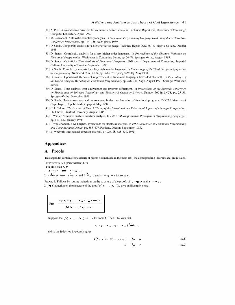
A Naıve Time Analysis and its Theory of Cost Equivalence 41
[32] A. Pitts. A co-induction principal for recursively defined domains. Technical Report 252, University of CambridgeComputer Laboratory, April 1992.
[33] M. Rosendahl. Automatic complexity analysis. In Functional Programming Languages and Computer Architecture,Conference Proceedings, pp. 144–156. ACM press, 1989.
[34] D. Sands. Complexity analysis for a higher order language. Technical Report DOC 88/14, Imperial College, October1988.
[35] D. Sands. Complexity analysis for a lazy higher-order language. In Proceedings of the Glasgow Workshop onFunctional Programming, Workshops in Computing Series, pp. 56–79. Springer Verlag, August 1989.
[36] D. Sands. Calculi for Time Analysis of Functional Programs. PhD thesis, Department of Computing, ImperialCollege, University of London, September 1990.
[37] D. Sands. Complexity analysis for a lazy higher-order language. In Proceedings of the Third European Symposiumon Programming. Number 432 in LNCS, pp. 361–376. Springer-Verlag, May 1990.
[38] D. Sands. Operational theories of improvement in functional languages (extended abstract). In Proceedings ofthe Fourth Glasgow Workshop on Functional Programming, pp. 298–311, Skye, August 1991. Springer WorkshopSeries.
[39] D. Sands. Time analysis, cost equivalence and program refinement. In Proceedings of the Eleventh Conferenceon Foundations of Software Technology and Theoretical Computer Science. Number 560 in LNCS, pp. 25–39.Springer-Verlag, December 1991.
[40] D. Sands. Total correctness and improvement in the transformation of functional programs. DIKU, University ofCopenhagen, Unpublished (53 pages), May 1994.
[41] C. L. Talcott. The Essence of Rum, A Theory of the Intensional and Extensional Aspects of Lisp-type Computation.PhD thesis, Stanford University, August 1985.
[42] P. Wadler. Strictness analysis aids time analysis. In 15th ACM Symposium on Principals of Programming Languages,pp. 119–132, January 1988.
[43] P. Wadler and R. J. M. Hughes. Projections for strictness analysis. In 1987 Conference on Functional Programmingand Computer Architecture, pp. 385–407, Portland, Oregon, September 1987.
[44] B. Wegbreit. Mechanical program analysis. CACM, 18, 528–539, 1975.
Appendices
A ProofsThis appendix contains some details of proofs not included in the main text; the corresponding theorems etc. are restated.
PROPOSITION A.1 (PROPOSITION 6.7)For all closed � , �u�
1. �=� aW����� ��� U � .
2. ���� ae� �0� � � #� UW� and � � p� ad� and � �� �`�<�X� for some � .
PROOF. 1. Follows by routine inductions on the structure of the proofs of ��� a � and ��� U.� .2. ( � ) Induction on the structure of the proof of ��� aW� . We give an illustrative case:
Fun���`��� É:�:�CÉ����u�$��� � % 5 ��� % 5�� � ae�� �� � É7�u�$���u� � % 5�¡ � a �
Suppose that� �¢�`� É����$�u��� � % 5 ¡ �� ad� for some � . Then it follows that�u����� É£�$�u� � % 5 ���Cɤ�u���`� % 5 � �s¥ É� a � �
and so the induction hypothesis gives ���¢�7� É£�u�$� � % 5 �:�Cɦ�����`� % 5 � � #� U � (A.1)� � p� a � (A.2)
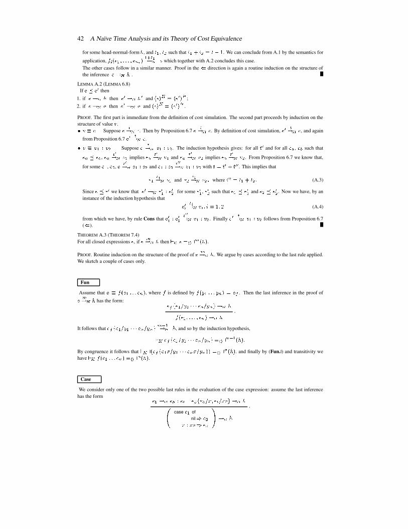
42 A Naıve Time Analysis and its Theory of Cost Equivalence
for some head-normal-form � , and � É , �`� such that � É�� �`�<�W�¨§ª© . We can conclude from A.1 by the semantics for
application,� �¢� � É����$�u��� � % 5$¡ ÉÈ � #� a � which together with A.2 concludes this case.
The other cases follow in a similar manner. Proof in the � direction is again a routine induction on the structure ofthe inference ��� U.� .
LEMMA A.2 (LEMMA 6.8)If �¬«e� � then
1. if ��� U � then �u�^� U � � and `��® é ��~�u�y® é ;2. if ��� a � then � � � a � and `��® è �¯ � � ® è .
PROOF. The first part is immediate from the definition of cost simulation. The second part proceeds by induction on thestructure of value � .° ��± � Suppose � �� a � . Then by Proposition 6.7 � �� U�� . By definition of cost simulation, �f� �� U�� , and again
from Proposition 6.7 �f� �� a�� .° ��±²� É�³ � � Suppose � �� a3� É<³ � � . The induction hypothesis gives: for all � � and for all �u´ , ��µ such that� ´ «¶��µ , � ´ � b� a � É implies �uµX� b� a � É and � ´ � b� a � � implies �uµX� b� a � � . From Proposition 6.7 we know that,
for some � É , �$� , �d� b� U � É0³ �$� and � É·³ �$��� b b� a � É·³ � � with �¸�W� � � � � � . This implies that� É � #� a � É and �$� � p� a � � � where � � � �W� É�� �`� � (A.3)
Since �·«X� � we know that � � � U � �É ³ � �� for some � �É , � �� such that � É «.� �É and �'�¹«.� �� . Now we have, by aninstance of the induction hypothesis that � �� � 5� a � � �`º �.© �» (A.4)
from which we have, by rule Cons that �u�É ³ ���� � b b� a � É·³ � � . Finally �u� �� a � É·³ � � follows from Proposition 6.7( � ).
THEOREM A.3 (THEOREM 7.4)For all closed expressions � , if �½¼� U � then ¾:¿���� ÔÖÕ I ¼ � � ¡ .PROOF. Routine induction on the structure of the proof of � ¼� U�� . We argue by cases according to the last rule applied.We sketch a couple of cases only.
Fun
Assume that � ± � �`� É£�$��� � % ¡ , where�
is defined by� �~À É£���u� À % ¡ ����Á . Then the last inference in the proof of� ¼� UX� has the form: ��ÁB�7� É7� À É£Â$Âu � % � À % � � U��
.� �`� É��u���$��� � % ¡ � U��It follows that �uÁB�7� Éf� À ÉÃÂ$Â� � % � À % � ¼ ¥ É� UÄ� , and so by the induction hypothesis,¾ ¿ �uÁB�7� É�� À É£Â�Â$ � % � À % � � ÔÖÕ I % ¥ É � � ¡ �By congruence it follows that ¾�¿ I �`� Á �7� É�Ũ� À É�ÂuÂ$ � % Ũ� À % � ¡ � Ô Õ I % � � ¡ � and finally by (Fun.I) and transitivity wehave ¾ ¿ � �`� ÉÆ���$� � % ¡ � Ô Õ I % � � ¡ .
Case
We consider only one of the two possible last rules in the evaluation of the case expression: assume the last inferencehas the form � É � U ��Ç ³ � � �'È7�7��Ç �:�¨� � � �:�^É � � U��
.Êcase � É of
nil � �'���³:�^É � �'È¶Ë � U �

A Naıve Time Analysis and its Theory of Cost Equivalence 43
It follows that � É ¼ #� U ��Ç ³ � � and �$È�����Ç �:�¨� � � �:�^É �̼ p� U � for some Í É , ÍÌ� satisfying Í É|� ÍÎ���²Í . Theinduction hypothesis then gives¾ ¿ � É � ÔÖÕ I ¼ # �`��Ç ³ � � ¡� ¾:¿ Ê
case � É ofnil � �$���³f�^É � �$È¶Ë � ÔÖÕ Ê case I ¼ # � �uÇ ³ � � ¡ of
nil � �$���³7�^É � �$ȯË� ¾ ¿ Êcase � É of
nil � �$���³f�^É � �$È¶Ë � ÔÖÕ I ¼ # Ê case � Ç ³ � � ofnil � �'���³:�^É � �'ÈÏË� ¾ ¿ Ê
case � É ofnil � �$���³f�^É � �$È Ë � ÔÖÕ I ¼ # �`�$È7�7�uÇ �:�¨� � � ���^É � ¡ �
The induction hypothesis applied to the second sub-proof gives¾ ¿ �$È��7�uÇ �:�¨� � � ���^É � � Ô Õ I ¼ p � � ¡and so by congruence (substituting the right-hand side for the left in the previous equation) we conclude that¾ ¿ Ê
case � É ofnil � �'���³7�^É � �$È Ë � ÔÖÕ I ¼ # � I ¼ p � � ¡�¡ �
and the desired result follows from the fact that I ¼ # � I ¼ p � � ¡¢¡ ± I ¼ � � ¡ .THEOREM A.4 (THEOREM 8.3)If Ð�|Ñ�Ð�u� for some commonly indexed families of closed expressions Ð� � Ð�f� , then for all expressions � containing at mostvariables Ð� �u�BÐ� � Ð� � ÑX�u�BÐ� � � Ð� � �PROOF. Define the relationÒ �¶���`����Ð� � Ð� � � ����Ð� � � Ð� � ¡ ³ � contains at most variables Ð�¨� Ð�|Ñ�Ð� � � �It is sufficient to show that
ÒWÓÆÔ � Ò ¡ . Abbreviate substitutions �BÐ� � Ð� � and ��Ð� � � Ð� � by Å and Å � , respectively. Assume
that � Å �� U � . It will be sufficient to prove that � Å � �� U � � for some � � such that � � Ò ³ÖÕ Ò � ¡ � � . We establish this byinduction on the structure of the proof of � Å � U � , and by cases according to the structure of expression � . The casesfor all expressions other than lambda abstraction and application are identical to Lemma 6.10. The remaining cases are:� ±�× À � Ø Assume that À is not in the domain of Å (since if it is, we can just rename). By the axiom for lambda
expressions, together with its time rule, we have � Å ±¯× À � � آŠ¡ ¶� U × À � � آŠ¡ and � Å � ±¶× À � � آŠ� ¡ ¶� U × À � � آŠ� ¡ � Itremains to show that × À � � آŠ¡ Ò � × À � � آŠ� ¡ � This follows easily from the fact that for all closed Ù ,� × À � � آŠ¡¢¡ Ù ± �¢� × À � Ø ¡ Ù ¡ Å Ò �¢� × À � Ø ¡ Ù ¡ Å � ± � × À � � آŠ� ¡¢¡ Ù �� ± � É �$� . By the rule for application it follows that � É�Å � #� U × À � Ø and thatØ ���$� Ũ� À � � p� UW�for some � É , �s� such that �¸�¶© � � É�� �`� . From the former judgement the inductive hypothesis allows us to conclude
that � É:Å � � #� U × À � Ø � for some Ø � such that × À � Ø Ò � × À � Ø � .So, for each closed expression Ù , we have substitutions Ú � Ú � (with a non-empty common domain, and Ñ -related range)
such that � × À � Ø ¡ Ù ±ÏÛ Ú and � × À � Ø � ¡ Ù ±ÏÛ Ú:� for some expression Û containing at most the variables in the domain ofÚ . Since Ù is closed, we can without loss of generality assume that the structure of Û satisfies one of the following threecases:

44 A Naıve Time Analysis and its Theory of Cost Equivalence
1. Û<± � , and hence � × À � Ø ¡ Ù0Ñ�� × À � Ø � ¡ Ù , or
2. Û<± � Ù and hence × À � Ø Ñ × À � Ø � , or
3. Û<± � × À � � ¡ Ù , and hence � × À � Ø ¡ Ò � × À � Ø � ¡ .Now consider the judgement Ø �7�'� ÅÖ� À � � p� U � . By the rule for application this is equivalent to the judgement� × À � Ø ¡ �$� Å ÉÈ � p� U � . By the case analysis above, taking Ù ± �'� Å , either
1. � × À � Ø ¡ ÙWÑ�� × À � Ø � ¡ Ù , and so by the definition of Ñ , � × À � Ø ¡ �'� Å ÉÈ � p� U � � with � �~Ü ³ Õ Ü � ¡ � � , and henceØ �7�'� Ũ� À � � p� U�� � , or
2. � × À � Ø ¡ Ñ�� × À � Ø � ¡ and so by definition � × À � Ø ¡ Ù0Ñ�� × À � Ø � ¡ Ù and we argue as above, or
3. � × À � Ø ¡ Ò � × À � Ø � ¡ with � × À � Ø ¡ Ù ±�Û Ú and � × À � Ø � ¡ Ù ±�Û Ú � . Assume, without loss of generality, that the variables inÅ , Ú and �:À � are all distinct. Massaging substitutions (details omitted), it is easy to see thatØ �7�'� Ũ� À � ±�Û Ú:�7�$� ÅÖ� À � ±�Û �7�'� � À � Ú Å Ò Û �7�'� � À � Ú � Å � ±.Û Úf���$� Ũ� À � ± Ø � ���$� Ũ� À � �Since this shows that Ø ���'� ÅÖ� À � Ò Ø �y�7�$� ÅÖ� À � , by the induction hypothesis in this case we can also conclude thatØ �Ý���$� ÅÖ� À � � p� U � � for some � � such that � �yÜ ³ Õ Ü � ¡ � � .
Using rule for application we conclude that � Å � �� U � � for some � � such that � �yÜ ³^Õ Ü � ¡ � � , as required.
B The largest cost precongruenceIn this appendix we give the details of the technical development outlined in Section 6.5, which characterizes when costsimulation is the largest cost congruence.
DEFINITION B.1 � É·Þ�ß �$� ���áà¤â � â<ã � É'ä�å �¢æ ¡ â·ã �$� ä`�THEOREM B.2 «�� Þ�ß
Since « is the maximal fixed point of å , to prove the ‘difficult’ half of this equality it is sufficient to show thatÞ ß Ó å � Þ ß ¡ . However, we have been unable to prove this property by ‘co-induction’ (although the proof for pureoperational simulation is straightforward [18]). Instead, we will use an alternative definition of cost simulation as thelimit of a descending sequence of relations beginning with æ :
PROPOSITION B.3 «X�*ç%Bè�é å % �¢æ ¡where å ¶ is the identity function, and å %�È6É � å %�ê åPROOF. It is sufficient to show that å is anti-continuous (see e.g. [13]). That is, for every decreasing sequence ë ÉÌìë|� ì¯Â$Â� ë % ì�Â�Âu , ç % å �yë % ¡ � å � ç % ë % ¡ �The ì half follows directly from monotonicity. Now suppose that ���sí % å �yë % ¡¢¡ �u� . The only non-trivial case is when� �� U � É0³ �$� : for each � , we have that � å �yë % ¡ �u� , so from the definition of å , we have that �f� �� U ���É ³ ���� with�u�¢�~ë % ¡ � �� , and hence that ���'�`í % �~ë % ¡¢¡ � �� , giving �:� å �`í % ë % ¡�¡ � � as required.
Now we sketch the proof of theorem B.2.

A Naıve Time Analysis and its Theory of Cost Equivalence 45
PROOF. « Ó Þ ß follows from the fact that « is a precongruence, and that å is monotone. It remains to show that that« ì�Þ ß . We show the contrapositive: that for all expressions � É�� �'� ,� ɹî«e�'� � � ɹîÞ ß �$� �For each �dïXð , define « % � å % �¢æ ¡ . Since the « % form a decreasing chain, by Proposition B.3 it follows that thereexists a smallest ñ�ò ð (and hence a largest « Ç ) such that � É�î« Ç �'� . Call such a « Ç the maximum distinguisher for�`� É�� �'� ¡ . Negating the definition of Þ�ß , we see that � É�îÞ�ß �$� if there exists a context â such that â·ã � ÉuäÃî« É â<ã �'� ä .Call such a context â a distinguishing context for � � É�� �$� ¡ .
We prove by induction on ñ that for all � É�� �$� , if « Ç the maximum distinguisher for � � É7� �$� ¡ then there exists adistinguishing context â � #uó � p for �`� É�� �'� ¡ .Base: « É Since � ÉÎî« É �$� , it immediately follows that the simple context ã ä distinguishes �`� É�� �$� ¡ .Induction: « Ç"È6É Since « Ç"È6É is maximum for � � É�� �'� ¡ , it follows that � É �� U�ô É and �$� �� U�ô � � Sinceñ � ©Ìò�© , it follows, again by maximality, that ô É ��õ Éö³ø÷ É and ô �Î�Wõ�� ³B÷ � for some õ É��÷)É�� õ�� ��÷ � � Now « Çmust be a maximum distinguisher for either �Ýõ É:� õ�� ¡ or � ÷ É7�$÷ � ¡ , since if it were not, « Ç"È6É would not be maximal for�`� É�� �'� ¡ . Suppose that it is maximal for �ùõ É�� õ�� ¡ (the other case is similar). By induction, there is a distinguishingcontext â¸ú #�ó ú p , so we can easily construct a context
case ã ä ofnil � nil�̳7�^É ��â ú #fó ú p ã ��ä
which distinguishes �`� É�� �'� ¡ .DEFINITION B.4Pure cost congruence, Þ ú ß , is defined to be the least relation on closed expressions such that � É¹Þ ú ß �$� if and only if
for all contexts â , whenever â<ã � Éuä �� UWô É then there exists ô � such that â·ã �'� ä �� UWô � .
We will say that a context â cost distinguishes a pair of expressions � � � � if â·ã � äÆîÞ ú ß â·ã � � ä .DEFINITION B.5We say that the language satisfies the CD condition if for all constants � , if ��� U�� and � Þ ú ß ��� then ��� U.� .PROPOSITION B.6Þ ß � Þ ú ß ��� the CD condition is satisfied.
PROOF. ( � ) Straightforward from the definition of Þ ß . ( � ) Clearly � É·Þ ß �'� � � É0Þ ú ß �$� , so it is sufficient to showthat � É�îÞ�ß �'� � � É�îÞ ú ß �$� . Supposing � É�îÞ�ß �'� , then there exists a distinguishing context â for �`� É�� �'� ¡ . Now
suppose that â is not sufficient to cost distinguish � � É�� �$� ¡ � In this case we must have â·ã � Éuä �� U ô É and â·ã �$� ä �� U ô �with either1. ô É � � � ô � î� � � or2. ô É � ô ³ ô � � ô �0� � for some constant � .In the first case â·ã � Éuä¬îÞ ú ß â·ã �'� ä follows from the CD condition, and since Þ ú ß is a precongruence, we must have� É�îÞ ú ß �$� . In the second case a context of the form case ã ä of ... can be used to cost distinguish � â·ã � Éuä`� â·ã �$� ä ¡ , andhence � ÉÌîÞ ú ß �'� by precongruence.
Remark The CD condition is not particularly strong since it is satisfied if a binary equality test over constants is includedas one of the primitive functions; for each constant � , consider the context if ã ä � � then nil else fail, where fail is anyexpression lacking a head normal form. On the other hand, the CD condition fails if we have two distinct constants in thelanguage, call them error1 and error2, over which all primitive functions are undefined (i.e. APPLY �ùõ ���u����� �'û:û�üuû�� �$�u��� ¡is undefined). So we could never distinguish between error1 and error2 on the basis of cost alone, but because they aredistinct they would not be cost equivalent.
Now we have that cost equivalence is the largest congruence with respect to the time rules for head-normal-form(modulo the partial correctness of the rules, which is reflected by convergence conditions).
COROLLARY B.7If the CD condition is satisfied, then��� ÔÖÕ � � ��� � à¤â � � â<ã � ÉuäÝý Ueþ â<ã �'� äÝý U ¡ � â·ã � Éuä ® é �¯ â<ã �'� ä ® é ¡ �

46 A Naıve Time Analysis and its Theory of Cost Equivalence
Lemma 6.7, together with the fact that � ÔÖÕ is a congruence allows us to extend the above corollary to include evaluationto normal-form, and the �® è rules. In fact it is also possible to show that we can completely replace ‘ ÿ ’ by ‘ � ’ in thecorollary, but this is left as an exercise.
Received 4 May 1993
Related Documents